Title

Quantum Kinetic Equation for spin polarization of massive quarks from pQCD

Abstract

We review the recent progress in formulating a quantum kinetic theory for the polarization of spin-$\frac{1}{2}$ massive quarks from the leading-log order of perturbative QCD (pQCD).

1 Introduction

In the early stage of the expansion of fireball created by heavy-ion collisions (HIC), QCD plasma is believed to be in its deconfined state, whose degrees of freedom are quarks and gluons. The spin of quasiparticle can be polarized by the magnetic field and the fluid vorticity in non-central HIC. Some part of spin polarization of the quarks and gluons in this phase is transferred to that of hadrons during hadronization, and is experimentally observed as the spin polarization of hadrons, such as the polarization of $\Lambda$ hyperons reported by the STAR collaboration[1]. Some of the early studies discuss the conversion of angular momentum between fluid vorticity and spin angular momenta of quasiparticles through interactioins (see [2, 3, 4], and reference therein), yet the total angular momentum of the system is still conserved.

But little is known about the dynamical evolution of the conversion process, especially in the case when one goes beyond the equilibrium treatment where collision term must play a role. In a time-varying system in HIC, whether the spin polarization of quasiparticles is driven into or out of equilibrium depends on the relaxation time of the spin polarization due to QCD interactions which relax it to equilibrium, and the time variation of backgrounds such as vorticity (or magnetic field) which drive it off equilibrium. If the latter is much slower than the former, then the system follows closely the instantaneous equilibrium state. Otherwise, the system is driven significantly off equilibrium, so that the spin polarization should be determined by solving the dynamical evolution of spin polarization. On the other hand, within the framework of constituent quark model, the spin of $\Lambda$ hyperons is mainly carried by strange quarks [5]. Therefore, the microscopic theory framework that describes the dynamical evolution of spin polarization of massive quarks is needed, which would be a prerequisite to study that of hadrons too. The free streaming Boltzmann equation of the spin-$\frac{1}{2}$ massive quarks has been studied (see [6, 7, 8, 9]), but the collision term is still missing.

In this contribution, we formulate the collision terms of dynamical evolution equation of the spin polarization of massive quarks in the leading-log order of pQCD [10]. By massive quarks we mean strange quarks or more massive quark species. Therefore, it is reasonable to justify that quark mass is of the order of hard scale, $m\geq m_{D}\sim gT$(g is the QCD coupling constant). The similar study of relaxation time for spin polarization of strange quarks is provided in [11]. See [12] for new development.

2 Time evolution of spin density matrix in Schwinger-Keldysh formalism

2.1 Spin density matrix

The evolution equation of spin density matrix $\hat{\rho}$ of a massive spin-$\frac{1}{2}$ quark should satisfy the ”Lindblad equation”

$${\partial\hat{\rho}\over\partial t}=-{i\over\hbar}[H_{\rm eff},\hat{\rho}]\ -\Gamma\cdot\hat{\rho},$$ (2.1)

where the effective one-particle Hamiltonian $H_{\rm eff}$ in 2-dimensional spin space, from a phenomenology point of view, takes the form as $H_{\rm eff}=-{\hbar\over 2}\bm{\sigma}\cdot(\bm{\omega}+e\bm{B})$. $\Gamma$ is the relaxation operator that we aim to study. In general, it can be expanded in terms of small vorticity $\bm{\omega}$ and magnetic field $\bm{B}$ as $\Gamma=\Gamma_{0}+\Gamma_{1}(\bm{\omega},\bm{B})+\cdots$, where $\Gamma_{0}$, $\Gamma_{1}(\omega,\bm{B})$ are the zeroth, and first order in $\bm{\omega}$ or/and $\bm{B}$, respectively. As a first step, we present our result for the leading relaxation operator $\Gamma_{0}$, which describes how the initially polarized spin density matrix relaxes to the unpolarized state in the absence of vorticity and magnetic field, and the study of next order $\Gamma_{1}$ with the vorticity and magnetic effect is in progress.

A convenient way to study the density matrix $\hat{\rho}$ in phase space $(\bm{x},\bm{p})$ is in the language of Schwinger-Keldysh contour. The position and momentum operators $(\bm{x}_{1(2)},\bm{p}_{1(2)})$ evolve along the forward or backward time contours(labels by 1 or 2). One can introduce ”ra” variables where classical position and momentum are $\bm{x}_{r}={1\over 2}(\bm{x}_{1}+\bm{x}_{2})$, $\bm{p}_{r}={1\over 2}(\bm{p}_{1}+\bm{p}_{2})$, and quantum fluctuation of position and of momentum are $\bm{x}_{a}=\bm{x}_{1}-\bm{x}_{2}$, $\bm{p}_{a}=\bm{p}_{1}-\bm{p}_{2}$, respectively. Because of $[\bm{x}^{i}_{r},\bm{p}^{j}_{r}]=0$, it allows us to introduce density matrix in phase space as $\hat{\rho}(\bm{x}_{r},\bm{p}_{r})$. Due to that $\bm{x}_{r}$ is conjugate with $\bm{p}_{a}$, the density matrix in momentum space $\hat{\rho}(\bm{p}_{r},\bm{p}_{a})=\hat{\rho}(\bm{p}_{1},\bm{p}_{2})$ is related to the density matrix in phase space $\hat{\rho}(\bm{x}_{r},\bm{p}_{r})$ by a Fourier (or Wagner) transform

$$\hat{\rho}(\bm{x}_{r},\bm{p}_{r})=\int{d^{3}\bm{p}_{a}\over(2\pi)^{3}}\,e^{i\bm{p}_{a}\cdot\bm{x}_{r}}\,\hat{\rho}(\bm{p}_{r},\bm{p}_{a})\,.$$ (2.2)

Focus our discussion on the density matrix in diagonal momentum space, $\hat{\rho}(\bm{p}_{1},\bm{p}_{2})\sim(2\pi)^{3}\delta(\bm{p}_{1}-\bm{p}_{2})\hat{\rho}(\bm{p}_{1})$, but we still keep the full spin matrix $\hat{\rho}(\bm{p})$ in the spin space. Or equivalently, It means that we work in the spatial homogeneity system limit, since $\bm{p}_{a}\sim\partial_{\bm{x}}$. The above consideration is justified as long as the spatial gradient is much smaller than the inverse of mean free path of QCD interaction $l_{mfp}^{-1}$.

The $2\times 2$ spin density matrix in momentum space is defined by

$$\hat{\rho}(\bm{p})={1\over 2}f(\bm{p})+\bm{S}(\bm{p})\cdot\bm{\sigma}\,,$$ (2.3)

where $f(\bm{p})$ is the particle number distribution and $\bm{S}(\bm{p})$ is the spin polarization density, the integration of which gives us the total number of quarks and total spin polarization per unit volume.

$$N=\int{d^{3}\bm{p}\over(2\pi)^{3}}\,f(\bm{p})\,,\quad\bm{S}=\int{d^{3}\bm{p}\over(2\pi)^{3}}\,\bm{S}(\bm{p})\,.$$ (2.4)

2.2 Time evolution of the spin density matrix

The Hamiltonian in one-quark picture is the sum of the free kinetic energy $H_{0}$, and $H_{I}$ which is the QCD interaction of quarks with background gluon fields. The interaction Hamiltonian $H_{I}$ from the field theory Hamiltonian is:

$$H_{I}=g\int d^{3}\bm{x}\,\bar{\psi}(\bm{x})\gamma^{\mu}t^{a}\psi(\bm{x})A^{a}_{\mu}(\bm{x})\,,$$ (2.5)

where $\psi(\bm{x})$ is the quark field operator, and $A^{a}_{\mu}(\bm{x})$ is the gluon field with color index $a$ ($t^{a}$ are the color generators). The one-particle interaction Hamiltonian can be obtained from (2.5).

The time evolution of the density matrix $\hat{\rho}(t)$ in the Schwinger-Keldysh formalism is:

$$\hat{\rho}(t)=\langle U_{1}(t,t_{0})\hat{\rho}(t_{0})U^{\dagger}_{2}(t,t_{0})\rangle_{A}\,,$$ (2.6)

where $U_{1,2}(t,t_{0})={\cal P}e^{-i\int_{t_{0}}^{t}dt^{\prime}\,H_{1,2}(t^{\prime})}$ are the unitary time evolution operators with Hamiltonian $H^{1(2)}$.

The above average $\langle\cdots\rangle_{A}$ involves the thermal correlation functions of gluon fields $A^{(1)}$ and $A^{(2)}$ in the Schwinger-Keldysh contours. The thermal average of one point function vanishes $\langle A^{1(2)}\rangle=0$, whereas the thermal average of two-point functions include the one loop Hard Thermal Loop(HTL) gluon self-energy, the cutting of which represents the scatterings with the background thermal particles. Therefore, we have to expand (2.6) to the quadratic order of $H_{I}$. Recall that in the interaction picture: $H_{I}^{int}(t)=U_{0}^{\dagger}(t)H_{I}(t)U_{0}(t)$, where $U_{0}(t)=e^{-iH_{0}t}$ is the free evolution. Then we have

$$\hat{\rho}(t)-U_{0}(t)\hat{\rho}(0)U_{0}^{\dagger}(t) = \int_{0}^{t}dt_{1}\int_{0}^{t}dt_{2}U_{0}(t)\langle H_{I}^{{\rm int}(1)}(t_{1})\hat{\rho}(0)H_{I}^{{\rm int}(2)}(t_{2})\rangle_{A}U_{0}^{\dagger}(t)$$ (2.7)

$$+ (-i)^{2}U_{0}(t)\int_{0}^{t}dt_{1}\int_{0}^{t_{1}}dt_{1}^{\prime}\langle H_{I}^{{\rm int}(1)}(t_{1})H_{I}^{{\rm int}(1)}(t_{1}^{\prime})\rangle_{A}\hat{\rho}(0)U_{0}^{\dagger}(t)$$

$$+ (i)^{2}U_{0}(t)\hat{\rho}(0)\int_{0}^{t}dt_{2}\int_{0}^{t_{2}}dt_{2}^{\prime}\langle H_{I}^{{\rm int}(2)}(t_{2}^{\prime})H_{I}^{{\rm int}(2)}(t_{2})\rangle_{A}U_{0}^{\dagger}(t)\,,$$

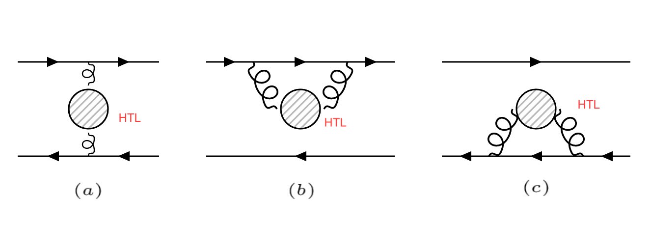
Fig. 1: The ”cross” diagram (a) corresponds to one $H_{I}$ from $U_{1}$ and one from $U_{2}$, and the two ”self-energy” diagrams (b) and (c) coming from quadratic expansions in $H_{I}$ in each $U_{1}$ and $U_{2}$ in (2.7).

The ”cross” diagram in Fig.1.(a) is the loss term, which relaxes the spin polarization of massive quarks, whereas the ”self-energy” diagram in Fig.1.(b) and (c) are the gain terms. The sum of all three diagrams preserves the total probability. Our result shows that the characteristic relaxation rate of spin polarization of massive quarks is of order $\alpha_{s}^{2}\log(1/\alpha_{s})$. The $\log$ contribution is coming from the t-channal soft gluon exchange with momentum scale from the Debye screening mass $m_{D}\sim gT$ to hard scale $T$.

3 Result and Summary

We obtain a separate time evolution equation for the particle number distribution and the spin polarization density in the leading log order of $g^{4}\log(1/g)$:

$${\partial f(\bm{p},t)\over\partial t}=C_{2}(F){m_{D}^{2}g^{2}\log(1/g)\over(4\pi)}\,{1\over 2pE_{p}}\,\Gamma_{f}\,,\quad{\partial\bm{S}(\bm{p},t)\over\partial t}=C_{2}(F){m_{D}^{2}g^{2}\log(1/g)\over(4\pi)}\,{1\over 2pE_{p}}\,\bm{\Gamma}_{S}\,,$$ (3.8)

where $\Gamma_{f}$ and $\bm{\Gamma}_{S}$ are diffusion-like differential operators in momentum space. They are given by:

$$\frac{\Gamma_{f}}{2pE_{p}} = \bm{\nabla}_{p^{i}}\Bigl{(}T(\frac{3}{4}-\frac{E_{p}^{2}}{4p^{2}}+\frac{\eta_{p}m^{4}}{4p^{3}E_{p}})\bm{\nabla}_{p^{i}}f(\bm{p})+\bm{p}^{i}\frac{Tm^{2}}{4p^{3}E_{p}}(\eta_{p}+\frac{3E_{p}}{p}-\frac{3\eta_{p}E_{p}^{2}}{p^{2}})\bm{p}\cdot\bm{\nabla}_{p}f(\bm{p})$$ (3.9)

$$+ \frac{\bm{p}^{i}}{2p^{2}}(E_{p}-\frac{\eta_{p}m^{2}}{p})f(\bm{p})\Bigr{)}$$

The above $\Gamma_{f}$ satisfies the nontrivial detailed balance condition, i.e. $\frac{\Gamma_{f}}{2pE_{p}}=0$ when $f(\bm{p})$ takes a form of the Boltzmann distribution function $f^{\rm eq}(\bm{p})=ze^{-E_{p}/T}$, where z is an arbitrary fugacity. It has been written as a total divergence so that the particle number is manifestly conserved. For $\bm{\Gamma}^{i}_{S}$, we have

$$\bm{\Gamma}^{i}_{S} = \left(2p+\frac{TE_{p}}{p}-\frac{\eta_{p}m^{2}T}{p^{2}}\right)\bm{S}^{i}(p)+\left(pTE_{p}-\frac{m^{2}TE_{p}}{2p}+\frac{\eta_{p}m^{4}T}{2p^{2}}\right)\bm{\nabla}_{p}^{2}\bm{S}^{i}(\bm{p})$$ (3.10)

$$+ \left(\frac{\eta_{p}m^{2}T}{2p^{2}}\left(1-\frac{3E^{2}_{p}}{p^{2}}\right)+\frac{3m^{2}TE_{p}}{2p^{3}}\right)(\bm{p}\cdot\bm{\nabla}_{p})^{2}\bm{S}^{i}(\bm{p})$$

$$+ \frac{1}{p^{2}}\left(pE^{2}_{p}-\frac{3m^{2}TE_{p}}{2p}+\eta_{p}m^{2}\left(-E_{p}-\frac{T}{2}+\frac{3TE^{2}_{p}}{2p^{2}}\right)\right)(\bm{p}\cdot\bm{\nabla}_{p})\bm{S}^{i}(\bm{p})$$

$$+ 2T\left(\eta_{p}\left(\frac{1}{2}-\frac{E^{2}_{p}}{p^{2}}+\frac{mE_{p}}{2p^{2}}+\frac{E^{3}_{p}}{2p^{2}(E_{p}+m)}\right)+\frac{E_{p}}{p}-\frac{m}{2p}-\frac{m^{2}}{2p(E_{p}+m)}\right)\left(\bm{p}^{i}(\bm{\nabla}_{p}\cdot\bm{S}(\bm{p}))-\bm{\nabla}_{p}^{i}(\bm{p}\cdot\bm{S}(\bm{p}))\right)$$

$$- \frac{T}{p^{2}}\left(\frac{E_{p}(E_{p}+2m)}{p(E_{p}+m)}+\frac{\eta_{p}mE_{p}}{E_{p}+m}\left(-\frac{3E_{p}}{p^{2}}+\frac{1}{E_{p}+m}\right)\right)\bm{p}^{i}({\bm{p}}\cdot\bm{S}(\bm{p}))\,.$$

Again one can check that $\frac{\bm{\Gamma}_{s}^{i}}{2pE_{p}}$ satisfies the nontrivial detailed balance condition in the massless limit when spin polarization density $\bm{S}(\bm{p})$ takes a form of $\bm{S}(\bm{p})=ze^{-\frac{p}{T}}\hat{\bm{p}}$.

We have derived the time evolution equation for the spin polarization of spin-$\frac{1}{2}$ massive quarks. It can be further improved in the future by going beyond the spatial homogeneity limit, i.e. by including the spatial gradients of the density matrix, and considering the vorticity and magnetic field effect.

I thank Ho-Ung Yee for fruitful collaborations. This material is based upon work supported by the U.S. Department of Energy, Office of Science, Office of Nuclear Physics, with the grant No. DE-SC0018209 and within the framework of the Beam Energy Scan Theory (BEST) Topical Collaboration.

References

- [1] L. Adamczyk et al. [STAR Collaboration],“Global hyperon polarization in nuclear collisions: evidence for the most vortical fluid,” Nature 548, 62 (2017)
- [2] Z. T. Liang and X. N. Wang, “Globally polarized quark-gluon plasma in non-central A+A collisions,” Phys. Rev. Lett. 94, 102301 (2005) Erratum: [Phys. Rev. Lett. 96, 039901 (2006)].
- [3] J. H. Gao, S. W. Chen, W. t. Deng, Z. T. Liang, Q. Wang and X. N. Wang, “Global quark polarization in non-central A+A collisions,” Phys. Rev. C 77, 044902 (2008).
- [4] F. Becattini, F. Piccinini and J. Rizzo, “Angular momentum conservation in heavy ion collisions at very high energy,” Phys. Rev. C 77, 024906 (2008).
- [5] M. Chiapparini, A. O. Gattone and B. K. Jennings, Nucl. Phys. A 529, 589 (1991).
- [6] N. Mueller and R. Venugopalan,“Constructing phase space distributions with internal symmetries,” Phys. Rev. D 99, no. 5, 056003 (2019)
- [7] N. Weickgenannt, X. L. Sheng, E. Speranza, Q. Wang and D. H. Rischke, “Kinetic theory for massive spin-1/2 particles from the Wigner-function formalism,” Phys. Rev. D 100, no. 5, 056018 (2019)
- [8] J. H. Gao and Z. T. Liang, “Relativistic Quantum Kinetic Theory for Massive Fermions and Spin Effects,” Phys. Rev. D 100, no. 5, 056021 (2019)
- [9] K. Hattori, Y. Hidaka and D. L. Yang, “Axial Kinetic Theory and Spin Transport for Fermions with Arbitrary Mass,” Phys. Rev. D 100 (2019) no.9, 096011
- [10] S. Li and H. U. Yee, “Quantum Kinetic Theory of Spin Polarization of Massive Quarks in Perturbative QCD: Leading Log,” Phys. Rev. D 100, no. 5, 056022 (2019)
- [11] J. I. Kapusta, E. Rrapaj and S. Rudaz, “Relaxation Time for Strange Quark Spin in Rotating Quark-Gluon Plasma,” Phys. Rev. C 101, no. 2, 024907 (2020)
- [12] D. L. Yang, K. Hattori and Y. Hidaka, “Quantum kinetic theory for spin transport: general formalism for collisional effects,” arXiv:2002.02612 [hep-ph].