Conformal geometry, Euler numbers, and global invertibility in higher dimensions

Abstract. It is shown that in dimension at least three a local diffeomorphism of Euclidean $n$-space into itself is injective provided that the pull-back of every plane is a Riemannian submanifold which is conformal to a plane. Using a similar technique one recovers the result that a polynomial local biholomorphism of complex $n$-space into itself is invertible if and only if the pull-back of every complex line is a connected rational curve. These results are special cases of our main theorem, whose proof uses geometry, complex analysis, elliptic partial differential equations, and topology.

AMS classification numbers: 14R15, 32H02, 53C21, 57R20

1 Introduction

The general question of deciding when a locally invertible map admits a smooth global inverse is a recurring theme in mathematics, about which much remains to be understood, even in the finite dimensional case. It encapsulates neatly, in the study of nonlinear systems with as many variables as equations, the questions of existence, uniqueness, and smooth dependence of the solution upon the value in the target space.

Given its wide scope, an all encompassing theory is not to be expected, but along the years many intriguing connections between global invertibility and different fields (e.g algebra, algebraic and differential geometry, complex analysis, non-linear analysis, topology, dynamical systems, and mathematical economics) have been unearthed. For a small sample of works dealing with this problem, where the search for new mechanisms of global invertibility is approached from a variety of points of view, we refer the reader to [1], [3] - [7], [9] - [17], [20] - [24], [26] - [28], [30], [31], [33] - [37], [39] - [47].

In this paper we concentrate on the issue of global injectivity. Our results, to be described shortly, also establish a new connection between topology and conformal geometry. From a technical standpoint, the main tool is the theory of linear elliptic partial differential equations.

As with many works on global invertibility, the theorems in this paper are of a “foundational” nature, being part of the overall effort of trying to understand the passage from local to global invertibility, in its many guises and for its own sake, without necessarily seeking to formulate invertibility criteria that can be readily implemented.

A historical example showing that this point of view is a fruitful one can be found in the pioneering works of J. Hadamard [27] in 1904 and of H. Cartan [7] in 1933. In modern language, the Hadamard invertibility theorem states that a local diffeomorphism $F:X\to Y$ between Banach spaces is bijective if $\sup_{x\in X}||DF(x)^{-1}||<\infty$ (see [40]). When $X=Y=\mathbb{R}^{n}$ this analytic condition can be replaced by the weaker requirement that all functionals $\langle F,v\rangle$, $v\neq 0$, satisfy the Palais-Smale condition [37].

The above condition in Hadamard’s theorem is rather strong, and this limits its use in applications. On the other hand, the underlying ideas are of great conceptual value, as they are behind the fundamental Cartan-Hadamard theorem in differential geometry - the statement that the exponential map of a complete manifold of non-positive sectional curvatures is a covering map -, which captures the essence, in a global sense, of non-positivity of curvature.

A topological result that subsumes the analytic result of [37] is the Balreira theorem [3], stating that a local diffeomorphism $F:\mathbb{R}^{n}\to\mathbb{R}^{n}$ is bijective if and only if the pre-image under $F$ of every affine hyperplane $H$ is non-empty and acyclic.

With the discovery of subtler manifestations of the global invertibility phenomenon - a slow but steady process -, increasingly more refined geometric and topological arguments have been invoked.

This can be seen in the circle of ideas that originated in [27] and [7], starting from simple covering spaces arguments (as in [40]), and leading to: degree theory and the Palais-Smale condition in [37]; foliations and intersection numbers in [3]; the Hopf fibration and the distortion theorems from the theory of univalent functions in [36]; dynamics and horocycles in geometries of negative curvature in [9], [16], [34] and [47]; conformal geometry, partial differential equations and the Poincaré-Hopf theorem in the present paper. Needless to say, other authors have also made contributions from a topological standpoint to the global invertibility program (see, for instance, [41], [42]).

The best known open problem in the area of global invertibility is, undoubtedly, the Jacobian conjecture ((JC), for short): Conjecture (JC). Every polynomial local biholomorphism $\mathbb{C}^{n}\to\mathbb{C}^{n}$ is invertible. Hundreds of papers have been written about (JC), mostly couched in algebraic arguments (general references are [5], [13]). On the other hand one should be cognizant of the fact that, despite casting a long shadow on the subject, (JC) is by no means the only outstanding problem in the study of global injectivity and related issues.

In order to dispel any misconception in this regard, and for the benefit of the reader, in section 11 we compile a list of roughly fifteen research problems, from different areas of mathematics, where the issue of global injectivity is at the forefront.

Returning to the description of the present work, we begin by refining the global injectivity question:

The singleton fiber problem. For an individual point $q$ in the image of a local diffeomorphism $F:M^{n}\to N^{n}$ between non-compact manifolds, under what extra conditions, involving only objects naturally associated to the point $q$ itself, can one conclude that the fiber $F^{-1}(q)$ consists of a single point?

In order to take into account the fact that the fibers of a local diffeomorphism $F$ may have different sizes, as $F$ need not be a cover map, (for instance, this happens in Pinchuk’s famous counterexample to the real Jacobian conjecture [39]), ideally any additional hypotheses required to guarantee $\#F^{-1}(q)=1$ should be sensitive to a possible change in the cardinality of nearby fibers, and thus they should involve only objects attached to $q$ itself. This is the rationale for including this condition in the above formulation of the singleton fiber problem. The results in this paper reflect this point of view.

In the next section the reader will find a short discussion of the so-called reduction theorems in the Jacobian conjecture ([5], [12], [28]), which will offer further motivation for the study of the singleton fiber problem.

Our aim in this work is to report on a new connection between conformal geometry, topology, elliptic partial differential equations, and the singleton fiber problem for a local diffeomorphism $F:N^{n}\to\mathbb{R}^{n}$, $n\geq 3$. In the process, we will extend and give a different perspective on some existing theorems on global invertibility.

To convey the flavor of our results, we state below a special case of an abstract geometric-topological criterion for a point to be covered only once (Theorem 8.1), that also yields necessary and sufficient conditions for invertibility in the Jacobian conjecture (see Theorem 8.2 as well as Theorem 9.1).

Theorem 1.1.

Let $F:\mathbb{R}^{n}\to\mathbb{R}^{n}$ be a local diffeomorphism, $n\geq 3$, and $q\in F(\mathbb{R}^{n})$. If the pre-image of every plane containing $q$ is a Riemannian submanifold of Euclidean space that is conformal to $\mathbb{R}^{2}$, a once punctured sphere, then $q$ is assumed exactly once by $F$. If, more generally, the pre-image of every such plane is conformal to a finitely punctured sphere, the number of punctures being allowed to vary with the plane, then $q$ is assumed at most twice by $F$.

Remark 1.2.

The hypothesis that $n$ should be at least $3$ is essential. In fact, every non-injective local diffeomorphism $\mathbb{R}^{2}\to\mathbb{R}^{2}$ constitutes a counterexample in two dimensions. We observe also that if $F:\mathbb{R}^{n}\to\mathbb{R}^{n}$ is a local diffeomorphism, $n\geq 3$, $q\in F(\mathbb{R}^{n})$, and the pre-image of every plane $\pi\ni q$ is homeomorphic to $\mathbb{R}^{2}\setminus D_{\pi}$ where $D_{\pi}$ is discrete, but $\#D_{\alpha}=\infty$ for at least one plane $\alpha\ni q$, then the fiber $F^{-1}(q)$ may actually be infinite [6].

The proof of Theorem 1.1 is based on a geometric construction involving the Poincaré-Hopf theorem on the relation between zeros of vector fields and the Euler characteristic, the classical Bôcher theorem on the structure of isolated singularities of positive harmonic functions in the plane, condenser-like Dirichlet problems on Riemann surfaces, and the general theory of linear elliptic differential equations.

The underlying ideas are rather conceptual, but the proof that certain sections of vector bundles are continuous require considerable work, as they involve using elliptic estimates on patches of manifolds, together with compactness arguments to extract convergent subsequences of subsequences, etc. These technical matters will be discussed in section $4$ and beyond.

Since the ideas in this work come from several areas (complex analysis, algebraic and differential geometry, topology and partial differential equations), we provide as much context and supply as many details as reasonably possible. In the same spirit, we hope that the broad list of problems compiled in section 11 can be useful to a reader interested in other aspects of global invertibility.

The author would like to express his heartfelt gratitude to his coauthor and now colleague, Scott Nollet, for countless enlightening conversations on the many facets of the theory of global invertibility. Thanks are also due to E. Cabral Balreira for explaining to us the Gale-Nikaido conjecture (see [17] and section 11 of the present paper), and to Luis Fernando Mello for his sustained interest in this work, as well as for explaining in detail the Pinchuk maps [34], [39].

This work is affectionately dedicated to my grandchildren, Lucca and Luna, ages 6 and 4. Hopefully they will enjoy the mildly anthropomorphic picture in section 7.

2 Vestigial forms of injectivity

In this section we discuss several examples to motivate the study of the problem of deciding when an individual fiber of a local diffeomorphism is a singleton, paving the way for the results to be proved in later sections.

In Example 1 we recall the reduction theorems from the algebraic study of the Jacobian conjecture (JC). This will be used to further motivate the study of the singleton fiber problem that was stated in the Introduction. In Example 2 we recall a result from [36], to the effect that a map as in (JC) is invertible if and only if the pre-images of complex lines are connected rational curves.

Examples 3 and 4 are a preamble for Theorem 1.1. In Example 5 we point out that any map as in (JC) is “coarsely injective”, in the sense that the pre-images of any real hyperplane is always connected (on the other end of the dimension spectrum, actual injectivity is equivalent to the condition that the pre-image of any point is connected). In Example 6 we discuss a simple conceptual application of differential geometry to the singleton fiber problem in the complex-analytic context.

2.1 Maps with unipotent Jacobians

Example 1.

Consider a polynomial map $F=I+H:\mathbb{R}^{n}\to\mathbb{R}^{n}$, $n\geq 2$ arbitrary, where $H$ is homogeneous of degree $3$ and $DH(x)$ is a nilpotent operator for every $x$. In particular, the only eigenvalue of $DF(x)=I+DH(x)$ is $1$, and so $F$ is a local diffeomorphism. Differentiating $H(tx)=t^{3}H(x)$ and setting $t=1$ one obtains the Euler relation $DH(x)x=3H(x)$, and from it the functional equation $DF(x)x=3F(x)-2x$. It follows from the latter that $0$ is covered exactly once by $F$, that is $F^{-1}(0)=\{0\}$. Indeed, if $x\neq 0$ and $F(x)=0$, one has $DF(x)x=-2x$, contradicting the fact that $\text{Spec}\;DF(x)=\{1\}$.

At first glance the above example seems contrived, but this is hardly the case. Rather than being special artifacts, these maps actually incorporate the general case of the above mentioned Jacobian conjecture (JC) in algebraic geometry, thanks to the so-called reduction theorems of Drużkowski [12] and Jagžev [28] (see also [5] and [13] for related developments).

The most basic version of the reduction theorems states that in order to prove (JC) it suffices to establish injectivity for all polynomial local biholomorphisms $G:\mathbb{C}^{n}\to\mathbb{C}^{n}$ of the form $G=I+K$, where $n$ is arbitrary, $K$ is homogeneous of degree $3$, and $DK(z)$ is nilpotent for every $z\in\mathbb{C}^{n}$. We shall refer to such a $G$ as a Drużkowski-Jagžev map. In fact, in [12] the map $K$ is further refined to be cubic linear.

Since the ground field is algebraically closed, nilpotency is actually a consequence of homogeneity and local invertibility. Conceivably, this (apparently new) observation can be used to simplify the proofs of the reduction theorems.

To see this, and arguing more generally, let $G=I+K:\mathbb{C}^{n}\to\mathbb{C}^{n}$ be a local biholomorphism, where $K$ is homogeneous of degree $k>1$. Assume the existence of $z_{0}\in\mathbb{C}^{n}$, $\lambda\in\mathbb{C}\setminus\{0\}$, and $v\in\mathbb{C}^{n}\setminus\{0\}$ such that $DK(z_{0})v=\lambda v$. If $\sigma\in\mathbb{C}$,

$$DG(\sigma z_{0})v=v+DK(\sigma z_{0})v=v+\sigma^{k-1}DK(z_{0})v=(1+\sigma^{k-1}\lambda)v.$$

Since $\lambda\neq 0$, one can choose $\sigma$ so that $1+\sigma^{k-1}\lambda=0$. Hence $DG(\sigma z_{0})v=0$, contradicting the fact that $G$ is everywhere a local biholomorphism. Hence, for every $z\in\mathbb{C}^{n}$, every eigenvalue $\lambda$ of $DK(z)$ must be zero. Thus, homogeneity of $K$ implies that $DK(z)$ is nilpotent, as claimed in the previous paragraph.

Let now $G:\mathbb{C}^{n}\to\mathbb{C}^{n}$ be an arbitrary holomorphic map, not necessarily polynomial, $z_{0}\in\mathbb{C}^{n}$ and $\widehat{G}:\mathbb{R}^{2n}\to\mathbb{R}^{2n}$ its realification, where $\mathbb{C}^{n}$ is identified with $\mathbb{R}^{2n}$ in the usual way. The Jacobian determinants of these maps are related by the well-known formula, a consequence of the Cauchy-Riemann equations:

$$\text{det}D\widehat{G}(z_{0})=|\text{det}DG(z_{0}|^{2}.$$ (2.1)

Applying (2.1) to $G-\lambda I_{\mathbb{C}^{n}}$, first with $\lambda\in\mathbb{R}$, one has

$$\text{det}(D\widehat{G}(z_{0})-\lambda I_{\mathbb{R}^{2n}})=\text{det}(D\widehat{G-\lambda I_{\mathbb{C}^{n}}})(z_{0})=|\text{det}(DG(z_{0})-\lambda I_{\mathbb{C}^{n}})|^{2}.$$

From

$$|\text{det}(DG(z_{0})-\lambda I_{\mathbb{C}^{n}})|^{2}=[\text{det}(DG(z_{0})-\lambda I_{\mathbb{C}^{n}})]\overline{[\text{det}(DG(z_{0})-\lambda I_{\mathbb{C}^{n}})]}$$

and

$$\overline{\text{det}(DG(z_{0})-\lambda I_{\mathbb{C}^{n}})}=\text{det}(\overline{DG(z_{0})}-\lambda I_{\mathbb{C}^{n}})$$

one has

$$\text{det}(D\widehat{G}(z_{0})-\lambda I_{\mathbb{R}^{2n}})=[\text{det}(DG(z_{0})-\lambda I_{\mathbb{C}^{n}})][\text{det}(\overline{DG(z_{0})}-\lambda I_{\mathbb{C}^{n}})],\;\;\lambda\in\mathbb{R}.$$ (2.2)

For $z_{0}$ fixed, (2.2) is an equality between polynomials in $\lambda\in\mathbb{R}$, and so the identity persists for $\lambda\in\mathbb{C}$ as well.

Observing that, for $\lambda\in\mathbb{C}$,

$$\text{det}(\overline{DG(z_{0})}-\lambda I_{\mathbb{C}^{n}})=\overline{[\text{det}(DG(z_{0})-\overline{\lambda}I_{\mathbb{C}^{n}})]},$$

one can rewrite the analogue of (2.2) for $\lambda\in\mathbb{C}$ as

$$\text{det}(D\widehat{G}(z_{0})-\lambda I_{\mathbb{R}^{2n}})=[\text{det}(DG(z_{0})-\lambda I_{\mathbb{C}^{n}})]\overline{[\text{det}(DG(z_{0})-\overline{\lambda}I_{\mathbb{C}^{n}})]},\;\;\lambda\in\mathbb{C}.$$ (2.3)

As an immediate consequence of (2.3), one has

$$\text{Spec}[D\widehat{G}(z_{0})]=\text{Spec}[DG(z_{0})]\cup\overline{\text{Spec}[DG(z_{0})]}.$$ (2.4)

If we now take $G=I+K$ to be a Drużkowski-Jagžev map in the discussion above, so that $DK(z)$ is nilpotent, it follows from (2.4) applied to $K$ that in $D\widehat{G}(z_{0})=I+D\widehat{K}(z_{0})$ the operator $D\widehat{K}(z_{0})$ is nilpotent as well.

In particular, the discussion in the first paragraph of this section, which was valid for real maps, applies when one takes $F=I+H=I+\widehat{K}:\mathbb{R}^{2n}\to\mathbb{R}^{2n}$. Consequently, $0$ is covered only once by $\widehat{G}$, the same being true of $G$ of course.

After one uses the fact that a polynomial local biholomorphism is a cover map away from a certain algebraic hypersurface, one has the following (known) invertibility criterion in (JC):

$\bf(\dagger)\rm$ (JC) holds if and only if one can show, for any given Drużkowski-Jagžev map $G=I+K:\mathbb{C}^{n}\to\mathbb{C}^{n}$, that there exists some neighborhood $U$ of $0$ in $\mathbb{R}^{2n}$ for which $\underline{every}$ $q\in U$ is covered exactly once by the induced $\underline{real}$ map $\widehat{G}=I+\widehat{K}:\mathbb{R}^{2n}\to\mathbb{R}^{2n}$.

The simple-minded argument using Euler’s relation from the beginning of this section shows that $q=0$ is covered only once by $\widehat{G}$, but says nothing of the sort if $q\approx 0$.

In the context of the Jacobian conjecture injectivity implies surjectivity, and so $\bf(\dagger)\rm$ lends extra support to the need to investigate, even in the general case of local diffeomorphisms - as opposed to just local biholomorphisms -, the sensitive question of how the cardinality varies when one considers nearby fibers. This is, in essence, the idea behind the singleton fiber problem.

2.2 The gradation $(\diamondsuit_{d})_{d=0}^{n-1}$ for coarse injectivity

In order to provide context for the theorems in this paper, let us first consider the injectivity question from a naïve topological standpoint.

It is nearly tautological that a point $q$ in the image of a local diffeomorphism $F:N^{n}\to\mathbb{R}^{n}$ is covered only once if (and only if) $F^{-1}(q)$ is connected. One is then led to the following question, where $d$ is a non-negative integer, $0\leq d\leq n-1$: Definition/Question (Coarse injectivity). If the pre-image under a local diffeomorphism $F:N^{n}\to\mathbb{R}^{n}$ of all $d$-dimensional affine subspaces through $q$ are connected, then one says that $(F,q)$ satisfies property $(\bf\diamondsuit_{d})$. As observed above, property $(\bf\diamondsuit_{0})$ is equivalent to $\#F^{-1}(q)=1$. If $d>0$, does $(\bf\diamondsuit_{d})$ imply $\#F^{-1}(q)=1$? This question will be taken up in the next subsections. The answers that we will obtain along the way will lead us to the new theorems proven in this paper.

Example 2.

The main impetus for exploring the idea of injectivity as a connectedness phenomenon stems from the Jacobian Conjecture, since there are powerful results in the literature about the connectedness of algebraic varieties (Bertini theorems). An example in the algebraic setting of the link between connectedness and injectivity, albeit not directly motivated by $(\bf\diamondsuit_{d})$, is the following injectivity criterion in the Jacobian conjecture, first established in [36] as a consequence of a more general theorem (see also Theorem 8.2 in the present paper for a new proof): $\bf(\dagger\dagger)\rm$A polynomial local biholomorphism $F:\mathbb{C}^{n}\to\mathbb{C}^{n}$, $n>1$, is invertible if and only if for the general point $q$ in $F(\mathbb{C}^{n})$, the pre-image under $F$ of every complex line containing $q$ is homeomorphic to an open domain of $\mathbb{R}^{2}$ (i.e. the pre-image is a connected rational curve, in the language of algebraic geometry). More generally, the main result in [36] asserts the injectivity of any local biholomorphism $V^{n}\to\mathbb{C}^{n}$, $n>1$, for which the pre-images of all complex lines are biholomorphic to $\mathbb{C}\mathbb{P}^{1}$ punctured finitely many times, the number of punctures being allowed to vary with the complex line.

2.3 $(\diamondsuit_{1})$ $\Longrightarrow(\diamondsuit_{0})$

Example 3.

As observed before, $(\bf\diamondsuit_{0})$ is equivalent to $q$ being covered only once. Elementary arguments show that $(\diamondsuit_{1})$ $\Longrightarrow(\diamondsuit_{0})$ in the following form: $\#F^{-1}(q)=1$ provided that $\underline{\rm some}$ $\underline{\rm line}$ through $q$ has a connected pre-image. To see this, let $l$ be a line containing $q$ for which $F^{-1}(l)$ is connected. By the classification theorem for connected $1$-manifolds, $F^{-1}(l)$ is diffeomorphic either to $\mathbb{R}$ or to a circle $S^{1}$. The restriction map $F^{-1}(l)\stackrel{{\scriptstyle F}}{{\to}}l$ is a local diffeomorphism, so its image is an open set. If $F^{-1}(l)\approx S^{1}$, the image of the restriction map would be compact (hence closed) and also open. By connectedness, the image would be the entire line $l$ and yet compact, a contradiction. It follows that $F^{-1}(l)\approx\mathbb{R}$. Since a local diffeomorphism of $\mathbb{R}$ into itself is strictly monotonic, hence injective, $F^{-1}(l)\stackrel{{\scriptstyle F}}{{\to}}l$ must also be injective, and therefore $q$ is covered exactly once by $F$. This establishes $(\bf\diamondsuit_{1})$ .

Dynamically, $(\bf\diamondsuit_{1})$ can be understood as follows. Consider the two rays in $l$ with initial point $q$, and assume $a,b\in F^{-1}(l)$ are distinct points mapped into $q$. Start lifting through $a$ the ray in $l$ that corresponds to moving along $F^{-1}(l)$ in the direction of $b$. If the ray cannot be lifted in its entirety then the lift rushed to infinity in finite time, in which case it passes through $b$. Evidently, the lift also contains $b$ if the ray can be lifted in its entirety. Hence, regardless, the maximal lift through $a$ of the appropriate ray starting at $q$ must contain $b$. Looking at the images, since $F(a)=F(b)=q$, this means that at first the image of the lift moved away from $q$, along the line $l$, but then it “switched directions” and came back to $q$. Hence, the differential of $F$ must have become singular somewhere in $F^{-1}(l)$, contradicting the fact that $F$ is everywhere a local diffeomorphism.

As the previous argument relies on monotonicity, one might expect the answer to whether $(\bf\diamondsuit_{2})$ implies $(\bf\diamondsuit_{0})$ to be negative. This is indeed the case, as shown by the example below.

2.4 Generic unknots and $(\diamondsuit_{2})$

Example 4.

We exhibit a local diffeomorphism $F:N^{3}\to\mathbb{R}^{3}$ for which the fiber of some $q\in F(N^{3})$ has infinitely many points, and yet the pre-image of every plane passing through $q$ is a connected surface.

Start with the specific unknot $\Gamma\subset\mathbb{R}^{3}$ depicted in Fig.1. Positioning $\Gamma$ appropriately, vis-à-vis the origin $0$, the following conditions hold for any two-dimensional vector subspace $V\subset\mathbb{R}^{3}$: $0\notin\Gamma$, $V\cap\Gamma$ is non-empty, finite, and there is at least one point in $\Gamma\cap V$ where the intersection is transversal.

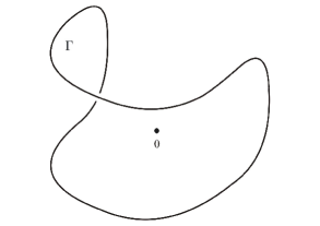
Fig. 1: For every plane $V$ through $0\notin\Gamma$, $V\pitchfork_{p}\Gamma$ for at least one $p$ in the finite set $V\cap\Gamma$.

Let $F:N\to\mathbb{R}^{3}-\Gamma\subset\mathbb{R}^{3}$ be the universal cover map. As $\pi_{1}(\mathbb{R}^{3}-\Gamma,0)=\mathbb{Z}$, $F^{-1}(0)$ is infinite. The reader is asked to visualize that, given any two-dimensional vector subspace $V$ of $\mathbb{R}^{3}$, $A_{V}\stackrel{{\scriptstyle def}}{{=}}V-(V\cap\Gamma)$ is connected. Also, a “thin” loop in $A_{V}$ that is based at $0$ and encircles only once some point where the intersection $V\cap\Gamma$ is transversal represents a generator of $\pi_{1}(\mathbb{R}^{3}-\Gamma,0)$. It follows that the inclusion $i:A_{V}\to\mathbb{R}^{3}-\Gamma$ induces an epimorphism $i_{*}:\pi_{1}(A_{V},0)\to\pi_{1}(\mathbb{R}^{3}-\Gamma,0)$, and so $F^{-1}(V)=F^{-1}(A_{V})$ is connected [32, p.179]. Hence $(\bf\diamondsuit_{2})$ does not imply $(\bf\diamondsuit_{0})$ (see also [6] and problem xiv), section 11).

In section 4 we introduce a condition stronger than the topological condition $(\bf\diamondsuit_{2})$, of a conformal nature, whose validity implies that $F^{-1}(q)$ is a singleton.

2.5 $(\diamondsuit_{\text{2n-1}})$ holds in (JC)

Example 5.

Since $(\bf\diamondsuit_{0})$ and $(\bf\diamondsuit_{1})$ both lead to the fiber being a singleton, but $(\bf\diamondsuit_{2})$ does not, one can think of the property that the pre-images of all $d$-dimensional affine subspaces are connected, for some $d$ in the range $2\leq d\leq n-1$, as a coarse form of injectivity.

It is amusing that this vestigial form of injectivity always holds in the Jacobian conjecture setting, for the top value $d=2n-1$. Of course, (JC) claims that $(\bf\diamondsuit_{d})$ already holds at the level $d=0$.

Theorem 2.1.

If $\widehat{F}:\mathbb{R}^{2n}\to\mathbb{R}^{2n}$ is the realification of a polynomial local biholomorphism $F:\mathbb{C}^{n}\to\mathbb{C}^{n}$, then $(\widehat{F})^{-1}(H^{2n-1})$ is connected for every real hyperplane $H^{2n-1}\subset\mathbb{R}^{2n}$.

This is a previously unpublished result by S. Nollet and F. Xavier. Below, we provide the arguments when $n=2$.

Write $z_{1},z_{2}$ for the coordinates in the domain of $F=(F_{1},F_{2}):\mathbb{C}^{2}\to\mathbb{C}^{2}$, and $w_{1}=u_{1}+iv_{1}$, $w_{2}=u_{2}+iv_{2}$ for the coordinates in the co-domain. The natural identification between $\mathbb{C}^{2}$ and $\mathbb{R}^{4}$ is $(w_{1},w_{2})\to(u_{1},v_{1},u_{2},v_{2})$. We are supposed to show that $F^{-1}(H^{3})$ is connected for every real hyperplane $H^{3}$. Choosing coordinates appropriately, it suffices to take $H^{3}$ to be the hyperplane $u_{1}=0$.

Consider the projection $\Lambda:H^{3}\to\mathbb{R}$, $\Lambda(0,t,v_{1},v_{2})=t$. Under the identification, $H^{3}$ is foliated by the complex lines $V_{t}=\{(w_{1},w_{2})\;|\;w_{1}=it\}$, $t\in\mathbb{R}$. Observe that $F^{-1}(V_{t})=(F_{1})^{-1}(it)$ is non-empty for every $t$ because the polynomial $F_{1}:\mathbb{C}^{n}\to\mathbb{C}$ is non-constant, hence surjective by the fundamental theorem of algebra.

A complex polynomial $p(z_{1},z_{2})$ is said to be primitive if the fibers $\{p=c\}\subset\mathbb{C}^{2}$ are connected, with the possible exception of finitely many values of $c$. It is a classical result that if $p$ is $\underline{\rm not}$ primitive then it can be decomposed as $p=q\circ r$, where $q:\mathbb{C}\to\mathbb{C}$ is a polynomial of degree at least two, and $r$ is a polynomial in two variables. We claim that if $p$ has no critical points, then $p$ is primitive.

In order to see this, we argue by contradiction. In the decomposition $p=q\circ r$ the polynomial $r$ is necessarily non-constant, and so it assumes all complex numbers. The gradients satisfy $\nabla p(z)=q^{\prime}(r(z))\nabla r(z)$. If $z$ is chosen so that $r(z)$ is a zero of $q^{\prime}$ (which is possible because $\text{deg}\;q^{\prime}\geq 1$), then $\nabla p(z)=0$, a contradiction. This establishes our claim.

Observe that the polynomial $F_{1}$ has no critical points (otherwise $\text{det}DF$ would vanish somewhere) and therefore, by the previous paragraph, $F_{1}$ is primitive. In particular, there areat most finitely many values of $t\in\mathbb{R}$, say $t_{1},\dots,t_{k}$, for which the (necessarily non-empty) set $F^{-1}(V_{t_{j}})=(F_{1})^{-1}(it_{j})$ is disconnected.

We can now show that $F^{-1}(H^{3})$ is connected. Again arguing by contradiction, write

$$F^{-1}(H^{3})=\displaystyle\bigcup_{t\in\mathbb{R}}F^{-1}(V_{t})=U_{1}\cup U_{2},$$

where $U_{1}$, $U_{2}$ are non-empty, open, and disjoint. Set $J_{k}=\{t\in\mathbb{R}:F^{-1}(V_{t})\cap U_{k}\neq\emptyset\}.$ As remarked before, $F^{-1}(V_{t})\neq\emptyset$ for every $t\in\mathbb{R}$, so that $J_{1}\cup J_{2}=\mathbb{R}$. Since $F$ is locally invertible, each $J_{k}$ is a non-empty open set. From the connectedness of $\mathbb{R}$, $J_{1}\cap J_{2}$ is a non-empty open set. In particular, we can select $\overline{t}\in J_{1}\cap J_{2}\setminus\{t_{1},\dots,t_{k}\}$. It is now clear that $F^{-1}(V_{\overline{t}})\cap U_{1}$ and $F^{-1}(V_{\overline{t}})\cap U_{2}$ form a disconnection of $F^{-1}(V_{\overline{t}})$, a contradiction. This shows that $F^{-1}(H^{3})$ is connected, concluding the proof of Theorem 2.1.

3 A differential-geometric mechanism for injectivity

Example 6.

The following example from [36] is a conceptual application of topology and differential geometry to the singleton fiber problem, in the context of complex analysis. It is based on the fact that the Hopf map does not admit continuous sections.

($\bullet$) Let $F:\mathbb{C}^{n}\to\mathbb{C}^{n}$, $n\geq 2$, be a local biholomorphism and $q$ a point in the image of $F$. If the pre-image of every complex line $l$ containing $q$ is connected and simply-connected, then $q$ is assumed exactly once by $F$.

To see this, assume that $F(a)=F(b)=q$, $a\neq b$. We may assume $q=0$. By hypothesis, the complex curve $F^{-1}(l)$ contains $a$ and $b$ for every such $l$. Since $F^{-1}(l)$ is properly embedded (because $F$ is a local bihilomorphism), it follows that $F^{-1}(l)$ is a complete, connected, simply-connected Riemannian surface of non-positive curvature.

By the Cartan-Hadamard theorem alluded to in the Introduction, there is a unique geodesic in $F^{-1}(l)$ that connects $a$ to $b$. Let $v_{l}$ be the unit tangent vector at $a$ of this geodesic. The set of complex lines passing through $q$ is naturally identified with $\mathbb{C}\mathbb{P}^{n-1}$. We can then define a map

$$s:\mathbb{C}\mathbb{P}^{n-1}\to S^{2n-1},\;\;s(l)=\frac{DF(a)v_{l}}{|DF(a)v_{l}|}\in l\cap S^{2n-1}.$$ (3.1)

Consider the Hopf map $\pi:S^{2n-1}\to\mathbb{C}\mathbb{P}^{n-1}$ that associates to a point in the unit sphere the unique complex line passing through it and the origin. It follows from (3.1) that $s$ is a section of $\pi$. Since one can argue that $s$ is continuous, invoking the continuous dependence of solutions of systems of ordinary differential equations upon the initial conditions as well as parameters, we arrive at a contradiction.

A considerable elaboration of the above arguments leads to a sharp estimate on the cardinality of the fibers of certain local biholomorphisms. The theorem below is a special case of the main result of [9]:

Theorem 3.1.

Let $F:\mathbb{C}^{2}\to\mathbb{C}^{2}$ be a local biholomorphism, $d$ a positive integer, $q$ a point in the image of $F$, and $\mathcal{L}$ the set of all complex lines passing through $q$. Assume that : i) For every $l\in\mathcal{L}$ the complex curve $F^{-1}(l)$ has at most $d$ connected components. ii) There exists a finite set $\mathcal{F}\subset\mathcal{L}$ such that $F^{-1}(l)$ is $1$-connected for all $l\in\mathcal{L}-\mathcal{F}$. Then the fiber $F^{-1}(q)$ has at most $d$ points.

That the theorem is sharp can be seen by taking $q=0$ and $F(z,w)=(f(z),w)$, where $f:\mathbb{C}\to\mathbb{C}$ is holomorphic, $f^{\prime}$ is nowhere zero, and $\#f^{-1}(0)=d$ (see [9] for details).

4 A topological-conformal enhancement of $(\bf\diamondsuit_{2})$

Notwithstanding Example 4, it is possible to strengthen $(\bf\diamondsuit_{2})$ so that the enhanced property implies $\#F^{-1}(q)=1$. Loosely speaking, one needs to go beyond mere connectedness by requiring that the pre-images of all planes containing the point $q$ be diffeomorphic to $\mathbb{R}^{2}$ and also “conformally large”.

It is a classical result that every orientable Riemannian surface $(M,g)$ can be given a Riemann surface structure, where local holomorphic coordinates $z=x+iy$ can be introduced so that, relative to these so-called isothermal parameters the metric $g$ is locally conformally flat, meaning that it assumes the form $g(x,y)=\lambda^{2}(x,y)(dx^{2}+dy^{2})$ for some smooth function $\lambda>0$ ([8], [18, p. 19], [29, Thm. 3.11.1]).

Unless otherwise stated, we shall agree that in this paper the conformal (or complex) structure associated to any orientable surface $M$ embedded in some euclidean space $\mathbb{R}^{k}$ will be the one arising from the Riemannian metric on $M$ obtained by the restriction of the standard inner product of $\mathbb{R}^{k}$. We write $q+\pi$ for the plane containing the point $q$ that is parallel to the two-dimensional vector subspace $\pi$ of $\mathbb{R}^{n}$. As usual, $G_{2}(\mathbb{R}^{n})$ stands for the Grassmannian of two-dimensional vector subspaces of $\mathbb{R}^{n}$. The following result is stated first in the language of differential geometry.

Theorem 4.1.

Let $F:\mathbb{R}^{n}\to\mathbb{R}^{n}$ be a local diffeomorphism, $n\geq 3$, $q\in F(\mathbb{R}^{n})$. Assume the existence of a compact orientable surface $M^{2}$ embedded in $\mathbb{R}^{n}$ such that $\chi(M^{2})\neq 0$ and, for every $\pi\in G_{2}(\mathbb{R}^{n})$ that is parallel to some tangent plane of $M^{2}$, the surface $F^{-1}(q+\pi)\subset\mathbb{R}^{n}$ is conformally diffeomorphic to $\mathbb{R}^{2}$. Then the fiber $F^{-1}(q)$ consists of a single point.

In complex-analytic terms, the hypothesis of Theorem 4.1 stipulates that the (necessarily non-compact) one-dimensional complex manifold $F^{-1}(q+\pi)$ is connected, simply-connected, and biholomorphic to $\mathbb{C}$ rather than to an open disc $D$ (by the Koebe uniformization theorem, a $1$-connected Riemann surface is biholomorphic to $\mathbb{C}\mathbb{P}^{1}$, $\mathbb{C}$, or $D$).

The next result yields information about the cardinality of the fiber $F^{-1}(q)$ when $F^{-1}(q+\pi)$ is allowed to be conformal to a sphere $S^{2}$ punctured finitely many times (and not just once, as in Theorem 4.1):

Theorem 4.2.

Let $F:\mathbb{R}^{n}\to\mathbb{R}^{n}$ be a local diffeomorphism, $n\geq 3$, $q\in F(\mathbb{R}^{n})$. Assume the existence of a compact orientable surface $M^{2}$ embedded in $\mathbb{R}^{n}$ such that $\chi(M^{2})\neq 0$ and, for every $\pi\in G_{2}(\mathbb{R}^{n})$ that is parallel to some tangent plane of $M^{2}$, there exist points $p_{1},\dots,p_{k_{\pi}}\in S^{2}$, $k_{\pi}\geq 1$, for which the surface $F^{-1}(q+\pi)\subset\mathbb{R}^{n}$ is conformally diffeomorphic to $S^{2}-\{p_{1},\dots,p_{k_{\pi}}\}$. Then the fiber $F^{-1}(q)$ has at most two points.

Taking $M^{2}$ to be a compact orientable surface in $\mathbb{R}^{n}$ other than a torus in Theorems 4.1 and 4.2, one has:

Corollary 4.3.

Let $F:\mathbb{R}^{n}\to\mathbb{R}^{n}$ be a local diffeomorphism, $n\geq 3$. If the pre-image under $F$ of every affine plane is a surface conformal to $\mathbb{R}^{2}$, then $F$ is injective.

Corollary 4.4.

Let $F:\mathbb{R}^{n}\to\mathbb{R}^{n}$ be a local diffeomorphism, $n\geq 3$. If the pre-image under $F$ of every affine plane is a surface conformal to a finitely punctured sphere, the number of punctures being allowed to vary with the plane, then every point in $\mathbb{R}^{n}$ is covered at most twice by $F$.

The two-dimensional analogue of Corollary 4.3 fails dramatically. Indeed, $\underline{\rm every}$ non-injective local diffeomorphism $F:\mathbb{R}^{2}\to\mathbb{R}^{2}$ provides a counterexample. Examples include the realification of the complex exponential and the Pinchuk counterexamples to the so-called real Jacobian conjecture [39].

A reasonable conjecture seems to be that the estimate $\#F^{-1}(q)\leq 2$ in Theorem 4.2 can be improved to $\#F^{-1}(q)=1$, a result that would of course be stronger than the conclusion in Theorem 4.1.

The proof of Theorem 4.1 is fairly long and technical, but we can highlight here some of the main points. The central idea is that if the fiber $F^{-1}(q)$ had at least two distinct elements, then one could construct a continuous nowhere zero vector field on $M^{2}$, thus contradicting the Poincaré-Hopf theorem since $\chi(M^{2})\neq 0$.

The construction of this vector field explores the special nature of the isolated singularities of positive harmonic functions in the plane. To establish continuity – the more involved part of the proof –, one uses Bôcher’s theorem and the standard theory of linear elliptic partial differential equations, after some technical difficulties have been overcome.

In Section 7 we give a fairly conceptual proof of Theorem 4.2. It uses the solutions of certain Dirichlet problems on the Riemann surfaces $F^{-1}(q+\pi)$, in a manner reminiscent of the notion of condensers in classical potential theory, in order to create, under the assumption that the fiber has at least three elements, a continuous non-vanishing vector field on $M^{2}$. This contradiction shows that the fiber has at most two elements.

These results are actually special cases of a general abstract mechanism for global injectivity, codified in Theorem 8.1, that may yet be useful in other settings. With the aid of the algebro-geometric result that the generic fiber of a polynomial local biholomorphism $F:\mathbb{C}^{n}\to\mathbb{C}^{n}$ cannot have cardinality two, Theorem 8.1 yields another proof of the necessary and sufficient condition for invertibility in (JC) that was first established in [36] (see Example 2 in section 2 and Theorem 8.2).

Theorem 9.1 is a new result, a necessary and sufficient condition for invertibility in the Jacobian conjecture when the polynomial map has $\underline{\rm real}$ coefficients. It stands as a natural companion to Theorem 8.2. Besides the condenser construction from section 7, the proof of Theorem 9.1 uses “symmetry” arguments and the fact that the Euler number of the tautological line bundle is non-zero mod (2).

5 Using Bôcher’s theorem to create vector fields

In this section we begin the proof of Theorem 4.1, which is couched on two closely related classical results about isolated singularities of positive harmonic functions.

Lemma 5.1 will be used in this section in the course of a geometric construction aimed at establishing the existence of certain vector fields on $M^{2}$. Lemma 5.2 - actually a theorem of Bôcher -, will play a central role in the continuity proof of the said vector field. This is a lengthy argument, presented in section 6, that also uses the general theory of linear elliptic equations.

In what follows, we set $B=\{z\in\mathbb{C}:|z|<1\}$.

Lemma 5.1.

([2], p. 52) Let $u$ be positive and harmonic on $B\setminus\{0\}$, $u(z)\to 0$ as $|z|\to 1$. Then there exists a constant $c>0$ such that $u(z)=-c\log|z|$, $z\in B\setminus\{0\}$.

Lemma 5.2.

([2], p. 50) Let $u$ be positive and harmonic on $B\setminus\{0\}$. Then there is a harmonic function $\nu$ on $B$ and a constant $c\geq 0$, with $u(z)=\nu(z)-c\log|z|,z\in B\setminus\{0\}.$

Let $F$ be as in the statement of Theorem 4.1. Replacing $F$ by $F-q$ we may, and will, assume that $q=0$. Suppose, by contradiction, that $F^{-1}(0)$ contains at least two distinct points, say $a$ and $b$. Consider an open neighborhood $U$ of $a$ and an Euclidean ball $W$ centered at $0$ such that $b\notin\overline{U}$ and $U\xrightarrow[]{F}W$ is a diffeomorphism.

Let $\pi\subset\mathbb{R}^{n}$ be a plane containing $q=0$ that is parallel to some tangent plane of $M^{2}$. We shall denote by $\mathcal{A}$ the totality of such $\pi$, so that $\mathcal{A}$ may be regarded as a subset of the Grassmannian $G_{2}(\mathbb{R}^{n})$ of two-dimensional vector subspaces of $\mathbb{R}^{n}$. Observe that $a,b\in F^{-1}(\pi)$ for all $\pi\in\mathcal{A}$. We will abuse the notation somewhat and write interchangeably $\pi\in G_{2}(\mathbb{R}^{n})$ or $\pi\subset\mathbb{R}^{n}$. Set

$$U_{\pi}=U\cap F^{-1}(\pi),\;\;T_{\pi}=\partial(U\cap F^{-1}(\pi)).$$ (5.1)

Denote by $\Delta_{\pi}$ the Riemannian Laplacian on the simply-connected surface $F^{-1}(\pi)$, associated to the metric $g_{\pi}$ on $F^{-1}(\pi)$ obtained by the restriction of the Euclidean metric $g$ of $\mathbb{R}^{n}$.

In local conformal coordinates $z=x+iy$ on $F^{-1}(\pi)$, $g_{\pi}$ and $\Delta_{\pi}$ are given by

$$g_{\pi}=\lambda^{2}|dz|^{2},\;\;\Delta_{\pi}=4\lambda^{-2}\partial_{z}\partial_{\overline{z}},$$

where $\lambda$ is a positive smooth function, and

$$\partial_{z}=\frac{1}{2}(\partial_{x}-i\partial_{y}),\;\;\;\partial_{\overline{z}}=\frac{1}{2}(\partial_{x}+i\partial_{y}).$$

Hence, a function on $F^{-1}(\pi)$ is $\Delta_{\pi}$-harmonic (i.e. harmonic in the sense of the Riemannian metric $g_{\pi}$) if and only if it is harmonic in the sense of the Riemann surface structure of $F^{-1}(\pi)$ induced by the isothermal parameters $z$ above.

Lemma 5.3.

For each $\pi$ as before there exists a unique function $u_{\pi}:F^{-1}(\pi)\setminus\overline{U}_{\pi}\to[0,\infty)$ satisfying the following properties: i) $u_{\pi}$ is $\Delta_{\pi}$-harmonic. ii) $\lim u_{\pi}(p)=\infty$ uniformly as $|p|\to\infty$ in $\mathbb{R}^{n}$, $p\in F^{-1}(\pi)\setminus\overline{U_{\pi}}$. iii) $\lim u_{\pi}(p)=0$ as $p\to T_{\pi}$, $p\in F^{-1}(\pi)\setminus\overline{U_{\pi}}$. iv) $u_{\pi}(b)=1$. Furthermore, $du_{\pi}(b)\neq 0$.

The proof of Lemma 5.3 proceeds as follows. Recall that we are working under the assumption that, for all $\pi\in\mathcal{A}$, the Riemann surface $F^{-1}(\pi)$ is conformal to the complex plane $\mathbb{C}$. Hence $F^{-1}(\pi)\setminus\overline{U}$ is conformal to a punctured neighborhood of infinity in the Riemann sphere which, in turn, is conformal to $B\setminus\{0\}$.

As the biholomorphic self-maps of $B\setminus\{0\}$ are rotations about $0$, it follows that there is a unique conformal map $h_{\pi}:F^{-1}(\pi)\setminus\overline{U_{\pi}}\to B\setminus\{0\}$ such that $h_{\pi}(b)\in(0,\infty)\cap B$.

Consider the function $v_{\pi}:B\setminus\{0\}\to(0,\infty)$,

$$v_{\pi}(z)=\frac{\log|z|}{\log(h_{\pi}(b))},\;\;z\in B\setminus\{0\}.$$ (5.2)

Observe that

$$|\lim_{p\to T}h_{\pi}(p)|=1,\;\;\;\lim_{||p||\to\infty}h_{\pi}(p)=\infty$$ (5.3)

It is now clear that $u_{\pi}\stackrel{{\scriptstyle def}}{{=}}v_{\pi}\circ h_{\pi}$ satisfies properties i)-iv) above, settling the existence part of Lemma 5.3. Furthermore, $du_{\pi}(b)\neq 0$ because $v_{\pi}$ has no critical points.

In order to establish uniqueness, assume that $\tilde{u}_{\pi}$ is non-negative and satisfies i)-iv). It follows from (5.3) and iii) that $\tilde{v}_{\pi}:=\tilde{u}_{\pi}\circ(h_{\pi})^{-1}:B\setminus\{0\}\to(0,\infty)$ satisfies the hypothesis of Lemma 5.1, and so $\tilde{v}_{\pi}(z)=-c\log|z|$ for some $c>0$ and all $z\in B\setminus\{0\}$. From (iv),

$$1=\tilde{u}_{\pi}(b)=\tilde{v}_{\pi}(h_{\pi}(b))=-c\log|h_{\pi}(b)|.$$

Solving for $-c$ and using (5.2) one has $v_{\pi}=\tilde{v}_{\pi}$, and so $u_{\pi}=\tilde{u}_{\pi}$. This concludes the proof of Lemma 5.3.

∎Continuing with the proof of Theorem 4.1, for $p\in M^{2}$ let $\pi_{p}=T_{p}M^{2}$ be the tangent space of $M$ at $p$ (hence a two-dimensional vector space, naturally identified with an element of $G_{2}(\mathbb{R}^{n})$).

Recall that the Riemannian gradient $\nabla u_{\pi_{p}}(b)$, where $u_{\pi_{p}}$ is given by Lemma 5.3, is the vector in the tangent space $T_{b}(F^{-1}(\pi_{p}))$ that represents, in the inner product sense, the differential $du_{\pi_{p}}(b):T_{b}(F^{-1}(\pi_{p}))\to\mathbb{R}$.

Lemma 5.4.

The map $s:M^{2}\to\mathbb{R}^{n}$ given by

$$s(p)=dF(b)\nabla u_{\pi_{p}}(b),\,\;p\in M^{2},$$ (5.4)

defines a non-vanishing vector field on $M^{2}$.

Indeed, for all $p\in M^{2}$ one has $\nabla u_{\pi_{p}}(b)\in T_{b}(F^{-1}(T_{p}M^{2}))$, and since $b\in F^{-1}(T_{p}M^{2})$, on account of $F(b)=q=0$, one has

$$s(p)=dF(b)\nabla u_{(T_{p}M^{2})}(b)\in dF(b)[T_{b}(F^{-1}(T_{p}M^{2}))]=T_{F(b)}T_{p}M^{2}=T_{0}T_{p}M^{2}\approx T_{p}M^{2},$$

so that $s$ is a section of the tangent bundle $TM^{2}$, i.e a vector field on $M^{2}$. Since $\nabla u_{(T_{p}M^{2})}(b)\neq 0$ by Lemma 5.3, and $dF(b)$ is non-singular ($F$ is a local diffeomorphism), it follows from (5) that $s(p)\neq 0$ for all $p\in M^{2}$.

∎

Proof of Theorem 4.1.

It will be shown in the next section, using a lengthy argument, that the nowhere zero vector field on $M^{2}$ defined in Lemma 5.4, and whose construction depends in an essential way on the assumption $\#F^{-1}(q)=\#F^{-1}(0)\geq 2$, is continuous. But this contradicts the Poincaré-Hopf theorem [38] because $\chi(M^{2})\neq 0$, and so $F^{-1}(0)$ must be a singleton, thus completing the proof of Theorem 4.1.

6 Elliptic estimates and the continuity argument

Our goal in this section is to finish the proof of Theorem 4.1 by showing that the vector field $s$ given in Lemma 5.4 is continuous. The proof uses the general theory of linear elliptic partial differential equations, as well as the Bôcher theorem (Lemma 5.2).

Recall from the previous section that we are working under the assumption that $F(a)=F(b)=0$, $a\neq b$. To keep the notation at a manageable level, we continue setting $\pi_{p}=T_{p}M^{2}$. The vector field $s$ from Lemma 5.4 is given by

$$s(p)=dF(b)\nabla u_{\pi_{p}}(b)\in T_{F(b)}T_{p}M^{2}=T_{0}T_{p}M^{2}\cong T_{p}M^{2},\;p\in M^{2}.$$ (6.1)

In order to establish the continuity of $s$ at $z\in M^{2}$, it suffices to show that for every sequence $(z_{k})$ in $M^{2}$ that converges to $z$ there is a subsequence $z_{k_{j}}$ such that

$$s(z_{k_{j}})=dF(b)\nabla u_{\pi_{z_{j}}}(b)\to dF(b)\nabla u_{\pi_{z}}(b)=s(z).$$ (6.2)

Loosely speaking, the desirable strategy would be to first pull-back to $F^{-1}(\pi_{z})$ the functions $u_{\pi_{z_{k}}}$ that are given by Lemma 5.3. Next, one would use compactness arguments for families of positive harmonic functions to take $C^{k}$ limits over compact subsets of $F^{-1}(\pi_{z})$ of the pull-backs of $u_{\pi_{z_{k}}}$ along suitable subsequences, in order to obtain a harmonic function $\hat{u}_{\pi_{z}}$ that would then be shown to satisfy all hypotheses of Lemma 5.3. By the uniqueness part of the said lemma one would have $\hat{u}_{\pi_{z}}=u_{\pi_{z}}$. In particular, $\nabla\hat{u}_{\pi_{z}}(b)=\nabla u_{\pi_{z}}(b)$, and (6.2) would follow. The general plan can be summarized schematically as

$$\text{ Compactness}+\text{Uniqueness}\Longrightarrow\text{Continuity}.$$

The main difficulty in carrying out such an approach is that there is no natural globally defined map $F^{-1}(\pi_{z})\to F^{-1}(\pi_{z_{k}})$ that would allow us to take pull-backs.

However, as $z_{k}\to z$, for any fixed compact set $C\subset F^{-1}(\pi_{z})$ and sufficiently large index $k$, there are natural injections $C\to F^{-1}(\pi_{z_{k}})$, because the surfaces $F^{-1}(\pi_{z_{k}})$ converge $C^{r}$-uniformly over compact sets of $\mathbb{R}^{n}$ to $F^{-1}(\pi_{z})$.

This will allow us to pull back functions, over fixed compact sets $C=C_{m}$ from an exhaustion of $F^{-1}(\pi_{z})$ and, as we shall see, with additional arguments, working with a fixed compact set in an exhaustion at a time, extracting convergent subsequences of subsequences, and so on, the above outline can be implemented.

Notation. From this point on, in order to simplify the writing, we set $\pi_{k}=\pi_{z_{k}},\;\;\pi=\pi_{z}$.

The continuity proof will make use of results for linear elliptic partial differential equations that are familiar to the experts (the maximum principle, Harnack’s inequality, interior and boundary estimates, etc.). But in terms of the presentation the arguments are not entirely straightforward, due the fact that the relevant harmonic functions are defined on different spaces, precluding us from simply quoting these standard theorems.

We now begin the formal proof of (6.2). Certain portions of it, having to do with setting up the procedure to pull back functions, are patterned after some arguments in [36].

As remarked above, the properly embedded surfaces $F^{-1}(\pi_{k})$ converge to $F^{-1}(\pi)$, in the $C^{r}$ sense, for any $r\geq 1$ fixed, uniformly over compact subsets of $\mathbb{R}^{n}$.

Let $K=K_{1}$ be the first set in a countable increasing exhaustion $\{K_{m}\}_{m=1}^{\infty}$ of $\mathbb{R}^{n}$ ($=$ the domain of $F$) by closed balls, where the radius of $K_{1}$ is large enough so that $a,b$ lie in the same component $C_{1}$ of $K_{1}\cap F^{-1}(\pi)$. Clearly, $a,b$ lie in the same component $C_{m}$ of $K_{m}\cap F^{-1}(\pi)$, $m\geq 1$.

One can cover $K_{1}$ with finitely many Euclidean balls, with a sufficiently small radius, that are mapped by $F$ diffeomorphically onto their images. Take a Lebesgue number $5\delta$ for this cover. This means that any subset of diameter less than $5\delta$ is contained in an open set of the said covering. If $z_{1},z_{2}\in K_{1}$ and $B_{\delta}(z_{1})\cap B_{\delta}(z_{2})\neq\emptyset$, then the distance between $z_{1}$ and $z_{2}$ is at most $2\delta$ and so $B_{\delta}(z_{1})\cup B_{\delta}(z_{2})$ has diameter at most $4\delta$. It follows that: i) If $B_{\delta}(z_{1})\cap B_{\delta}(z_{2})\neq\emptyset$ then the restriction $F|(\overline{B_{\delta}(z_{1})}\cup\overline{B_{\delta}(z_{2})})$ is injective. Choose $\tilde{z}_{1},\dots,\tilde{z}_{m}\in C_{1}$ so that the open balls $B_{\delta}(\tilde{z}_{j})$, $1\leq j\leq m$, cover $C_{1}$. Let $S_{n}\in O(n)$ be a sequence of orthogonal transformations that converge to the identity map $I=I_{\mathbb{R}^{n}}$ and satisfy $S_{k}(\pi)=\pi_{k}$.

As $S_{k}\to I$ and $C_{1}$ is compact, there exists an integer $N$ such that for $k\geq N$,

$$S_{k}(F(z))\in F(\overline{B_{\delta}(\tilde{z}_{j})}),$$

for all $j\in\{1,\dots,m\}$ whenever $z\in C_{1}\cap B_{\delta}(\tilde{z}_{j})$.

Consider, for $k\geq N$, the map $\phi_{k}:C_{1}\to F^{-1}(\pi_{k})\subset\mathbb{R}^{n}$, given by

$$\phi_{k}(z)=[(F|_{\overline{B_{\delta}(\tilde{z}_{j})}})^{-1}\circ S_{k}\circ F](z),$$ (6.3)

where $\tilde{z}_{j}$ is such that $z\in C_{1}\cap B_{\delta}(\tilde{z}_{j}).$

One must of course show that the definition of $\phi_{k}$ is independent of the point $\tilde{z}_{j}$. Suppose therefore that

$$[(F|_{\overline{B_{\delta}(\tilde{z}_{j})}})^{-1}\circ S_{k}\circ F](z)=[(F|_{\overline{B_{\delta}(\tilde{z}_{i})}})^{-1}\circ S_{k}\circ F](z),$$ (6.4)

where $\tilde{z}_{i}$ is such that $z\in C_{1}\cap B_{\delta}(\tilde{z}_{i})$, and similarly for $\tilde{z}_{j}$. Write $a_{j}$ and $a_{i}$ for the left and right hand sides of (6.4), so that $a_{j}\in\overline{B_{\delta}(\tilde{z}_{j})}$, $a_{i}\in\overline{B_{\delta}(\tilde{z}_{i})}$ and $F(a_{j})=S_{k}(F(z))=F(a_{i}).$

Since $a_{i},a_{j}\in\overline{B_{\delta}(\tilde{z}_{i})}\cup\overline{B_{\delta}(\tilde{z}_{j})}$, $z\in B_{\delta}(\tilde{z}_{i})\cap B_{\delta}(\tilde{z}_{j})$ and $F(a_{i})=F(a_{j})$, it follows from i) that $a_{i}=a_{j}$, and so $\phi_{k}$ given by (6.3) is a well-defined local diffeomorphism.

Replacing $S_{k}$ by $I_{\mathbb{R}^{n}}+(S_{k}-I_{\mathbb{R}^{n}})$ in (6.3), we write

$$\phi_{k}(z)=z+[(F|_{B_{\delta}(\tilde{z}_{j})})^{-1}\circ(S_{k}-I_{\mathbb{R}^{n}})\circ F](z)\in F^{-1}(\pi_{k}),\;\;z\in C_{1}.$$ (6.5)

The term in brackets in (6.5) goes to zero, together with any finite number of derivatives, uniformly over $C_{1}$, as $k\to\infty$. In other words, by taking a possibly larger $N$ one can view $\phi_{k}$ as an arbitrarily small perturbation of the identity.

Since $C_{1}$ is compact, it follows from (6.5) that for all sufficiently large $k$ and $z,w\in C_{1}$, the map $\phi_{k}$ will satisfy the estimate $|\phi_{k}(z)-\phi_{k}(w)|\geq\frac{1}{2}|z-w|$. In particular, we have

Lemma 6.1.

For all sufficiently large $k$, the map $\phi_{k}:F^{-1}(\pi)\supset C_{1}\to F^{-1}(\pi_{k})$ defined above is an injective local diffeomorphism satisfying $\phi_{k}(b)=b$.

Fix global Cartesian coordinates $(x,y)$ in $\pi$, and let $D\subset\pi$ be the open unit disk centered at $0\in\pi$. Without further mention, from now on it is to be understood that the estimates for elliptic equations from [19] that we are going to apply refer to this system of coordinates (possibly after composition with some fixed diffeomorphism).

Recalling the definition of $U_{\pi}$ and $T_{\pi}$ from (5.1), let $\Psi:\overline{D}\to C_{1}\setminus{U}_{\pi}$ be a smooth injection such that (1) $T_{\pi}\cap\Psi(\overline{D})=\emptyset$. (2) $b\in\Psi(\overline{D}).$ As pointed out, from (6.5) one has $\phi_{k}(z)\to z$ uniformly for $z\in C_{1}$. It now follows from (1) above, with

$$\xi_{k}=\phi_{k}\circ\Psi:\overline{D}\to F^{-1}(\pi_{k}),$$

that for all sufficiently large $k$,

(3) $\xi_{k}(\overline{D})\subset F^{-1}(\pi)\setminus\overline{U}_{\pi_{k}},$ (4) $d(T_{\pi_{k}},\xi_{k}(\overline{D}))\geq c_{1}>0,$ i.e. the distance between $T_{k}$ and $\xi_{k}(\overline{D})$ is uniformly bounded below by a positive constant $c_{1}$ independent of $k$.

Consider now the positive harmonic functions $u_{\pi_{k}}|\xi_{k}(\overline{D})$. In view of (4), and since $\xi_{k}(z)\to\Psi(z)$ uniformly, the Harnack inequality ([19], Corollary 8.21) applies on $\xi_{k}(\overline{D})$ with a constant $c_{2}>0$ that is independent of all sufficiently large $k$:

$$\max_{\xi_{k}(\overline{D})}u_{\pi_{k}}\leq c_{2}\min_{\xi_{k}(\overline{D})}u_{\pi_{k}}.$$ (6.6)

As $u_{\pi_{k}}(b)=1$, it follows from (2) above and (6.6) that the restrictions $u_{\pi_{k}}|\xi_{k}(\overline{D})$ are uniformly $C^{0}-$ bounded, independently of $k$, i.e.

$$\max_{\xi_{k}(\overline{D})}u_{\pi_{k}}\leq c_{2},$$ (6.7)

for an absolute constant $c_{2}>0$.

Relative to the parametrizations $\xi_{k}$ of (portions of) $F^{-1}(\pi_{k})$, the elliptic operators $\Delta_{\pi_{k}}$ satisfy the estimate

$$d|Du|_{0:\Omega^{\prime}}+d^{2}|D^{2}u|_{0:\Omega^{\prime}}+d^{2+\alpha}||D^{2}u||_{\alpha:\Omega^{\prime}}\leq c_{3}|u|_{0,\Omega},$$ (6.8)

where $\Omega^{\prime}$ is a compact subset of the open set $\Omega$, $u=u_{\pi_{k}}$ and $d,c_{3}$ are independent of all sufficiently large $k$ (see [19], Corollary 6.3 with $f=0$, and the remarks that follow it).

From (6.7) and (6.8), the first and second derivatives of $u_{\pi_{k}}$, relative to the coordinates given by $\xi_{k}$, are locally uniformly bounded. Hence, these functions $u_{\pi_{k}}$ and their first derivatives constitute equicontinuous families. One can then extract a subsequence of $u_{\pi_{k}}$ that converges locally uniformly in the $C^{1}$ norm. Since $\xi_{k}\to\Psi$ uniformly, by elliptic regularity the limit function is $\Delta_{\pi}$-harmonic on $\Psi(\overline{D})$.

Next, one covers $C_{1}\setminus\overline{U}_{\pi}$ by countably many sets $\Psi_{n}(\overline{D})$, where the function

$$\Psi_{n}:\overline{D}\to C_{1}\setminus\overline{U}_{\pi}$$

plays the role of $\Psi_{1}\stackrel{{\scriptstyle def}}{{=}}\Psi$ in the preceding discussion; in other words, the functions $\Psi_{n}$ satisfy (1) and (2).

Starting with $\Psi_{1}$, we extracted a subsequence of harmonic functions that converges $C^{1}$-uniformly over $\Psi_{1}(\overline{D})$. Taking the previous subsequence of positive integers as a new starting point, one applies the same argument in order to obtain a convergent subsequence of functions corresponding to $\Psi=\Psi_{2}$ that converges $C^{1}$-uniformly over $\Psi_{2}(\overline{D})$.

Iterating this process for all $\Psi_{n}$ one obtains a doubly infinite sequence, and by the familiar argument using the diagonal there is a subsequence of functions that converges locally uniformly to a harmonic function on $\cup_{j=1}^{\infty}\Psi_{n_{j}}(\overline{D})=C_{1}\setminus\overline{U}_{\pi}$.

We now consider the sequence obtained above as the starting point, and use the same arguments replacing $C_{1}$ by the component $C_{2}\supset C_{1}$ of the domain $K_{2}\setminus F^{-1}(\pi)$ that contains $b$, in order to obtain a subsequence that converges locally uniformly on $C_{2}\setminus\overline{U}_{\pi}$.

Keeping in mind that $\{C_{m}\}_{m=1}^{\infty}$ is an exhaustion of $F^{-1}(\pi)$, and applying the previous process to $C_{3},C_{4},\dots,$ to obtain subsequences of previous subsequences, and then using the diagonal argument one last time, one arrives at a function $\hat{u}_{\pi}$ satisfying:

$$\hat{u}_{\pi}:F^{-1}(\pi)\setminus\overline{U_{\pi}}\to[0,\infty),\;\;\;\Delta_{\mu}\hat{u}_{\pi}=0,\hat{u}_{\pi}(b)=1.$$ (6.9)

Our next task is to examine the behavior of $\hat{u}_{\pi}$ near the boundary $T_{\pi}$.

Lemma 6.2.

$\hat{u}_{\pi}$ extends continuously to $F^{-1}(\pi)\setminus{U_{\pi}}$ by setting $\hat{u}_{\pi}=0$ on $T_{\pi}$.

Proof.

We begin by recalling the estimate for the oscillation of the solution of an elliptic equation $Lu=0$, with $u$ continuous up to the boundary of a domain $\Omega\subset\mathbb{R}^{n}$ (see [19], p. 204, eqn. (8.72) for details):

$$\text{osc}(u|_{\Omega\cap B_{R}})\leq C\{R^{\alpha}(R_{0}^{-\alpha}\sup_{\Omega\cap B_{0}}|u|+k)+\sigma(\sqrt{RR_{0}})\}.$$ (6.10)

Here, $0<R\leq R_{0}$, $B_{0}=B_{R_{0}}(x_{0})$, where $x_{0}\in\partial\Omega$ is a point where $\Omega$ satisfies an exterior cone condition, and $\sigma(R)$ is the oscillation of $u$ on $\partial\Omega\cap B_{R}(x_{0})$:

$$\sigma(R)=\sup_{\partial\Omega\cap B_{R}(x_{0})}u-\inf_{\partial\Omega\cap B_{R}(x_{0})}u.$$

Also, $C$, $k$ and $\alpha$ are positive constants that, ultimately, depend only on the dimension, $R_{0}$, the coefficients of $L$, and the exterior cone $V_{x_{0}}$.

In particular, if $\Omega$ is smooth the boundary of the compact domain $\Omega$ will satisfy a uniform exterior cone condition. Hence, for a smooth family of operators and smooth relatively compact domains that are small perturbations of a fixed operator and a fixed domain, one can pick values of $C$ and $\alpha$ in (6.10) that work for all operators in the family.

This will be the case in our current application, after using coordinates as before, since the boundary pieces $T_{\pi_{k}}$ have uniformly bounded geometry, thus guaranteeing the uniform cone condition.

Again, referring to section 4 for notation, consider an Euclidean ball $\widetilde{W}$ in the codomain of $F$, slightly bigger than $W$, $\partial W\cap\partial\widetilde{W}=\emptyset$, with a corresponding neighborhood $\widetilde{U}$ in the domain of $F$, where $a\in U\subset\overline{U}\subset\widetilde{U}$, so that $\widetilde{U}$ is mapped diffeomorphically by $F$ onto $\widetilde{W}$. Set

$$\widetilde{T}_{\pi_{k}}=\partial\widetilde{U}\cap F^{-1}(\pi_{k}),\;\;\;\widetilde{T}_{\pi}=\partial U\cap F^{-1}(\pi).$$ (6.11)

Hence, for $k$ large but fixed, $T_{\pi_{k}}$ and $\widetilde{T}_{\pi_{k}}$ are the inner and outer boundaries, respectively, of a closed annulus $A_{\pi_{k}}\subset F^{-1}(\pi_{k})$. Similar considerations apply to $T_{\pi}$ and $\widetilde{T}_{\pi}$, with corresponding annulus $A\subset F^{-1}(\pi)$.

We wish to apply (6.10) to $\Delta_{\pi_{k}}$ on $\Omega=A_{\pi_{k}}$, considering the $\Delta_{\pi_{k}}$-harmonic functions $u_{\pi_{k}}$ near the boundary $T_{\pi_{k}}$, where the operators have been written in coordinates given by $\xi_{k}$ as in the proof of Lemma 6.1.

Using the previous Harnack inequality argument, keeping in mind that all functions $u_{\pi_{k}}$ have value 1 at $b$, and

$$\inf_{k}d(T_{\pi_{k}},\widetilde{T}_{\pi_{k}})>0$$ (6.12)

for all sufficiently large $k$, one sees that the values of the functions $u_{\pi_{k}}$ are bounded on $\widetilde{T}_{\pi_{k}}$ (the outer boundary of $A_{\pi_{k}}$) by a constant independent of $k$.

Therefore, since $u_{\pi_{k}}$ vanishes on the inner boundary $T_{\pi_{k}}$ of $A_{\pi_{k}}$, by the maximum principle the function $u_{\pi_{k}}$ is bounded on the entire closed annulus $A_{\pi_{k}}$ by a constant independent of all sufficiently large $k$. In particular, the oscillation of the $u_{\pi_{k}}$ is uniformly bounded on $A_{\pi_{k}}$.

We use this information in (6.10) as follows. Fix a point $x_{0}$ in the inner boundary $T_{\pi_{k}}$ of $A_{\pi_{k}}$. By the above, we can choose $R_{0}$ sufficiently small so that the intersection of $F^{-1}(\pi_{k})\setminus U_{\pi_{k}}$ and the open ball centered at $x_{0}$ and radius $R_{0}$ is disjoint from $\widetilde{T}_{\pi_{k}}$ (again, one should be reminded that we are working in coordinates).

Putting all these observations together, and keeping in mind that $u_{\pi_{k}}$ vanishes on the inner boundary, and using the definition of $\sigma$, one has $\sigma\equiv 0$, with $\Omega=A_{\pi_{k}}$. Hence (6.10) assumes the form

$$\text{osc}(u_{\pi_{k}}|_{S_{\pi_{k}}\cap B_{R}})\leq C^{\prime}R^{\alpha},\;\;0<R\leq R_{0},$$

for some absolute constant $C^{\prime}$ independent of $k$.

Since $u_{\pi_{k}}=0$ on $T_{\pi_{k}}$, this implies that for every $x$ in the interior of $S_{\pi_{k}}\cap B_{R}$, $x$ fixed,

$$u_{\pi_{k}}(x)\leq C^{\prime}R^{\alpha},\;\;0<R\leq R_{0}.$$ (6.13)

In local coordinates the function $\hat{u}_{\pi}$, originally defined in the open set $F^{-1}(\pi)\setminus\overline{U_{\pi}}$, was obtained as the local uniform limit of a subsequence of $(u_{\pi_{k}})$, and so (6.13) implies, for every $x$ in the interior of $S_{\pi}\cap B_{R}$:

$$\hat{u}_{\pi}(x)\leq C^{\prime}R^{\alpha},\;\;0<R\leq R_{0}.$$ (6.14)

It now follows from (6.14), by letting $R\to 0$, that $\hat{u}_{\pi}(x)\to 0$ uniformly as $x\in S_{\pi}$ approaches $T_{\pi}$. This concludes the proof of Lemma 6.2.

∎

We can now finish the proof of Theorem 4.1. By (6.9) and Lemma 6.2, we have

$$\hat{u}_{\pi}:F^{-1}(\pi)\setminus\overline{U}_{\pi}\to(0,\infty),\;\Delta_{\pi}\hat{u}_{\pi}=0,\hat{u}_{\pi}(b)=1,\;\lim_{p\to T_{\pi}}\hat{u}_{\pi}(p)=0.$$ (6.15)

(The function in (6.15), although obtained as the limit of positive functions, is indeed strictly positive in the interior, by the maximum principle.)

Observing that $F^{-1}(\pi)\setminus\overline{U_{\pi}}$ is conformal to the punctured open unit disc $B\setminus\{0\}$, after composition with a suitable conformal map that applies $T_{\pi}$ onto the unit circle, we can regard $\hat{u}_{\pi}$ as being a positive harmonic function defined on $B\setminus\{0\}$.

By Lemma 5.2 (Bôcher’s theorem) this composed function is of the form $u(z)=\nu(z)-c\log|z|$, where $\nu$ is harmonic on $B$ and $c\geq 0$. We claim that the constant $c$ cannot be zero.

Indeed, if $c=0$, looking back at the surface and then at the Riemann sphere, the function associated to $\hat{u}_{\pi}$ would solve a Dirichlet problem on the northern hemisphere with boundary values zero on the equator. By uniqueness one would have $\hat{u}_{\pi}\equiv 0$, contradicting $\hat{u}_{\pi}(b)=1$.

Hence, the function $u$ above has a logarithmic singularity at $0$ and vanishes at the unit circle. Unwinding the above composition, this means that, back in the surface $F^{-1}(\pi)$, one has $\lim\hat{u}_{\pi}(p)=\infty$ uniformly as $|p|\to\infty$ in $\mathbb{R}^{n}$, $p\in F^{-1}(\pi)\setminus\overline{U_{\pi}}.$

This last property and (6.15), show that $\hat{u}_{\pi}$ satisfies (i)-(iv) in Lemma 5.3. By the uniqueness part of the said lemma, $\hat{u}_{\pi}=u_{\pi}$.

Since the convergence in the above arguments is in fact $C^{k}$ for any $k\geq 1$, we have concluded that given any sequence $\pi_{k}\to\pi$ there is a subsequence $\pi_{k_{l}}$ for which

$$\lim_{k_{l}\to\infty}\nabla u_{\pi_{k_{l}}}(b)=\nabla{u}_{\pi}(b),$$

where the gradients are taken in their respective surfaces but are viewed as vectors in $\mathbb{R}^{n}$.

It follows that the full sequence $\big{(}\nabla u_{\pi_{k}}(b)\big{)}$ is bounded and, in fact, has only one limit point, so that

$$\lim_{k\to\infty}\nabla u_{\pi_{k}}(b)=\nabla{u}_{\pi}(b).$$

In particular, (6.2) holds. This establishes the continuity of $s$, thus concluding the proof of Theorem 4.1.

∎

Remark 6.3.

The hypothesis in Theorem 4.1 specifies that $F^{-1}(\pi)$ is diffeomorphic to $\mathbb{R}^{2}$ and, as a Riemann surface, biholomorphic to $\mathbb{C}$ rather than to the open unit disc $D\subset\mathbb{C}$. Equivalently, from a Riemannian perspective, $F^{-1}(\pi)$ is diffeomorphic to $\mathbb{R}^{2}$ and any bounded function on $F^{-1}(\pi)$ that is harmonic in the Riemannian sense is necessarily constant (a Riemannian manifold with the property that every bounded harmonic function is constant is said to satisfy the Liouville property).

The assumption that $F^{-1}(\pi)$ is conformal to $\mathbb{C}$ was used in a crucial way in section 4. Indeed, any doubly-connected Riemann surface is conformal to some (possibly degenerate) ring $R_{a}=\{z:a<|z|<1\}$, where $0\leq a<1$. In the proof of Lemma 5.3 one uses the fact that, since $F^{-1}(\pi)$ is conformal to $\mathbb{C}$, $F^{-1}(\pi)\setminus\overline{U}$ is conformal to a punctured neighborhood of infinity in the Riemann sphere which, in turn, is conformal to the degenerate ring $R_{0}$.

If, instead, $F^{-1}(\pi)$ was conformal to $D$, then $F^{-1}(\pi)\setminus\overline{U}$ would be conformal to $R_{a}$ for some $a>0$, and one would not be dealing with an isolated singularity. This would preclude us from using Lemma 5.1. As a consequence, it would not be clear even how to define, in a canonical way, an analogue for the vector field $s$ in Lemma 5.4. In passing, we remark that the continuity proof given in this section also required $F^{-1}(\pi)\setminus\overline{U}$ to be conformal to $R_{0}$, so that Lemma 5.2 (Bôcher’s theorem) could be applied.

7 Condensers, Euler numbers, and small fibers

In this section we use the solutions of certain Dirichlet problems in order to prove Theorem 4.2. A noteworthy feature of this new construction is that, unlike the one used to prove Theorem 4.1, it is meaningful on any connected finitely punctured compact Riemann surface, and not only on surfaces with genus zero. We will elaborate further on this point in section 8.

We assume, by contradiction, that $F(p_{1})=F(p_{2})=F(p_{3})=q=0$, where the points in question are all distinct (composing with a translation, there is no loss of generality in assuming that $q=0$).

Let $W$ be a small Euclidean ball around $0$ in $\mathbb{R}^{n}$ and $U_{1}$, $U_{2}$ the corresponding neighborhoods of $p_{1}$ and $p_{2}$ that are mapped diffeomorphically onto $W$. Write $U_{1}^{\pi}$, $U_{2}^{\pi}$ for the intersections of these neighborhoods with the pre-image $F^{-1}(\pi)$ of a two-dimensional vector subspace $\pi$ that is parallel to some tangent plane of $M^{2}$, and set $T_{i}^{\pi}=\partial U_{i}^{\pi}$, $i=1,2$.

Using the fact that $F^{-1}(\pi)$ is conformally a punctured sphere, and isolated singularities of bounded harmonic functions are removable (in our case, by assumption the topological ends of $F^{-1}(\pi)$ are conformal to punctured discs), one can argue that that there exists a unique $\underline{\rm bounded}$ harmonic function $u_{\pi}$ on the complement of the closure of $U_{1}^{\pi}\cup U_{2}^{\pi}$ in $F^{-1}(\pi)$ that extends continuously to $T_{1}^{\pi}\cup T_{2}^{\pi}$, and satisfies $u_{\pi}|T_{1}^{\pi}=0,\;\;u_{\pi}|T_{2}^{\pi}=1$.

In the classical literature, this type of Dirichlet problem is often referred to as a $\underline{\rm condenser}$. As indicated above, this part of the argument also works when $F^{-1}(\pi)$ is conformal to a finitely punctured connected compact Riemann surface of positive genus. For an illustration of the condenser construction in a genus two surface, see Fig.2.

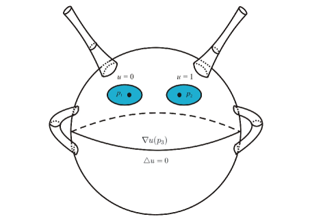
Fig. 2: The condenser method when $F^{-1}(\pi)$ is conformal to some twice punctured double torus.

Letting $\pi_{p}=T_{p}M^{2}$, one sees just as in section 4 that the assignment

$$M^{2}\ni p\to s(p)=DF(p_{3})\nabla u_{\pi_{p}}(p_{3})\in T_{p}M^{2}$$ (7.1)

defines a tangent vector field on $M^{2}$. A contradiction to $\chi(M^{2})\neq 0$ will follow as soon as we establish that this vector field is continuous and non-zero.

Proof of Theorem 4.2.The bulk of the proof is quite similar to the technical work done in section 5 to prove Theorem 4.1. In the interest of avoiding unnecessary duplication, we keep the same notation wherever possible and only concentrate on the steps where the argument needs to be modified. Notice that the definition of $s$ given in (7.1) is similar to (6.1).

One needs to establish the analogue of (6.2), where the point $b$ has been replaced by $p_{3}$. Keeping the same notation as in section 5, we let $\{K_{n}\}$ be an exhaustion of $\mathbb{R}^{n}$ by compact sets. Let $C_{1}$ be the connected component of $K_{1}\cap[F^{-1}(\pi)\setminus\overline{(U_{1}^{\pi_{z}}\cup U_{2}^{\pi_{z}})}]$ that contains $p_{3}=b$.

One can construct $\phi_{k}:C_{1}\to F^{-1}(\pi_{k})\subset\mathbb{R}^{n}$ as in (6.3). Lemma 6.1 is in force, and there is a smooth injection

$$\Psi:\overline{D}\to C_{1}\setminus{(U_{1}^{\pi_{z}}\cup U_{2}^{\pi_{z}})}$$

such that $\Psi(\overline{D})$ is disjoint from the boundaries $T_{1}^{\pi_{z}}$, $T_{2}^{\pi_{z}}$, and $\xi_{k}=\phi_{k}\circ\Psi$ satisfies $\xi_{k}(\overline{D})\subset F^{-1}(\pi)\setminus\overline{(U_{1}^{\pi_{z}}\cup U_{2}^{\pi_{z}})}$. Also, $d(T_{i}^{\pi_{k}},\xi_{k}(\overline{D}))>c_{1}>0,\;i=1,2$, where the constant $c_{1}$ is independent of all sufficiently large $k$.

By the maximum principle, $0\leq u_{\pi_{k}}\leq 1$ everywhere, and so there is no need to argue with the Harnack inequality. It follows directly from the interior estimate (6.8) that one can extract a subsequence of $(u_{\pi_{k}})$ so that the induced functions converge locally uniformly in the $C^{1}$ norm to a $\Delta_{\pi}$-harmonic function on $\Psi(\overline{D})$.

Next, one covers $C_{1}\setminus\overline{(U_{1}^{\pi_{z}}\cup U_{2}^{\pi_{z}})}$ with countably many sets $\Psi_{n}(\overline{D})$, where $\Psi_{1}=\Psi$ and, for $n>1$, $\Psi_{n}$ has similar properties. Working with convergent subsequences of functions (restricted to a larger set) of subsequences that were previously shown to be convergent on smaller sets, and then using the diagonal argument, as in the discussion preceding Lemma 6.2, one finally obtains a $\Delta_{\pi}$-harmonic function

$$\hat{u}_{\pi}:F^{-1}(\pi)\setminus\overline{(U_{1}^{\pi_{z}}\cup U_{2}^{\pi_{z}})}\to[0,1].$$

Using the boundary estimates (6.10), just as before, one can argue that $\hat{u}_{\pi}$ extends continuously to $T_{1}^{\pi_{z}}$, $T_{2}^{\pi_{z}}$ with boundary values $0$ and $1$, respectively. By the uniqueness of the solution of the Dirichlet problem, $\hat{u}_{\pi}=u_{\pi}$, and from this (6.2) follows, where $b$ has been replaced by $p_{3}$. Hence the continuity of $s$ has been established.

If one can argue that $\nabla u_{\pi_{p}}(p_{3})\neq 0$ for all $\pi_{p}$, $p\in M^{2}$, then by (7.1) the vector field $s$ would be not only continuous, but also zero-free, a contradiction to the Poincaré-Hopf theorem since $\chi(M^{2})\neq 0$.

As the ends of $F^{-1}(\pi_{p})$ are conformally punctured discs associated to the removable singularities of the $\underline{\rm bounded}$ harmonic function $u_{\pi_{p}}$, and doubly-connected planar regions are conformal to circular annuli, which are non-degenerate in the present context since they correspond to the complement of $U_{1}^{\pi_{p}}\cup U_{2}^{\pi_{p}}$ in the conformal compactification of $F^{-1}(\pi_{p})$, we only need to check the non-vanishing of $\nabla u$ when $u$ is the continuous function defined on the closed annulus $\{z\in\mathbb{C}:0<a<|z|\leq 1\}$ that is harmonic in its interior and satisfies $u=0$ ($u=1$) in the inner (outer) boundary circle. In this set-up the boundary circles correspond to $T_{1}^{\pi_{p}}$ and $T_{2}^{\pi_{p}}$. In other words, one only needs to deal with a standard condenser. But here the solution of the Dirichlet problem is quite explicit, namely:

$$u(z)=\frac{\log a-\log|z|}{\log a}.$$ (7.2)

Since $\nabla u\neq 0$ everywhere, $s$ would be continuous and nowhere zero, and the proof of Theorem 4.2 is complete.

∎

8 A general theorem and the inversion of polynomial maps

The following points about Theorems 4.1 and 4.2 are worth emphasizing:

a) Instead of endowing the domain $\mathbb{R}^{n}$ of $F$ with the standard flat metric, the proofs can be easily modified so as to allow for $F$ to be defined on any connected non-compact manifold $N^{n}$ carrying a Riemannian metric that induces on the surfaces $F^{-1}(\pi)$ the conformal type of $\mathbb{R}^{2}$ in Theorem 4.1, and that of a finitely punctured sphere in Theorem 4.2. b) The tangent bundle of $M^{2}$ was used only to the extent that one needed to guarantee that every continuous section $s$ (i.e. a vector field) must have a zero.

With remarks a) and b) in mind, we can state a general “abstract” theorem that subsumes both Theorems 4.1 and 4.2, as well as the algebraic result in [36] about the Jacobian conjecture (see Theorem 8.2 below). The proof of the result below involves only obvious adjustments of the proofs of the above mentioned theorems.

Theorem 8.1.

Let $N^{n}$ be a connected non-compact manifold, $F:N^{n}\to\mathbb{R}^{n}$ a local diffeomorphism, $n\geq 3$, $q\in F(N^{n})$. Assume the existence of a Riemannian metric $g$ on $N^{n}$, and a smooth vector bundle $T$ for which the following holds: i) Every fiber $\xi$ of $T$ belongs to $G_{2}(\mathbb{R}^{n})$ and the surface $F^{-1}(q+\xi)$ is conformally diffeomorphic, with respect to the metric induced by $g$, to a punctured sphere $S^{2}\setminus\{p_{1},\dots,p_{k(\xi)}\}$. ii) Every continuous section of $T$ has a zero. Then $F^{-1}(q)$ has one or two elements. The first alternative holds if $k(\xi)=1$ for every $\xi$.

There is a slight redundancy in the statement of Theorem 8.1, in the sense that the hypothesis $n\geq 3$ follows from i) and ii). Indeed, if $n=2$ the first half of i) implies that $T$ is the trivial bundle, contradicting ii).

In order to recover Theorems 4.1 and 4.2 from Theorem 8.1, it suffices to take $g$ to be the standard flat metric on $N^{n}=\mathbb{R}^{n}$, and for $T$ the tangent bundle of, say, an embedded sphere $S^{2}\subset\mathbb{R}^{n}$.

The invertibility criterion in (JC ) stated below, and alluded to in Example 2 of section 2, was first proved in [36]:

Theorem 8.2.

A polynomial local biholomorphism $F:\mathbb{C}^{n}\to\mathbb{C}^{n}$ is invertible if and only if for the generic point $q$ in $F(\mathbb{C}^{n})$ the following holds. For every complex line containing $q$ there is an open connected set $\mathcal{O}_{l}\subset\mathbb{R}^{2}$ that is homeomorphic to $F^{-1}(l)$.

Due to the polynomial nature of the map, the hypothesis is equivalent to asking that the pre-image of every complex line through $q$ be a connected rational curve, that is, $F^{-1}(l)$ should be conformal to $\mathbb{C}\mathbb{P}^{1}$ with finitely many points removed. This was the original formulation in [36].

To see this how Theorem 8.2 can be recovered from Theorem 8.1, assume that the pre-image of every complex line $\pi$ containing $0$, under a polynomial local biholomorphism $F:\mathbb{C}^{n}\to\mathbb{C}^{n}$, $n>1$, is a connected rational curve (there is no loss of generality in assuming that $0$ is a generic point in the image of $F$).

Endowing $\mathbb{C}^{n}$ with the flat metric arising from the identification of $\mathbb{C}^{n}$ with the Euclidean space $\mathbb{R}^{2n}$, any non-singular complex curve $C\subset\mathbb{C}^{n}$ will seemingly have two complex structures, the one inherited from the complex manifold $\mathbb{C}^{n}$, and a second one inherited from the Riemannian metric induced on $C$ by the standard Euclidean metric on $\mathbb{C}^{n}$. Using the Cauchy-Riemann equations and the fact that multiplication by $i$ induces an isometry in $\mathbb{C}^{n}$ one can check that these two complex structures coincide.

The complex lines through $q=0\in F(\mathbb{C}^{n})$ that are contained in a fixed $V\subset\mathbb{C}^{n}$, $V\approx\mathbb{C}^{2}$, are the fibers of the tautological line bundle $T$ over $\mathbb{C}\mathbb{P}^{1}$. Since $F^{-1}(l)$ is assumed to be connected for every complex line $l\subset V$, and $z\in F^{-1}(l)$ whenever $F(z)=0$, the manifold $N=F^{-1}(V)$ is likewise connected. Alternatively, $T$ can be viewed as a real bundle of rank two over $S^{2}$, so under the hypothesis of Theorem 8.2, condition i) in Theorem 8.1 holds. Since the Euler number of the tautological bundle is $-1$, hence non-zero, every continuous section of $T$ must vanish somewhere, so that hypothesis ii) also holds. Therefore, it follows from Theorem 8.1 that $\#F^{-1}(0)=1$ or $2$.

Fortunately, for algebraic reasons the generic fiber of a polynomial local biholomorphism cannot be $2$ (see Theorem 2.1 of [5], specifically the equivalence between statements a) and g)). Hence, $\#F^{-1}(0)=1$, and since $0$ is a generic point $F$ must be injective.

For polynomial local biholomorphisms injectivity implies surjectivity, and so the present proof of Theorem 8.2 is complete.

In the next section, we will prove a new theorem, similar in spirit to Theorem 8.2, but involving polynomial local biholomorphisms with real coefficients.

9 The condenser method in the presence of an involution

In the discussion at the beginning of section 7, if we had assumed that the pre-image of a plane $\pi$ was conformal to a connected finitely punctured surface of positive genus, the Dirichlet problem would still have a unique bounded solution $u_{\pi}$.

However, since the genus is positive, $\nabla u_{\pi}$ would necessarily have zeros. To see this, observe that after filling the punctures conformally the resulting manifold would be obtained form a compact Riemann surface of positive genus by the removal of two disjoint small discs. If the gradient of the solution of the Dirichlet problem had no zeros, the time $t$ map of the flow of the vector field

$$X(p)=\frac{\nabla u_{\pi}(p)}{|\nabla u_{\pi}(p)|^{2}},$$

where the norm comes from any Riemannian metric on the conformal compactification of $F^{-1}(\pi)$, applies any level set of $u_{\pi}$ onto another level set. Hence, for all all small $\epsilon>0$ the flow would take $\{u_{\pi}=\epsilon\}$ onto $\{u_{\pi}=1-\epsilon\}$, and so the compact surface with boundary would have been a topological cylinder $S^{1}\times[0,1]$, implying that the compactification of $F^{-1}(\pi)$ had genus zero.

Observe that the zero set of $\nabla u_{\pi}$ is discrete. Indeed, locally $u_{\pi}$ is the real part of a holomorphic function $h$ and, by the Cauchy-Riemann equations in local coordinates, $\nabla u_{\pi}$ can be identified with $\overline{h^{\prime}}$, with $h$ holomorphic. Since $u_{\pi}$ is non-constant, the zeros of $h^{\prime}$ are discrete, as desired.

Again referring to section 7, as the point $p_{3}$ lies in every $F^{-1}(\pi)$ one cannot guarantee a priori that $\nabla u_{\pi}(p_{3})\neq 0$ as one varies $\pi$ inside of a family of planes. In particular, if the genus of $F^{-1}(\pi)$ is positive it cannot be asserted that the (continuous) vector field defined in (7.1) is nowhere zero.

Nevertheless, as we shall see below, one can push further the conceptual connection between the Jacobian conjecture and the condenser method. In order to explain this, let us take $n=2$ and consider a polynomial local biholomorphism $F:\mathbb{C}^{2}\to\mathbb{C}^{2}$. If $F$ were to be a counterexample to (JC), the generic point would be covered at least three times [5, Theorem 2.1, equivalence a) $\Longleftrightarrow$ g)].

For notational simplicity, assume that $0$ is a generic point in the image of $F$. It is known that there are finitely many complex lines through $0$, say $l_{1},\dots,l_{k}$, with the property that the pre-image of every complex line $l\neq l_{j}$ is a connected finitely punctured compact Riemann surface of some fixed genus $g\geq 0$.

As remarked above, in the absence of injectivity the value $0$ would be covered three or more times. One can then use the condenser construction of section 7 to create a section

$$l\to s(l)=DF(p_{3})\nabla u_{l}(p_{3})\in l,$$

of the restriction of the tautological line bundle to the complement in $\mathbb{C}\mathbb{P}^{1}$ of the set $\Sigma=\{l_{1},\dots,l_{k}\}$ of exceptional lines. The analytic arguments from section 6 show that $s$ is continuous.

Multiplying $s$ by a smooth function on $\mathbb{C}\mathbb{P}^{1}$ that vanishes of a sufficiently high order at $\Sigma$, but is otherwise positive, one obtains a continuous section $\hat{s}$ of the actual tautological line bundle.

The zeros of $\hat{s}$ would occur at $\Sigma$, whenever this set is non-empty, as well as at the possible zeros of the original section $s$ constructed via the condenser method that might arise if the genus of the generic pre-image is positive, as explained before.

Assuming that $s$ has only finitely many zeros, the sum of the local indices of the singularities (zeros) of $\hat{s}$ would be $-1=$ the Euler number of the tautological bundle (see [25, p.133] for a general version of the Poincaré-Hopf theorem).

Progress in (JC) could conceivably be achieved if one had enough information about these local indices, so as to conclude that their sum could not be $-1$.

This contradiction would ensure that the pre-image of the generic point $0$ has at most two elements (recall that the condenser construction requires at least three points in the pre-image). But, as observed before [5, Thm.2.1], the cardinality of the generic fiber cannot be two, for algebraic reasons, and so the polynomial local biholomorphism would be injective.

For $n=2$ the proof of Theorem 8.2 follows precisely the outline given above, when the scenario is the simplest one possible. Indeed, under the hypotheses of Theorem 8.2 the pre-images of all complex lines are connected, so the exceptional lines $l_{j}$ would be absent from the above discussion. Also, since the pre-image of each complex line is supposed to be conformally a finitely punctured $\mathbb{C}\mathbb{P}^{1}$, the gradient of the harmonic function in the condenser construction has no zeros (see the discussion preceding (7.2)). Hence, $\hat{s}$ would be zero-free, an outright contradiction to the fact that the Euler number of the tautological bundle is non-zero.

In the absence of a technique for computing these local indices, we explore below a different line of argument, familiar in topological problems that can be approached using degree theory, where “symmetry” and “parity” replace the need to actually compute or estimate the local indices.

Specifically, since the Euler number of the tautological line bundle is $-1$, a contradiction also ensues in the preceding discussion if $\hat{s}$ is known to have an even number of singularities, grouped in pairs, whose indices are either pairwise equal or differ by a sign. Indeed, the sum of the indices would be zero mod (2). The preceding discussion provides the heuristics for the main result of this section.

It will be observed in Lemma 9.5 that if $F:\mathbb{C}^{n}\to\mathbb{C}^{n}$, $n\geq 2$, is a polynomial local biholomorphism with $\underline{\rm real}$ coefficients, and $\Sigma\subset\mathbb{C}^{n}$ is any complex algebraic hypersurface, then $F(\mathbb{R}^{n})$ is not contained in $\Sigma$. This allows us to make sense of the expression “a generic point in $F(\mathbb{R}^{n})$”, which is part of the hypotheses of the theorem below.

Theorem 9.1.

A polynomial local biholomorphism $F:\mathbb{C}^{n}\to\mathbb{C}^{n}$ that commutes with conjugation is invertible if and only if for the generic point $q\in F(\mathbb{R}^{n})\subset\mathbb{R}^{n}$ the following holds: For every complex line $l$ containing $q$ that is invariant under conjugation there is an open connected set $\mathcal{O}_{l}\subset\mathbb{R}^{2}$ such that $F^{-1}(l)$ is homeomorphic to $\mathcal{O}_{l}$.

Here, it is meant that the complex line $l\subset\mathbb{C}^{n}$ is invariant under conjugation as a set, and not in the pointwise sense. In $\mathbb{C}^{2}$ such a line is the zero set of a linear equation with real coefficients. Commutation of $F$ with conjugation follows if the components of $F$ are polynomials with real coefficients coefficients.

Since $F$ is a polynomial map, the topological assumption in the statement of the theorem implies that $\mathcal{O}_{l}$ is conformal to $\mathbb{C}\mathbb{P}^{1}$ punctured a finite number $n_{l}$ of times, i.e. $F^{-1}(l)$ is a connected rational curve.

Remark 9.2.

Theorem 9.1 invites comparison with Theorem 8.2. In the latter, injectivity is achieved if the pre-images of all complex lines $l$ through a generic point of $F(\mathbb{C}^{n})$ are homeomorphic to planar domains. In Theorem 9.1, where the coefficients of the map are real, accordingly, in order to obtain injectivity one only needs that the pre-images of all complex lines given by linear equations with real coefficients, and passing through a generic point in $F(\mathbb{R}^{n})$, be homeomorphic to planar domains.

One should stress that the hypotheses of Theorem 9.1 impose no restrictions on the topology of the pre-images of those complex lines that are not invariant under complex conjugation.

Remark 9.3.

As observed by several authors, the Jacobian conjecture holds if and only if injectivity can be established in all dimensions for those polynomial local biholomorphisms of $\mathbb{C}^{n}$ into itself that have $\underline{\rm real}$ coefficients.

Indeed, if $F:\mathbb{C}^{n}\to\mathbb{C}^{n}$ is polynomial and $\text{det}DF=1$, its realification $\widehat{F}:\mathbb{R}^{2n}\to\mathbb{R}^{2n}$ satisfies

$$\text{det}D\widehat{F}(p)=|\text{det}DF(p)|^{2}=1.$$

(More generally, this relation holds for all holomorphic maps $F:\mathbb{C}^{n}\to\mathbb{C}^{n}$.) The complexification $\widetilde{F}:\mathbb{C}^{2n}\to\mathbb{C}^{2n}$ of $\widehat{F}$ has real coefficients and satisfies $\text{det}D\widetilde{F}=1$. Clearly, if $\widetilde{F}$ is injective so are, in succession, $\widehat{F}$ and $F$.

Note, however, that Theorems 8.2 and 9.1 are logically independent invertibility criteria.

Before commencing the proof of Theorem 9.1, we make some elementary observations that will also help us fix the notation. If $\mathbb{C}^{2}$ is given coordinates $(z,w)$, the complex lines through $0$ are of the form $z=0$ and $w=\alpha z$, with $\alpha\in\mathbb{C}$, and so they are identified with the points in $\mathbb{C}\mathbb{P}^{1}$ given in homogeneous coordinates by $(0:1)$ and $(1:\alpha)$, $\alpha\in\mathbb{C}$.

The tautological line bundle $T$, when restricted to the affine part of $\mathbb{C}\mathbb{P}^{1}$, associates to $\alpha\in\mathbb{C}$ the complex line given by $w=\alpha z$. Hence, $\xi(\alpha)=(1,\alpha)$, $\alpha\in\mathbb{C}$, defines a section of the restriction $T|\mathbb{C}$. The Euler number $e(T)$ of the tautological line bundle is the local index of $\xi$ at its singularity at infinity.

Introducing a new coordinate $\zeta=1/\alpha$, $|\zeta|\leq 1$, the index at infinity can be computed as the local index at $0$ of the section $\zeta\to(1,1/\zeta)=(1,\overline{\zeta}/|\zeta|^{2})$, and so $e(T)=-1$.

Complex conjugation acts not only on $\mathbb{C}^{2}$, but on $\mathbb{C}\mathbb{P}^{1}$ as well, via $\overline{(z:w)}=(\overline{z}:\overline{w})$. The real projective line $\mathbb{R}\mathbb{P}^{1}$ can be identified with the maximal subset of $\mathbb{C}\mathbb{P}^{1}$ that is left pointwise invariant under conjugation, namely

$$\mathbb{R}\mathbb{P}^{1}\cong\{(1:x)\;|\;x\in\mathbb{R}\}\cup\{(0:1)\}.$$

Indeed, if $\overline{(z:w)}=(z:w)$, with $z\neq 0$, one has $\frac{w}{z}=\frac{\overline{w}}{\overline{z}}=\overline{(\frac{w}{z})}=x\in\mathbb{R}.$ In particular, $(z:w)=(z:xz)=(1:x).$

Identifying $\mathbb{C}\mathbb{P}^{1}$ with the unit sphere $S^{2}$ given by $x^{2}+y^{2}+t^{2}=1$ in $\mathbb{R}^{3}$ endowed with coordinates $(x,y,t)$, $z=x+iy$, and then using stereographic projection from the north pole $(0,0,1)$, one sees that $\mathbb{R}\mathbb{P}^{1}$ can be identified with the intersection of $S^{2}$ and the plane $y=0$. Hence, $\mathbb{C}\mathbb{P}^{1}\setminus\mathbb{R}\mathbb{P}^{1}=D^{+}\cup D^{-},$ where $D^{+}$ and $D^{-}$ are disjoint topological discs, intertwined under conjugation, corresponding in the affine part of $\mathbb{C}\mathbb{P}^{1}$ to the sets $\{z\in\mathbb{C}\;|\text{Im}z>0\}$ and $\{z\in\mathbb{C}\;|\text{Im}z<0\}$.

Besides the ordinary complex tautological complex line bundle $T$ over $\mathbb{C}\mathbb{P}^{1}$, one has in a natural way a tautological real line bundle over $\mathbb{R}\mathbb{P}^{1}$. Namely, one associates to $(0:1)$ and $(1:\beta)$, where $\beta\in\mathbb{R}$, the lines in $\mathbb{R}^{2}$ given by $x=0$ and $y=\beta x$. We denote this real line bundle by $T_{\mathbb{R}}$. Abusing the notation somewhat, we bypass the canonical projection and, for a given complex line $l$ in $\mathbb{C}^{2}$ that passes through $0$, we write both $l\subset\mathbb{C}^{2}$ and $l\in\mathbb{C}\mathbb{P}^{1}$. Let $T_{0}$ be the restriction of $T$ to $\mathbb{R}\mathbb{P}^{1}$.

It is clear that a section $\xi_{0}$ of $T_{0}$ that satisfies $\xi_{0}(l)=\overline{\xi_{0}(l)}$ for every $l\in\mathbb{R}\mathbb{P}^{1}$ induces a section of $T_{\mathbb{R}}$, and vice versa. Since $T_{\mathbb{R}}$ is a real line bundle over $\mathbb{R}\mathbb{P}^{1}\approx S^{1}$, it is isomorphic to either the trivial bundle or the Möbius bundle. It follows from the lemma below that the second alternative holds.

Lemma 9.4.

Every continuous section of $T_{\mathbb{R}}$ vanishes somewhere in $\mathbb{R}\mathbb{P}^{1}$. Otherwise said, if $\xi_{0}$ is a continuous section of $T_{0}$ that satisfies $\xi_{0}(l)=\overline{\xi_{0}(l)}$ for all $l\in\mathbb{R}\mathbb{P}^{1}$, then $\xi_{0}$ must have a zero on $\mathbb{R}\mathbb{P}^{1}$.

To prove this lemma, suppose by contradiction that $\xi_{0}$ vanishes nowhere on $\mathbb{R}\mathbb{P}^{1}$. One can extend $\xi_{0}$ continuously to a section $\xi_{0}^{+}$ of the restriction $T|D^{+}$, smooth outside a half-collar of $\mathbb{R}\mathbb{P}^{1}$ in $D^{+}$, and which, by transversality, has only finitely many zeros on $D^{+}$. Having obtained $\xi_{0}^{+}$, we now define a section $\xi_{0}^{-}$ on $D^{-}$ by “reflection”, setting

$$\xi_{0}^{-}(l)=\overline{\xi_{0}^{+}(\overline{l})},\;\;l\in D^{-}.$$ (9.1)

Consider the section $\xi$ of $T$ defined to be $\xi_{0}^{+}$ on $D^{+}$, $\xi_{0}^{-}$ on $D^{-}$, and $\xi_{0}$ on $\mathbb{R}\mathbb{P}^{1}$. Since $\mathbb{R}\mathbb{P}^{1}$ is kept pointwise fixed under conjugation, the hypothesis of the lemma and (9.1) imply that $\xi$ is continuous. Since we are assuming that $\xi_{0}$ has no zeros on $\mathbb{R}\mathbb{P}^{1}$, the zeros of $\xi$, if any, must lie in $D^{+}\cup D^{-}$ and occur in pairs, one in $D^{+}$ and the other in $D^{-}$. One can check using (9.1) that the local indices are pairwise the same.

To see this, denote by $\Lambda$ the action of complex conjugation on $\mathbb{C}\mathbb{P}^{1}$, so that $\Lambda(l)=\overline{l}$. One can rewrite (9.1) as

$$\xi_{0}^{-}=\Lambda\circ\xi_{0}^{+}\circ\Lambda.$$ (9.2)

If $l_{0}$ is a zero of $\xi_{0}^{-}$ then $\Lambda(l_{0})$ is a zero of $\xi_{0}^{+}$, and vice versa. Keeping in mind that in the natural local coordinates $\Lambda$ is a real linear involution, so that $\Lambda^{-1}=\Lambda$ and $d\Lambda(l_{o})=\Lambda$, one can rewrite (9.2) as

$$\xi_{0}^{-}(l)=\Lambda(\xi_{0}^{+}(\Lambda(l)))=\big{[}d\Lambda(\l)\big{]}^{-1}(\xi_{0}^{+}(\Lambda(l)).$$ (9.3)

The last relation displays the section $\xi_{0}^{-}$ as the pull-back of $\xi_{0}^{+}$ under $\Lambda$. In particular,

$$\text{Ind}(\xi_{0}^{-},l_{0})=\text{Ind}(\xi_{0}^{+},\Lambda(l_{0})).$$ (9.4)

Hence, as claimed, the zeros of $\xi$ occur in pairs, and the zeros in a given pair have the same local index. It follows that the sum of all local indices is $0$ mod (2), contradicting the fact that the Euler number of $T$ is $-1$. This concludes the proof of the lemma.

To prove Theorem 9.1 we will argue by contradiction, using the solutions of the Dirichlet problems from section 6 in order to create a section $\xi_{0}$ of $T_{\mathbb{R}}$ that violates Lemma 9.4. But before we can achieve this, we need to prove one more lemma. For the sake of completeness, we include its proof.

Lemma 9.5.

Let $F:\mathbb{C}^{n}\to\mathbb{C}^{n}$ be a polynomial local biholomorphism with real coefficients, $n\geq 2$, and $\Sigma$ a complex hypersurface. Then $F(\mathbb{R}^{n})\cap[\mathbb{R}^{n}\setminus\Sigma]\neq\emptyset$.

Proof.

Assume by contradiction that $F(\mathbb{R}^{n})\subset\Sigma$, so that

$$\mathbb{R}^{n}\subset\Sigma_{1}\stackrel{{\scriptstyle def}}{{=}}F^{-1}(\Sigma).$$ (9.5)

Let $\Sigma_{2}$ be the singular set of the complex algebraic variety $\Sigma_{1}$, $\Sigma_{3}$ the singular set of $\Sigma_{2}$, and so on. One then has a descending chain of inclusions

$$\Sigma_{1}\supset\Sigma_{2}\supset\Sigma_{3}\supset\cdots\supset\Sigma_{r-1}\supset\Sigma_{r},$$ (9.6)

where $r\geq 1$ and $\Sigma_{r}$ is smooth and closed in $\mathbb{C}^{n}$. From $(\ref{inclusion})$ and $(\ref{chain})$ we can write

$$\mathbb{R}^{n}=\mathbb{R}^{n}\cap\Sigma_{1}=\big{[}\mathbb{R}^{n}\cap(\Sigma_{1}\setminus\Sigma_{2})\big{]}\cup\cdots\cup\big{[}\mathbb{R}^{n}\cap(\Sigma_{r-1}\setminus\Sigma_{r})\big{]}\cup\big{[}\mathbb{R}^{n}\cap\Sigma_{r}\big{]}.$$ (9.7)

By the Baire category theorem, the closure in $\mathbb{R}^{n}$ of at least one of the sets in the brackets on the right hand side of the above decomposition has non-empty interior in $\mathbb{R}^{n}$.

We distinguish between two cases (notation: the symbol int refers to the operation of taking the interior of a set in $\mathbb{R}^{n}$, whereas the bar stands for the operation of taking closure in $\mathbb{R}^{n}$): a) $\text{int}\overline{(\mathbb{R}^{n}\cap\Sigma_{r}])}\neq\emptyset$. b) $\text{int}\overline{\big{[}\mathbb{R}^{n}\cap(\Sigma_{i}\setminus\Sigma_{i+1})\big{]}}\neq\emptyset$, for some $i=1,\dots,r-1$.

We treat b) first. Choose $j$ to be the largest index $\leq r-1$ for which

$$\text{int}\overline{\big{[}\mathbb{R}^{n}\cap(\Sigma_{j}\setminus\Sigma_{j+1})\big{]}}\neq\emptyset.$$

Since $\mathbb{R}^{n}$, $\Sigma_{j}$ are both closed in $\mathbb{C}^{n}$, and $\Sigma_{j+1}$ has empty interior in $\Sigma_{j}$, the last condition and the maximality of $j$ imply

$$\text{int}[\mathbb{R}^{n}\cap\Sigma_{j}]\neq\emptyset,\;\;\;\;\text{int}[\mathbb{R}^{n}\cap\Sigma_{j+1}]=\emptyset.$$ (9.8)

By the first half of (9.8) there exist $z\in\mathbb{R}^{n}\cap\Sigma_{j}$ and $\epsilon>0$ such that the open ball $B(z,\epsilon)$ in $\mathbb{R}^{n}$ satisfies $B(z,\epsilon)\subset\Sigma_{j}.$

If $z\in\Sigma_{j}\setminus\Sigma_{j+1}$, set $z^{\prime}=z$ and choose $\epsilon^{\prime}$ such that $0<\epsilon^{\prime}<\min\{\epsilon,d(z^{\prime},\Sigma_{j+1})\}$, where $d$ stands for the Euclidean distance, so that $B(z^{\prime},\epsilon^{\prime})\subset\Sigma_{j}\setminus\Sigma_{j+1}$.

If $z\in\Sigma_{j+1}$, then by the second half of (9.8) one has $\text{int}[B(z,\epsilon)\cap\Sigma_{j+1}]=\emptyset,$ in which case there exists $z^{\prime}\in B(z,\epsilon)\cap(\Sigma_{j}\setminus\Sigma_{j+1})$ and some $\epsilon^{\prime}>0$ such that $B(z^{\prime},\epsilon^{\prime})\subset\Sigma_{j}\setminus\Sigma_{j+1}$.

Thus, in both cases above the point $z^{\prime}$ is the center of a ball in $\mathbb{R}^{n}$ that is fully contained in the regular set $\Sigma_{j}\setminus\Sigma_{j+1}$.

Looking at tangent spaces, one has $\mathbb{R}^{n}\subset T_{\mathbb{C},z^{\prime}}(\Sigma_{j}).$ But $T_{\mathbb{C},z^{\prime}}(\Sigma_{j})$ is invariant under multiplication by $i$, so that $\mathbb{C}^{n}=\mathbb{R}^{n}+i\mathbb{R}^{n}\subset T_{\mathbb{C},z^{\prime}}(\Sigma_{j})$, implying that

$$n=\text{dim}\Sigma_{j}\leq\text{dim}\Sigma_{1}=n-1,$$

a contradiction. This completes the proof of Lemma 9.5 under alternative b).

If alternative a) is in force one has $\text{int}(\Sigma_{r})\neq\emptyset$, and since $\Sigma_{r}$ is smooth we also obtain a ball $B(z^{\prime},\epsilon^{\prime})$ in $\mathbb{R}^{n}$ that is fully contained in the non-singular variety $\Sigma_{r}$. The argument in the previous paragraph, involving tangent spaces, leads to $n=\text{dim}\Sigma_{r}\leq\text{dim}\Sigma_{1}=n-1$, a contradiction. This concludes the proof of Lemma 9.5.

∎

It is well known that under the hypotheses of the Jacobian Conjecture there exists a complex algebraic hypersurface $\Sigma\subset\mathbb{C}^{n}$, perhaps with singularities, for which the restriction $\mathbb{C}^{n}\setminus F^{-1}(\Sigma)\stackrel{{\scriptstyle F}}{{\to}}\mathbb{C}^{n}\setminus\Sigma$ is a cover map.

Continuing with the proof of Theorem 9.1, by Lemma 9.5 we can choose a point $q$ in $\mathbb{R}^{n}\setminus\Sigma$ of the form $q=F(p_{3})$, where $\overline{p}_{3}=p_{3}$, i.e. $p_{3}\in\mathbb{R}^{3}$.

Let $V=\mathbb{C}^{2}\subset\mathbb{C}^{n}$ (natural inclusion), and $V^{\prime}=q+V$. If $l$ is a complex line through $q\in\mathbb{R}^{n}$ that is contained in $V^{\prime}$ and is invariant under conjugation then, by hypothesis, $F^{-1}(l)$ is connected and contains $p_{3}$. In particular, $N=F^{-1}(V^{\prime})$ is connected as well.

Suppose, by way of contradiction, that $F$ is not injective. Since, as observed in section 7, the generic fiber of $F$ must have cardinality at least three, and $q\notin\Sigma$, there are points $p_{1},p_{2}\in N$ such that $p_{1}$, $p_{2}$, $p_{3}$ are all distinct and $F(p_{j})=q$, $j=1,2,3$. If $F(z)=q$, then $F(\overline{z})=\overline{F(z)}=\overline{q}=q$. Thus, one can assume that:

($\bullet$) Either both $p_{1}$ and $p_{2}$ belong to $\mathbb{R}^{n}$, or both $p_{1}$ and $p_{2}$ belong to $\mathbb{C}^{n}\setminus\mathbb{R}^{n}$ and $\overline{p}_{1}=p_{2}$.

Let $W$ be an Euclidean ball in $\mathbb{C}^{n}$, centered at $q$, and $U_{1},U_{2}$ the corresponding disjoint neighborhoods of $p_{1}$ and $p_{2}$ that are mapped biholomorphically onto $W$.

The complex lines $l$ in $V^{\prime}$ that contain $q$ can be naturally identified with $\mathbb{C}\mathbb{P}^{1}$. Likewise, recalling that $q\in\mathbb{R}^{n}$, those complex lines in $V^{\prime}$ that contain $q$ and are invariant under conjugation are naturally identified with $\mathbb{R}\mathbb{P}^{1}\subset\mathbb{C}\mathbb{P}^{1}$.

Given $l\in\mathbb{R}\mathbb{P}^{1}$, write $U_{1}^{l},U_{2}^{l}$ for the intersections of the neighborhoods $U_{1},U_{2}$ with $F^{-1}(l)$, and set $T_{i}^{l}=\partial U_{i}^{l}$ (the boundary is taken in $F^{-1}(l)$), $i=1,2$.

Arguing as in section 6, there is a unique bounded harmonic function $u_{l}$ defined in the complement of the closure of $U_{1}^{l}\cup U_{2}^{l}$ in the finitely punctured compact Riemann surface $F^{-1}(l)$ that extends continuously to $T_{1}^{l}\cup T_{2}^{l}$ and satisfies

$$u_{l}|T_{1}^{l}=0,\;\;\;u_{l}|T_{2}^{l}=1.$$

As observed in ($\bullet$), either $p_{1},\;p_{2}\in\mathbb{R}^{n}$, or $p_{1},\;p_{2}\in\mathbb{C}^{n}\setminus\mathbb{R}^{n},\overline{p}_{1}=p_{2}$. We will show that

Lemma 9.6.

If the radius of the Euclidean ball $W$ is sufficiently small and $l\in\mathbb{R}\mathbb{P}^{1}$, then $F^{-1}(l)=\overline{F^{-1}(l)}$. Furthermore, a) If $p_{1},p_{2}\in\mathbb{R}^{n}$, then

$$U_{j}^{l}=\overline{(U_{j}^{l})},\;\;\;T_{j}^{l}=\overline{(T_{j}^{l})},\;\;\;j=1,2.$$ (9.9)

b) If $p_{1},p_{2}\in\mathbb{C}^{n}\setminus\mathbb{R}^{n}$, $\overline{p}_{1}=p_{2}$, then

$$U_{1}^{l}=\overline{(U_{2}^{l})},\;\;\;T_{1}^{l}=\overline{(T_{2}^{l})}.$$ (9.10)

We proceed with the proof of Lemma 9.6. By hypothesis, $F(\overline{z})=\overline{F(z)}$ ($F$ has real coefficients) and $\overline{l}=l$. Also, we chose $W$ to be an Euclidean ball centered at $q\in\mathbb{R}^{n}\setminus\Sigma$, $W\cap\Sigma=\emptyset$, so that $W=q+W_{0}$ where $W_{0}$ is an Euclidean ball centered at $0$. In particular, since conjugation is an Euclidean isometry, $\overline{W}_{0}=W_{0}$. Hence, since $q\in\mathbb{R}^{n}$, one has

$$\overline{W}=\overline{(q+W_{0})}=\overline{q}+\overline{W_{0}}=q+W_{0}=W.$$

In order to establish the relation $F^{-1}(l)=\overline{F^{-1}(l)}$, observe

$$z\in F^{-1}(l)\Leftrightarrow\overline{F(z)}\in\overline{l}\Leftrightarrow F(\overline{z})\in l\Leftrightarrow\overline{z}\in F^{-1}(l)\Leftrightarrow z\in\overline{F^{-1}(l)}.$$

Since $\mathbb{C}^{n}\setminus F^{-1}(\Sigma)\stackrel{{\scriptstyle F}}{{\to}}\mathbb{C}^{n}\setminus\Sigma$ is a finite covering, say of degree $N$, if the radius of $W$ is small enough then

$$F^{-1}(W\cap l)=\bigcup_{n=1}^{N}U_{n}^{l},$$ (9.11)

where the $U_{n}^{l}$ are pairwise disjoint and are applied biholomorphically by $F$ onto $W\cap l$. To establish $U_{1}^{l}=\overline{U_{1}^{l}}$ in (9.10), and similarly for $U_{2}^{l}$, observe that

$$z\in U_{1}^{l}\Rightarrow F(\overline{z})=\overline{F(z)}\in\overline{F(U_{1}^{l})}=\overline{W\cap l}=W\cap l\Rightarrow\overline{z}\in F^{-1}(W\cap l)=\bigcup_{n=1}^{N}U_{n}^{l}.$$ (9.12)

For each $n$, the set $A_{n}=\{z\in U_{1}^{l}:\overline{z}\in U_{n}^{l}\}$ is open in $U_{1}^{l}$, $A_{n}\cap A_{m}=\emptyset$ if $n\neq m$ and, by (9.12), $U_{1}^{l}=\cup_{n=1}^{N}A_{n}$. By connectedness, there exists a unique $n\geq 1$ such that $U_{1}^{l}=A_{n}$, so that $U_{1}^{l}=\overline{U_{n}^{l}}$. Similarly, there is a unique integer $m$ such that $U_{2}^{l}=\overline{U_{m}^{l}}$. Since $p_{1}$, $p_{2}$ belong to $\mathbb{R}^{n}$, $U_{1}^{l}\cap\overline{U_{1}^{l}}\neq\emptyset$ and $U_{2}^{l}\cap\overline{U_{2}^{l}}\neq\emptyset$. Hence, $n=m=1$ and so $U_{1}^{l}=\overline{U_{1}^{l}}$, $U_{2}^{l}=\overline{U_{2}^{l}}$. The proof of $T_{j}^{l}=\overline{(T_{j}^{l})},\;\;\;j=1,2$ runs along similar lines. This concludes the proof of a).

For the proof of b) one follows the above arguments up to the existence of a unique $n$ such that $U_{1}^{l}=\overline{U_{n}^{l}}$. As we are assuming $p_{1},p_{2}\in\mathbb{C}^{n}\setminus\mathbb{R}^{n}$, $\overline{p}_{2}=p_{1}$, the intersection $U_{1}^{l}\cap\overline{U_{2}^{l}}$ is non-empty, and therefore one has $U_{1}^{l}=\overline{(U_{2}^{l})}$. In a similar way one obtains $T_{1}^{l}=\overline{(T_{2}^{l})}.$ This concludes the proof of Lemma 9.6.

To continue with the proof of Theorem 9.1, assume first that $p_{1},p_{2}\in\mathbb{R}^{n}$ and for $l\in\mathbb{R}\mathbb{P}^{1}$ consider the function

$$v_{l}:F^{-1}(l)\setminus(U_{1}^{l}\cup U_{2}^{l}),\;\;v_{l}(z)=u_{l}(\overline{z}).$$

That $v_{l}$ is well-defined follows from (9.9). Writing $z=\phi(\zeta)\in F^{-1}(l)\setminus\overline{(U_{1}^{l}\cup U_{2}^{l})}$, where $\phi$ is a local holomorphic coordinate, and observing that the composition of a harmonic function with an anti-holomorphic function is still harmonic, one sees that $v_{l}$ is harmonic in the interior of its domain.

Using (9.9) again, one sees that $v_{l}$ extends continuously to the boundary with values $0$ and $1$ on $T_{1}^{l}$ and $T_{2}^{l}$, respectively. By the uniqueness of the solution of the Dirichlet problem, it follows that $v_{l}=u_{l}$. Hence, for all $z$ in the domain of $u_{l}$, i.e. $F^{-1}(l)\setminus{(U_{1}^{l}\cup U_{2}^{l})}$, one has

$$u_{l}(z)=u_{l}(\overline{z}).$$ (9.13)

If $\overline{l}=l$ and $\beta:(-\epsilon,\epsilon)\to F^{-1}(l)\setminus\overline{(U_{1}^{l}\cup U_{2}^{l})}$ is a smooth curve with $\beta(0)=z$ and $\beta^{\prime}(0)=w$, differentiation of $u_{l}(\beta(t))=u_{l}(\overline{\beta(t)})$ yields $du_{l}(z)w=du_{l}(\overline{z})\overline{w}.$ Equivalently, since conjugation is an Euclidean isometry,

$$\langle\nabla u_{l}(z),w\rangle=\langle\nabla u_{l}(\overline{z}),\overline{w}\rangle=\langle\overline{\nabla u_{l}(\overline{z})},w\rangle.$$

As $w$ is arbitrary, this implies $\nabla u_{l}(z)=\overline{\nabla u_{l}(\overline{z})}$, and so

$$\overline{\nabla u_{l}(z)}={\nabla u_{l}(\overline{z})},\;\;\;\overline{l}=l.$$ (9.14)

Set $\xi_{0}(l)=DF(p_{3})\nabla u_{l}(p_{3})$, $l\in\mathbb{R}\mathbb{P}^{1}$. It follows from the proof of Theorem 4.2 in section 6 that $\xi_{0}$ is continuous. Also, since $F^{-1}(l)$ is conformal to a finitely punctured $\mathbb{C}\mathbb{P}^{1}$, $\xi_{0}$ is nowhere zero.

Recalling that $\overline{p}_{3}=p_{3}$ and $\overline{l}=l$, we have, after using (9.14) and the fact that the matrix $DF(p_{3})$ has real entries because the components of $F$ have real coefficients:

$$\overline{\xi_{0}(l)}=\overline{DF(p_{3})\nabla u_{l}(p_{3})}=\overline{DF(p_{3})}\;\;\overline{\nabla u_{l}(p_{3})}=DF(p_{3})\nabla u_{l}(\overline{p_{3}})=DF(p_{3})\nabla u_{l}(p_{3})=\xi_{0}(l).$$

As $\xi_{0}$ is continuous and nowhere zero, this contradicts Lemma 9.4. This concludes the proof of Theorem 9.1 under the assumption that $p_{1},p_{2}\in\mathbb{R}^{n}$.

Let us now deal with the remaining alternative, namely $p_{1}=\overline{p_{2}}$. In this case, conjugation switches the $U^{\prime}s$ and the $T^{\prime}s$. More precisely, by (9.10) we have $U_{1}^{l}=\overline{(U_{2}^{l})},T_{1}^{l}=\overline{(T_{2}^{l})}$.

If we consider the function $v_{l}$ to be defined as before, $v_{l}(z)=u_{l}(\overline{z})$, then $v$ would be harmonic but the boundary conditions $0$ and $1$ would not correspond to the same boundary components as the original function $u$. In particular, one cannot use the uniqueness of solutions of the Dirichlet problem to conclude that $u_{l}$ and $v_{l}$ are the same.

To circumvent this difficulty, in the case where $p_{1}=\overline{p_{2}}$ we define a $\underline{\rm new}$ $v_{l}$ by

$$v_{l}(z)=1-u_{l}(\overline{z}).$$ (9.15)

It is now clear that $u_{l}$ and $v_{l}$ are harmonic and have the same boundary values. By uniqueness, $u_{l}=v_{l}$, and so

$$u_{l}(z)=1-u_{l}(\overline{z}).$$ (9.16)

In particular, if $z=\overline{z}$ lies in the domain of $u$ one has $u(z)=\frac{1}{2}$ and therefore we are dealing with a level line. Since $F^{-1}(l)$ is conformally a punctured sphere, $\nabla u_{l}$ never vanishes and is perpendicular to the above level line, whereas $i\nabla u_{l}$ is tangent. With this in mind, we define a new $\xi_{0}$ by setting

$$\xi_{0}(l)=DF(p_{3})i\nabla u_{l}(p_{3})=iDF(p_{3})\nabla u_{l}(p_{3}),\;l\in\mathbb{R}\mathbb{P}^{1}.$$ (9.17)

The second equality follows because $F$ is holomorphic. Repeating the arguments given after (9.13), but using (9.16) as the starting point instead of $u_{l}(z)=u_{l}(\overline{z})$ , we obtain

$$\overline{\nabla u_{l}(z)}=-\nabla u_{l}(\overline{z})$$ (9.18)

To finish the proof, we must establish $\xi_{0}(l)=\overline{\xi_{0}(l)}$ whenever $l=\overline{l}$. To check this, use $p_{3}=\overline{p_{3}}$, (9.17) and (9.18), to see that $\overline{\xi_{0}(l)}$ equals

$$\overline{DF(p_{3})i\nabla u_{l}(p_{3})}=(-i)\overline{DF(p_{3})}\;\;\overline{\nabla u_{l}(p_{3})}=(-i)DF(p_{3})(-1)\nabla u_{l}(\overline{p_{3}})=iDF(p_{3})\nabla u_{l}(p_{3}),$$

And so $\xi_{0}(l)=\overline{\xi_{0}(l)}$ whenever $l=\overline{l}$, as desired. As before, this contradicts Lemma 9.4, and the proof of Theorem 9.1 is finished.

10 A conjecture in approximation theory

In this section we make some observations concerning the Jacobian conjecture and its relation to the ideas discussed in this paper.

In the absence of a proof that polynomial local biholomorphisms are injective, one might want to aim for a less ambitious goal, and try to settle the question at the “next level” of difficulty. Namely, one would like to show at least that, under the assumptions of (JC), the pre-images of all complex lines are connected.

This can be thought of as a “vestigial” form of injectivity, since actual injectivity means that the pre-images of all points are connected (see section 2). Note that, as discussed in Example 5, subsection 2.5, the pre-images of all real hyperplanes are always connected in the (JC) setting.

However, even the simpler problem of showing that all complex lines in $\mathbb{C}^{2}$ in a family of parallel lines pull-back into connected complex curves seems to be open at this time. More precisely, if $(f,g):\mathbb{C}^{2}\to\mathbb{C}^{2}$ is as in the Jacobian conjecture then, to the best of our knowledge, it is only known that the curve $f+c=0$ is connected for all but at most finitely many values of $c\in\mathbb{C}$.

Equivalently, one would like to show at least that if $(f,g)$ is any Jacobian pair, then $f$ and $g$ are irreducible polynomials. Given its seemingly simpler nature, solving this last problem in the affirmative would be a reasonable litmus test for the veracity of the Jacobian Conjecture.

The techniques in this paper, meant to deal with the less restrictive case of injectivity of local diffeomorphisms, offer no indication of why (JC) should hold. Be that as it may, our results actually hint, ever so gently, at the possibility that (JC) might actually be false. Indeed, the potential lack of connectedness of the pre-images of complex lines, and the possibility that even if these complex curves are connected they may have positive genera, appear as major stumbling blocks.

Various conjectures have been formulated over the years whose validity would imply that of (JC). Here, in view of the previous comments, we go in the opposite direction by formulating a natural conjecture in approximation theory which, if true, would imply that (JC) $\underline{\rm fails}$, in principle without the onus of having to exhibit a counterexample. The new viewpoint is conceptually related to the simple fact that any holomorphic map $\mathbb{C}^{n}\to\mathbb{C}^{n}$ can be uniformly approximated, over any given compact subset, by polynomial maps.

We juxtapose (JC) to the new conjecture, in case the reader feels inclined to ponder if one statement is more likely to be true than the other. The Jacobian conjecture. Every polynomial map $F:\mathbb{C}^{n}\to\mathbb{C}^{n}$, $n\geq 1$, with constant non-zero Jacobian determinant is injective. The polynomial approximation conjecture. Every holomorphic map $G:\mathbb{C}^{n}\to\mathbb{C}^{n}$, $n\geq 1$, with constant non-zero Jacobian determinant can be uniformly approximated over compact subsets by polynomial maps $F:\mathbb{C}^{n}\to\mathbb{C}^{n}$ with constant non-zero Jacobian determinant. When $n=1$ both statements are trivially true. To see why the validity of the second conjecture, for some $n\geq 2$, implies that (JC) is false, observe that in finite dimensions if a sequence of injective local diffeomorphisms converges uniformly over compact subsets to a local diffeomorphism, then the limit map is also injective (an easy argument using degree theory can be found in [43, p.411]).

Since the obviously non-injective map $G:\mathbb{C}^{2}\to\mathbb{C}^{2}$, $G(z_{1},z_{2})=(e^{z_{1}},z_{2}e^{-z_{1}})$, has Jacobian determinant one (similarly for $G(z_{1},\dots,z_{n})=(e^{z_{1}},z_{2}e^{-z_{1}},z_{3},\dots,z_{n})$ when $n\geq 3$), the tail of a hypothetical sequence of polynomial local biholomorphisms converging uniformly to $G$ over a ball containing a pair of points with the same image under $G$ would necessarily contain non-injective maps, which would disprove (JC). For more on these ideas, see problem xv), section 11.

11 Invertibility in dynamics, differential geometry, and complex analysis

We conclude this paper by drawing attention to some problems involving global injectivity, mostly from analysis, geometry and dynamics. The list below is far from exhaustive and, for the most part, we are leaving out problems of an algebraic origin. For these, the reader should consult the extensive and ever evolving bibliography on the Jacobian conjecture.

i) (The Jacobian conjecture) Every polynomial local biholomorphism $\mathbb{C}^{n}\to\mathbb{C}^{n}$ is injective. ii) (The weak Jacobian conjecture) For any given polynomial local biholomorphism $F:\mathbb{C}^{n}\to\mathbb{C}^{n}$ there is at least one $q\in\mathbb{C}^{n}$ that is covered precisely once by $F$. This holds when $F$ is a Drużkowski-Jagžev map; see Example 1, section 2 ($q=0$ is covered only once). Can one work “backwards” in the proofs of the reduction theorems and conclude that every $F$ satisfying the hypotheses of (JC) admits at least one fiber that is a singleton? iii) The global asymptotic stability conjecture of Markus-Yamabe) and subsequent developments [14], [20], [21]. iv) The geometrization of the Gutierrez spectral inverse function theorem in terms of Cartan-Hadamard surfaces [21]), [47]. v) The Gale-Nikaidô conjecture states that if $Q^{n}$ is an $n$-rectangle in $\mathbb{R}^{n}$ and $F:Q^{n}\to Q^{n}$ is a local diffeomorphism for which the principal minors of $DF(x)$ do not vanish on $\partial Q^{n}$, then $F$ is injective. This type of problem comes up in mathematical economics, namely in the study of large scale supply-demand systems. See [17] for the original work, in two dimensions.

vi) The classification of injective conformal harmonic maps $\mathbb{R}^{2}\to\mathbb{R}^{3}$. The images of these maps are embedded simply-connected minimal surfaces. When complete, these surfaces must be planes and helicoids.

This was first established for properly embedded surfaces by Meeks-Rosenberg [33], using of the Colding-Minicozzi theory of embedded minimal discs (the latter appeared in a series of papers in the Annals of Mathematics – see, for instance, [11]).

One expects that the conformal type being $\mathbb{C}$ alone (without the geometric assumption of completeness) should be enough to characterize these minimal surfaces. Explicitly, we propose: Conjecture. The plane and the helicoid as the only embedded minimal surfaces in $\mathbb{R}^{3}$ that are conformal to $\mathbb{R}^{2}$.

The scarcity of examples of embedded minimal surfaces conformal to $\mathbb{R}^{2}$ is reminiscent of the fact that the functions $z\to az+b$, $a\neq 0$, and their conjugates, are the only injective conformal harmonic maps $\mathbb{R}^{2}\to\mathbb{R}^{2}$ (there is some redundancy in the last statement due to the Cauchy-Riemann equations). Notice the similarity between the two italicized sentences above, and that the dimensions of the targets went from 3 to 2.

There are reasons to believe that there may be a common thread between these two statements. A Riemannian Bieberbach estimate [15] might be a starting point. Indeed, applying the classical Bieberbach estimate $|f^{\prime\prime}(0)|\leq 4|f^{\prime}(0)|$, valid for injective holomorphic maps in the unit disc, to suitable scalings of an injective entire function $g$, one can show that $g$ must be an affine linear map.

What is lacking in the study of parabolic simply-connected embedded minimal surfaces is a well-chosen application of [15], together with a suitable scaling process that, in the limit, gives rise to only ruled minimal surfaces. By a classical theorem of Catalan, these are planes and helicoids. vii) The study of $\text{Aut}(\mathbb{C}^{n})$, the group of biholomorphisms of $\mathbb{C}^{n}$, when $n\geq 2$ [1]. One can view (JC) as part of this much larger question.

viii) The rigidity of the identity in $\mathbb{C}^{n}$, $n\geq 2$, among injective entire maps [45]. This problem relates to vii). When $n=1$, “rigidity of the identity” (the statement $f:\mathbb{C}\to\mathbb{C}$ holomorphic and injective, $f(0)=0$, $f^{\prime}(0)=1$, implies $f(z)=z$) leads to the description of $\text{Aut}(\mathbb{C})$ as the group of affine linear maps, via the argument sketched in vi). This opens up the possibility that a suitable strengthening of the rigidity result from [45] may lead to some kind of description, albeit a necessarily complicated one, of $\text{Aut}(\mathbb{C}^{n})$ when $n\geq 2$.

In view of [45] we conjecture that any biholomorphism $F\in\text{Aut}(\mathbb{C}^{n})$ is uniquely determined by only two data, one of which is of a global nature: Its $1$-jet at $0$ and the Levi matrix (complex Hessian) of

$$\widehat{F}\stackrel{{\scriptstyle def}}{{=}}\log||DF(0)^{-1}(F-F(0))||.$$

Formally, we conjecture that the map

$$\Lambda_{n}:\text{\rm Aut}(\mathbb{C}^{n})\rightarrow\mathbb{C}^{n}\times GL(n,\mathbb{C})\times\mathcal{\rm}{C^{\omega}}(\mathbb{C}^{n}-\{0\},\mathbb{C}^{n\times n}),$$

where $\Lambda_{n}(F)=\big{(}F(0),DF(0),\big{(}{\widehat{F}_{{z_{j}}\overline{z}_{k}}}\big{)}\big{)}$, is injective for all $n\geq 1$.

If so, the parametrization $(\Lambda_{n})^{-1}:\text{\rm Ran}(\Lambda_{n})\to\text{\rm Aut}(\mathbb{C}^{n})$ would exhibit $\text{\rm Ran}(\Lambda_{n})$ only as a proto moduli space (as opposed to a full-fledged moduli space) since at present an intrinsic description of $\text{\rm Ran}(\Lambda_{n})$ (one that does not involve $\Lambda_{n}$) is only available when $n=1$. Indeed, the plurisubharmonic function $\widehat{F}$ is actually harmonic if $n=1$, and so $\text{\rm Ran}(\Lambda_{1})=\mathbb{C}\times\mathbb{C}^{*}\times\{0\}$. Thus, $\Lambda_{1}(F)=\Lambda_{1}(F(0)+DF(0))$, and by injectivity $F=F(0)+DF(0)$. In this way one recovers one recovers the standard description $\text{\rm Aut}(\mathbb{C})=\text{\rm Aff}(\mathbb{C})$.

ix) The Dixmier conjecture [30]. x) Injectivity on metric spaces [22]-[24]. xi) Connections between global invertibility and dynamical systems motivated by Pinchuk’s example [39] of a non-injective polynomial local diffeomorphism of $\mathbb{R}^{2}$. For instance, in the partly expository paper [34] it is shown that a polynomial local diffeomorphism $F=(F_{1},F_{2}):\mathbb{R}^{2}\to\mathbb{R}^{2}$ is invertible if the polynomial $F_{1}\in\mathbb{R}[x,y]\subset\mathbb{C}[x,y]$ has one place at infinity.

Explicitly, $F$ is injective provided that the (possibly singular) curve $\mathcal{C}=\{F_{1}=0\}\subset\mathbb{C}^{2}$ is irreducible, its projectivization $\widetilde{\mathcal{C}}$ has only one point on the line at infinity, and the said point is covered only once by a desingularization $\mathcal{R}\to\widetilde{\mathcal{C}}$.

This theorem generalizes to the case of local diffeomorphisms a well-known application of the Abhyankar-Moh theory in algebraic geometry to the Jacobian conjecture in $\mathbb{C}^{2}$. Underlying the proof are some ideas motivated by the solution by C. Gutiérrez [21] of the Markus-Yamabe global stability conjecture in dynamical systems, in particular the notion of half-Reeb components.

In another theorem of [34] it is shown that even if a polynomial local diffeomorphism $F:\mathbb{R}^{2}\to\mathbb{R}^{2}$ is not globally injective (say, as in Pinchuk’s example), for every $r>0$ there is a disc $B_{r}\subset\mathbb{R}^{2}$ of radius $r$ such that the restriction $F|B_{r}$ is injective. It would be of interest to investigate under what conditions this property persists for polynomial self-maps of $\mathbb{R}^{2}$ which don’t fail too badly the local diffeomorphism condition. xii) Geometric estimates related to invertibility ([4], [44]). Using a dynamical interpretation, and taking into account the closures of the Grassmannian-valued Gauss maps of submanifolds of $\mathbb{R}^{n}$, the results in [44] extend to the non-linear setting the familiar intersection properties of affine subspaces (a sort of “non-linear version” of linear algebra).

For instance, a special case of the main result of [44] states that two properly immersed surfaces in $\mathbb{R}^{3}$ will intersect provided that the closures in projective space of the images of their unoriented Gauss maps do not intersect. It would be of interest to extend these results to metric spaces. xiii) The possibility of establishing infinite-dimensional versions, perhaps for Fredholm operators, of certain invertibility phenomena ([3], [4], [30], [37], [42], [43], [44]). A deeper understanding might lead to new existence and uniqueness results for non-linear operators. xiv) It was conjectured in [37] that a local diffeomorphism $F:\mathbb{R}^{n}\to\mathbb{R}^{n}$ must be injective if it has the property that the pre-image of every affine hyperplane is a connected set (compare with Example 4, subsection 2.4). If true, this conjecture would imply the Jacobian conjecture, via a Bertini-type theorem (see Example 5, subsection 2.5).

After the conclusion of this work we received a very interesting paper by Braun, Dias and Venato-Santos [6], where the authors construct an explicit counterexample to the above-mentioned conjecture from [37], namely the map

$$F:\mathbb{R}^{3}\to\mathbb{R}^{3},\;F(x,y,z)=(z^{5}+e^{x}\cos y,z^{3}+e^{x}\sin y,z).$$

As explained in [6], the pre-image of any plane $\pi$ is either homeomorphic to $\mathbb{R}^{2}$ (in fact, conformal to $\mathbb{C}$), or it is homeomorphic to $S^{2}$ with infinitely many points removed.

For a fixed $\pi$ with $F^{-1}(\pi)$ non-simply-connected, it is possible to excise a closed set (a union of curves) from $F^{-1}(\pi)$ so as to make the complement $1$-connected. It would be of interest to examine the question of whether one can produce a single closed set $A\subset\mathbb{R}^{3}$ that would cut the pre-image of every plane through a base point in a way that the complement (in the pre-image) of the cut is $1$-connected.

More precisely, one seeks $q\in F(\mathbb{R}^{3})$ with $\#F^{-1}(q)>1$, and a closed set $A\subset\mathbb{R}^{n}$ such that $F^{-1}(q)\cap A=\emptyset$ and $F^{-1}(\pi)-F^{-1}(\pi)\cap A$ is $1$-connected for every plane $\pi$ passing through $q$.

If this can be arranged, the pre-image of every plane $\pi$ through $q$ under the map $\mathbb{R}^{3}-A\stackrel{{\scriptstyle F}}{{\rightarrow}}\mathbb{R}^{3}$ would be topologically a plane and yet $\#F^{-1}(q)>1$. This would show that the parabolicity hypothesis is essential in Corollary 4.3. Since, in the above construction, the prei-mage of a plane is made simply-connected by means of cuts, it is indeed natural that the conformal type of the pre-image be that of the open unit disc in $\mathbb{C}$, rather than $\mathbb{C}$ itself, in accordance with Corollary 4.3.

xv) Let $\mathcal{P}$ denote the family of all polynomial self-maps of $\mathbb{C}^{n}$ into itself with constant Jacobian determinant $1$. The Jacobian conjecture claims that $\mathcal{P}\subset\text{Aut}(\mathbb{C}^{n})$. Here, we consider the closure of $\mathcal{P}$ relative to the natural topology on $H(\mathbb{C}^{n},\mathbb{C}^{n})\subset C(\mathbb{C}^{n},\mathbb{C}^{n})$ that corresponds to uniform convergence on compact subsets. It follows from the Baire category theorem that $\mathcal{P}$ is not closed if $n\geq 2$. What can then be said about the set $\overline{\mathcal{P}}-\mathcal{P}$ ? By the topological degree argument from section 10, if one assumes the validity of (JC) then $\overline{\mathcal{P}}$ contains only injective local biholomorphisms. In particular, one would like to know if $\overline{\mathcal{P}}-\mathcal{P}$ contains the classical Fatou-Bieberbach example of an injective entire self-map of $\mathbb{C}^{2}$ whose image omits an open ball.

Frederico Xavier
Department of Mathematics
Texas Christian University
f.j.xavier@tcu.edu

References

- [1] E. Andérsen, L. Lempert, On the group of holomorphic automorphisms of , Invent. Math. 110 (1992), 371-388.
- [2] S. Axler, P. Bourdon, W. Ramey, Harmonic Function Theory, Graduate texts in mathematics, Springer 137 (2001).
- [3] E. Balreira, Foliations and global inversion, Commentarii Mathematici Helvetici, 85 (2010), 73-93.
- [4] E. Balreira, Incompressibility and global inversion, Topol. Methods Nonlinear Anal. 35 (2010), no.1, 69-76.
- [5] H. Bass, E. Connell and D. Wright, The Jacobian conjecture: reduction of degree and formal expansion of the inverse, Bull. A.M.S. 7 (1982), 287-330.
- [6] F. Braun, L.R.G. Dias, J. Venato-Santos, A counterexample to a conjecture of Nollet and Xavier, to appear in Proc. Amer. Math. Soc.
- [7] H. Cartan, Sur les transformations localement topologiques, Acta Litt. Szeged 6, (1933), 85-104.
- [8] S. S. Chern, An elementary proof of the existence of isothermal parameters on a surface, Proc. Amer. Math. Soc. 6 (1955), 771-782.
- [9] C. Chen, F. Xavier, Finiteness of prescribed fibers of local biholomorphisms: a geometric approach, Math. Ann. 362 (2015), 1001-1029.
- [10] M. Chamberland, G. Meisters, A mountain pass to the Jacobian conjecture, Canad. Math. Bull. 41 (1998), 442-451.
- [11] T. H. Colding, W. P. Minicozzi II, The space of embedded minimal surfaces of fixed genus in a -manifold IV; Locally simply-connected, Ann. of Math. 160 (2004), 573-615.
- [12] L. M. Drużkovski, The Jacobian conjecture: symmetric reduction and solution in the symmetric cubic linear case, Ann. Polon. Math. 87 (2005), 83-92.
- [13] A. van den Essen, Polynomial automorphisms and the Jacobian conjecture, Progress in mathematics, Birkhauser Verlag 190 (2000).
- [14] R. Fessler, A proof of the two-dimensional Markus-Yamabe stability conjecture and a generalization, Ann. Polon. Math. 62 (1995), 45-74.
- [15] F. Fontenele, F. Xavier, A Riemannian Bieberbach estimate, Journal of Differential Geometry, 85 (2010), 1-14.
- [16] G. Li, F. Xavier, Nonpositive curvature and global invertibility of maps, J. Geom. Anal. 24 (2014), 1181-1200.
- [17] D. Gale, H. Nikaidô, The Jacobian matrix and global univalence of mappings, Math. Ann. 159 (1965), 81-93.
- [18] F.W. Gehring, G.J. Martin, B.P. Palka, An Introduction to the Theory of Higher-dimensional Quasiconformal Mappings, Mathematical Surveys and Monographs 216 American Mathematical Society (2017).
- [19] D. Gilbarg, N.S. Trudinger, Elliptic Partial Differential Equations of Second Order, Springer-verlag (1983).
- [20] A. A. Glutsyuk, A complete solution of the Jacobian problem for vector fields on the plane, Russian Math. Surveys 49 (1994), 185-186.
- [21] C. Gutierrez, A solution to the bidimensional global asymptotic stability conjecture, Inst. H. Poincaré Anal. Non Linéaire 12 (1995), 627-671.
- [22] O. Gut, Global inversion theorems via coercive functionals on metric spaces, Nonlinear Anal. 66 (2007), no. 12, 2688-2697.
- [23] O. Gut, J. Jaramillo, Global homeomorphisms and covering projections on metric spaces, Math. Ann. 338 (2007), no. 1, 75-95.
- [24] I. Garrido, O. Gut, J. Jaramillo, Global inversion and covering maps on length spaces, Nonlinear Anal. 73 (2010), no. 5, 1364-1374.
- [25] M. Hirsch, Differential topology, Graduate Texts in Mathematics, Springer-Verlag, 1976.
- [26] F. John, On quasi-isometric mappings. , Comm. Pure Appl. Math., 21 (1968), 77-110.
- [27] J. Hadamard, Sur les transformations ponctuelles, Bull. Soc. Math. France 34 (1904), 71-84.
- [28] A. V. Jagžev, On a problem of O.-H. Keller, Sibirsk. Mat. Zh., 21(5), (1980), 141-150.
- [29] J. Jost, Compact Riemann surfaces, An Introduction to Contemporary Mathematics, Springer, (1997).
- [30] A. Belov-Kanel, M. Kontsevich, Automorphisms of the Weyl algebra, Lett. Math. Phys. 74 (2005), 181-199.
- [31] G. Katriel, Mountain pass theorems and global homeomorphism theorems, Ann. Inst. H. Poincar Anal. Non Linaire, 11 (1994) no. 2, 189-209.
- [32] W. Massey, Algebraic Topology: An Introduction, Harcourt, Brace & World, 1967.
- [33] W. H. Meeks, H. Rosenberg, The uniqueness of the helicoid, Annals of Math., 161, (2005), 727-758.
- [34] L. F. Mello, F. Xavier, Dynamics, points and places at infinity, and the invertibility of polynomial self-maps of , to appear in Expositiones Mathematicae.
- [35] S. Nollet, L. Taylor and F. Xavier, Birationality of étale maps via surgery, J. reine angew. Math., 627 (2009), 83-95.
- [36] S. Nollet, F. Xavier, Holomorphic Injectivity and the Hopf map, Geometric and Functional Analysis, 14 (2004), 1339-1351.
- [37] S. Nollet, F. Xavier, Global inversion via the Palais-Smale condition, Discrete and continuous Dynamical systems, 8 (2002) 17-28.
- [38] E. Outerelo, J.M. Ruiz, Mapping degree theory, Graduate Studies in Mathematics, volume 108, American Mathematical Society and Real Sociedad Matem·tica Espaola (2009).
- [39] S. Pinchuk, A counterexample to the strong real Jacobian conjecture, Math. Z., 217 (1994), 1-4.
- [40] R. Plastock, Homeomorphisms between Banach spaces, Trans. Amer. Math. Soc. 200 (1974), 169-183.
- [41] P. J. Rabier, On global diffeomorphisms of Euclidean space, Nonlinear Anal., 21 (1993) no. 12, 925-947.
- [42] P. J. Rabier, Ehresmann fibrations and Palais-Smale conditions for morphisms of Finsler manifolds, Ann. of Math., 146 (1997), 647-691.
- [43] B. Smyth, F. Xavier, Injectivity of local diffeomorphisms from nearly spectral conditions, J. Differential Equations 130 (1996), no. 2, 406-414.
- [44] F. Xavier, Using Gauss maps to detect intersections, L’Enseignement Mathématique (2), 53 (2007), 15-31.
- [45] F. Xavier, Rigidity of the Identity, Comm. Contemp. Math., 9, (2007), 691-699.
- [46] F. Xavier, The global inversion problem: A confluence of many mathematical topics, Matemática Contemporanea, a volume in honor of the -th birthday of Manfredo do Carmo, 35, (2008), 241-265.
- [47] F. Xavier, Injectivity as a transversality phenomenon in geometries of negative curvature, Illinois J. Math., 43, (1999), 256-263.