Statistical applications of random matrix theory:
comparison of two populations I

Abstract

This paper investigates a statistical procedure for testing the equality of two independent estimated covariance matrices when the number of potentially dependent data vectors is large and proportional to the size of the vectors, that is, the number of variables. Inspired by the spike models used in random matrix theory, we concentrate on the largest eigenvalues of the matrices in order to determine significance. To avoid false rejections we must guard against residual spikes and need a sufficiently precise description of the behaviour of the largest eigenvalues under the null hypothesis.

In this paper, we lay a foundation by treating alternatives based on perturbations of order $1$, that is, a single large eigenvalue. Our statistic allows the user to test the equality of two populations. Future work will extend the result to perturbations of order $k$ and demonstrate conservativeness of the procedure for more general matrices.

T1This paper is based on the PhD thesis of Rémy Mariétan that will be divided into three parts.

and

t1PhD Student at EPFL in mathematics department t2Professor at EPFL in mathematics department

1 Introduction

In the last two decades, random matrix theory (RMT) has produced numerous results that offer a better understanding of large random matrices. These advances have enabled interesting applications in communication theory and even though it can potentially contribute to many other data-rich domains such as brain imaging or genetic research, it has rarely been applied. The main barrier to the adoption of RMT may be the lack of concrete statistical results from the probability side. The straightforward adaptation of classical multivariate theory to high dimensions can sometimes be achieved, but such procedures are only valid under strict assumptions about the data such as normality or independence. Even minor differences between the model assumptions and the actual data lead to catastrophic results and such procedures also often do not have enough power.

This paper proposes a statistical procedure for testing the equality of two covariance matrices when the number of potentially dependent data vectors $n$ and the number of variables $m$ are large. RMT denotes the investigation of estimates of covariance matrices $\hat{\Sigma}$ or more precisely their eigenvalues and eigenvectors when both $n$ and $m$ tend to infinity with $\lim\frac{m}{n}=c>0$. When $m$ is finite and $n$ tends to infinity the behaviour of the random matrix is well known and presented in the books of Mardia, Kent and Bibby (1979), Muirhead (2005) and Anderson (2003) (or its original version Anderson (1958)). In the RMT case, the behaviour is more complex, but many results of interest are known. Anderson, Guionnet and Zeitouni (2009), Tao (2012) and more recently Bose (2018) contain comprehensive introductions to RMT and Bai and Silverstein (2010) covers the case of empirical (estimated) covariance matrices.

Although the existing theory builds a good intuition of the behaviour of these matrices, it does not provide enough of a basis to construct a test with good power, which is robust with respect to the assumptions. Inspired by the spike models, we define the residual spikes and provide a description of the behaviour of this statistic under a null hypothesis when the perturbation is of order $1$. These results enable the user to test the equality of two populations as well as other null hypotheses such as the independence of two sets of variables. Later papers will extend the results to perturbations of order $k$ and demonstrate the robustness of our test’s level for more general matrices.

The remainder of the paper is organized as follows. In the next section, we develop the test statistic and discuss the problems associated with high dimensions. Then we present the main theorem 2.1. Various results necessary for the proof are introduced in Section 3. The proofs themselves are technical and presented in the supplementary material Mariétan and Morgenthaler (2019) included in the second part of this paper. The last section contains case studies and a comparison with alternative tests.

2 Test statistic

We compare the spectral properties of two covariance estimators $\hat{\Sigma}_{X}$ and $\hat{\Sigma}_{Y}$ of dimension $m\times m$ which can be represented as

$$\hat{\Sigma}_{X}=P_{X}^{1/2}W_{X}P_{X}^{1/2}\text{ and }\hat{\Sigma}_{Y}=P_{Y}^{1/2}W_{Y}P_{Y}^{1/2}.$$

In this equation, $W_{X}$ and $W_{Y}$ are of the form

$$W_{X}=O_{X}\Lambda_{X}O_{X}\text{ and }W_{Y}=O_{Y}\Lambda_{Y}O_{Y},$$

with $O_{X}$ and $O_{Y}$ being independent unit orthonormal random matrices whose distributions are invariant under rotations, while $\Lambda_{X}$ and $\Lambda_{Y}$ are independent positive random diagonal matrices, independent of $O_{X},O_{Y}$ with trace equal to m and a bound on the diagonal elements. Note that the usual RMT assumption, $\frac{m}{n}=c$ is replaced by this bound! The (multiplicative) spike model of order 1 determines the form of $P_{X}={\rm I}_{m}+(\theta_{X}-1)u_{X}u_{X}^{t}$ and $P_{Y}={\rm I}_{m}+(\theta_{Y}-1)u_{Y}u_{Y}^{t}$.

Our results will apply to any two centered data matrices ${\mathbf{X}}\in\mathbb{R}^{m\times n_{X}}$ and ${\mathbf{Y}}\in\mathbb{R}^{m\times n_{Y}}$ which are such that

$$\hat{\Sigma}_{X}=\frac{1}{n_{X}}{\mathbf{X}}{\mathbf{X}}^{t}\text{ and }\hat{\Sigma}_{Y}=\frac{1}{n_{Y}}{\mathbf{Y}}{\mathbf{Y}}^{t}$$

and can be decomposed in the manner indicated. This is the basic assumption concerning the covariance matrices. We will assume throughout the paper that $n_{X}\geq n_{Y}$. Note that because $O_{X}$ and $O_{Y}$ are independent and invariant by rotation we can assume without loss of generality that $u_{X}=e_{1}$ as in Benaych-Georges and Rao (2009). Under the null hypothesis, $P_{X}=P_{Y}$ and we use the simplified notation $P$ for both matrices where $\theta_{X}=\theta_{Y}=\theta$ and $u_{X}=u_{Y}(=e_{1})$.

To test $H_{0}:P=P_{X}=P_{Y}$ against $H_{1}:P_{X}\neq P_{Y}$ it is natural to consider the extreme eigenvalues of

$$\hat{\Sigma}_{X}^{-1/2}\hat{\Sigma}_{Y}\hat{\Sigma}_{X}^{-1/2}\,.$$ (2.1)

We could also swap the subscripts, but it turns our to be preferable to use the inversion on the matrix with larger sample size.

The distributional approximations we will refer to are based on RMT, that is, they are derived by embedding a given data problem into a sequence of random matrices for which both $n$ and $m$ tend to infinity such that $m/n$ tends to a positive constant $c$. The most celebrated results of RMT describe the almost sure weak convergence of the empirical distribution of the eigenvalues (spectral distribution) to a non-random compactly supported limit law. An extension of this theory to the ”Spike Model” suggests that we should modify $\hat{\Sigma}$ because estimates of isolated eigenvalues derived from these estimates are asymptotically biased. The following corrections will be used.

Definition 2.1.

Suppose $\hat{\Sigma}$ is of the form described at the start of the section. The unbiased estimator of $\theta$ is defined as

$$\hat{\hat{\theta}}=1+\frac{1}{\frac{1}{m-1}\sum_{i=2}^{m}\frac{\hat{\lambda}_{\hat{\Sigma},i}}{\hat{\theta}-\hat{\lambda}_{\hat{\Sigma},i}}}\,,$$ (2.2)

where $\hat{\lambda}_{\hat{\Sigma},i}$ is the $i^{\text{th}}$ eigenvalue of $\hat{\Sigma}$. When $\hat{\Sigma}=P^{1/2}WP^{1/2}$ as above, it is asymptotically equivalent to replace $\frac{1}{m-1}\sum_{i=2}^{m}\frac{\hat{\lambda}_{\hat{\Sigma},i}}{\hat{\theta}-\hat{\lambda}_{\hat{\Sigma},i}}$ by $\frac{1}{m}\sum_{i=1}^{m}\frac{\hat{\lambda}_{W,i}}{\hat{\theta}-\hat{\lambda}_{W},i}$.
Suppose that $\hat{u}$ is the eigenvector corresponding to $\hat{\theta}$, then the filtered estimated covariance matrix is defined as

$$\hat{\hat{\Sigma}}={\rm I}_{m}+(\hat{\hat{\theta}}-1)\hat{u}\hat{u}^{t}\,.$$ (2.3)

The matrix (2.1) which serves as the basis for the test then becomes either

$$\hat{\hat{\Sigma}}_{X}^{-1/2}\hat{\hat{\Sigma}}_{Y}\hat{\hat{\Sigma}}_{X}^{-1/2}\text{ or }\hat{\hat{\Sigma}}_{X}^{-1/2}\hat{\Sigma}_{Y}\hat{\hat{\Sigma}}_{X}^{-1/2}\,.$$ (2.4)

In the particular case where ${\mathbf{X}}$ and ${\mathbf{Y}}$ have independent jointly normal columns vector with constant variance $P=P_{X}=P_{Y}$, the distribution of the spectrum of the second of the above matrices is approximately Marcenko-Pastur distributed (see Marchenko and Pastur (1967)). This follows because $\hat{\hat{\Sigma}}_{X}$ is a finite perturbation. However, because of the non-consistency of the eigenvectors presented in Benaych-Georges and Rao (2009), we may observe residual spikes in the spectra, as shown in Figure 1. Thus, even if the two random matrices are based on the same perturbation, we see some spikes outside the bulk. This observation is worse in the last plot because four spikes fall outside the bulk even if there is actually no difference! This poses a fundamental problem for our test, because we must be able to distinguish the spikes indicative of a true difference from the residual spikes. These remarks lead to the following definition.

Definition 2.2.

The residual spikes are the isolated eigenvalues of

$$\hat{\hat{\Sigma}}_{X}^{-1/2}\hat{\hat{\Sigma}}_{Y}\hat{\hat{\Sigma}}_{X}^{-1/2}\text{ or of }\hat{\hat{\Sigma}}_{X}^{-1/2}\hat{\Sigma}_{Y}\hat{\hat{\Sigma}}_{X}^{-1/2}$$

when $P_{X}=P_{Y}$ (under the null hypothesis). The residual zone is the interval where a residual spike can fall asymptotically.

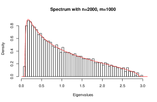
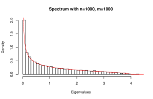
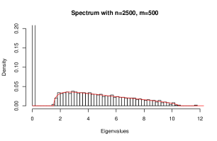
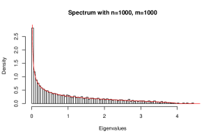
Figure 1: Example of residual spikes of $\hat{\hat{\Sigma}}_{X}^{-1/2}\hat{\Sigma}_{Y}\hat{\hat{\Sigma}}_{X}^{-1/2}$ when $\theta=10$ for the first three figures and $\theta_{1,2,3,4}=10,15,20,25$ for the last figure.

This paper studies these residual spikes by deriving the distribution of the extreme residual spikes under the null hypothesis. The philosophy is explained in Figure 2 with illustrations inspired by the i.i.d. normal case. All the eigenvalues lying in what we call the residual zone are potentially not indicative of real differences. However, when an eigenvalue is larger, we declare that this spike expresses a true difference.

Most of our plots feature the seemingly more natural matrix

$$\hat{\hat{\Sigma}}_{X}^{-1/2}\hat{\Sigma}_{Y}\hat{\hat{\Sigma}}_{X}^{-1/2}\,.$$

But, although this choice simplifies the study in terms of convergence in probability when the perturbation is of order $1$, this is no longer the case in more complex situations. In addition, the eigenvectors associated with the residual spikes are more accessible for the matrix in which all estimates are filtered.

Figure 2: Residual zone of $\hat{\hat{\Sigma}}_{X}^{-1/2}\hat{\Sigma}_{Y}\hat{\hat{\Sigma}}_{X}^{-1/2}$ and $\hat{\hat{\Sigma}}_{X}^{-1/2}\hat{\hat{\Sigma}}_{Y}\hat{\hat{\Sigma}}_{X}^{-1/2}$.

Let $\hat{\theta}_{X}$ and $\hat{\theta}_{Y}$ be isolated eigenvalues and construct the asymptotic unbiased estimators as in Equation (2.2)

$$\hat{\hat{\theta}}_{X}=1+\frac{1}{\frac{1}{m}\sum_{i=1}^{m}\frac{\hat{\lambda}_{W_{X},i}}{\hat{\theta}_{X}-\hat{\lambda}_{W_{X},i}}}\text{ and }\hat{\hat{\theta}}_{Y}=1+\frac{1}{\frac{1}{m}\sum_{i=1}^{m}\frac{\hat{\lambda}_{W_{Y},i}}{\hat{\theta}_{Y}-\hat{\lambda}_{W_{Y},i}}}\,.$$

Here $\hat{\lambda}_{W_{X},i}$ and $\hat{\lambda}_{W_{Y},i}$ are the eigenvalues of $W_{X}$ and $W_{Y}$, respectively. In practice we do of course not observe $W_{X}$ and $W_{Y}$, but a simple argument using Cauchy’s interlacing law shows that we can replace the previous estimators by

$$\hat{\hat{\theta}}_{X}=1+\frac{1}{\frac{1}{m-1}\sum_{i=2}^{m}\frac{\hat{\lambda}_{\hat{\Sigma}_{X},i}}{\hat{\theta}_{X}-\hat{\lambda}_{\hat{\Sigma}_{X},i}}}\text{ and }\hat{\hat{\theta}}_{Y}=1+\frac{1}{\frac{1}{m-1}\sum_{i=2}^{m}\frac{\hat{\lambda}_{\hat{\Sigma}_{Y},i}}{\hat{\theta}_{Y}-\hat{\lambda}_{\hat{\Sigma}_{Y},i}}},$$

where $\hat{\lambda}_{\hat{\Sigma}_{X},i}$ and $\hat{\lambda}_{\hat{\Sigma}_{Y},i}$ are the i^th ordered eigenvalue of $\hat{\Sigma}_{X}$ and $\hat{\Sigma}_{Y}$, respectively. The test statistic is then

$$\lambda_{\min}\left(\hat{\hat{\Sigma}}_{X}^{-1/2}\hat{\hat{\Sigma}}_{Y}\hat{\hat{\Sigma}}_{X}^{-1/2}\right)\text{ and }\lambda_{\max}\left(\hat{\hat{\Sigma}}_{X}^{-1/2}\hat{\hat{\Sigma}}_{Y}\hat{\hat{\Sigma}}_{X}^{-1/2}\right)\,,$$

where the filtered matrices are constructed as in (2.3). These two statistics provide a basis for a powerful and robust test for the equality of (detectable) perturbations $P_{X}$ and $P_{Y}$.

2.1 Null distribution

Obviously under $H_{0}$, $\lambda_{\max}\left(\hat{\hat{\Sigma}}_{X}^{-1/2}\hat{\hat{\Sigma}}_{Y}\hat{\hat{\Sigma}}_{X}^{-1/2}\right)$ is a function of $\theta=\theta_{X}=\theta_{Y}$. The suspected worst case occurs in the limit as $\theta\to\infty$ and it is this limit which will determine the critical values of the test. This can be checked by Criterion 2.3 which we discuss later. Let

$$\lambda_{\max}\left(\hat{\hat{\Sigma}}_{X}^{-1/2}\hat{\hat{\Sigma}}_{Y}\hat{\hat{\Sigma}}_{X}^{-1/2}\right)\leqslant\lim_{\theta\rightarrow\infty}\lambda_{\max}\left(\hat{\hat{\Sigma}}_{X}^{-1/2}\hat{\hat{\Sigma}}_{Y}\hat{\hat{\Sigma}}_{X}^{-1/2}\right)=V_{\max},$$

$$\lambda_{\min}\left(\hat{\hat{\Sigma}}_{X}^{-1/2}\hat{\hat{\Sigma}}_{Y}\hat{\hat{\Sigma}}_{X}^{-1/2}\right)\geqslant\lim_{\theta\rightarrow\infty}\lambda_{\min}\left(\hat{\hat{\Sigma}}_{X}^{-1/2}\hat{\hat{\Sigma}}_{Y}\hat{\hat{\Sigma}}_{X}^{-1/2}\right)=V_{\min}.$$

Because of our focus on the worst case scenario under $H_{0}$, we will investigate the asymptotics as $\frac{\theta}{\sqrt{m}}\rightarrow\infty$. Our test rejects the null hypothesis of equal populations if either $\mathit{P}\left(V_{\max}>\hat{\lambda}_{\max}\right)$ or $\mathit{P}\left(V_{\min}<\hat{\lambda}_{\min}\right)$ is small, where $\hat{\lambda}_{\max}$ and $\hat{\lambda}_{\min}$ are the observed extreme residual spikes.

In the investigation of the extremal eigenvalues under multiplicative perturbations, we make use of the following random variables

$$M_{s_{1},s_{2},X}(\rho_{X}) = \frac{1}{m}\sum_{i=1}^{m}\frac{\hat{\lambda}_{W_{X},i}^{s_{1}}}{\left(\rho_{X}-\hat{\lambda}_{W_{X},i}\right)^{2}},$$

$$M_{s_{1},s_{2},Y}(\rho_{Y}) = \frac{1}{m}\sum_{i=1}^{m}\frac{\hat{\lambda}_{W_{Y},i}^{s_{1}}}{\left(\rho_{Y}-\hat{\lambda}_{W_{Y},i}\right)^{2}},$$

$$M_{s_{1},s_{2}}(\rho_{X},\rho_{Y}) = \frac{M_{s_{1},s_{2},X}(\rho_{X})+M_{s_{1},s_{2},Y}(\rho_{Y})}{2}.$$

In particular, when $s_{2}=0$, we use $M_{s_{1},X}=M_{s_{1},0,X}$. When we only study one group, we use the simpler notation $M_{s_{1},s_{2}}(\rho)$ when no confusion is possible. Note that $M_{1,1,X}(\rho_{X})=\hat{T}_{W_{X}}(\rho_{X})$ is the empirical T-transform. Moreover, for an applied perspective, all these variables can be estimated by M_s_1,s_2,X(ρ_X)=^M_s_1,s_2,X(ρ_X)=1m-1 ∑_i=2^m ^λ^ΣX,is1(ρX-^λ^ΣX,i)2.

The following result describes the asymptotic behavior of the extreme eigenvalues and thus of $V_{\max}$ and $V_{\min}$. .

Theorem 2.1.

Suppose $W_{X},W_{Y}\in\mathbb{R}^{m\times m}$ are as described at the start of Section 2 and $P={\rm I}_{m}+(\theta-1)e_{1}e_{1}^{t}\in\mathbb{R}^{m\times m}$ with $\frac{\sqrt{m}}{\theta}=o(1)$ with regard to large $m$. Let

$$\hat{\Sigma}_{X}=P^{1/2}W_{X}P^{1/2}\text{ and }\hat{\Sigma}_{Y}=P^{1/2}W_{Y}P^{1/2}.$$

and $\hat{\hat{\Sigma}}_{X}$, $\hat{\hat{\Sigma}}_{Y}$ as described above (see, 2.1).

Then, conditional on the spectra $S_{W_{X}}=\left\{\hat{\lambda}_{W_{X},1},\hat{\lambda}_{W_{X},2},...,\hat{\lambda}_{W_{X},m}\right\}$ and $S_{W_{Y}}=\left\{\hat{\lambda}_{W_{Y},1},\hat{\lambda}_{W_{Y},2},...,\hat{\lambda}_{W_{Y},m}\right\}$ of $W_{X}$ and $W_{Y}$,

$$\left.\sqrt{m}\frac{\left(\lambda_{\max}\left(\hat{\hat{\Sigma}}_{X}^{-1/2}\hat{\hat{\Sigma}}_{Y}\hat{\hat{\Sigma}}_{X}^{-1/2}\right)-\lambda^{+}\right)}{\sigma^{+}}\right|S_{W_{X}},S_{W_{Y}}\sim\mathbf{N}(0,1)+o_{p}(1),$$

where

$$\lambda^{+}=\sqrt{M_{2}^{2}-1}+M_{2},\hskip 853.58267pt$$

$${\sigma^{+}}^{2}=\frac{1}{\left(M_{2,X}+M_{2,Y}-2\right)\left(M_{2,X}+M_{2,Y}+2\right)}\hskip 853.58267pt$$

$$\hskip 56.9055pt\Bigg{(}9M_{2,X}^{4}M_{2,Y}+4M_{2,X}^{3}M_{2,Y}^{2}+4M_{2,X}^{3}M_{2,Y}+2M_{2,X}^{3}M_{3,Y}-2M_{2,X}^{2}M_{2,Y}^{3}$$

$$\hskip 56.9055pt+4M_{2,X}^{2}M_{2,Y}^{2}-11M_{2,X}^{2}M_{2,Y}-8M_{3,X}M_{2,X}^{2}M_{2,Y}+2M_{2,X}^{2}M_{2,Y}M_{3,Y}$$

$$\hskip 56.9055pt-2M_{2,X}^{2}M_{3,Y}+M_{2,X}^{2}M_{4,Y}+4M_{2,X}M_{2,Y}^{3}+M_{2,X}M_{2,Y}^{2}+4M_{2,X}M_{2,Y}$$

$$\hskip 56.9055pt-4M_{3,X}M_{2,X}M_{2,Y}^{2}-4M_{3,X}M_{2,X}M_{2,Y}-2M_{2,X}M_{2,Y}^{2}M_{3,Y}-4M_{2,X}M_{2,Y}M_{3,Y}$$

$$\hskip 56.9055pt-6M_{2,X}M_{3,Y}+2M_{4,X}M_{2,X}M_{2,Y}+2M_{2,X}M_{2,Y}M_{4,Y}-2M_{3,X}M_{2,Y}^{2}$$

$$\hskip 56.9055pt+2M_{3,X}M_{2,Y}+M_{4,X}M_{2,Y}^{2}+4M_{2,X}^{5}+2M_{2,X}^{4}-4M_{3,X}M_{2,X}^{3}-13M_{2,X}^{3}$$

$$\hskip 56.9055pt-2M_{3,X}M_{2,X}^{2}+M_{4,X}M_{2,X}^{2}-2M_{2,X}^{2}+10M_{3,X}M_{2,X}+4M_{2,X}+4M_{3,X}$$

$$\hskip 56.9055pt-2M_{4,X}+M_{2,Y}^{5}+2M_{2,Y}^{4}-M_{2,Y}^{3}-2M_{2,Y}^{2}+4M_{2,Y}-2M_{2,Y}^{3}M_{3,Y}$$

$$\hskip 56.9055pt-2M_{2,Y}^{2}M_{3,Y}+2M_{2,Y}M_{3,Y}+4M_{3,Y}+M_{2,Y}^{2}M_{4,Y}-2M_{4,Y}-4\Bigg{)}$$

$$\hskip 35.56593pt+\frac{1}{\sqrt{\left(M_{2,X}+M_{2,Y}-2\right)\left(M_{2,X}+M_{2,Y}+2\right)}}$$

$$\hskip 56.9055pt\Bigg{(}5M_{2,X}^{3}M_{2,Y}-M_{2,X}^{2}M_{2,Y}^{2}+2M_{2,X}^{2}M_{2,Y}+2M_{2,X}^{2}M_{3,Y}-M_{2,X}M_{2,Y}^{3}$$

$$\hskip 56.9055pt+2M_{2,X}M_{2,Y}^{2}-4M_{2,X}M_{2,Y}-4M_{3,X}M_{2,X}M_{2,Y}-2M_{2,X}M_{3,Y}+M_{2,X}M_{4,Y}$$

$$\hskip 56.9055pt-2M_{3,X}M_{2,Y}+M_{4,X}M_{2,Y}+4M_{2,X}^{4}+2M_{2,X}^{3}-4M_{3,X}M_{2,X}^{2}-5M_{2,X}^{2}$$

$$\hskip 56.9055pt-2M_{3,X}M_{2,X}+M_{4,X}M_{2,X}+2M_{2,X}+2M_{3,X}+M_{2,Y}^{4}+2M_{2,Y}^{3}+M_{2,Y}^{2}$$

$$\hskip 56.9055pt+2M_{2,Y}-2M_{2,Y}^{2}M_{3,Y}-2M_{2,Y}M_{3,Y}-2M_{3,Y}+M_{2,Y}M_{4,Y}\Bigg{)},$$

$$M_{s,X}=\frac{1}{m}\sum_{i=1}^{m}\hat{\lambda}_{W_{X},i}^{s},\hskip 853.58267pt$$

$$M_{s,Y}=\frac{1}{m}\sum_{i=1}^{m}\hat{\lambda}_{W_{Y},i}^{s},$$

$$M_{s}=\frac{M_{s,X}+M_{s,Y}}{2}.$$

Moreover,

$$\left.\sqrt{m}\frac{\left(\lambda_{\min}\left(\hat{\hat{\Sigma}}_{X}^{-1/2}\hat{\hat{\Sigma}}_{Y}\hat{\hat{\Sigma}}_{X}^{-1/2}\right)-\lambda^{-}\right)}{\sigma^{-}}\right|S_{W_{X}},S_{W_{Y}}\sim\mathbf{N}(0,1)+o_{m}(1),$$

where

$$\lambda^{-}=-\sqrt{M_{2}^{2}-1}+M_{2},\hskip 853.58267pt$$

$${\sigma^{-}}^{2}=\left(\lambda^{-}\right)^{4}{\sigma^{+}}^{2}.$$

The error $o_{p}(1)$ in the approximation is with regard to large values of $m$.

Special case

If the spectra are Marcenko-Pastur distributed, then:

$$c=\frac{c_{X}+c_{Y}}{2},\text{ where }c_{X}=\frac{n_{X}}{m}\text{ and }c_{Y}=\frac{n_{Y}}{m},\hskip 853.58267pt$$

$$\lambda^{+}=c+\sqrt{c(c+2)}+1,$$

$${\sigma^{+}}^{2}=c_{X}^{3}+c_{X}^{2}c_{Y}+3c_{X}^{2}+4c_{X}c_{Y}-c_{X}+c_{Y}^{2}+c_{Y}$$

$$\hskip 56.9055pt+\frac{(8c_{X}+2c_{X}^{2}+\left(c_{X}^{3}+5c_{X}^{2}+c_{X}^{2}c_{Y}+4c_{X}c_{Y}+5c_{X}+3c_{Y}+c_{Y}^{2}\right)\sqrt{c(c+2)}}{c+2}.$$

If $c_{X}$ tends to $0$, then $\displaystyle{\sigma^{+}}^{2}$ $\displaystyle=$ $\displaystyle\Bigg{(}M_{2,Y}^{5}+2M_{2,Y}^{4}-2M_{3,Y}M_{2,Y}^{3}+M_{2,Y}^{3}-4M_{3,Y}M_{2,Y}^{2}+M_{4,Y}M_{2,Y}^{2}+2M_{2,Y}^{2}\hskip 853.58267pt$ $\displaystyle\hskip 28.45274pt+2M_{4,Y}M_{2,Y}+2M_{2,Y}-2M_{3,Y}-M_{4,Y}-2\Bigg{)}\Bigg{/}\Bigg{(}\left(M_{2,Y}-1\right)\left(M_{2,Y}+3\right)\Bigg{)}$ $\displaystyle+\Bigg{(}M_{2,Y}^{4}+M_{2,Y}^{3}-2M_{3,Y}M_{2,Y}^{2}+2M_{2,Y}^{2}-2M_{3,Y}M_{2,Y}+M_{4,Y}M_{2,Y}$ $\displaystyle\hskip 28.45274pt-2M_{3,Y}+M_{4,Y}\Bigg{)}\Bigg{/}\sqrt{\left(M_{2,Y}-1\right)\left(M_{2,Y}+3\right)}.$

(Proof in supplement material Mariétan and Morgenthaler (2019).)

2.2 Discussion and simulation

The above theorem gives the limiting distribution of $V_{\max}$ and $V_{\min}$. In this subsection, we first check the quality of the approximations in Theorem 2.1, then we investigate the worst case with regard to $\theta$.

2.2.1 Some simulations

Assume $\mathbf{X}\in\mathbb{R}^{m\times n_{X}}$ and $\mathbf{Y}\in\mathbb{R}^{m\times n_{Y}}$ with $\mathbf{X}=\left(X_{1},X_{2},...,X_{n_{X}}\right)$ and $\mathbf{Y}=\left(Y_{1},Y_{2},...,Y_{n_{Y}}\right)$. The components of the random vectors are independent and the covariance between the vectors is as follows:

$$X_{i}\sim\mathbf{N}_{m}\left(\vec{0},\sigma^{2}{\rm I}_{m}\right)\text{ with }X_{1}=\epsilon_{X,1}\text{ and }X_{i+1}=\rho X_{i}+\sqrt{1-\rho^{2}}\ \epsilon_{X,i+1},\text{ where }\epsilon_{X,i}\overset{i.i.d}{\sim}\mathbf{N}_{m}\left(\vec{0},\sigma^{2}{\rm I}_{m}\right),$$

$$Y_{i}\sim\mathbf{N}_{m}\left(\vec{0},\sigma^{2}{\rm I}_{m}\right)\text{ with }Y_{1}=\epsilon_{Y,1}\text{ and }Y_{i+1}=\rho Y_{i}+\sqrt{1-\rho^{2}}\ \epsilon_{Y,i+1},\text{ where }\epsilon_{Y,i}\overset{i.i.d}{\sim}\mathbf{N}_{m}\left(\vec{0},\sigma^{2}{\rm I}_{m}\right)$$

Let $P_{X}={\rm I}_{m}+(\theta_{X}-1)u_{X}u_{X}^{t}$ and $P_{Y}={\rm I}_{m}+(\theta_{Y}-1)u_{Y}u_{Y}^{t}$ be two perturbations in $\mathbb{R}^{m\times m}$. Then,

$$\mathbf{X}_{P}=P_{X}^{1/2}\mathbf{X}\text{ and }\mathbf{Y}_{P}=P_{Y}^{1/2}\mathbf{Y},$$

$$\hat{\Sigma}_{X}=\frac{\mathbf{X}_{P}^{t}\mathbf{X}_{P}}{n_{X}}\text{ and }\hat{\Sigma}_{Y}=\frac{\mathbf{Y}_{P}^{t}\mathbf{Y}_{P}}{n_{Y}}.$$

We assume a common and large value for $\theta$ and $P_{X}=P_{Y}$.

Distribution

Figure 1 presents empirical distributions of the extreme residual spikes in different scenarios together with the normal densities from our theorem.

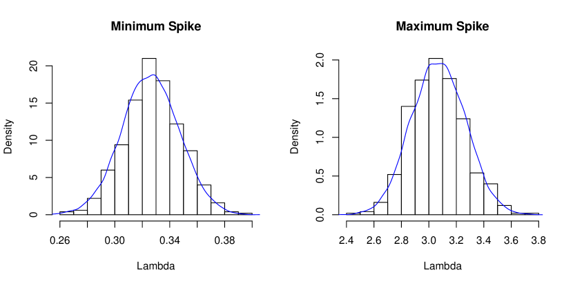
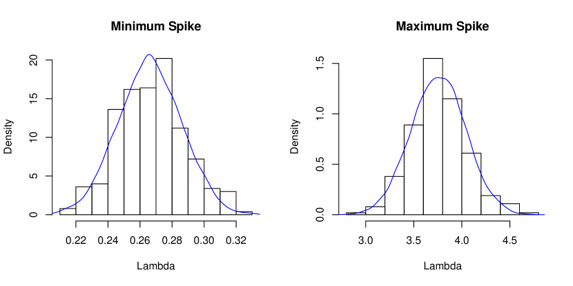
Scenario 1 $\rho=0.5$ $c_{X}=1/3$ $c_{Y}=1/2$ $m=300$ $n_{X}=900$ $n_{Y}=600$ $\theta=5^{\prime}000$.	Scenario 2 $\rho=0.$ $c_{X}=1$ $c_{Y}=1$ $m=300$ $n_{X}=300$ $n_{Y}=300$ $\theta=5^{\prime}000$.
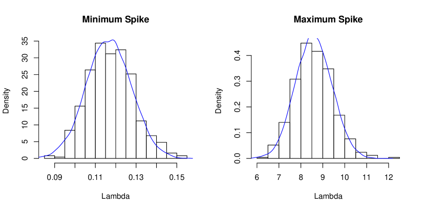
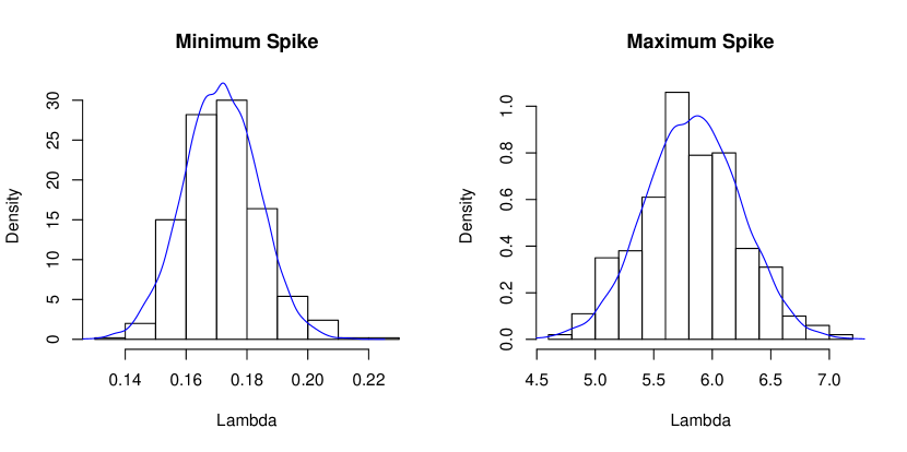
Scenario 3 $\rho=0.5$ $c_{X}=2$ $c_{Y}=2$ $m=600$ $n_{X}=300$ $n_{Y}=300$ $\theta=5^{\prime}000$.	Scenario 4 $\rho=0.$ $c_{X}=2$ $c_{Y}=2$ $m=600$ $n_{X}=300$ $n_{Y}=300$ $\theta=5^{\prime}000$.

Table 1: Empirical distributions of the residual spikes and the Gaussian densities from the theorem 2.1 (in blue).

Appendix A, Table 3 contains a comparison of the estimates of the mean and the variance with empirical ones in diverse situations. It is noticeable that in situations where $m$ is large compared to $n_{X}$ or $n_{Y}$, the asymptotic results are less accurate.

2.2.2 Increasing residual spike

In the four scenarios used in the simulations, we can estimate the expectation of the residual spike. Figure 3 shows that the expectations of the largest residual spikes are always strictly increasing as a function of $\theta$ and the expectations of the smallest residual spikes are always strictly decreasing. This is, however, not universally true. To address this issue, the following criterion can be used.

Definition 2.3.

Suppose $\hat{\Sigma}_{X}$ and $\hat{\Sigma}_{Y}$ are two independent random estimated covariance matrices of the form described at the start of Section 2. Let

where $S_{X}=\left\{\hat{\lambda}_{\hat{\Sigma}_{X},2},\hat{\lambda}_{\hat{\Sigma}_{X},3},...,\hat{\lambda}_{\hat{\Sigma}_{X},m}\right\}$ and $S_{Y}=\left\{\hat{\lambda}_{\hat{\Sigma}_{Y},2},\hat{\lambda}_{\hat{\Sigma}_{Y},3},...,\hat{\lambda}_{\hat{\Sigma}_{Y},m}\right\}$ and

We say that the criterion is satisfied, if this estimate of the expectation of the residual spike is a monotone increasing function of $\theta$.

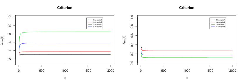
Figure 3: Plot of the criterion in the four scenarios used in the simulation.

Remark 2.1.

The above estimate of the expectation of a residual spike fails when $\theta$ is large compared to $m$ and we should then use an asymptotic estimator of $\alpha$ based on:

Using this approximation, the estimated curve of the equation (2.5) makes an error of $O_{p}\left(1/\theta^{2}\right)$.

3 Further Results

The proof of the main distributional result (Theorem 2.1) is based on three results and a lemma that are worthwhile on their own right and will be presented and discussed in this section. Future papers will also use this result for extensions.

3.1 Unit invariant vector statistic

Theorem 3.1.

Let $W$ be a random matrix with spectrum $S_{W}=\left\{\hat{\lambda}_{W,1},\hat{\lambda}_{W,2},...,\hat{\lambda}_{W,m}\right\}$ and trace equal to $m$. We denote by $u_{p_{1}}$ and $u_{p_{2}}$, two orthonormal invariant random vectors of size $m$ and independent of the eigenvalues of $W$. We set

$$\vec{B}_{m}\left(\rho,\vec{s},\vec{r},\vec{p}\right)=\sqrt{m}\left(\begin{pmatrix}\sum_{i=1}^{m}\frac{\hat{\lambda}_{W,i}^{s_{1}}}{\left(\rho-\hat{\lambda}_{W,i}\right)^{s_{2}}}{u}_{p_{1},i}{u}_{p_{2},i}\\ \sum_{i=1}^{m}\frac{\hat{\lambda}_{W,i}^{r_{1}}}{\left(\rho-\hat{\lambda}_{W,i}\right)^{r_{2}}}{u}_{p_{1},i}{u}_{p_{2},i}\end{pmatrix}-\begin{pmatrix}M_{s_{1},s_{2}}\\ M_{r_{1},r_{2}}\end{pmatrix}\mathbf{1}_{p_{1}=p_{2}}\right),$$

where $\vec{s}=\left(s_{1},s_{2}\right)$, $\vec{r}=\left(r_{1},r_{2}\right)$ and $\vec{p}=\left(p_{1},p_{2}\right)$ with indices $1\leqslant p_{1}\leqslant p_{2}\leqslant m$ and $s_{1},s_{2},r_{1},r_{2}\in\mathbf{N}$. If $p=p_{1}=p_{2}$,

where $M_{s,r}=M_{s,r}(\rho)=\frac{1}{m}\sum_{i=1}^{m}\frac{\hat{\lambda}_{W,i}^{s}}{\left(\rho-\hat{\lambda}_{W,i}\right)^{r}}$. Moreover, for $p_{1}\neq p_{2}$,

In particular, with the notation $M_{s,0}=M_{s}=\frac{1}{m}\sum_{i=1}^{m}\hat{\lambda}_{W,i}^{s}$,

and

Finally if we look at $K$ bivariate normal random variables :

where $\vec{p}_{i}\neq\vec{p}_{j}$ if $i\neq j$. Then, conditioning on the spectrum $S_{W}$, $\mathbf{{B}}_{m}\left(\vec{\rho},\mathbf{{s}},\mathbf{{r}},\mathbf{{p}}\right)$ tends to a multivariate Normal. Moreover, all the bivariate elements $\vec{B}_{m}\left(\rho_{i},\vec{s}_{i},\vec{r}_{i},\vec{p}_{i}\right)$ are asymptotically independent.

Remark 3.1.1.

1. The trace of $W$ equal to $m$ can easily be obtained by rescaling the matrix.

2. Although the condition of independence between eigenvectors and eigenvalues of $W$ appears to be restrictive, it is an automatic consequence if the eigenvectors are Haar distributed.

3. If $W$ is a rescaled standard Wishart, then

   where $\hat{u}_{1},\hat{u}_{2},...,\hat{u}_{m}$ are the eigenvectors of $W$.

(Proof in supplement material Mariétan and Morgenthaler (2019).)

3.2 Characterisation and convergence of eigenvalues and angles

In this section, we study the convergence of the random variable $\hat{\hat{\theta}}_{X}$ and the angle between the eigenvectors. The proof for the parts $2.a$ and $2.b$ are given in Benaych-Georges and Rao (2009), which also provides the main idea for the proof. We only show convergence results for perturbations of order $k=1$, although we express eigenvectors and eigenvalues of a matrix $P^{1/2}WP^{1/2}$ as a function of the eigenstructure of $W$ in general and $W$ can already be perturbed.

Theorem 3.2.

In this theorem, $P={\rm I}_{m}+(\theta-1)uu^{t}$ is a finite perturbation of order $1$.

1. Suppose $W$ is a symmetric matrix with eigenvalues $\hat{\lambda}_{W,i}\geqslant 0$ and eigenvectors $\hat{u}_{W,i}$ for $i=1,2,...,m$. The perturbation of $W$ by $P$ leads to $\hat{\Sigma}=P^{1/2}WP^{1/2}$.

For $i=1,2,...,m$, we define $\tilde{u}_{\hat{\Sigma},i}$ and $\hat{\lambda}_{\hat{\Sigma},i}$ such that W P ~u_^Σ,i = ^λ_^Σ,i ~u_^Σ,i, and the usual $\hat{u}_{\hat{\Sigma},i}$ such that if $\hat{\Sigma}=P^{1/2}WP^{1/2}$, then ^Σ ^u_^Σ,i = P^1/2 W P^1/2 ^u_^Σ,i = ^λ_^Σ,i ^u_^Σ,i. Under these conditions, the following results hold:

• The eigenvalues $\hat{\lambda}_{\hat{\Sigma},s}$ are such that for $s=1,2,...,m$,

  $$\sum_{i=1}^{m}\frac{\hat{\lambda}_{W,i}}{\hat{\lambda}_{\hat{\Sigma},s}-\hat{\lambda}_{W,i}}\left\langle\hat{u}_{W,i},u\right\rangle^{2}=\frac{1}{\theta-1}.$$

• The eigenvectors $\tilde{u}_{\hat{\Sigma},s}$ are such that

  $$\left\langle\tilde{u}_{\hat{\Sigma},s},v\right\rangle^{2}=\frac{\left(\sum_{i=1}^{m}\frac{\hat{\lambda}_{W,i}}{\hat{\lambda}_{\hat{\Sigma},s}-\hat{\lambda}_{W,i}}\left\langle\hat{u}_{W,i},v\right\rangle\left\langle\hat{u}_{W,i},u\right\rangle\right)^{2}}{\sum_{i=1}^{m}\frac{\hat{\lambda}_{W,i}^{2}}{(\hat{\lambda}_{\hat{\Sigma},s}-\hat{\lambda}_{W,i})^{2}}\left\langle\hat{u}_{W,i},u\right\rangle^{2}}.$$

  In particular if $v=u$,

  $$\left\langle\tilde{u}_{\hat{\Sigma},s},u\right\rangle^{2} = \frac{1}{\left(\theta-1\right)^{2}\left(\sum_{i=1}^{m}\frac{\hat{\lambda}_{W,i}^{2}}{(\hat{\lambda}_{\hat{\Sigma},s}-\hat{\lambda}_{W,i})^{2}}\left\langle\hat{u}_{W,i},u\right\rangle^{2}\right)}.$$

  Moreover,

  $$\hat{u}_{\hat{\Sigma},s}=\frac{P^{1/2}\tilde{u}_{\hat{\Sigma},s}}{\sqrt{1+\left(\theta-1\right)\left\langle\tilde{u}_{\hat{\Sigma},s},u\right\rangle^{2}}}.$$

  Therefore, for $u$ and $v$ such that $\left\langle v,u\right\rangle=0$,

  $$\left\langle\hat{u}_{\hat{\Sigma},s},u\right\rangle^{2} = \frac{\theta\left\langle\tilde{u}_{\hat{\Sigma},s},u\right\rangle^{2}}{1+\left(\theta-1\right)\left\langle\tilde{u}_{\hat{\Sigma},s},u\right\rangle^{2}}=-\frac{\theta}{(\theta-1)^{2}\hat{\lambda}_{\hat{\Sigma},s}T_{W,u}^{\prime}(\hat{\lambda}_{\hat{\Sigma},s})},$$

  $$\left\langle\hat{u}_{\hat{\Sigma},s},v\right\rangle^{2} = \frac{\left\langle\tilde{u}_{\hat{\Sigma},s},u\right\rangle^{2}}{1+\left(\theta-1\right)\left\langle\tilde{u}_{\hat{\Sigma},s},u\right\rangle^{2}},$$

  where $T_{W,u}(z)=\sum_{i=1}^{m}\frac{\hat{\lambda}_{W,i}}{z-\hat{\lambda}_{W,i}}\left\langle\hat{u}_{W,i},u\right\rangle^{2}$ is a weighted empirical T-transform.

Suppose that $W_{X}$, $W_{Y}$ and $P=P_{X}=P_{Y}$ satisfy the conditions described at the start of Section 2. Moreover, suppose that $\theta$ is large enough to create detectable spikes, $\left(\hat{\theta}_{X},\hat{u}_{X}\right)$ and $\left(\hat{\theta}_{Y},\hat{u}_{Y}\right)$, in the matrices $\hat{\Sigma}_{X}=P^{1/2}W_{X}P^{1/2}$ and $\hat{\Sigma}_{Y}=P^{1/2}W_{Y}P^{1/2}$. Then,

$$a) \hat{\hat{\theta}}_{X},\hat{\hat{\theta}}_{Y}\underset{n,m\rightarrow\infty}{\overset{P}{\longrightarrow}}\theta,$$

$$b) \left\langle\hat{u}_{X},u\right\rangle-\alpha_{X},\left\langle\hat{u}_{Y},u\right\rangle-\alpha_{Y}\underset{n,m\rightarrow\infty}{\overset{P}{\longrightarrow}}0,$$

$$c) \left\langle\hat{u}_{X},\hat{u}_{Y}\right\rangle-\alpha_{X}\alpha_{Y}\underset{n,m\rightarrow\infty}{\overset{P}{\longrightarrow}}0,$$

where

$$\hat{\theta}_{X}\underset{n,m\rightarrow\infty}{\overset{P}{\longrightarrow}}\rho_{X},$$

$$\hat{\hat{\theta}}_{X}=1+\frac{1}{\hat{T}_{\hat{\Sigma}_{X}}\left(\hat{\theta}_{X}\right)}=1+\frac{m}{\sum_{i=k+1}^{m}\frac{\hat{\lambda}_{\hat{\Sigma}_{X},i}}{\hat{\theta}_{X}-\hat{\lambda}_{\hat{\Sigma}_{X},i}}},$$

$$\alpha_{X}^{2}=-\frac{\theta}{(\theta-1)^{2}\rho_{X}\hat{T}_{W_{X}}^{\prime}(\rho_{X})},$$

$$\alpha_{Y}^{2}=-\frac{\theta}{(\theta-1)^{2}\rho_{Y}\hat{T}_{W_{Y}}^{\prime}(\rho_{Y})},$$

$$\hat{\lambda}_{\hat{\Sigma}_{X},i}\text{ and }\hat{\lambda}_{\hat{\Sigma}_{Y},i}\text{ are the eigenvalues of respectively }\hat{\Sigma}_{X}\text{ and }\hat{\Sigma}_{Y}.$$

Note that $\hat{T}_{W_{X}}(z)=\frac{1}{m}\sum_{i=1}^{m}\frac{\hat{\lambda}_{W_{X},i}}{z-\hat{\lambda}_{W_{X},i}}$ and $\hat{T}_{\hat{\Sigma}_{X}}(z)=\frac{1}{m}\sum_{i=k+1}^{m}\frac{\hat{\lambda}_{\hat{\Sigma}_{X},i}}{z-\hat{\lambda}_{\hat{\Sigma}_{X},i}}$ are empirical T-transform and its estimation.

Remark 3.2.1.

If the spectra of $W_{X}$ and $W_{Y}$ are Wishart random matrices of size $m$ and degree of freedom $n_{X}$, $n_{Y}$ respectively, then by setting $c_{X}=\frac{m}{n_{X}}$ and $c_{Y}=\frac{m}{n_{Y}}$

$$\alpha_{X}^{2}=\frac{1-\frac{c_{X}}{(\theta-1)^{2}}}{1+\frac{c_{X}}{\theta-1}},$$

$$\hat{\hat{\theta}}_{X}\text{ is such that }\hat{\theta}_{X}=\hat{\hat{\theta}}_{X}\left(1+\frac{c_{X}}{\hat{\hat{\theta}}_{X}-1}\right),\text{ and}$$

$$\underset{m\rightarrow\infty}{\lim}\hat{\theta}_{X}=\theta\left(1+\frac{c_{X}}{\theta-1}\right).$$

(Proof in supplement material Mariétan and Morgenthaler (2019).)

The second part of Theorem 3.2 is very surprising! We already knew that the eigenvectors are not consistent. We show in the proof that the dot product of $\hat{u}_{X}$ and $\hat{u}_{Y}$ is smaller than that of $\hat{u}_{X}$ and $u$ and that of $\hat{u}_{Y}$ and $u$. Among the consequences of this theorem is the fact that there is always an asymptotic bias between two eigenvectors, even if they are equal.

3.3 Asymptotic distribution of the eigenvalues and the angle

Suppose that you observe a perturbation of order $k=1$ applied to two random matrices $W_{X}\in\mathbb{R}^{m\times m}$ and $W_{Y}\in\mathbb{R}^{m\times m}$. We investigate the distribution of $\hat{\hat{\theta}}_{X}$, $\hat{\hat{\theta}}_{Y}$, $\left\langle\hat{u}_{X},u\right\rangle^{2}$ and $\left\langle\hat{u}_{X},\hat{u}_{Y}\right\rangle^{2}$.

Theorem 3.3.

Suppose $W_{X}$ and $W_{Y}$ satisfy the conditions described at the start of Section 2 with $P=P_{X}=P_{Y}={\rm I}_{m}+(\theta-1)uu^{t}$, a detectable perturbation of order $k=1$. Moreover, we assume $S_{W_{X}}=\left\{\hat{\lambda}_{W_{X},1},\hat{\lambda}_{W_{X},2},...,\hat{\lambda}_{W_{X},m}\right\}$ and $S_{W_{Y}}=\left\{\hat{\lambda}_{W_{Y},1},\hat{\lambda}_{W_{Y},2},...,\hat{\lambda}_{W_{Y},m}\right\}$, the eigenvalues of $W_{X}$ and $W_{Y}$ as known. We defined

$$\hat{\Sigma}_{X} = P^{1/2}W_{X}P^{1/2},$$

$$\hat{\Sigma}_{Y} = P^{1/2}W_{Y}P^{1/2}.$$

We construct the unbiased estimators of $\theta$, $\hat{\hat{\theta}}_{X}$ and $\hat{\hat{\theta}}_{Y}$ via the relationship

$$\frac{1}{\hat{\hat{\theta}}_{X}-1}=\frac{1}{m}\sum_{i=1}^{m}\frac{\hat{\lambda}_{W_{X},i}}{\hat{\theta}_{X}-\hat{\lambda}_{W_{X},i}}\ \text{ and }\frac{1}{\hat{\hat{\theta}}_{Y}-1}=\frac{1}{m}\sum_{i=1}^{m}\frac{\hat{\lambda}_{W_{Y},i}}{\hat{\theta}_{Y}-\hat{\lambda}_{W_{Y},i}}\,,$$

where $\hat{\theta}_{X}=\hat{\lambda}_{\hat{\Sigma}_{X},1}$ and $\hat{\theta}_{Y}=\hat{\lambda}_{\hat{\Sigma}_{Y},1}$ are the largest eigenvalues of $\hat{\Sigma}_{X}$ and $\hat{\Sigma}_{Y}$ corresponding to the eigenvectors $\hat{u}_{X}=\hat{u}_{\hat{\Sigma}_{X},1}$ and $\hat{u}_{Y}=\hat{u}_{\hat{\Sigma}_{Y},1}$.

1. If $\frac{\theta}{\sqrt{m}}\rightarrow 0$, we define

   where we assume

   $$\rho_{X}=\operatorname{E}\left[\hat{\theta}_{X}\right]+o\left(\frac{\theta}{\sqrt{m}}\right), \rho_{Y}=\operatorname{E}\left[\hat{\theta}_{Y}\right]+o\left(\frac{\theta}{\sqrt{m}}\right)$$

   and a convergence rate of $(\hat{\theta}_{X},\hat{\theta}_{Y})$ to $\left(\rho_{X},\rho_{Y}\right)$ in $O_{p}\left(1/\sqrt{m}\right)$. Then

   where

$$\alpha_{X}^{2}=\frac{\theta}{(\theta-1)^{2}}\frac{1}{\rho_{X}M_{1,2,X}},$$

$$\alpha_{X,Y}^{2}=\frac{\theta^{2}}{(\theta-1)^{4}}\frac{1}{\rho_{X}\rho_{Y}M_{1,2,X}M_{1,2,Y}},$$

$$\sigma_{\theta,X}^{2}=\frac{2\left(M_{2,2,X}-M_{1,1,X}^{2}\right)}{M_{1,1,X}^{4}},\hskip 853.58267pt$$

$$\sigma_{\alpha^{2},X}^{2}=\frac{2\theta^{2}}{\left((\theta-1)\rho_{X}M_{1,2,X}\right)^{4}}\left(\rho_{X}^{2}\left(M_{2,4,X}-M_{1,2,X}^{2}\right)+\left(2\rho_{X}\frac{M_{1,3,X}}{M_{1,2,X}}-1\right)^{2}\left(M_{2,2,X}-M_{1,1,X}^{2}\right)\right.$$

$$\hskip 56.9055pt\left.-2\rho_{X}\left(2\rho_{X}\frac{M_{1,3,X}}{M_{1,2,X}}-1\right)\left(M_{2,3,X}-\frac{M_{1,1,X}}{M_{1,2,X}}\right)\right),$$

$$\sigma_{\theta,\alpha^{2},X}=\frac{2\theta}{M_{1,1,X}^{2}M_{1,2,X}^{3}\rho_{X}^{2}(-1+\theta)^{2}}\bigg{(}M_{1,1,X}M_{1,2,X}^{2}\rho_{X}+2M_{1,3,X}M_{2,2,X}\rho_{X}$$

$$\hskip 56.9055pt+M_{1,1,X}^{2}(M_{1,2,X}-2M_{1,3,X}\rho_{X})-M_{1,2,X}(M_{2,2,X}+M_{2,3,X}\rho_{X})\bigg{)},$$

$$\sigma_{\alpha^{2},X,Y}^{2}=\sigma_{\alpha^{2},X}^{2}\alpha_{Y}^{4}+\sigma_{\alpha^{2},Y}^{2}\alpha_{X}^{4}+4\alpha_{X,Y}^{2}(1-\alpha_{X}^{2})(1-\alpha_{X}^{2}).\hskip 853.58267pt$$

If $\frac{\theta}{\sqrt{m}}\rightarrow\infty$, then we can simplify the formulas. We define

$$M_{r,X}=\frac{1}{m}\sum_{i=1}^{m}\hat{\lambda}_{W_{X},i}^{r} M_{r,Y}=\frac{1}{m}\sum_{i=1}^{m}\hat{\lambda}_{W_{Y},i}^{r}.$$ and

Using this notation, $\displaystyle\left.\begin{pmatrix}\hat{\hat{\theta}}_{X}\\ \left\langle\hat{u}_{X},u\right\rangle^{2}\end{pmatrix}\right|S_{W_{X}}\sim\mathbf{N}\left(\begin{pmatrix}\theta+O_{p}\left(1\right)\\ 1+\frac{1-M_{2,X}}{\theta}+O_{p}\left(\frac{1}{\theta^{2}}\right)\end{pmatrix},\right.$ $\displaystyle\hskip 65.44142pt\left.\frac{1}{m}\begin{pmatrix}2\theta^{2}\left(1-M_{2,X}\right)&2\left(2M_{2,X}^{2}-M_{2,X}-M_{3,X}\right)\\ 2\left(2M_{2,X}^{2}-M_{2,X}-M_{3,X}\right)&\frac{2}{\theta^{2}}\left(4M_{2,X}^{3}-M_{2,X}^{2}-4M_{2,X}M_{3,X}+M_{4,X}\right)\end{pmatrix}\right)+\begin{pmatrix}o_{p}\left(\frac{\theta}{\sqrt{m}}\right)\\ o_{p}\left(\frac{1}{\theta\sqrt{m}}\right)\end{pmatrix},$ $\displaystyle\left.\begin{pmatrix}\hat{\hat{\theta}}_{X}\\ \hat{\hat{\theta}}_{Y}\\ \left\langle\hat{u}_{X},\hat{u}_{Y}\right\rangle^{2}\end{pmatrix}\right|S_{W_{X}},S_{W_{Y}}\sim\mathbf{N}\left(\begin{pmatrix}\theta+O_{p}\left(1\right)\\ \theta+O_{p}\left(1\right)\\ 1+\frac{2-M_{2,X}-M_{2,Y}}{\theta}+O_{p}\left(\frac{1}{\theta^{2}}\right)\end{pmatrix},\right.$ $\displaystyle\hskip 51.21504pt\left.\frac{1}{m}\begin{pmatrix}2\theta^{2}\left(1-M_{2,X}\right)&0&2\left(2M_{2,X}^{2}-M_{2,X}-M_{3,X}\right)\\ 0&2\theta^{2}\left(1-M_{2,Y}\right)&2\left(2M_{2,Y}^{2}-M_{2,Y}-M_{3,Y}\right)\\ 2\left(2M_{2,X}^{2}-M_{2,X}-M_{3,X}\right)&2\left(2M_{2,Y}^{2}-M_{2,Y}-M_{3,Y}\right)&\frac{S}{\theta^{2}}\end{pmatrix}\right)+\begin{pmatrix}o_{p}\left(\frac{\theta}{\sqrt{m}}\right)\\ o_{p}\left(\frac{\theta}{\sqrt{m}}\right)\\ o_{p}\left(\frac{1}{\theta\sqrt{m}}\right)\end{pmatrix},$ $\displaystyle S=2\left(4M_{2,X}^{3}-M_{2,X}^{2}-4M_{2,X}M_{3,X}+M_{4,X}\right)+2\left(4M_{2,Y}^{3}-M_{2,Y}^{2}-4M_{2,Y}M_{3,Y}+M_{4,Y}\right)+4(M_{2,Y}-1)(M_{2,X}-1).$

Moreover, the asymptotic distributions of $\hat{\theta}_{X}$ and $\hat{\hat{\theta}}_{X}$ are the same.

If $\frac{\theta}{\sqrt{m}}\rightarrow d$, a finite constant, then a mixture of the two first scenarios describes the first two moments of the joint distribution. The formula of the second moment is asymptotically the same as the variance formula when $\frac{\theta}{\sqrt{m}}\rightarrow\infty$. The formula of the first moment is asymptotically the same as the expectation formula when $\frac{\theta}{\sqrt{m}}\rightarrow 0$.

The random variables can be expressed as functions of invariant unit random statistics of the form:

$$\overset{u}{M}_{r,s,X}(\rho) = \sum_{i=1}^{m}\frac{\hat{\lambda}^{r}_{W_{X},i}}{\left(\rho-\hat{\lambda}_{W_{X},i}\right)^{s}}\left\langle\hat{u}_{W_{X},i},u\right\rangle^{2}.$$

(Assuming a canonical perturbation leads to a simpler formula) Knowing $S_{W_{X}}$ and $S_{W_{Y}}$ we have

• Exact distributions:

  $$\hat{\theta}_{X}\left|\frac{1}{\theta-1}=\overset{u}{M}_{1,1,X}\left(\hat{\theta}_{X}\right)\right.,$$

  $$\left\langle\hat{u}_{X},e_{1}\right\rangle^{2}=\frac{\theta}{(\theta-1)^{2}}\frac{1}{\hat{\theta}_{X}\overset{u}{M}_{1,2,X}\left(\hat{\theta}_{X}\right)}.$$

  Moreover,

  $$\left\langle\hat{u}_{X},\hat{u}_{Y}\right\rangle = \left\langle\hat{u}_{X},e_{1}\right\rangle\left\langle\hat{u}_{Y},e_{1}\right\rangle+\sqrt{1-\left\langle\hat{u}_{X},e_{1}\right\rangle^{2}}\sqrt{1-\left\langle\hat{u}_{Y},e_{1}\right\rangle^{2}}Z,$$

  $$\sum_{i=2}^{m}\hat{u}_{X,1}\hat{u}_{Y,1} = \sqrt{1-\left\langle\hat{u}_{X},e_{1}\right\rangle^{2}}\sqrt{1-\left\langle\hat{u}_{Y},e_{1}\right\rangle^{2}}Z,$$

  $$Z \sim \mathbf{N}\left(0,\frac{1}{m}\right)+O_{p}\left(\frac{1}{m}\right),$$

  where $Z$ is independent of $\left\langle\hat{u}_{X},e_{1}\right\rangle$, $\left\langle\hat{u}_{Y},e_{1}\right\rangle$, $\hat{\theta}_{X}$ and $\hat{\theta}_{Y}$. In order to get the exact distribution, we should replace $Z$ by $\sum_{i=1}^{m-1}v_{i}\tilde{v}_{i}$ where $v_{i}$ and $\tilde{v}_{i}$ are independent unit invariant random vectors.

• Approximations:

  $$\hat{\theta}_{X} = \rho+\frac{\left(\overset{u}{M}_{1,1,X}\left(\rho\right)-{M}_{1,1,X}(\rho)\right)}{M_{1,2,X}\left(\rho\right)}+O_{p}\left(\frac{\theta}{m}\right)$$

  $$= \theta\overset{u}{M}_{1,X}+O_{p}\left(1\right),$$

  $$\hat{\hat{\theta}}_{X} = \theta+(\theta-1)^{2}\left(\overset{u}{M}_{1,1,X}\left(\rho\right)-{M}_{1,1,X}(\rho_{X})\right)+O_{p}\left(\frac{\theta}{m}\right).$$

  We provide three methods of estimation of the angle in order to estimate it for all $\theta$.

Finally, the double angle is such that $\displaystyle\left\langle\hat{u}_{X},\hat{u}_{Y}\right\rangle=\left\langle\hat{u}_{X},e_{1}\right\rangle\left\langle\hat{u}_{Y},e_{1}\right\rangle+\frac{\sqrt{M_{2,X}-1}\sqrt{M_{2,Y}-1}}{\theta}Z+O_{p}\left(\frac{1}{\theta^{2}\sqrt{m}}\right).$

Remark 3.3.1.

If the spectra of $W_{X}$ and $W_{Y}$ are rescaled Wishart matrices of size $m$ with $n$ degree of freedom. By setting $c=\frac{m}{n}$

$$\begin{pmatrix}\hat{\hat{\theta}}_{X}\\ \left\langle\hat{u}_{X},u_{0}\right\rangle^{2}\end{pmatrix}\overset{Asy}{\sim}\mathbf{N}\left(\begin{pmatrix}\theta\\ \frac{1-\frac{c}{(\theta-1)^{2}}}{1+\frac{c}{\theta-1}}\end{pmatrix},\frac{1}{m}\left(\begin{array}[]{cc}-\frac{2c(\theta-1)^{2}\theta^{2}}{c-(\theta-1)^{2}}&-\frac{2c^{2}(\theta-1)\theta^{3}}{\left(c-(\theta-1)^{2}\right)(c+\theta-1)^{2}}\\ -\frac{2c^{2}(\theta-1)\theta^{3}}{\left(c-(\theta-1)^{2}\right)(c+\theta-1)^{2}}&-\frac{2c^{2}\theta^{2}\left(c^{2}+(\theta(\theta+2)-2)c+(\theta-1)^{2}\right)}{\left(c-(\theta-1)^{2}\right)(c+\theta-1)^{4}}\\ \end{array}\right)\right)$$

and $\displaystyle\begin{pmatrix}\hat{\hat{\theta}}_{X}\\ \hat{\hat{\theta}}_{Y}\\ \left\langle\hat{u}_{X},\hat{u}_{Y}\right\rangle^{2}\end{pmatrix}\overset{Asy}{\sim}\mathbf{N}\left(\begin{pmatrix}\theta\\ \theta\\ \left(\frac{1-\frac{c}{(\theta-1)^{2}}}{1+\frac{c}{\theta-1}}\right)^{2}\end{pmatrix}\right.,$ $\displaystyle\hskip 42.67912pt\left.\frac{1}{m}\begin{pmatrix}-\frac{2c(\theta-1)^{2}\theta^{2}}{c-(\theta-1)^{2}}&0&-\frac{2c^{2}(\theta-1)\theta^{3}}{\left(c-(\theta-1)^{2}\right)(c+\theta-1)^{2}}\\ 0&-\frac{2c(\theta-1)^{2}\theta^{2}}{c-(\theta-1)^{2}}&-\frac{2c^{2}(\theta-1)\theta^{3}}{\left(c-(\theta-1)^{2}\right)(c+\theta-1)^{2}}\\ -\frac{2c^{2}(\theta-1)\theta^{3}}{\left(c-(\theta-1)^{2}\right)(c+\theta-1)^{2}}&-\frac{2c^{2}(\theta-1)\theta^{3}}{\left(c-(\theta-1)^{2}\right)(c+\theta-1)^{2}}&\frac{4c^{2}\theta^{2}\left(c-(\theta-1)^{2}\right)^{2}\left(c^{3}+4c^{2}(\theta-1)+c(\theta-1)(\theta(\theta+5)-5)+2(\theta-1)^{3}\right)}{(\theta-1)^{4}(c+\theta-1)^{7}}\end{pmatrix}\right).$

If $\theta$ tends to infinity, then (^^θX⟨^uX,u ⟩2) Asy∼ N((θ1-c(θ-1)21+cθ-1) , 1m(2 c θ22c22c22 c2(c+1)θ2)). Moreover, (^^θX^^θY⟨^uX,^uX⟩2) Asy∼ N((θθ1-c(θ-1)21+cθ-1), 1m(2c θ20 2c20 2c θ22c22c22c24 c2(c+2)θ2) ).

(Proof in supplement material Mariétan and Morgenthaler (2019).)

3.4 Residual spike as a function of the statistics

Finally we present a simple result of linear algebra that express the residual spike as a function of the statistics.

Lemma 3.1.

Suppose

The eigenvalues of $D$ are $1$ and

where $\alpha^{2}=\left\langle u_{X},u_{Y}\right\rangle^{2}$. Moreover, if

The eigenvalues of $D_{2}$ are $1$ and

where $\alpha^{2}=\left\langle u_{X},u_{Y}\right\rangle^{2}$. (Proof in supplement material Mariétan and Morgenthaler (2019).)

4 Comparison with existing tests

In the classical multivariate theory, Anderson (1958) proposes a log-ratio test for the equality of two covariance matrices. Suppose

$$X_{1},X_{2},...,X_{n_{X}}\overset{i.i.d.}{\sim}\mathbf{N}_{m}(0,\Sigma_{X}),$$

$$Y_{1},Y_{2},...,Y_{n_{Y}}\overset{i.i.d.}{\sim}\mathbf{N}_{m}(0,\Sigma_{Y}).$$

We want to test

$${\rm H}_{0}:\Sigma_{X}=\Sigma_{Y},$$

$${\rm H}_{1}:\Sigma_{X}\neq\Sigma_{Y},$$

The log-likelihood ratio test look at the statistic

$$T_{1}=n_{X}\log\left(\left|\frac{n_{X}}{n_{X}+n_{Y}}{\rm I}_{m}+\frac{n_{Y}}{n_{X}+n_{Y}}\hat{\Sigma}_{X}^{-1/2}\hat{\Sigma}_{Y}\hat{\Sigma}_{X}^{-1/2}\right|\right).$$

Under ${\rm H}_{0}$ and if $m$ is finite, $T_{1}\overset{D}{\rightarrow}\chi^{2}_{\frac{p(p-1)}{2}}$. Some other interesting tests propose to observe the determinant and the trace of $\hat{\Sigma}_{X}^{-1/2}\hat{\Sigma}_{Y}\hat{\Sigma}_{X}^{-1/2}$. In this section we show that any test statistics using $T_{2}=\log\left|\hat{\Sigma}_{X}^{-1/2}\hat{\Sigma}_{Y}\hat{\Sigma}_{X}^{-1/2}\right|$ or $T_{3}={{\rm Trace}}\left(\hat{\Sigma}_{X}^{-1/2}\hat{\Sigma}_{Y}\hat{\Sigma}_{X}^{-1/2}\right)$ have difficulties to test

$${\rm H}_{0}:P_{X}=P_{Y},$$

$${\rm H}_{1}:P_{X}\neq P_{Y},$$

when $P_{X}$ and $P_{Y}$ are finite perturbations. We compare the performance of these tests with our procedure $T$ defined in Section 2.1 in the table 2.

1. When $T=\left(\lambda_{\min}\left(\hat{\hat{\Sigma}}_{X}^{-1/2}\hat{\hat{\Sigma}}_{Y}\hat{\hat{\Sigma}}_{X}^{-1/2}\right),\lambda_{\max}\left(\hat{\hat{\Sigma}}_{X}^{-1/2}\hat{\hat{\Sigma}}_{Y}\hat{\hat{\Sigma}}_{X}^{-1/2}\right)\right)$, the table shows

   where $q_{\lambda_{\min},H_{0}}$ and $q_{\lambda_{\max},H_{0}}$ give the quantiles of $T$ under ${\rm H}_{0}$ and are given in Theorem 2.1.

2. When $T_{2}=\log\left|\hat{\Sigma}_{X}^{-1/2}\hat{\Sigma}_{Y}\hat{\Sigma}_{X}^{-1/2}\right|$, the table show

   $$P_{{\rm H}_{1}}\left(T_{2}<q_{T_{2},H_{0}}(0.025)\text{ or }T_{2}>q_{T_{2},H_{0}}(0.975)\right),$$

   where $q_{T_{2},H_{0}}$ gives the quantiles of $T_{2}$ under ${\rm H}_{0}$ and is found empirically.

3. When $T_{3}={{\rm Trace}}\left(\hat{\Sigma}_{X}^{-1/2}\hat{\Sigma}_{Y}\hat{\Sigma}_{X}^{-1/2}\right)$, the table show

   $$P_{{\rm H}_{1}}\left(T_{3}<q_{T_{3},H_{0}}(0.025)\text{ or }T_{3}>q_{T_{3},H_{0}}(0.975)\right),$$

   where $q_{T_{3},H_{0}}$ gives the quantiles of $T_{3}$ under ${\rm H}_{0}$ is are found empirically.

Remark 4.1.

In order to generalise the test to degenerated matrices, the determinant is defined as the product of the non-null eigenvalues of the matrix and the inverse is the generalised inverse.

$\displaystyle m=500,$ $\displaystyle n_{X}=n_{Y}=250$
	$\displaystyle\theta_{X}=7,u_{X}=e_{1},$ $\displaystyle\theta_{Y}=7,u_{Y}=e_{2},$	$\displaystyle\theta_{X}=50,u_{X}=e_{1},$ $\displaystyle\theta_{Y}=50,u_{Y}=e_{2},$	$\displaystyle\theta_{X}=7,u_{X}=e_{1},$ $\displaystyle\theta_{Y}=17,u_{Y}=e_{1},$	$\displaystyle\theta_{X}=300,u_{X}=e_{1},$ $\displaystyle\theta_{Y}=600,u_{Y}=e_{1},$
$T$	0.81	1	0.98	0.99
$T_{2}$	0.15	0.05	0.11	0.05
$T_{3}$	0.11	1	0.13	0.1
$\displaystyle m=500,$ $\displaystyle n_{X}=1000,$ $\displaystyle n_{Y}=250$
	$\displaystyle\theta_{X}=5,u_{X}=e_{1},$ $\displaystyle\theta_{Y}=5,u_{Y}=e_{2},$	$\displaystyle\theta_{X}=50,u_{X}=e_{1},$ $\displaystyle\theta_{Y}=50,u_{Y}=e_{2},$	$\displaystyle\theta_{X}=5,u_{X}=e_{1},$ $\displaystyle\theta_{Y}=15,u_{Y}=e_{1},$	$\displaystyle\theta_{X}=300,u_{X}=e_{1},$ $\displaystyle\theta_{Y}=600,u_{Y}=e_{1},$
$T$	1	1	0.99	1
$T_{2}$	0.09	0.31	0.04	0.11
$T_{3}$	0.47	1	0.15	0.12
$\displaystyle m=500,$ $\displaystyle n_{X}=1000,$ $\displaystyle n_{Y}=1000$
	$\displaystyle\theta_{X}=5,u_{X}=e_{1},$ $\displaystyle\theta_{Y}=5,u_{Y}=e_{2},$	$\displaystyle\theta_{X}=50,u_{X}=e_{1},$ $\displaystyle\theta_{Y}=50,u_{Y}=e_{2},$	$\displaystyle\theta_{X}=5,u_{X}=e_{1},$ $\displaystyle\theta_{Y}=15,u_{Y}=e_{1},$	$\displaystyle\theta_{X}=300,u_{X}=e_{1},$ $\displaystyle\theta_{Y}=600,u_{Y}=e_{1},$
$T$	1	1	1	1
$T_{2}$	0.07	0.12	0.07	0.02
$T_{3}$	0.41	1	0.08	0.05

Table 2: Probability to detect the alternative with a test at level $0.05$ when $P_{X}={\rm I}_{m}+(\theta_{X}-1)u_{X}u_{X}^{t}$ and $P_{Y}={\rm I}_{m}+(\theta_{Y}-1)u_{Y}u_{Y}^{t}$ for the different tests. The distribution of $T_{2}$ and $T_{3}$ is computed empirically by assuming the same perturbation $P_{X}$ for the two groups.

In the particular case of finite perturbation, the trace and the determinant have difficulties to catch the alternative. On the other hand, our procedure detects easily some small differences. The statistic $T_{2}$ and $T_{3}$ would be interesting to detect perturbation of large order such as a global change of the variance.

Remark 4.2.

Assuming $\hat{\Sigma}_{X}=P^{1/2}_{X}W_{X}P^{1/2}_{X}$ and $\hat{\Sigma}_{Y}=P^{1/2}_{Y}W_{Y}P^{1/2}_{Y}$ are as described at the start of Section 2, the procedure proposed in this paper required the estimation of $M_{s,X}=\frac{1}{m}\sum_{i=1}^{m}\hat{\lambda}_{W_{X},i}^{s}$ and $M_{s,Y}=\frac{1}{m}\sum_{i=1}^{m}\hat{\lambda}_{W_{Y},i}^{s}$ for $s=1,2,3,4$ in order to compute the quantile under $\rm{H}_{0}$ of the residual spikes, $q_{\lambda_{\min},H_{0}}$ and $q_{\lambda_{\max},H_{0}}$. By Cauchy-Interlacing law and bounded eigenvalues $\hat{\lambda}_{W_{X},i}$ and $\hat{\lambda}_{W_{Y},i}$ we can use the following estimator

$$\hat{M}_{s,X}=\frac{1}{m-1}\sum_{i=2}^{m}\hat{\lambda}_{\hat{\Sigma}_{X},i}^{s}=M_{s,X}+O\left(\frac{1}{m}\right).$$

4.1 Conclusion

By studying perturbation of order $1$, this work highlights the particular behaviour of residual spikes. A future work will present the behaviours of residual spikes when the perturbations are of order $k$. Nevertheless, this task requires many intermediary results. Therefore an other future work will present only the joint distribution of some statistics as the eigenvalues and the eigenvectors.

Appendix A Table

We extend the simulations of Section 2.2. We test our Main Theorem 2.1 under different hypotheses on ${\mathbf{X}}\in\mathbf{R}^{m\times n_{X}}$ and ${\mathbf{Y}}\in\mathbf{R}^{m\times n_{Y}}$ (recall that $W_{X}=\frac{1}{n_{X}}{\mathbf{X}}{\mathbf{X}}^{t}$ and $W_{Y}=\frac{1}{n_{Y}}{\mathbf{Y}}{\mathbf{Y}}^{t}$):

1. The matrices ${\mathbf{X}}$ and ${\mathbf{Y}}$ contain independent standard normal entries.

2. The columns of the matrices ${\mathbf{X}}$ and ${\mathbf{Y}}$ are i.i.d. Multivariate Student with $8$ degrees of freedom. For $i=1,2,...,n_{X}$ and $j=1,2...,n_{Y}$, X_⋅,i i.i.d.∼ N(→0,Im)χ288 and Y_⋅,j i.i.d.∼ N(→0,Im)χ288

3. The rows of ${\mathbf{X}}$ and ${\mathbf{Y}}$ are i.i.d. ARMA entries of parameters $\text{AR}=(0.6,0.2)$ and $\text{MA}=(0.5,0.2)$. Moreover, the traces of the matrices are standardised by the estimated variance.

$\lambda_{\max}\left(\hat{\hat{\Sigma}}_{X,P_{k}}^{-1/2}\hat{\hat{\Sigma}}_{Y,P_{k}}\hat{\hat{\Sigma}}_{X,P_{k}}^{-1/2}\right)$ 1. Normal entries.       100 500 1000 2000       100 1000 100 1000 100 1000 100 1000       $(\hat{\mu},\hat{\sigma})$ $(\mu,\sigma)$ $(\hat{\mu},\hat{\sigma})$ $(\mu,\sigma)$    $(\hat{\mu},\hat{\sigma})$ $(\mu,\sigma)$ $(\hat{\mu},\hat{\sigma})$ $(\mu,\sigma)$    $(\hat{\mu},\hat{\sigma})$ $(\mu,\sigma)$ $(\hat{\mu},\hat{\sigma})$ $(\mu,\sigma)$    $(\hat{\mu},\hat{\sigma})$ $(\mu,\sigma)$ $(\hat{\mu},\hat{\sigma})$ $(\mu,\sigma)$ 100       $(3.69,0.47)$ $(3.77,0.48)$ $(21.91,2.38)$ $(22.32,2.36)$    $(2.88,0.25)$ $(2.94,0.25)$ $(13.93,0.71)$ $(14.15,0.69)$    $(2.76,0.21)$ $(2.78,0.21)$ $(13.01,0.60)$ $(13.14,0.57)$    $(2.73,0.22)$ $(2.75,0.23)$ $(12.39,0.52)$ $(12.59,0.50)$ 500          $(1.87,0.12)$ $(1.87,0.12)$ $(5.85,0.33)$ $(5.86,0.34)$    $(1.72,0.09)$ $(1.73,0.09)$ $(4.79,0.20)$ $(4.81,0.21)$    $(1.63,0.07)$ $(1.63,0.08)$ $(4.28,0.15)$ $(4.29,0.16)$ 1000             $(1.57,0.07)$ $(1.57,0.07)$ $(3.73,0.15)$ $(3.74,0.15)$    $(1.48,0.06)$ $(1.47,0.06)$ $(3.19,0.10)$ $(3.19,0.11)$ 2000                $(1.37,0.04)$ $(1.37,0.04)$ $(2.62,0.08)$ $(2.63,0.08)$ 2. Multivariate Student.       100 500 1000 2000       100 1000 100 1000 100 1000 100 1000       $(\hat{\mu},\hat{\sigma})$ $(\mu,\sigma)$ $(\hat{\mu},\hat{\sigma})$ $(\mu,\sigma)$    $(\hat{\mu},\hat{\sigma})$ $(\mu,\sigma)$ $(\hat{\mu},\hat{\sigma})$ $(\mu,\sigma)$    $(\hat{\mu},\hat{\sigma})$ $(\mu,\sigma)$ $(\hat{\mu},\hat{\sigma})$ $(\mu,\sigma)$    $(\hat{\mu},\hat{\sigma})$ $(\mu,\sigma)$ $(\hat{\mu},\hat{\sigma})$ $(\mu,\sigma)$ 100       $(5.00,1.23)$ $(5.37,1.24)$ $(31.66,7.70)$ $(33.68,7.67)$    $(3.27,0.37)$ $(3.35,0.36)$ $(18.45,2.87)$ $(19.15,2.96)$    $(3.24,0.39)$ $(3.33,0.40)$ $(16.33,1.70)$ $(16.69,1.52)$    $(3.16,0.42)$ $(3.27,0.40)$ $(18.30,3.61)$ $(18.72,3.24)$ 500          $(2.16,0.17)$ $(2.15,0.16)$ $(7.56,0.62)$ $(7.62,0.57)$    $(1.92,0.13)$ $(1.91,0.13)$ $(6.12,0.42)$ $(6.22,0.43)$    $(1.81,0.11)$ $(1.84,0.11)$ $(6.15,0.90)$ $(6.32,1.02)$ 1000             $(1.72,0.10)$ $(1.71,0.09)$ $(5.28,0.87)$ $(5.34,0.84)$    $(1.70,0.17)$ $(1.70,0.16)$ $(3.94,0.21)$ $(3.92,0.21)$ 2000                $(1.46,0.06)$ $(1.46,0.05)$ $(3.17,0.13)$ $(3.18,0.12)$ 3. ARMA $\big{(}(0.6,0.2),(0.5,0.2)\big{)}$.       100 500 1000 2000       100 1000 100 1000 100 1000 100 1000       $(\hat{\mu},\hat{\sigma})$ $(\mu,\sigma)$ $(\hat{\mu},\hat{\sigma})$ $(\mu,\sigma)$    $(\hat{\mu},\hat{\sigma})$ $(\mu,\sigma)$ $(\hat{\mu},\hat{\sigma})$ $(\mu,\sigma)$    $(\hat{\mu},\hat{\sigma})$ $(\mu,\sigma)$ $(\hat{\mu},\hat{\sigma})$ $(\mu,\sigma)$    $(\hat{\mu},\hat{\sigma})$ $(\mu,\sigma)$ $(\hat{\mu},\hat{\sigma})$ $(\mu,\sigma)$ 100       $(28.96,12.69)$ $(36.79,16.64)$ $(251.42,105.05)$ $(333.04,156.12)$    $(19.48,7.79)$ $(25.23,9.14)$ $(154.16,50.52)$ $(187.38,61.43)$    $(15.59,5.62)$ $(18.96,5.99)$ $(139.57,46.00)$ $(170.16,49.33)$    $(15.10,5.05)$ $(18.11,5.88)$ $(132.97,47.80)$ $(163.83,51.00)$ 500          $(7.24,1.55)$ $(7.70,1.67)$ $(55.71,11.52)$ $(58.73,12.43)$    $(5.86,1.06)$ $(6.15,1.21)$ $(42.51,7.07)$ $(45.19,8.13)$    $(5.29,0.96)$ $(5.57,1.01)$ $(36.00,5.82)$ $(36.68,5.54)$ 1000             $(4.46,0.66)$ $(4.52,0.73)$ $(28.97,3.98)$ $(29.43,4.26)$    $(3.83,0.48)$ $(3.93,0.54)$ $(22.44,2.76)$ $(23.08,2.87)$ 2000                $(3.09,0.37)$ $(3.17,0.34)$ $(15.35,1.61)$ $(15.58,1.60)$ $\lambda_{\min}\left(\hat{\hat{\Sigma}}_{X,P_{k}}^{-1/2}\hat{\hat{\Sigma}}_{Y,P_{k}}\hat{\hat{\Sigma}}_{X,P_{k}}^{-1/2}\right)$ 1. Normal entries.       100 500 1000 2000       100 1000 100 1000 100 1000 100 1000       $(\hat{\mu},\hat{\sigma})$ $(\mu,\sigma)$ $(\hat{\mu},\hat{\sigma})$ $(\mu,\sigma)$    $(\hat{\mu},\hat{\sigma})$ $(\mu,\sigma)$ $(\hat{\mu},\hat{\sigma})$ $(\mu,\sigma)$    $(\hat{\mu},\hat{\sigma})$ $(\mu,\sigma)$ $(\hat{\mu},\hat{\sigma})$ $(\mu,\sigma)$    $(\hat{\mu},\hat{\sigma})$ $(\mu,\sigma)$ $(\hat{\mu},\hat{\sigma})$ $(\mu,\sigma)$ 100       $(0.269,0.035)$ $(0.278,0.035)$ $(0.045,0.005)$ $(0.045,0.005)$    $(0.347,0.031)$ $(0.348,0.042)$ $(0.072,0.003)$ $(0.070,0.009)$    $(0.363,0.028)$ $(0.353,0.043)$ $(0.077,0.003)$ $(0.076,0.010)$    $(0.368,0.031)$ $(0.362,0.042)$ $(0.080,0.003)$ $(0.079,0.011)$ 500          $(0.535,0.034)$ $(0.544,0.035)$ $(0.171,0.009)$ $(0.171,0.010)$    $(0.579,0.030)$ $(0.579,0.033)$ $(0.208,0.009)$ $(0.208,0.011)$    $(0.612,0.028)$ $(0.619,0.030)$ $(0.234,0.008)$ $(0.233,0.013)$ 1000             $(0.637,0.028)$ $(0.641,0.028)$ $(0.269,0.011)$ $(0.268,0.010)$    $(0.676,0.025)$ $(0.682,0.026)$ $(0.314,0.010)$ $(0.313,0.012)$ 2000             $(0.730,0.023)$    $(0.729,0.021)$ $(0.382,0.011)$ $(0.383,0.011)$ 2. Multivariate Student.       100 500 1000 2000       100 1000 100 1000 100 1000 100 1000       $(\hat{\mu},\hat{\sigma})$ $(\mu,\sigma)$ $(\hat{\mu},\hat{\sigma})$ $(\mu,\sigma)$    $(\hat{\mu},\hat{\sigma})$ $(\mu,\sigma)$ $(\hat{\mu},\hat{\sigma})$ $(\mu,\sigma)$    $(\hat{\mu},\hat{\sigma})$ $(\mu,\sigma)$ $(\hat{\mu},\hat{\sigma})$ $(\mu,\sigma)$    $(\hat{\mu},\hat{\sigma})$ $(\mu,\sigma)$ $(\hat{\mu},\hat{\sigma})$ $(\mu,\sigma)$ 100    1    $(0.203,0.047)$ $(0.217,0.034)$ $(0.031,0.007)$ $(0.035,0.005)$    $(0.309,0.035)$ $(0.311,0.042)$ $(0.054,0.008)$ $(0.058,0.009)$    $(0.307,0.038)$ $(0.308,0.042)$ $(0.062,0.006)$ $(0.056,0.008)$    $(0.318,0.040)$ $(0.299,0.040)$ $(0.055,0.011)$ $(0.054,0.009)$ 500          $(0.465,0.036)$ $(0.440,0.039)$ $(0.132,0.011)$ $(0.132,0.011)$    $(0.522,0.034)$ $(0.535,0.039)$ $(0.163,0.012)$ $(0.147,0.011)$    $(0.550,0.032)$ $(0.515,0.032)$ $(0.161,0.025)$ $(0.160,0.017)$ 1000             $(0.583,0.033)$ $(0.562,0.034)$ $(0.190,0.031)$ $(0.196,0.022)$    $(0.587,0.059)$ $(0.628,0.036)$ $(0.255,0.014)$ $(0.249,0.013)$ 2000                $(0.684,0.026)$ $(0.676,0.027)$ $(0.315,0.013)$ $(0.310,0.013)$ 3. ARMA $\big{(}(0.6,0.2),(0.5,0.2)\big{)}$.       100 500 1000 2000       100 1000 100 1000 100 1000 100 1000       $(\hat{\mu},\hat{\sigma})$ $(\mu,\sigma)$ $(\hat{\mu},\hat{\sigma})$ $(\mu,\sigma)$    $(\hat{\mu},\hat{\sigma})$ $(\mu,\sigma)$ $(\hat{\mu},\hat{\sigma})$ $(\mu,\sigma)$    $(\hat{\mu},\hat{\sigma})$ $(\mu,\sigma)$ $(\hat{\mu},\hat{\sigma})$ $(\mu,\sigma)$    $(\hat{\mu},\hat{\sigma})$ $(\mu,\sigma)$ $(\hat{\mu},\hat{\sigma})$ $(\mu,\sigma)$ 100       $(0.035,0.015)$ $(0.033,0.017)$ $(0.004,0.002)$ $(0.004,0.002)$    $(0.052,0.020)$ $(0.041,0.017)$ $(0.007,0.002)$ $(0.005,0.002)$    $(0.065,0.025)$ $(0.054,0.020)$ $(0.007,0.002)$ $(0.006,0.002)$    $(0.067,0.022)$ $(0.057,0.021)$ $(0.007,0.003)$ $(0.006,0.002)$ 500          $(0.137,0.030)$ $(0.136,0.027)$ $(0.018,0.004)$ $(0.018,0.004)$    $(0.170,0.032)$ $(0.164,0.032)$ $(0.023,0.004)$ $(0.023,0.004)$    $(0.189,0.035)$ $(0.184,0.034)$ $(0.028,0.005)$ $(0.028,0.005)$ 1000             $(0.225,0.034)$ $(0.223,0.032)$ $(0.035,0.005)$ $(0.035,0.005)$    $(0.265,0.035)$ $(0.258,0.033)$ $(0.045,0.006)$ $(0.044,0.006)$ 2000                $(0.322,0.036)$ $(0.325,0.037)$ $(0.065,0.007)$ $(0.065,0.007)$ Table 3: Simulations of the extreme residual spikes. The values $(\hat{\mu},\hat{\sigma})$ and $(\mu,\sigma)$ are respectively the estimations of the mean and the standard error of the residual spikes obtained by respectively the Main Theorem 2.1 and empirical methods using 500 replicates and $\theta=5000$.

The Table 3 compares the estimations of the mean and the standard error of the residual spikes $(\hat{\mu},\hat{\sigma})$ to their empirical values $(\mu,\sigma)$. The simulations are computed for the three scenarios described above. The perturbation $P={\rm I}_{m}+(\theta-1)uu_{i}$ is without loss of generality assumed canonical and the eigenvalue $\theta$ is fixed to 5000.

Supplement A Statistical applications of Random matrix theory: comparison of two populations I, Supplement [url]The supplement is in the second part of this paper. Proofs of Theorems

See Article1_Supp.pdf

References

- Anderson (1958) {bbook}[author] \bauthor\bsnmAnderson, \bfnmT. W.\binitsT. W. (\byear1958). \btitleAn introduction to Multivariate Statistical Analysis. \bseriesWiley publications in statistics. \bpublisherWiley. \endbibitem
- Anderson (2003) {bbook}[author] \bauthor\bsnmAnderson, \bfnmT. W.\binitsT. W. (\byear2003). \btitleAn introduction to Multivariate Statistical Analysis. \bseriesWiley Series in Probability and Statistics. \bpublisherWiley. \endbibitem
- Anderson, Guionnet and Zeitouni (2009) {bbook}[author] \bauthor\bsnmAnderson, \bfnmGreg W.\binitsG. W., \bauthor\bsnmGuionnet, \bfnmAlice\binitsA. and \bauthor\bsnmZeitouni, \bfnmOfer\binitsO. (\byear2009). \btitleAn Introduction to Random Matrices. \bseriesCambridge Studies in Advanced Mathematics. \bpublisherCambridge University Press. \endbibitem
- Bai and Silverstein (2010) {bbook}[author] \bauthor\bsnmBai, \bfnmZhidong\binitsZ. and \bauthor\bsnmSilverstein, \bfnmJack W.\binitsJ. W. (\byear2010). \btitleSpectral Analysis of Large Dimensional Random Matrices. \bpublisherSpringer. \endbibitem
- Benaych-Georges and Rao (2009) {barticle}[author] \bauthor\bsnmBenaych-Georges, \bfnmFlorent\binitsF. and \bauthor\bsnmRao, \bfnmNadakuditi Raj\binitsN. R. (\byear2009). \btitleThe eigenvalues and eigenvectors of finite, low rank perturbations of large random matrices. \bjournalAdvances in Mathematics \bvolume227 \bpages494-521. \endbibitem
- Bose (2018) {bbook}[author] \bauthor\bsnmBose, \bfnmArup\binitsA. (\byear2018). \btitlePatterned Random matrices. \bpublisherChapman and Hall/CRC. \endbibitem
- Marchenko and Pastur (1967) {barticle}[author] \bauthor\bsnmMarchenko, \bfnmV. A.\binitsV. A. and \bauthor\bsnmPastur, \bfnmL. A.\binitsL. A. (\byear1967). \btitleDistribution of eigenvalues for some sets of random matrices. \bjournalMath. USSR \bvolume1 \bpages457-483. \endbibitem
- Mardia, Kent and Bibby (1979) {bbook}[author] \bauthor\bsnmMardia, \bfnmK. V.\binitsK. V., \bauthor\bsnmKent, \bfnmJ. T.\binitsJ. T. and \bauthor\bsnmBibby, \bfnmJ. M.\binitsJ. M. (\byear1979). \btitleMultivariate Analysis. \bseriesProbability and mathematical statistics. \bpublisherAcademic press. \endbibitem
- Mariétan and Morgenthaler (2019) {barticle}[author] \bauthor\bsnmMariétan, \bfnmRémy\binitsR. and \bauthor\bsnmMorgenthaler, \bfnmStephan\binitsS. (\byear2019). \btitleStatistical applications of Random matrix theory: comparison of two populations I, Supplement. \endbibitem
- Muirhead (2005) {bbook}[author] \bauthor\bsnmMuirhead, \bfnmRobb J.\binitsR. J. (\byear2005). \btitleAspect of Multivariate Statistical Theory. \bseriesWiley Series in Probability and Statistics. \bpublisherWiley-Interscience. \endbibitem
- Tao (2012) {bmisc}[author] \bauthor\bsnmTao, \bfnmTerence\binitsT. (\byear2012). \btitleTopics in random matrix theory. \bhowpublishedhttp://www.math.hkbu.edu.hk/~ttang/UsefulCollections/matrix-book-2011-08.pdf. \endbibitem