The Moving Discontinuous Galerkin Finite Element Method with Interface Condition Enforcement for Compressible Viscous Flows

Abstract

The moving discontinuous Galerkin finite element method with interface condition enforcement (MDG-ICE) is applied to the case of viscous flows. This method uses a weak formulation that separately enforces the conservation law, constitutive law, and the corresponding interface conditions in order to provide the means to detect interfaces or under-resolved flow features. To satisfy the resulting overdetermined weak formulation, the discrete domain geometry is introduced as a variable, so that the method implicitly fits a priori unknown interfaces and moves the grid to resolve sharp, but smooth, gradients, achieving a form of anisotropic curvilinear $r$-adaptivity. This approach avoids introducing low-order errors that arise using shock capturing, artificial dissipation, or limiting. The utility of this approach is demonstrated with its application to a series of test problems culminating with the compressible Navier-Stokes solution to a Mach 5 viscous bow shock for a Reynolds number of $10^{5}$ in two-dimensional space. Time accurate solutions of unsteady problems are obtained via a space-time formulation, in which the unsteady problem is formulated as a higher dimensional steady space-time problem. The method is shown to accurately resolve and transport viscous structures without relying on numerical dissipation for stabilization.

1 Introduction

The discontinuous Galerkin (DG) method ^{1, 2, 3, 4, 5, 6, 7, 8, 9, 10}, has become a popular method for simulating flow fields corresponding to a wide range of physical phenomena, from low speed incompressible flows ^{11, 12, 13} to chemically reacting compressible Navier-Stokes flows ^{14, 15, 16}, due to its ability to achieve high-order accuracy on unstructured grids and its natural support for local polynomial, $p$, adaptivity. However, the solutions are known to contain oscillations in under-resolved regions of the flow, e.g., shocks, material interfaces, and boundary layers, where stabilization, usually in the form of shock capturing, or limiting, is required. These ad hoc methods often lead to inconsistent discretizations that are no longer capable of achieving high-order accuracy ¹⁷. This lack of robustness and accuracy when treating discontinuities and regions with sharp, but smooth, gradients is one of the main obstacles preventing widespread adoption of high-order methods for the simulation of complex high-speed turbulent flow fields.

The Moving Discontinuous Galerkin Method with Interface Condition Enforcement (MDG-ICE) was introduced by the present authors ^{18, 19} as a high-order method for computing solutions to inviscid flow problems, even in the presence of discontinuous interfaces. The method accurately and stably computes flows with a priori unknown interfaces without relying on shock capturing. In order to detect a priori unknown interfaces, MDG-ICE uses a weak formulation that enforces the conservation law and its interface condition separately, while treating the discrete domain geometry as a variable. Thus, in contrast to a standard DG method, MDG-ICE has both the means to detect via interface condition enforcement and satisfy via grid movement the conservation law and its associated interface condition. Using this approach, not only does the grid move to fit interfaces, but also to better resolve smooth regions of the flow.

In this work, we apply MDG-ICE to the case of viscous flows, and therefore extend the capability of MDG-ICE to move the grid to resolve otherwise under-resolved flow features such as boundary layers and viscous shocks. In addition to enforcing the conservation law and interface (Rankine-Hugoniot) condition, for the case of viscous flows, we separately enforce a constitutive law and the corresponding interface condition, which constrains the continuity of the state variable across the interface. Thus, in contrast to a standard DG method, MDG-ICE implicitly achieves a form of anisotropic curvilinear $r$-adaptivity via satisfaction of the weak formulation.

We study the utility of this approach by solving problems involving linear advection-diffusion, unsteady Burgers flow, and steady compressible Navier-Stokes flow. The ability of the method to move the grid in order to resolve boundary layer profiles is studied in the context of one-dimensional linear advection-diffusion, where convergence under polynomial refinement is also considered. The problem of space-time viscous shock formation for Burgers flow is considered in order to assess the ability of the method to accurately resolve and transport viscous shocks without relying on shock capturing or limiting. Lastly, a Mach 5 compressible Navier-Stokes flow over a cylindrical blunt body in two dimensions is studied for a series of increasing Reynolds numbers to assess the ability of MDG-ICE to simultaneously resolve multiple viscous structures, i.e., a viscous shock and boundary layer, via anisotropic curvilinear $r$-adaptivity.

1.1 Background

In prior work, MDG-ICE was shown to be a consistent discretization for discontinuous flows and is therefore capable of using high-order approximations to achieve extremely accurate solutions for problems containing discontinuous interfaces on relatively coarse grids ¹⁹. The previously presented test cases demonstrated that MDG-ICE can be used to compute both steady and unsteady flows with a priori unknown interface topology and point singularities using higher-order elements in arbitrary-dimensional spaces. For example, MDG-ICE was applied to fit intersecting oblique planar shocks in three dimensions. The ability to fit steady shocks extends to unsteady flows using a space-time formulation, cf. Lowrie et al. ^{20, 21}, that was applied to compute the solution to a space-time inviscid Burgers shock formation problem, where a continuous temporal initial condition steepens to form a shock, while later work presented proof-of-concept results for unsteady flow in three- and four-dimensional space-time ²². More recently, MDG-ICE was applied to shocked compressible flow problems of increased complexity, including transonic flow over a smooth bump over which an attached curved shock forms for which optimal-order convergence was verified ^{23, 24}.

Earlier attempts at aligning the grid with discontinuous interfaces present in the flow field have resulted in mixed success, cf. Moretti ²⁵ and Salas ^{26, 27}. These earlier $explicit$ shock fitting, or tracking, approaches were capable of attaining high-order accuracy in the presence of shocks, but the general applicability of such methods is limited. A specialized discretization and implementation strategy is required at discontinuous interfaces making it difficult to handle discontinuities whose topologies are unknown a priori or whose topologies evolve in time. In contrast, MDG-ICE is an $implicit$ shock fitting method, automatically fitting a priori unknown interfaces, their interactions, and their evolving trajectory in space-time.

Another promising form of implicit shock tracking, or fitting, is the optimization-based, $r$-adaptive, approach proposed independently by Zahr and Persson ^{28, 29, 30}, which has been used to compute very accurate solutions to discontinuous inviscid flows on coarse grids without the use of artificial stabilization. This approach retains a standard discontinuous Galerkin method as the state equation, while employing an objective function to detect and fit interfaces present in the flow. Recently, Zahr et. al. ^{31, 32} have extended their implicit shock tracking framework with the addition of a new objective function based on an enriched test space and an improved SQP solver. Furthermore, the regularization introduced by the current authors ^{18, 19, 23, 24, 22} has been modified to include a factor proportional to the inverse volume of an element that accounts for variations in the element sizes of a given grid. This may be beneficial for obtaining solutions on highly nonuniform grids.

In the case of viscous flows, regions with sharp, but smooth, gradients present a unique set of challenges. The resolution required to achieve high-order convergence, or at a minimum, achieve stability, is such that computations on uniformly refined grids are prohibitively expensive. Therefore, the local resolution must be selectively increased in certain regions of the flow. Identifying these regions is not always obvious and striking a balance between computational feasibility and accuracy is an equally challenging task. Traditionally, overcoming these challenges was viewed as an a priori grid design problem with solutions including anisotropic grid generation ^{33, 34, 35, 36, 37, 38, 39, 40, 41, 42} and boundary layer grid generation ^{43, 44, 45, 46, 47, 48, 49, 50, 51}.

A complementary approach to problem-specific grid generation is a posteriori grid adaptation ^{52, 53, 10, 54}. This is an iterative process in which regions of interest are locally refined with the goal of reducing the discretization error. Anisotropic grid adaptation, which combines a posteriori grid adaptation with anisotropic grid generation, has been shown to successfully enhance accuracy for a range of aerodynamic applications as reviewed by Alauzet and Loseille ⁵⁵. MDG-ICE seeks to achieve similar anisotropic grid adaptation as an intrinsic part of the solver, such that the region of anisotropic refinement evolves with the flow field solution, thereby avoiding grid coarsening as the viscous layer is more accurately resolved.

In the case of least-squares (LS) methods, the residual is a natural indicator of the discretization error ^{56, 57}. In particular, for the discontinuous Petrov-Galerkin (DPG) method introduced by Demkowicz and Gopalakrishnan ^{58, 59, 60, 61, 62, 63, 64}, in which the ultra-weak formulation corresponds to the best approximation in the polynomial space, a posteriori grid adaptation, for both the grid resolution $h$ and the polynomial degree $p$, is driven by the built-in error representation function in the form of the Riesz representation of the residual ⁶⁵. In addition to such a posteriori $hp$-adaptivity strategies, MDG-ICE achieves a form of in situ $r$-adaptivity ^{66, 67, 68, 69, 70, 71, 72} where the resolution of the flow is continuously improved through repositioning of the grid points. For a review of $r$-adaptivity the reader is referred to the work of Budd et al. ⁷³ and the survey of Huang and Russell ⁷⁴.

2 Moving Discontinuous Galerkin Method with Interface Condition Enforcement for Compressible Viscous Flows

In this section we develop the formulation of MDG-ICE for compressible viscous flows. We assume that $\Omega\subset\mathbb{R}^{d}$ is a given domain, which may be either a spatial domain $\Omega\subset\mathbb{R}^{d=d_{x}}$ or a space-time domain $\Omega\subset\mathbb{R}^{d=d_{x}+1}$. In many cases, the space-time domain is defined in terms of a fixed spatial domain $\Omega_{x}\subset\mathbb{R}^{d_{x}}$ and time interval $T\subset\left\{t\in\mathbb{R}:t>0\right\}$ by $\Omega=\Omega_{x}\times T$. In the remainder of this work, we assume that $\Omega$ is partitioned by $\mathcal{T}$, consisting of disjoint sub-domains or cells $\kappa$, so that $\overline{\Omega}=\cup_{\kappa\in\mathcal{T}}\overline{\kappa}$, with interfaces $\epsilon$, composing a set $\mathcal{E}$ so that $\cup_{\epsilon\in\mathcal{E}}\epsilon=\cup_{\kappa\in\mathcal{T}}\partial\kappa$. Furthermore, we assume that each interface $\epsilon$ is oriented so that a unit normal $n:\epsilon\rightarrow\mathbb{R}^{d}$ is defined. In order to account for space-time problems, we also consider the spatial normal $n_{x}:\epsilon\rightarrow\mathbb{R}^{d_{x}}$, which is defined such that $\left(n_{x,1},\ldots n_{x,d_{x}}\right)=\left(n_{1},\ldots n_{d_{x}}\right)$.

2.1 Governing equations

Consider a nonlinear conservation law governing the behavior of smooth, $\mathbb{R}^{m}$-valued, functions $y$,

$$\nabla\cdot\mathcal{F}\left(y,\nabla_{x}y\right)=0 \textup{ in }\Omega,$$ (2.1)

in terms of a given flux function, $\mathcal{F}:\mathbb{R}^{m}\times\mathbb{R}^{m\times d_{x}}\rightarrow\mathbb{R}^{m\times d}$ that depends on the flow state variable $y$ and its $d_{x}$-dimensional spatial gradient,

$$\nabla_{x}y=\left(\frac{\partial y}{\partial x_{1}},\ldots,\frac{\partial y}{\partial x_{d_{x}}}\right).$$ (2.2)

The flux function is assumed to be defined in terms of a spatial flux function $\mathcal{F}^{x}:\mathbb{R}^{m}\times\mathbb{R}^{m\times d_{x}}\rightarrow\mathbb{R}^{m\times d_{x}}$ that itself is defined in terms of a convective flux, depending on the state variable only, and the viscous, or diffusive flux, which also depends on the spatial gradient of the state variable,

$$\mathcal{F}^{x}\left(y,\nabla_{x}y\right)=\mathcal{F}^{c}\left(y\right)-\mathcal{F}^{v}\left(y,\nabla_{x}y\right).$$ (2.3)

In the case of a spatial domain, $d=d_{x}$, the flux function $\mathcal{F}$ coincides with the spatial flux,

$$\mathcal{F}\left(y,\nabla_{x}y\right)=\mathcal{F}^{x}\left(y,\nabla_{x}y\right),$$ (2.4)

so that the divergence operator in Equation (2.1) is defined as the spatial divergence operator

$$\nabla\cdot\mathcal{F}\left(y,\nabla_{x}y\right)=\nabla_{x}\cdot\mathcal{F}^{x}\left(y,\nabla_{x}y\right)=\frac{\partial}{\partial x_{1}}\mathcal{F}_{1}^{x}\left(y,\nabla_{x}y\right)+\ldots+\frac{\partial}{\partial x_{d_{x}}}\mathcal{F}_{d_{x}}^{x}\left(y,\nabla_{x}y\right).$$ (2.5)

Otherwise, in the case of a space-time domain, $d=d_{x}+1$, the space-time flux incorporates the state variable as the temporal flux component,

$$\mathcal{F}\left(y,\nabla_{x}y\right)=\left(\mathcal{F}_{1}^{x}\left(y,\nabla_{x}y\right),\ldots,\mathcal{F}_{d_{x}}^{x}\left(y,\nabla_{x}y\right),y\right),$$ (2.6)

so that the divergence operator in (2.1) is defined as the space-time divergence operator

$$\nabla\cdot\mathcal{F}\left(y,\nabla_{x}y\right)=\nabla_{x}\cdot\mathcal{F}^{x}\left(y,\nabla_{x}y\right)+\frac{\partial}{\partial t}y.$$ (2.7)

In this work, we consider conservation laws corresponding to linear advection-diffusion, space-time viscous Burgers, and compressible Navier-Stokes flow as detailed in the following sections.

2.1.1 Linear advection-diffusion

Linear advection-diffusion involves a single-component flow state variable $y:\Omega\rightarrow\mathbb{R}^{1}$ with a linear diffusive flux,

$$\mathcal{F}^{v}\left(y,\nabla_{x}y\right)=\epsilon\nabla_{x}y,$$ (2.8)

that is independent of the state $y$, where the coefficient $\epsilon$ corresponds to mass diffusivity. The convective flux is given as

$$\mathcal{F}^{c}\left(y\right)=\left(v_{1}y,\ldots,v_{d_{x}}y\right),$$ (2.9)

where $\left(v_{1},\ldots,v_{d_{x}}\right)\in\mathbb{R}^{d_{x}}$ is a prescribed spatial velocity that in the present setting is assumed to be spatially uniform. The corresponding spatial flux is given by

$$\mathcal{F}^{x}\left(y,\nabla_{x}y\right)=\left(\left(v_{1}y,\ldots,v_{d_{x}}y\right)-\epsilon\nabla_{x}y\right),$$ (2.10)

2.1.2 One-dimensional Burgers flow

As in the case of linear advection-diffusion, one-dimensional Burgers flow involves a single-component flow state variable $y:\Omega\rightarrow\mathbb{R}^{1}$ with a linear viscous flux,

$$\mathcal{F}^{v}\left(y,\nabla_{x}y\right)=\epsilon\nabla_{x}y,$$ (2.11)

which is independent of the state $y$, where the coefficient, $\epsilon$, corresponds to viscosity. The convective flux is given as

$$\mathcal{F}^{c}\left(y\right)=\left(\frac{1}{2}y^{2}\right),$$ (2.12)

so that the one-dimensional spatial flux is given by

$$\mathcal{F}^{x}\left(y,\nabla_{x}y\right)=\left(\frac{1}{2}y^{2}-\epsilon\nabla_{x}y\right),$$ (2.13)

2.1.3 Compressible Navier-Stokes flow

For compressible Navier-Stokes flow, the state variable $y:\Omega\rightarrow\mathbb{R}^{m}$, where $m=d_{x}+2$, is given by

$$y=\left(\rho,\rho v_{1},\ldots,\rho v_{d_{x}},\rho E\right).$$ (2.14)

The $i$-th spatial component of the convective flux, $\mathcal{F}^{c}:\mathbb{R}^{m}\rightarrow\mathbb{R}^{m\times d_{x}}$, is

$$\mathcal{F}_{i}^{c}\left(y\right)=\left(\rho v_{i},\rho v_{i}v_{1}+p\delta_{i1},\ldots,\rho v_{i}v_{d_{x}}+p\delta_{id_{x}},\rho Hv_{i}\right),$$ (2.15)

where $\delta_{ij}$ is the Kronecker delta, $\rho:\Omega\rightarrow\mathbb{R}_{+}$ is density, $\left(v_{1},\ldots,v_{d_{x}}\right):\mathbb{R}^{m}\rightarrow\mathbb{R}^{d_{x}}$ is velocity, $\rho E:\Omega\rightarrow\mathbb{R}_{+}$ is stagnation energy per unit volume, and

$$H=\left(\rho E+p\right)/\rho$$ (2.16)

is stagnation enthalpy, where $H:\mathbb{R}^{m}\rightarrow\mathbb{R}_{+}$. Assuming the fluid is a perfect gas, the pressure $p:\mathbb{R}^{m}\rightarrow\mathbb{R}_{+}$ is defined as

$$p=\left(\gamma-1\right)\left(\rho E-\frac{1}{2}\sum_{i=1}^{d_{x}}\rho v_{i}v_{i}\right),$$ (2.17)

where the ratio of specific heats for air is given as $\gamma=1.4$. The $i$-th spatial component of the viscous flux is given by

$$\mathcal{F}_{i}^{\nu}\left(y,\nabla_{x}y\right)=\left(0,\tau_{1i},\ldots,\tau_{d_{x}i},\sum_{j=1}^{d_{x}}\tau_{ij}v_{j}-q_{i}\right),$$ (2.18)

where $q:\mathbb{R}^{m}\times\mathbb{R}^{m\times d_{x}}\rightarrow\mathbb{R}^{d_{x}}$ is the thermal heat flux, $\tau:\mathbb{R}^{m}\times\mathbb{R}^{m\times d_{x}}\rightarrow\mathbb{R}^{d_{x}\times d_{x}}$ is the viscous stress tensor. The $i$-th spatial component of the thermal heat flux is given by

$$q_{i}=-k\frac{\partial T}{\partial x_{i}},$$ (2.19)

where $T:\mathbb{R}^{m}\rightarrow\mathbb{R}_{+}$ is the temperature and $k$ is thermal conductivity. The temperature $T$ is defined as

$$T=\frac{p}{R\rho},$$ (2.20)

where $R=287$ is the mixed specific gas constant for air. The $i$-th spatial component of the viscous stress tensor is given by

$$\tau_{i}=\mu\left(\frac{\partial v_{1}}{\partial x_{i}}+\frac{\partial v_{i}}{\partial x_{1}}-\delta_{i1}\frac{2}{3}\sum_{j=1}^{d_{x}}\frac{\partial v_{j}}{\partial x_{j}},\ldots,\frac{\partial v_{d_{x}}}{\partial x_{i}}+\frac{\partial v_{i}}{\partial x_{d_{x}}}-\delta_{id_{x}}\frac{2}{3}\sum_{j=1}^{d_{x}}\frac{\partial v_{j}}{\partial x_{j}}\right),$$ (2.21)

where $\mu$ is the dynamic viscosity coefficient.

2.2 Interface conditions for viscous flow

The viscous conservation laws described in the previous sections require a constraint on the continuity of the state variable, $y$, across an interface, in addition to the interface condition considered in our previous work ¹⁹, which enforced the continuity of the normal flux across an interface. In order to deduce the interface conditions governing viscous flow, we revisit the derivation of the DG formulation for viscous flow, cf. Arnold et al. ⁵. This discussion follows Section 6.3 of Hartmann and Leicht ¹⁰ and restricts the presentation to a viscous flux. Upon deducing the governing interface conditions, we will reintroduce the convective flux in Section 2.3.1. Here, we consider a spatial conservation law,

$$-\nabla_{x}\cdot\left(\mathcal{F}^{v}\left(y,\nabla_{x}y\right)\right)=0 \textup{ in }\kappa\qquad\forall\kappa\in\mathcal{T},$$ (2.22)

defined in terms of a given viscous flux function $\mathcal{F}^{v}:\mathbb{R}^{m}\times\mathbb{R}^{m\times d_{x}}\rightarrow\mathbb{R}^{m\times d_{x}}$, for piecewise smooth functions $y$ and their spatial gradients $\nabla_{x}y$. We introduce an $\mathbb{R}^{m\times d_{x}}$-valued auxiliary variable $\sigma$ and rewrite (2.22) as a first-order system of equations

$$-\nabla_{x}\cdot\sigma=0 \textup{ in }\kappa\qquad\forall\kappa\in\mathcal{T},$$ (2.23)

$$\sigma-G\left(y\right)\nabla_{x}y=0 \textup{ in }\kappa\qquad\forall\kappa\in\mathcal{T}.$$ (2.24)

We assume here that $\mathcal{F}^{v}$ is linear with respect to its gradient argument so that

$$G\left(y\right)\nabla_{x}y=\mathcal{F}^{v}\left(y,\nabla_{x}y\right)=\mathcal{F}_{\nabla_{x}y}^{v}\left(y,\nabla_{x}y\right)\nabla_{x}y$$ (2.25)

where $G\left(y\right)\in\mathbb{R}^{m\times d_{x}\times m\times d_{x}}$ is a tensor of rank 4 that is referred to as the homogeneity tensor ¹⁰.

We integrate (2.23) and (2.24) against separate test functions and upon an application of integration by parts arrive at the following weak formulation : find $\left(y,\sigma\right)\in Y\times\Sigma$ such that

$$0= +\sum_{\kappa\in\mathcal{T}}\left(\sigma,\nabla_{x}v\right)_{\kappa}$$

$$-\sum_{\kappa\in\mathcal{T}}\left(\sigma\cdot n_{x},v\right)_{\partial\kappa}$$

$$+\sum_{\kappa\in\mathcal{T}}\left(\sigma,\tau\right)_{\kappa}$$

$$+\sum_{\kappa\in\mathcal{T}}\left(y,\nabla_{x}\cdot\left(G(y)^{\top}\tau\right)\right)_{\kappa}$$

$$-\sum_{\kappa\in\mathcal{T}}\left(y\otimes n_{x},G(y)^{\top}\tau\right)_{\partial\kappa}\qquad\forall\left(v,\tau\right)\in V_{y}\times V_{\sigma},$$ (2.26)

where the solution spaces $Y\times\Sigma$ and test spaces $V_{y}\times V_{\sigma}$ are broken Sobolev spaces. Since $y$ and $\sigma$ are multi-valued across element interfaces, in a DG formulation, they are substituted with single-valued functions of their traces,

$$\hat{\sigma}= \hat{\sigma}\left(\sigma^{+},\sigma^{-}\right),$$ (2.27)

$$\hat{y}= \hat{y}\left(y^{+},y^{-}\right),$$ (2.28)

cf. Table 3.1 of Arnold et al. ⁵ for various definitions of both $\hat{\sigma}$ and $\hat{y}$. After another application of integration by parts and transposition of the homogeneity tensor, we obtain: find $\left(y,\sigma\right)\in Y\times\Sigma$ such that

$$0= -\sum_{\kappa\in\mathcal{T}}\left(\nabla_{x}\cdot\sigma,v\right)_{\kappa}$$

$$+\sum_{\kappa\in\mathcal{T}}\left(\left(\sigma-\hat{\sigma}\right)\cdot n_{x},v\right)_{\partial\kappa}$$

$$+\sum_{\kappa\in\mathcal{T}}\left(\sigma-G(y)\nabla_{x}y,\tau\right)_{\kappa}$$

$$-\sum_{\kappa\in\mathcal{T}}\left(G(y)\left(\left(\hat{y}-y\right)\otimes n_{x}\right),\tau\right)_{\partial\kappa}\qquad\forall\left(v,\tau\right)\in V_{y}\times V_{\sigma}.$$ (2.29)

Finally, the auxiliary variable $\sigma$ is substituted with $G\left(y\right)\nabla_{x}y$, the tensor-valued test function $\tau$ is substituted with $\nabla_{x}v$, so that upon a final application of integration by parts we obtain a DG primal formulation: find $y\in Y$ such that

$$0= \sum_{\kappa\in\mathcal{T}}\left(G(y)\nabla_{x}y,\nabla_{x}v\right)_{\kappa}$$

$$-\sum_{\kappa\in\mathcal{T}}\left(\hat{\sigma}\cdot n_{x},v\right)_{\partial\kappa}$$

$$+\sum_{\kappa\in\mathcal{T}}\left(G(y)\left(\left(\hat{y}-y\right)\otimes n_{x}\right),\nabla_{x}v\right)_{\partial\kappa}\qquad\forall v\in V_{y},$$ (2.30)

cf. Equation (254) and Section 6.6 in the work of Hartmann and Leicht ¹⁰.

In contrast, we propose an MDG-ICE formulation that retains the auxiliary variable and instead makes a different substitution: the test functions $v$ and $\tau$ that appear in the surface integrals of (2.29) are substituted with separate test functions $w_{y}\in W_{y}$ and $w_{\sigma}\in W_{\sigma}$ from the single-valued trace spaces of $V_{y}$ and $V_{\sigma}$. Upon accumulating contributions from adjacent elements in (2.29) to each interface, we obtain: find $\left(y,\sigma\right)\in Y\times\Sigma$

$$0= -\sum_{\kappa\in\mathcal{T}}\left(\nabla_{x}\cdot\sigma,v\right)_{\kappa}$$

$$+\sum_{\epsilon\in\mathcal{E}}\left(\left\llbracket n_{x}\cdot\sigma\right\rrbracket,w_{y}\right)_{\epsilon}$$

$$+\sum_{\kappa\in\mathcal{T}}\left(\sigma-G(y)\nabla_{x}y,\tau\right)_{\kappa}$$

$$-\sum_{\epsilon\in\mathcal{E}}\left(\left\{\!\!\left\{G\left(y\right)\right\}\!\!\right\}\left\llbracket y\otimes n_{x}\right\rrbracket,w_{\sigma}\right)_{\epsilon}\qquad\forall\left(v,\tau,w_{y},w_{\sigma}\right)\in V_{y}\times V_{\sigma}\times W_{y}\times W_{\sigma}.$$ (2.31)

We make use of the relationship

$$\left(\sigma^{+}-\hat{\sigma}\right)\cdot n_{x}^{+}+\left(\sigma^{-}-\hat{\sigma}\right)\cdot n_{x}^{-}$$

$$= \left(\sigma^{+}-\hat{\sigma}\right)\cdot n_{x}^{+}-\left(\sigma^{-}-\hat{\sigma}\right)\cdot n_{x}^{+}$$

$$= \left(\sigma^{+}-\sigma^{-}\right)\cdot n_{x}^{+}$$

$$= \left\llbracket n_{x}\cdot\sigma\right\rrbracket,$$ (2.32)

so that contributions from $\hat{\sigma}$ vanish, and

$$G(y^{+})\left(\left(\hat{y}-y^{+}\right)\otimes n_{x}^{+}\right)+G(y^{-})\left(\left(\hat{y}-y^{-}\right)\otimes n_{x}^{-}\right)$$

$$= G(y^{+})\left(\frac{1}{2}\left(y^{-}-y^{+}\right)\otimes n_{x}^{+}\right)+G(y^{-})\left(\frac{1}{2}\left(y^{+}-y^{-}\right)\otimes n_{x}^{-}\right)$$

$$= \frac{1}{2}\left(G(y^{+})\left(\left(y^{-}-y^{+}\right)\otimes n_{x}^{+}\right)+G(y_{h}^{-})\left(\left(y^{+}-y^{-}\right)\otimes n_{x}^{-}\right)\right)$$

$$= \frac{1}{2}\left(G(y^{+})+G(y^{-})\right)\left(y^{-}-y^{+}\right)\otimes n_{x}^{+}$$

$$= -\left\{\!\!\left\{G\left(y\right)\right\}\!\!\right\}\left\llbracket y\otimes n_{x}\right\rrbracket,$$ (2.33)

on interior interfaces (2.49), where we define $\hat{y}=\left\{\!\!\left\{y\right\}\!\!\right\}$ , a common choice among the various DG discretizations ^{5, 10}.

From (2.31), we deduce the strong form of the viscous interface conditions to be

$$\left\llbracket n_{x}\cdot\sigma\right\rrbracket=0 \textup{ on }\epsilon\qquad\forall\epsilon\in\mathcal{E},$$ (2.34)

$$\left\{\!\!\left\{G\left(y\right)\right\}\!\!\right\}\left\llbracket y\otimes n_{x}\right\rrbracket=0 \textup{ on }\epsilon\qquad\forall\epsilon\in\mathcal{E}.$$ (2.35)

The first interface condition, Equation (2.34) is the jump or Rankine-Hugoniot condition ⁷⁵ that ensures continuity of the normal flux at the interface and will balance with the jump in the normal convective flux in Equation (2.38). The second interface condition (2.35) corresponds to the constitutive law (2.37) and enforces a constraint on the continuity of the state variable at the interface.

2.3 Formulation in physical space with fixed geometry

Having deduced the interface conditions that arise in the case of viscous flow, we reintroduce the convective flux and write the second order system (2.1) as a system of first-order equations, incorporating the additional interface conditions (2.34) and (2.35).

2.3.1 Strong formulation

Consider a nonlinear conservation law, generalized constitutive law, and their corresponding interface conditions,

$$\nabla\cdot\mathcal{F}\left(y,\sigma\right)=0 \textup{ in }\kappa\qquad\forall\kappa\in\mathcal{T},$$ (2.36)

$$\sigma-G(y)\nabla_{x}y=0 \textup{ in }\kappa\qquad\forall\kappa\in\mathcal{T},$$ (2.37)

$$\left\llbracket n\cdot\mathcal{F}\left(y,\sigma\right)\right\rrbracket=0 \textup{ on }\epsilon\qquad\forall\epsilon\in\mathcal{E},$$ (2.38)

$$\left\{\!\!\left\{G\left(y\right)\right\}\!\!\right\}\left\llbracket y\otimes n_{x}\right\rrbracket=0 \textup{ on }\epsilon\qquad\forall\epsilon\in\mathcal{E},$$ (2.39)

governing the flow state variable $y$ and auxiliary variable $\sigma$. The interface condition (2.38) corresponding to the conservation law (2.36) is the jump or Rankine-Hugoniot condition ⁷⁵, which now accounts for both the convective and viscous flux, ensuring continuity of the normal flux at the interface. The interface condition (2.39) corresponding to the constitutive law (2.37) is unmodified from (2.35) by the inclusion of the convective flux.

The flux $\mathcal{F}\left(y,\sigma\right)$ is defined in terms of the spatial flux $\mathcal{F}^{x}\left(y,\sigma\right)$ analogously to (2.4) or (2.6). The spatial flux $\mathcal{F}^{x}\left(y,\sigma\right)$ is defined as

$$\mathcal{F}^{x}\left(y,\sigma\right)=\mathcal{F}^{c}\left(y\right)-\mathcal{\tilde{F}}^{v}\left(y,\sigma\right),$$ (2.40)

where $\tilde{\mathcal{F}}^{v}:\mathbb{R}^{m}\times\mathbb{R}^{m\times d_{x}}\rightarrow\mathbb{R}^{m\times d_{x}}$ is the modified viscous flux defined consistently with the primal formulation of Section 2.1,

$$\mathcal{\tilde{F}}^{v}\left(y,G\left(y\right)\nabla_{x}y\right)=\mathcal{F}^{v}\left(y,\nabla_{x}y\right),$$ (2.41)

and $G\left(y\right)\in\mathbb{R}^{m\times d_{x}\times m\times d_{x}}$ is now a generalized constitutive tensor that depends on the specific choice of constitutive law.

One approach to defining the constitutive law is to define a gradient formulation, where the constitutive tensor $G\left(y\right)$ is taken as the identity,

$$G\left(y\right)\nabla_{x}y=\nabla_{x}y,$$ (2.42)

while the viscous flux remains unmodified,

$$\mathcal{\tilde{F}}^{v}\left(y,\sigma\right)=\mathcal{F}^{v}\left(y,\sigma\right).$$ (2.43)

The gradient formulation has been used in the context of local discontinuous Galerkin ⁷⁶ and hybridized discontinuous Galerkin methods ⁷⁷. This formulation results in a constitutive law (2.37) and corresponding interface condition (2.39) that are linear with respect to the state variable and do not introduce a coupling between flow variable components ⁷⁶. In this case, the interface condition (2.39) reduces to

$$\left\llbracket y\otimes n_{x}\right\rrbracket=0,$$ (2.44)

which implies $\left\llbracket y\right\rrbracket=0$ at spatial interfaces, an interface condition arising in the context of elliptic interface problems ^{78, 79} that directly enforces the continuity of the state variable. While this choice is reasonable if the solution is smooth, this approach would not be appropriate for flows that contain discontinuities in the state variable, such as problems with inviscid sub-systems, cf. Mott et al. ⁸⁰.

An alternative approach is to define a flux formulation, as in Section (2.2), where the constitutive tensor $G\left(y\right)$ is defined to be the homogeneity tensor (2.25) so that

$$G\left(y\right)\nabla_{x}y=\mathcal{F}^{v}\left(y,\nabla_{x}y\right)=\mathcal{F}_{\nabla_{x}y}^{v}\left(y,\nabla_{x}y\right)\nabla_{x}y,$$ (2.45)

while the modified viscous flux is defined to be the auxiliary variable,

$$\mathcal{\tilde{F}}^{v}\left(y,\sigma\right)=\sigma,$$ (2.46)

recovering a standard mixed method ⁸¹.

A slight modification of the flux formulation for the case of linear advection-diffusion or viscous Burgers, where $\mathcal{F}^{v}\left(y,\nabla_{x}y\right)=\epsilon\nabla_{x}y$, is obtained by setting $G\left(y\right)=\sqrt{\epsilon}$ , which recovers the formulation advocated by Broersen and Stevenson ^{82, 83} and later Demkowicz and Gopalakrishnan ⁶⁵ in the context of Discontinuous Petrov-Galerkin (DPG) methods for singularly perturbed problems ⁸⁴. A similar approach was used in the original description of the LDG method where nonlinear diffusion coefficients were considered by Cockburn and Shu ⁸¹.

In the case of compressible Navier-Stokes flow, we take an approach similar to that of Chan et al. ⁸⁵ with the scaling advocated by Broersen and Stevenson also incorporated. The constitutive tensor $G\left(y\right)$ is defined such that

$$\left(G\left(y\right)\nabla_{x}y\right)_{i}=\mu_{\infty}^{-\nicefrac{{1}}{{2}}}\left(0,\tau_{1i},\ldots,\tau_{d_{x}i},-q_{i}\right),$$ (2.47)

where $\mu_{\infty}$ is the freestream dynamic viscosity. The viscous flux is defined in terms of the auxiliary variable as

$$\mathcal{F}_{i}^{v}\left(y,\sigma\right)=\mu_{\infty}^{\nicefrac{{1}}{{2}}}\left(\sigma_{1i},\sigma_{2i},\ldots,\sigma_{d_{x}+1i},\sigma_{i+1j}v_{j}+\sigma_{mi}\right).$$ (2.48)

In this way, the auxiliary variable is defined, up to a factor $\mu_{\infty}^{-\nicefrac{{1}}{{2}}}$, as the viscous stress tensor, $\tau$, given by (2.21) and thermal heat flux, $q$, given by (2.19). In contrast to Chan et. al. ⁸⁵ we do not strongly enforce symmetry of the viscous stress tensor, $\tau$. However, we may explore this approach in future work as it could lead to a more computationally efficient and physically accurate formulation.

2.3.2 Interior and boundary interfaces

We assume that $\mathcal{E}$ consists of two disjoint subsets: the interior interfaces

$$\left\{\epsilon_{0}\in\mathcal{E}\,\middle|\,\epsilon_{0}\cap\partial\Omega=\emptyset\right\}$$ (2.49)

and exterior interfaces

$$\left\{\epsilon_{\partial}\in\mathcal{E}\,\middle|\,\epsilon_{\partial}\subset\partial\Omega\right\},$$ (2.50)

so that $\mathcal{E}=\mathcal{E}_{0}\cup\mathcal{E}_{\partial}$. For interior interfaces $\epsilon_{0}\in\mathcal{E}_{0}$ there exists $\kappa^{+},\kappa^{-}\in\mathcal{T}$ such that $\epsilon_{0}=\partial\kappa^{+}\cap\partial\kappa^{-}$. On interior interfaces Equations (2.38) and (2.39) are defined as

$$\left\llbracket n\cdot\mathcal{F}\left(y,\sigma\right)\right\rrbracket=n^{+}\cdot\mathcal{F}\left(y^{+},\sigma^{+}\right)+n^{-}\cdot\mathcal{F}\left(y^{-},\sigma^{-}\right)=0, \textup{ on }\epsilon\qquad\forall\epsilon\in\mathcal{E}_{0},$$ (2.51)

$$\left\{\!\!\left\{G\left(y\right)\right\}\!\!\right\}\left\llbracket y\otimes n_{x}\right\rrbracket=\frac{1}{2}\left(G\left(y^{+}\right)+G\left(y^{-}\right)\right)\left(y^{+}\otimes n_{x}^{+}+y^{-}\otimes n_{x}^{-}\right)=0, \textup{ on }\epsilon\qquad\forall\epsilon\in\mathcal{E}_{0}.$$ (2.52)

where $n^{+},n^{-}$ denote the outward facing normal of $\kappa^{+},\kappa^{-}$ respectively, so that $n^{+}=-n^{-}$. For exterior interfaces

$$\left\llbracket n\cdot\mathcal{F}\left(y,\sigma\right)\right\rrbracket=n^{+}\cdot\mathcal{F}\left(y^{+},\sigma^{+}\right)-n^{+}\cdot\mathcal{\mathcal{F}}_{\partial}\left(y^{+},\sigma^{+}\right)=0, \textup{ on }\epsilon\qquad\forall\epsilon\in\mathcal{E}_{\partial},$$ (2.53)

$$\left\{\!\!\left\{G\left(y\right)\right\}\!\!\right\}\left\llbracket y\otimes n_{x}\right\rrbracket=G_{\partial}\left(y^{+}\right)\left(y^{+}\otimes n_{x}^{+}-y_{\partial}\left(y^{+}\right)\otimes n_{x}^{+}\right)=0, \textup{ on }\epsilon\qquad\forall\epsilon\in\mathcal{E}_{\partial}.$$ (2.54)

Here $n^{+}\cdot\mathcal{F}_{\partial}\left(y^{+},\sigma^{+}\right)$ is the imposed normal boundary flux, $G_{\partial}\left(y^{+}\right)$ is the boundary modified constitutive tensor, and $y_{\partial}\left(y^{+}\right)$ is the boundary state, which are functions chosen depending on the type of boundary condition. Therefore, we further decompose $\mathcal{E}_{\partial}$ into disjoint subsets of inflow and outflow interfaces $\mathcal{E}_{\partial}=\mathcal{E}_{\text{in}}\cup\mathcal{E}_{\text{out}},$ so that at an outflow interface $\epsilon_{\textup{out}}$ the boundary flux is defined as the interior convective flux, and the boundary state is defined as the interior state,

$$n^{+}\cdot\mathcal{F}_{\partial}\left(y^{+},\sigma^{+}\right)=n^{+}\cdot\mathcal{F}\left(y^{+},\sigma_{\text{out}}=0\right), \textup{ on }\epsilon\qquad\forall\epsilon\in\mathcal{E}_{\text{out}},$$ (2.55)

$$G_{\partial}\left(y^{+}\right)=G\left(y^{+}\right), \textup{ on }\epsilon\qquad\forall\epsilon\in\mathcal{E}_{\text{out}},$$ (2.56)

$$y_{\partial}\left(y^{+}\right)=y^{+}, \textup{ on }\epsilon\qquad\forall\epsilon\in\mathcal{E}_{\text{out}},$$ (2.57)

and therefore Equations (2.53) and (2.54) are satisfied trivially. At an inflow boundary $\epsilon_{\textup{in}}\in\mathcal{E}_{\text{in}}$, the normal convective boundary flux and boundary state are prescribed values independent of the interior state $y^{+}$ , while the normal viscous boundary flux is defined as the interior normal viscous flux,

$$n^{+}\cdot\mathcal{\mathcal{F}}_{\partial}\left(y^{+},\sigma^{+}\right)=n^{+}\cdot\mathcal{\mathcal{F}}_{\text{in}}^{c}-n^{+}\cdot\mathcal{\tilde{F}}^{v}\left(y^{+},\sigma^{+}\right), \textup{ on }\epsilon\qquad\forall\epsilon\in\mathcal{E}_{\text{in}},$$ (2.58)

$$G_{\partial}\left(y^{+}\right)=G\left(y_{\partial}\left(y^{+}\right)\right), \textup{ on }\epsilon\qquad\forall\epsilon\in\mathcal{E}_{\text{in}},$$ (2.59)

$$y_{\partial}\left(y^{+}\right)=y_{\text{in}}, \textup{ on }\epsilon\qquad\forall\epsilon\in\mathcal{E}_{\text{in}}.$$ (2.60)

2.3.3 Weak formulation

A weak formulation in physical space is obtained by integrating the conservation law (2.36), the constitutive law (2.37), and the corresponding interface conditions (2.38), (2.39) for each element and interface against separate test functions: find $\left(y,\sigma\right)\in Y\times\Sigma$ such that

$$0= \;\;\;\;\sum_{\kappa\in\mathcal{T}}\left(\nabla\cdot\mathcal{F}\left(y,\sigma\right)-f,v\right)_{\kappa}$$

$$+\sum_{\kappa\in\mathcal{T}}\left(\sigma-G(y)\nabla_{x}y,\tau\right)_{\kappa}$$

$$-\sum_{\epsilon\in\mathcal{E}}\left(\left\llbracket n\cdot\mathcal{F}\left(y,\sigma\right)\right\rrbracket,w_{y}\right)_{\epsilon}$$

$$-\sum_{\epsilon\in\mathcal{E}}\left(\left\{\!\!\left\{G\left(y\right)\right\}\!\!\right\}\left\llbracket y\otimes n_{x}\right\rrbracket,w_{\sigma}\right)_{\epsilon}\qquad\forall\left(v,\tau,w_{y},w_{\sigma}\right)\in V_{y}\times V_{\sigma}\times W_{y}\times W_{\sigma}.$$ (2.61)

The solution spaces $Y$ and $\Sigma$ are the broken Sobolev spaces,

$$Y = \left\{y\in\left[L^{2}\left(\Omega\right)\right]^{m\hphantom{\times d_{x}}}\bigl{|}\forall\kappa\in\mathcal{T},\>\>\hphantom{\nabla_{x}\cdot}\left.y\right|_{\kappa}\in\left[H^{1}\left(\kappa\right)\right]^{m}\right\},$$ (2.62)

$$\Sigma = \left\{\sigma\in\left[L^{2}\left(\Omega\right)\right]^{m\times d_{x}}\bigl{|}\forall\kappa\in\mathcal{T},\left.\nabla_{x}\cdot\sigma\right|_{\kappa}\in\left[L^{2}\left(\Omega\right)\right]^{m}\right\},$$ (2.63)

while the test spaces are defined as $V_{y}=\left[L^{2}\left(\Omega\right)\right]^{m}$ and $V_{\sigma}=\left[L^{2}\left(\Omega\right)\right]^{m\times d}$, with $W_{y}$ and $W_{\sigma}$ defined to be the corresponding single-valued trace spaces, cf. Carstensen et al. ⁶³.

2.4 Formulation in reference space with variable geometry

Analogous to our previous work ¹⁹, the grid must be treated as a variable in order to align discrete grid interfaces with flow interfaces or more generally to move the grid to resolve under-resolved flow features. Therefore, we transform the strong formulation (2.36), (2.37), (2.38), (2.39) and weak formulation (2.61) of the flow equations from physical to reference coordinates in order to facilitate differentiation with respect to geometry.

2.4.1 Mapping from reference space

We assume that there is a continuous, invertible mapping

$$u:\hat{\Omega}\rightarrow\Omega,$$ (2.64)

from a reference domain $\hat{\Omega}\subset\mathbb{R}^{d}$ to the physical domain $\Omega\subset\mathbb{R}^{d}$. We assume that $\hat{\Omega}$ is partitioned by $\hat{\mathcal{T}}$, so that $\overline{\hat{\Omega}}=\cup_{\hat{\kappa}\in\hat{\mathcal{T}}}\overline{\hat{\kappa}}$. Also, we consider the set of interfaces $\hat{\mathcal{E}}$ consisting of disjoint interfaces $\hat{\epsilon}$, such that $\cup_{\hat{\epsilon}\in\hat{\mathcal{E}}}\hat{\epsilon}=\cup_{\hat{\kappa}\in\hat{\mathcal{T}}}\partial\hat{\kappa}$. The mapping $u$ is further assumed to be (piecewise) differentiable with derivative or Jacobian matrix denoted

$$\left.\nabla u\right|_{\hat{\kappa}}:\hat{\kappa}\rightarrow\mathbb{R}^{d\times d}\qquad\forall\hat{\kappa}\in\hat{\mathcal{T}}.$$ (2.65)

The cofactor matrix $\left.\operatorname{cof}\left(\nabla u\right)\right|_{\hat{\kappa}}:\hat{\kappa}\rightarrow\mathbb{R}^{d\times d},$ is defined for $\hat{\kappa}\in\hat{\mathcal{T}}$,

$$\operatorname{cof}\left(\nabla u\left(\hat{x}\right)\right)=\operatorname{det}\left(\nabla u\left(\hat{x}\right)\right)\left(\nabla u\left(\hat{x}\right)\right)^{-\top}\qquad\forall\hat{x}\in\hat{\kappa},$$ (2.66)

where $\left.\operatorname{det}\left(\nabla u\right)\right|_{\hat{\kappa}}:\hat{\kappa}\rightarrow\mathbb{R}$ is the determinant of the Jacobian.

As detailed in our related work ⁸⁶, assuming that $y$ and $v$ are functions over reference space, the weak formulation of a conservation law in physical space can be evaluated in reference space according to

$$\left(\nabla\cdot\mathcal{F}\left(y\circ u^{-1}\right),v\circ u^{-1}\right)_{\kappa}=\left(\left(\operatorname{cof}\left(\nabla u\right)\nabla\right)\cdot\mathcal{F}\left(y\right),v\right)_{\hat{\kappa}}.$$ (2.67)

Likewise, treating $\sigma$ and $\tau$ as functions over reference space, the constitutive law can be evaluated in reference space according to

$$\left(\sigma\circ u^{-1}-G(y\circ u^{-1})\nabla_{x}\left(y\circ u^{-1}\right),\tau\circ u^{-1}\right)_{\kappa}=\left(\operatorname{det}\left(\nabla u\right)\sigma-G(y)\left(\operatorname{cof}\left(\nabla u\right)\nabla\right)_{x}y,\tau\right)_{\hat{\kappa}},$$ (2.68)

In order to represent the spatial gradient in a space-time setting ($d=d_{x}+1$), we define $\left(\operatorname{cof}\left(\nabla u\right)\nabla\right)_{x}$ to be the spatial components of $\left(\operatorname{cof}\left(\nabla u\right)\nabla\right)$, so that if $\left(\operatorname{cof}\left(\nabla u\right)\nabla\right)y:\hat{\kappa}\rightarrow\mathbb{R}^{m\times d}$ then $\left(\operatorname{cof}\left(\nabla u\right)\nabla\right)y:\hat{\kappa}\rightarrow\mathbb{R}^{m\times d_{x}}$, while in a spatial ($d=d_{x}$) setting $\left(\operatorname{cof}\left(\nabla u\right)\nabla\right)=\left(\operatorname{cof}\left(\nabla u\right)\nabla\right)_{x}$.

The weak formulation of each interface condition can similarly be evaluated in reference space according to

$$\left(\left\llbracket n\cdot\mathcal{F}\left(y\circ u^{-1}\right)\right\rrbracket,w_{y}\circ u^{-1}\right)_{\epsilon}=\left(\left\llbracket s\left(\nabla u\right)\cdot\mathcal{F}\left(y\right)\right\rrbracket,w_{y}\right)_{\hat{\epsilon}}$$ (2.69)

and

$$\left(\left(\left\{\!\!\left\{G\left(y\circ u^{-1}\right)\right\}\!\!\right\}\left\llbracket\left(y\circ u^{-1}\right)\otimes n_{x}\right\rrbracket\right),w_{\sigma}\circ u^{-1}\right)_{\epsilon}=\left(\left\{\!\!\left\{G\left(y\right)\right\}\!\!\right\}\left\llbracket y\otimes s\left(\nabla u\right)_{x}\right\rrbracket,w_{\sigma}\right)_{\hat{\epsilon}}$$ (2.70)

In this setting, $\hat{\epsilon}\in\hat{\mathcal{E}}$, $\epsilon=u\left(\hat{\epsilon}\right)\in\mathcal{E}$, and $n:\epsilon\rightarrow\mathbb{R}^{d}$ is the unit normal, which can be evaluated in terms of $u$ according to

$$n=\left(\frac{s\left(\nabla u\right)}{\left\|s\left(\nabla u\right)\right\|}\right)\circ u^{-1},$$ (2.71)

where $s\left(\nabla u\right):\hat{\epsilon}\rightarrow\mathbb{R}^{d}$ is defined as follows. We assume that there exists a parameterization $\theta_{\hat{\epsilon}}:\hat{D}\rightarrow\hat{\epsilon}$, mapping from points $\left(\xi_{1},\ldots,\xi_{d-1}\right)$ in parameter space $\hat{D}\subset\mathbb{R}^{d-1}$ to points $\hat{x}$ on the reference space interface, such that the reference space tangent plane basis vectors $\partial_{\xi_{1}}\theta_{\hat{\epsilon}},\ldots,\partial_{\xi_{d-1}}\theta_{\hat{\epsilon}}$ are of unit magnitude. A parameterization of $\epsilon=u\left(\hat{\epsilon}\right)$ is then given by the composition $\theta_{\epsilon}=u\circ\theta_{\hat{\epsilon}}:\hat{D}\rightarrow\epsilon$. Given $\hat{\epsilon}\in\hat{\mathcal{E}}$, the scaled normal $\left.s\left(\nabla u\right)\right|_{\hat{\epsilon}}:\hat{\epsilon}\rightarrow\mathbb{R}^{d}$ is defined for $\hat{x}\in\hat{\epsilon}$ as the scaled normal of the tangent plane of $\epsilon$ corresponding to the parameter $\theta_{\hat{\epsilon}}^{-1}\left(\hat{x}\right)$. If $d=3$ and $\xi,\eta$ denote the parametric coordinates, then

$$\left.s\left(\nabla u\right)\right|_{\hat{\epsilon}}=\left(\partial_{\xi}\theta_{\epsilon}\times\partial_{\eta}\theta_{\epsilon}\right)\circ\theta_{\hat{\epsilon}}^{-1}$$ (2.72)

where $\partial_{\xi}\theta_{\epsilon}\times\partial_{\eta}\theta_{\epsilon}$ is the cross product of the tangent plane basis vectors.

A general formula for evaluating the cross product of tangent plane basis vectors is given by the following: let $\left(\boldsymbol{x}_{1},\ldots,\boldsymbol{x}_{d}\right)$ denote the coordinate directions in $\mathbb{R}^{d}$, and the parameterization be given in terms of components $\theta_{\epsilon}=\left(\theta_{\epsilon}^{1},\ldots,\theta_{\epsilon}^{d}\right),$ then

$$\partial_{\xi_{1}}\theta_{\epsilon}\times\cdots\times\partial_{\xi_{d-1}}\theta_{\epsilon}=\operatorname{det}\left(\begin{array}[]{ccc}\partial_{\xi_{1}}\theta_{\epsilon}^{1}&\cdots&\partial_{\xi_{1}}\theta_{\epsilon}^{d}\\ \vdots&\ddots&\vdots\\ \partial_{\xi_{d-1}}\theta_{\epsilon}^{1}&\cdots&\partial_{\xi_{d-1}}\theta_{\epsilon}^{d}\\ \boldsymbol{x}_{1}&\ldots&\boldsymbol{x}_{d}\end{array}\right).$$ (2.73)

By the chain rule we can express $\partial_{\xi_{i}}\theta_{\epsilon}$ in terms of $\nabla u$,

$$\partial_{\xi_{i}}\theta_{\epsilon}\left(\xi\right)=\nabla u\left(\theta_{\hat{\epsilon}}\left(\xi\right)\right)\cdot\partial_{\xi_{i}}\theta_{\hat{\epsilon}}\left(\xi\right),$$ (2.74)

so that in general the physical space scaled normal as a function of $\nabla u$ is

$$\left.s\left(\nabla u\right)\right|_{\hat{\epsilon}}=\left(\partial_{\xi_{1}}\theta_{\epsilon}\times\cdots\times\partial_{\xi_{d-1}}\theta_{\epsilon}\right)\circ\theta_{\hat{\epsilon}}^{-1}.$$ (2.75)

In the present work, we have adopted the more standard convention in the definition of the generalized cross product given by Equation (2.73), which is used to define the generalized scaled normal given by Equation (2.75). This definition differs from Equation (3.33) of our previous work ¹⁹ by a factor of $\left(-1\right)^{\left(d-1\right)}$ in order to ensure that (2.73) and (2.75) are positively oriented, cf. Massey ⁸⁷.

2.4.2 Strong and weak formulation in reference space

The strong form in reference space is

$$\left(\operatorname{cof}\left(\nabla u\right)\nabla\right)\cdot\mathcal{F}\left(y,\sigma\right)=0 \textup{ in }\hat{\kappa}\qquad\forall\hat{\kappa}\in\hat{\mathcal{T}},$$ (2.76)

$$\operatorname{det}\left(\nabla u\right)\sigma-G(y)\left(\operatorname{cof}\left(\nabla u\right)\nabla\right)_{x}y=0 \textup{ in }\hat{\kappa}\qquad\forall\hat{\kappa}\in\hat{\mathcal{T}},$$ (2.77)

$$\left\llbracket s\left(\nabla u\right)\cdot\mathcal{F}\left(y,\sigma\right)\right\rrbracket=0 \textup{ on }\hat{\epsilon}\qquad\forall\hat{\epsilon}\in\hat{\mathcal{E}},$$ (2.78)

$$\left\{\!\!\left\{G\left(y\right)\right\}\!\!\right\}\left\llbracket y\otimes s\left(\nabla u\right)_{x}\right\rrbracket=0 \textup{ on }\hat{\epsilon}\qquad\forall\hat{\epsilon}\in\hat{\mathcal{E}},$$ (2.79)

$$b\left(u\right)-u=0 \textup{ on }\hat{\epsilon}\qquad\forall\hat{\epsilon}\in\hat{\mathcal{E}},$$ (2.80)

where $\nabla u$ is the Jacobian of the mapping from reference to physical space, $\operatorname{det}\left(\nabla u\right)$ is its determinant, $\operatorname{cof}\left(\nabla u\right)$ is its cofactor matrix, and $s\left(\nabla u\right)$ is the scaled normal as defined in Section 2.4.1. Equation (2.80) imposes geometric boundary conditions that constrain points to the boundary of the physical domain via a projection operator $b:U\rightarrow U$, where $U=\left[H^{1}\left(\hat{\Omega}\right)\right]^{d}$is the $\mathbb{R}^{d}$-valued Sobolev space over $\hat{\Omega}$. Examples of $b\left(u\right)$ are given in earlier work ^{19, 24}. We assume that $Y$ and $\Sigma$, originally defined for functions over physical space, cf. (2.62) and (2.63), now consist, respectively, of functions defined in $\mathbb{R}^{m}$-valued and $\mathbb{R}^{m\times d_{x}}$-valued broken Sobolev spaces over $\hat{\mathcal{T}}$. We further assume that the test spaces $V_{y}$, $V_{\sigma},W_{y},W_{\sigma}$ now consist of functions defined over reference space.

We define a provisional state operator $\tilde{e}:Y\times\Sigma\times U\rightarrow\left(V_{y}\times V_{\sigma}\times W_{y}\times W_{\sigma}\right)^{*}$ for $\left(y,\sigma,u\right)\in Y\times\Sigma\times U$, by

$$\tilde{e}\left(y,\sigma,u\right)=\left(v,\tau,w_{y},w_{\sigma}\right)\mapsto \;\;\;\;\sum_{\hat{\kappa}\in\hat{\mathcal{T}}}\left(\left(\operatorname{cof}\left(\nabla u\right)\nabla\right)\cdot\mathcal{F}\left(y,\sigma\right),v\right)_{\hat{\kappa}}$$

$$+\sum_{\hat{\kappa}\in\hat{\mathcal{T}}}\left(\operatorname{det}\left(\nabla u\right)\sigma-G(y)\left(\operatorname{cof}\left(\nabla u\right)\nabla\right)_{x}y,\tau\right)_{\hat{\kappa}}$$

$$-\sum_{\hat{\epsilon}\in\hat{\mathcal{E}}}\left(\left\llbracket s\left(\nabla u\right)\cdot\mathcal{F}\left(y,\sigma\right)\right\rrbracket,w_{y}\right)_{\hat{\epsilon}}$$

$$-\sum_{\hat{\epsilon}\in\hat{\mathcal{E}}}\left(\left\{\!\!\left\{G\left(y\right)\right\}\!\!\right\}\left\llbracket y\otimes s\left(\nabla u\right)_{x}\right\rrbracket,w_{\sigma}\right)_{\hat{\epsilon}}$$ (2.81)

which has a Fréchet derivative defined for perturbation $\left(\delta y,\delta\sigma,\delta u\right)\in Y\times\Sigma\times U$, and test functions $\left(v,\tau,w_{y},w_{\sigma}\right)\in V_{y}\times V_{\sigma}\times W_{y}\times W_{\sigma}$, by its partial derivative with respect to the state variable $y$,

$$\tilde{e}_{y}\left(y,\sigma,u\right)\delta y=\left(v,\tau,w_{y},w_{\sigma}\right)\mapsto \;\;\;\;\sum_{\hat{\kappa}\in\hat{\mathcal{T}}}\left(\left(\operatorname{cof}\left(\nabla u\right)\nabla\right)\cdot\left(\mathcal{F}_{y}\left(y,\sigma\right)\delta y\right),v\right)_{\hat{\kappa}}$$

$$+\sum_{\hat{\kappa}\in\hat{\mathcal{T}}}\left(-\left(\left(G^{\prime}(y)\delta y\right)\left(\operatorname{cof}\left(\nabla u\right)\nabla\right)_{x}\delta y+G(y)\left(\operatorname{cof}\left(\nabla u\right)\nabla\right)_{x}\delta y\right),\tau\right)_{\hat{\kappa}}$$

$$-\sum_{\hat{\epsilon}\in\hat{\mathcal{E}}}\left(\left\llbracket s\left(\nabla u\right)\cdot\left(\mathcal{F}_{y}\left(y,\sigma\right)\delta y\right)\right\rrbracket,w_{y}\right)_{\hat{\epsilon}}$$

$$-\sum_{\hat{\epsilon}\in\hat{\mathcal{E}}}\left(\left\{\!\!\left\{G^{\prime}\left(y\right)\delta y\right\}\!\!\right\}\left\llbracket y\otimes s\left(\nabla u\right)_{x}\right\rrbracket+\left\{\!\!\left\{G\left(y\right)\right\}\!\!\right\}\left\llbracket\delta y\otimes s\left(\nabla u\right)_{x}\right\rrbracket,w_{\sigma}\right)_{\hat{\epsilon}},$$ (2.82)

its partial derivative with respect to the auxiliary variable $\sigma$,

$$\tilde{e}_{\sigma}\left(y,\sigma,u\right)\delta\sigma=\left(v,\tau,w_{y},w_{\sigma}\right)\mapsto \;\;\;\;\sum_{\hat{\kappa}\in\hat{\mathcal{T}}}\left(\left(\operatorname{cof}\left(\nabla u\right)\nabla\right)\cdot\left(\mathcal{F}_{\sigma}\left(y,\sigma\right)\delta\sigma\right),v\right)_{\hat{\kappa}}$$

$$+\sum_{\hat{\kappa}\in\hat{\mathcal{T}}}\left(\operatorname{det}\left(\nabla u\right)\delta\sigma,\tau\right)_{\hat{\kappa}}$$

$$-\sum_{\hat{\epsilon}\in\hat{\mathcal{E}}}\left(\left\llbracket s\left(\nabla u\right)\cdot\left(\mathcal{F}_{\sigma}\left(y,\sigma\right)\delta\sigma\right)\right\rrbracket,w_{y}\right)_{\hat{\epsilon}},$$ (2.83)

and its partial derivative with respect to the geometry variable $u$,

$$\tilde{e}_{u}\left(y,\sigma,u\right)\delta u=\left(v,\tau,w_{y},w_{\sigma}\right)\mapsto \;\;\;\;\sum_{\hat{\kappa}\in\hat{\mathcal{T}}}\left(\left(\left(\operatorname{cof}^{\prime}\left(\nabla u\right)\nabla\delta u\right)\nabla\right)\cdot\mathcal{F}\left(y,\sigma\right),v\right)_{\hat{\kappa}}$$

$$+\sum_{\hat{\kappa}\in\hat{\mathcal{T}}}\left(\left(\operatorname{det}^{\prime}\left(\nabla u\right)\nabla\delta u\right)\sigma-G(y)\left(\left(\operatorname{cof}^{\prime}\left(\nabla u\right)\nabla\delta u\right)\nabla\right)_{x}y,\tau\right)_{\hat{\kappa}}$$

$$-\sum_{\hat{\epsilon}\in\mathcal{\hat{E}}}\left(\left\llbracket\left(s^{\prime}\left(\nabla u\right)\nabla\delta u\right)\cdot\mathcal{F}\left(y,\sigma\right)\right\rrbracket,w_{y}\right)_{\hat{\epsilon}}$$

$$-\sum_{\hat{\epsilon}\in\hat{\mathcal{E}}}\left(\left\{\!\!\left\{G\left(y\right)\right\}\!\!\right\}\left\llbracket y\otimes\left(s^{\prime}\left(\nabla u\right)\nabla\delta u\right)_{x}\right\rrbracket,w_{\sigma}\right)_{\hat{\epsilon}}.$$ (2.84)

The state operator $e:Y\times\Sigma\times U\rightarrow\left(V_{y}\times V_{\sigma}\times W_{y}\times W_{\sigma}\right)^{*}$, which imposes geometric boundary conditions (2.80) by composing the provisional state operator (2.81) with the projection $b\left(u\right)$, is defined by

$$e\left(y,\sigma,u\right)=\tilde{e}\left(y,\sigma,b\left(u\right)\right),$$ (2.85)

with Fréchet derivative defined, for state $\left(y,\sigma,u\right)\in Y\times\Sigma\times U$ and perturbation $\left(\delta y,\delta\sigma,\delta u\right)\in Y\times\Sigma\times U$, by

$$e^{\prime}\left(y,\sigma,u\right)=\left(\delta y,\delta\sigma,\delta u\right)\mapsto\tilde{e}_{y}\left(y,\sigma,b\left(u\right)\right)\delta y+\tilde{e}_{\sigma}\left(y,\sigma,b\left(u\right)\right)\delta\sigma+\tilde{e}_{u}\left(y,\sigma,b\left(u\right)\right)b^{\prime}\left(u\right)\delta u.$$ (2.86)

The state equation in reference coordinates is $e\left(y,\sigma,u\right)=0.$ The corresponding weak formulation in reference coordinates is: find $\left(y,\sigma,u\right)\in Y\times\Sigma\times U$ such that

$$\left\langle e\left(y,\sigma,u\right),\left(v,\tau,w_{y},w_{\sigma}\right)\right\rangle=0\qquad\forall\left(v,\tau,w_{y},w_{\sigma}\right)\in V_{y}\times V_{\sigma}\times W_{y}\times W_{\sigma},$$ (2.87)

so that the solution satisfying (2.76) and (2.78) weakly and (2.80) strongly is therefore given as $\left(y,\sigma,b\left(u\right)\right)\in Y\times\Sigma\times U$.

2.5 Discretization

We choose discrete (finite-dimensional) subspaces $Y_{h}\subset Y$, $\Sigma_{h}\subset\Sigma$, $U_{h}\subset U$, $V_{y,h}\subset V_{y}$, $V_{\sigma,h}\subset V_{\sigma}$, $W_{y,h}\subset W_{y}$, and $W_{\sigma,h}\subset W_{\sigma}$ to discretize the weak formulation (2.87), which is restricted to the discrete subspaces via the discrete state operator,

$$e_{h}:Y_{h}\times\Sigma_{h}\times U_{h}\rightarrow\left(V_{y,h}\times V_{\sigma,h}\times W_{y,h}\times W_{\sigma,h}\right)^{*}$$ (2.88)

defined such that $e_{h}\left(y,\sigma,u\right)=e\left(y,\sigma,u\right)$ for all $\left(y,\sigma,u\right)\in Y_{h}\times\Sigma_{h}\times U_{h}$ and the $h$-subscript indicates that discrete subspaces have been selected.

We use standard piecewise polynomials, cf. ¹⁰, defined over reference elements. Let $\mathcal{P}_{p}$ denote the space of polynomials spanned by the monomials $\boldsymbol{x}^{\alpha}$ with multi-index $\alpha\in\mathbb{N}_{0}^{d}$ , satisfying $\sum_{i=1}^{d}\alpha_{i}\leq p$. In the case of a simplicial grid,

$$Y_{h} = \left\{y\in Y\,\middle|\,\forall\hat{\kappa}\in\hat{\mathcal{T}},\left.y\right|_{\hat{\kappa}}\in\left[\mathcal{P}_{p}\right]^{m\hphantom{\times d_{x}}}\right\},$$ (2.89)

$$\Sigma_{h} = \left\{\sigma\in\Sigma\,\middle|\,\forall\hat{\kappa}\in\hat{\mathcal{T}},\left.\sigma\right|_{\hat{\kappa}}\in\left[\mathcal{P}_{p}\right]^{m\times d_{x}}\right\}.$$ (2.90)

The polynomial degree of the state space and flux space are in general distinct. In the present work, we choose $V_{y,h}=Y_{h}$, $V_{\sigma,h}=\Sigma_{h}$, while $W_{y,h}$, and $W_{\sigma,h}$ are chosen to be the corresponding single-valued polynomial trace spaces. While the present approach is a discrete least squares method ⁸⁸ with a priori chosen test spaces, future work will investigate a least squares finite element formulation ^{89, 90} with optimal test spaces automatically generated using the discontinuous Petrov–Galerkin methodology of Demkowicz and Gopalakrishnan ^{58, 59, 65}.

The discrete subspace $U_{h}$ of mappings from reference space to physical space are also discretized into $\mathbb{R}^{d}$-valued piecewise polynomials, in the case of a simplicial grid

$$U_{h}=\left\{u\in U\,\middle|\,\forall\hat{\kappa}\in\hat{\mathcal{T}},\left.u\right|_{\hat{\kappa}}\in\left[\mathcal{P}_{p}\right]^{d}\right\}.$$ (2.91)

The case that the chosen polynomial degree of $U_{h}$ is equal to that of $Y_{h}$ is referred to as isoparametric. It is also possible to choose the polynomial degree of $U_{h}$ to be less (sub-parametric) or greater (super-parametric) than that of $Y_{h}$.

2.6 Solver

In general, the dimensionality of the discrete solution space and discrete residual space do not match. Therefore, the weak formulation is solved iteratively using unconstrained optimization to minimize $\frac{1}{2}\left\|e_{h}\left(y,\sigma,u\right)\right\|^{2}$, by seeking a stationary point,

$$e_{h}^{\prime}\left(y,\sigma,u\right)^{*}e_{h}\left(y,\sigma,u\right)=0.$$ (2.92)

Given an initialization $\left(y,\sigma,u\right)_{0}$ the solution is repeatedly updated

$$\left(y,\sigma,u\right)_{i+1}=\left(y,\sigma,u\right)_{i}+\Delta\left(y,\sigma,u\right)_{i}\qquad i=0,1,2,\ldots$$ (2.93)

until (2.92) is satisfied to a given tolerance. One approach is to use Newton’s method, which is a second-order method with increment given by,

$$\Delta\left(y,\sigma,u\right)=-\left(\left(e_{h}^{\prime\prime}\left(y,\sigma,u\right)^{*}\cdot\right)e_{h}\left(y,\sigma,u\right)+e_{h}^{\prime}\left(y,\sigma,u\right)^{*}e_{h}^{\prime}\left(y,\sigma,u\right)\right)^{-1}\left(e_{h}^{\prime}\left(y,\sigma,u\right)^{*}e_{h}\left(y,\sigma,u\right)\right).$$ (2.94)

Alternatively, the Gauss-Newton method neglects second derivatives, yet recovers the second-order convergence rate of Newton’s method as the residual vanishes and ensures a positive semi-definite matrix, resulting in an increment given by

$$\Delta\left(y,\sigma,u\right)=-\left(e_{h}^{\prime}\left(y,\sigma,u\right)^{*}e_{h}^{\prime}\left(y,\sigma,u\right)\right)^{-1}\left(e_{h}^{\prime}\left(y,\sigma,u\right)^{*}e_{h}\left(y,\sigma,u\right)\right).$$ (2.95)

We employ a Levenberg-Marquardt method to solve (2.92), which augments the Gauss-Newton method (2.95) with a regularization term,

$$\Delta\left(y,\sigma,u\right)=-\left(e_{h}^{\prime}\left(y,\sigma,u\right)^{*}e_{h}^{\prime}\left(y,\sigma,u\right)+I_{\lambda}\left(y,\sigma,u\right)\right)^{-1}\left(e_{h}^{\prime}\left(y,\sigma,u\right)^{*}e_{h}\left(y,\sigma,u\right)\right),$$ (2.96)

where the regularization operator,

$$I_{\lambda}\left(y,\sigma,u\right):\left(\delta y,\delta\sigma,\delta u\right)\mapsto\left(\lambda_{y}\delta y,\lambda_{\sigma}\delta\sigma,\lambda_{u}\delta u\right),$$ (2.97)

ensures invertibility and therefore positive definiteness of the linear system of equations. Separate regularization coefficients $\lambda_{y},\lambda_{\sigma},\lambda_{u}\geq 0$ are defined for each solution variable. In practice, the state and auxiliary regularization coefficients can be set to zero, $\lambda_{y}=\lambda_{\sigma}=0$, while the grid regularization coefficient $\lambda_{u}>0$ must be positive in order to ensure rank sufficiency and to limit excessive grid motion. Additional symmetric positive definite operators can be incorporated into the regularization operator ²⁴. In the present work, we incorporate a linear elastic grid regularization, which is a symmetric positive definite operator that has the effect of distributing the grid motion to neighboring elements. The linear elastic grid regularization is a variation of the Laplacian grid regularization, $\delta u\mapsto-\lambda_{\Delta u}\left(b^{\prime}\left(u\right)^{*}\Delta b^{\prime}\left(u\right)\right)\delta u$, with $\lambda_{\Delta u}\geq 0$, that we employed in previous work ²⁴ that offers the added benefit of introducing a compressibility effect into the grid motion that we have found useful for resolving thin viscous layers. Other possible regularization strategies include the weighted elliptic regularization proposed by Zahr et al. ^{31, 32}. The resulting linear system of equations is positive definite and symmetric. In the present work, we employ a sparse direct solver provided by Eigen ⁹¹.

The grid topology may need to be modified by the solver in order to fit a priori unknown interfaces and ensure element validity while resolving sharp gradients, for which we employ standard edge refinement and edge collapse algorithms ⁹². In the present work, element quality is used as an indicator for local refinement. Elements that become highly anisotropic as MDG-ICE moves the grid to resolve thin viscous structures are adaptively split by refining their longest edge. In the case of nonlinear elements, if the determinant of the Jacobian at any degree of freedom is negative, we apply a control that projects the elements to a linear shape representation and locally refines the element if projecting the cell does not recover a valid grid. Often, the introduction of the additional grid topology and resolution is sufficient for the solver to recover a valid grid. The solver does not currently incorporate any other grid smoothing or optimization terms based on element quality ^{29, 30, 31}.

3 Results

We now apply MDG-ICE to compute steady and unsteady solutions for flows containing sharp, smooth, gradients. Solutions to unsteady problems are solved using a space-time formulation. Unless otherwise indicated, the grid is assumed to consist of isoparametric elements, see Section 2.5.

3.1 Linear advection-diffusion

We consider steady, one-dimensional linear advection-diffusion described in Section 2.1.1, subject to the following boundary conditions

$$y\left(x=0\right) =0,$$

$$y\left(x=1\right) =1.$$ (3.1)

The exact solution is given by

$$y\left(x\right)=\frac{1-\exp\left(x\cdot\mathrm{Pe}\right)}{1-\exp\left(\mathrm{Pe}\right)}$$ (3.2)

where $\mathrm{Pe}=\frac{1}{\varepsilon}=\frac{v\ell}{\mu}$ is the Péclet number, $v$ is the characteristic velocity, $\ell$ is the characteristic length, and $\mu$ is the mass diffusivity. In this case, the solution exhibits a boundary layer like profile at $x=1$ ⁹³.

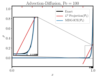
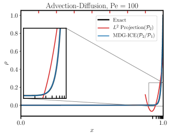
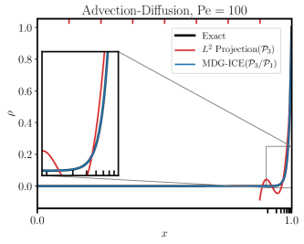
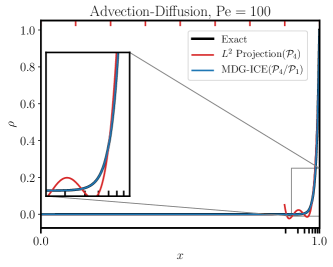
Figure 3.1: Steady, linear advection-diffusion, $\mathrm{Pe}=100$. The $L^{2}$ projection of the exact solution onto a uniform grid consisting of 8 linear line cells is compared for various polynomial degrees to MDG-ICE, which automatically moved the initially uniform grid, indicated by red tick marks, in order to resolve the boundary layer profile, resulting in the adapted grid indicated with black tick marks.

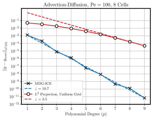
Figure 3.2: Steady, linear advection-diffusion, $\mathrm{Pe}=100$. The rate of convergence with respect to polynomial degree on a log-linear plot is shown, comparing the $L^{2}$ projection onto a uniform grid to MDG-ICE, which automatically moved the initially uniform grid to resolve the boundary layer profile. Reference slopes of $10.7$ and $3.5$ are shown, illustrating the increased rate of convergence achieved using MDG-ICE.

Figure 3.1 shows the MDG-ICE solution to the linear advection-diffusion problem with exact solution (3.2) for $\mathrm{Pe}=100$ as well as the corresponding $L^{2}$ projection of the exact solution onto a uniform grid of 8 linear line cells. The $L^{2}$ projection minimizes the error in the $L^{2}$ norm and therefore provides an upper bound on the accuracy attainable by methods based on a static grid, e.g., DG. By moving the grid to resolve the boundary layer profile, MDG-ICE is able to achieve accurate, oscillation-free, solutions for a range of polynomial degrees.

Figure 3.2 presents the corresponding convergence results with respect to polynomial degree, i.e., $p$-refinement. The rate of convergence of MDG-ICE with respect to polynomial degree is compared to the $L^{2}$ projection of the exact solution onto a uniform grid. These results confirm that MDG-ICE resolves sharp boundary layers with enhanced accuracy compared to static grid methods. Even for a $\mathcal{P}_{1}$ approximation, MDG-ICE provides nearly two orders of magnitude improved accuracy compared to the best approximation available on a uniform grid, a gap that only widens at higher polynomial degrees. The MDG-ICE error is plotted on a log-linear plot, with a reference slope of $10.7$, indicating spectral convergence. This shows that the $r$-adaptivity provided by MDG-ICE enhances the effectiveness of $p$-refinement, even in the presence of initially under-resolved flow features. This results demonstrates the enhanced accuracy of MDG-ICE for resolving initially under-resolved flow features using high-order finite element approximation in comparison to traditional static grid methods, such as DG.

3.2 Space-time Burgers viscous shock formation

For a space-time Burgers flow, described in Section 2.1.2, a shock will form at time $t=t_{s}=0.5$ for the following initial conditions

$$y\left(x,t=0\right)=\frac{1}{2\pi t_{s}}\sin\left(2\pi x\right)+y_{\infty},$$ (3.3)

where $y_{\infty}=0.2$ is the freestream velocity. The space-time solution was initialized by extruding the temporal inflow condition, given by Equation (3.3), throughout the space-time domain.

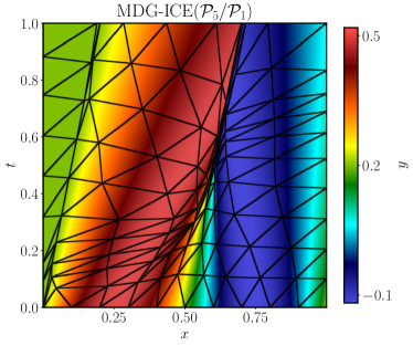
(a) Inviscid MDG-ICE$\left(\mathcal{P}_{5}/\mathcal{P}_{1}\right)$ space-time solution computed using 200 triangle elements.

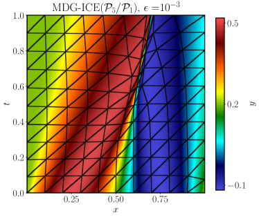
(b) MDG-ICE$\left(\mathcal{P}_{5}/\mathcal{P}_{1}\right)$ space-time solution for $\epsilon=10^{-3}$ computed using 200 triangle elements.

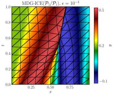
(c) MDG-ICE$\left(\mathcal{P}_{5}/\mathcal{P}_{1}\right)$ space-time solution for $\epsilon=10^{-4}$ computed using 200 triangle elements.

Figure 3.3: Space-time Burgers shock formation: inviscid, viscous $\left(\epsilon=10^{-3}\right)$, and viscous $\left(\epsilon=10^{-4}\right)$ solutions computed using $\mathcal{P}_{5}$ linear triangle elements without shock capturing. Instead, the viscous shock was resolved via anisotropic space-time $r$-adaptivity. The solver was initialized by extruding the initial condition at $t=0$ in time.

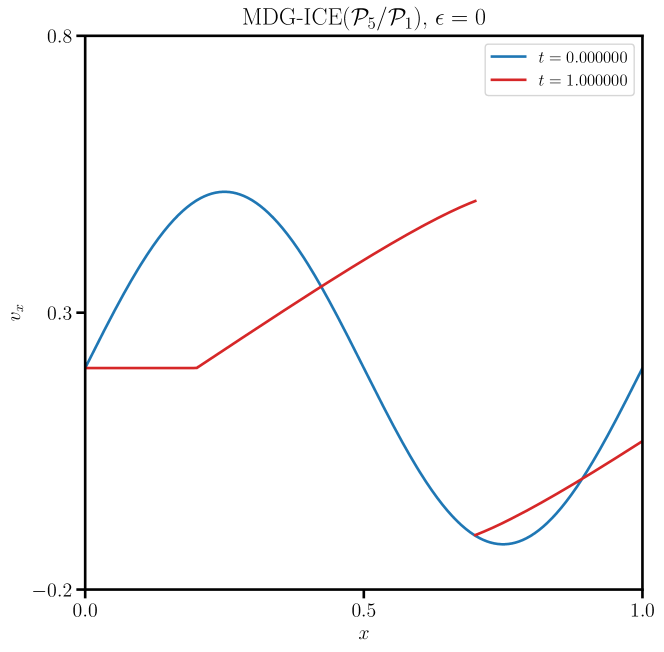
(a) Inviscid MDG-ICE$\left(\mathcal{P}_{5}/\mathcal{P}_{1}\right)$ at $t=0$ and $t=1$. The corresponding space-time solution is shown in Figure 3.3a.

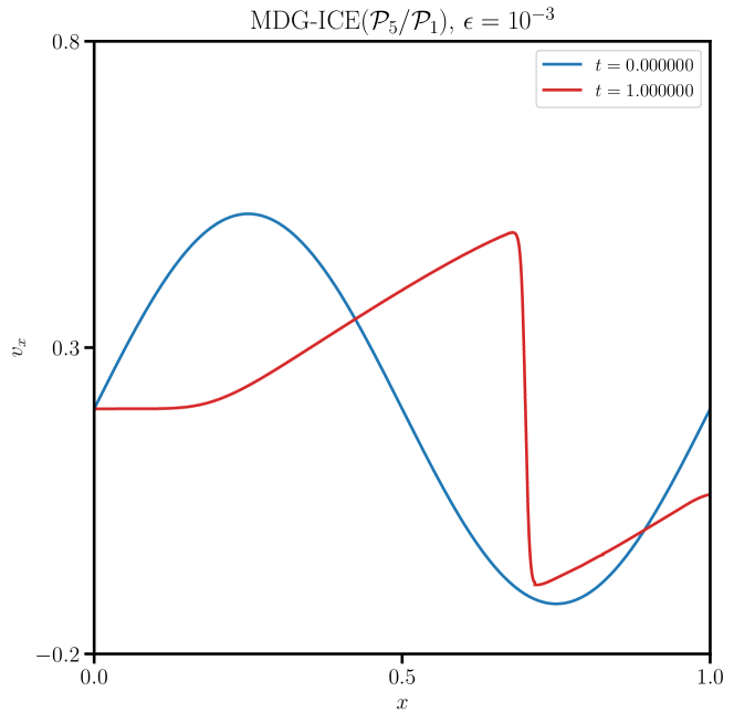
(b) Viscous MDG-ICE$\left(\mathcal{P}_{5}/\mathcal{P}_{1}\right)$ with $\epsilon={1}\mathrm{e}{-3}$ at $t=0$ and $t=1$ . The corresponding space-time solution is shown in Figure 3.3b.

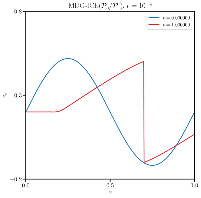
(c) Viscous MDG-ICE$\left(\mathcal{P}_{5}/\mathcal{P}_{1}\right)$ with $\epsilon={1}\mathrm{e}{-4}$ at $t=0$ and $t=1$ . The corresponding space-time solution is shown in Figure 3.3c.

Figure 3.4: Burgers shock formation one-dimensional profiles at $t=0$ and $t=1$: inviscid, viscous $\left(\epsilon=10^{-3}\right)$, and viscous $\left(\epsilon=10^{-4}\right)$ solutions computed using $\mathcal{P}_{5}$ linear triangle elements without shock capturing. The corresponding space-time solutions are shown in Figure 3.3.

Figure 3.3 presents the space-time Burgers shock formation solutions for an inviscid flow, a viscous flow with $\epsilon=10^{-3}$, and a viscous flow with $\epsilon=10^{-4}$. Figure 3.4 presents the corresponding one-dimensional profiles at $t=0$ and $t=1$. The space-time solutions were initialized by extruding the inflow condition, given by Equation (3.3), at $t=0$ in time. The initial simplicial grid was generated by converting a uniform $10\times 10$ quadrilateral grid into triangles.

In the inviscid case, MDG-ICE fits the point of shock formation and tracks the shock at the correct speed. In addition to the shock, the inviscid flow solution has a derivative discontinuity that MDG-ICE also detects and tracks at the correct speed of $0.2$. For the two viscous flow cases, $\epsilon=10^{-3}$ and $\epsilon=10^{-4}$, MDG-ICE accurately resolves each viscous shock as a sharp, yet smooth, profile by adjusting the grid geometry, without modifying the grid topology. This case demonstrates the inherent ability of MDG-ICE to achieve anisotropic space-time $r$-adaptivity for unsteady flow problems.

3.3 Mach 5 viscous bow shock

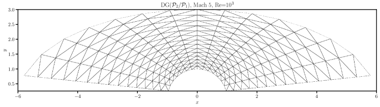
(a) 392 linear triangle cells

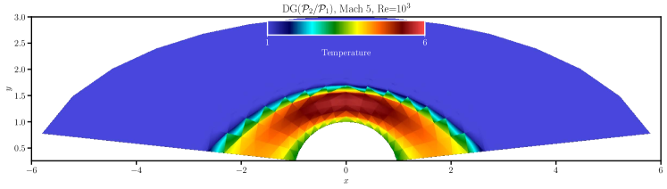
(b) 392 linear $\mathcal{P}_{2}$ triangle cells

Figure 3.5: The initial linear grid and temperature field corresponding to a shock captured DG($\mathcal{P}_{2}/\mathcal{P}_{1}$) solution for the viscous Mach 5 bow shock at $\mathrm{Re}=10^{3}$.

(a) 400 isoparametric $\mathcal{P}_{4}$ triangle cells

(b) 400 isoparametric $\mathcal{P}_{4}$ triangle cells

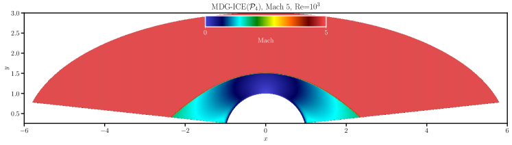
(c) 400 isoparametric $\mathcal{P}_{4}$ triangle cells

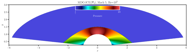
(d) 400 isoparametric $\mathcal{P}_{4}$ triangle cells

Figure 3.6: The MDG-ICE solution computed using $\mathcal{P}_{4}$ isoparametric triangle elements for the viscous Mach 5 bow shock at $\mathrm{Re}=10^{3}$. The MDG-ICE grid was initialized by projecting the linear triangle grid shown in Figure 3.5a to the closest point on the boundary of the domain. The MDG-ICE field variables were initialized by cell averaging the interpolated the DG($\mathcal{P}_{2}/\mathcal{P}_{1}$) solution shown in Figure 3.5b. The MDG-ICE flux variables were initialized to zero for consistency with the initial piecewise constant field variables. The location of the shock along the line $x=0$ was computed as $y=1.49995$ for a stand-off distance of $0.49995$.

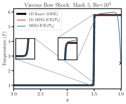
(a) The temperature sampled along $x=0$. The exact temperature at the stagnation point, $T=2.5$, is marked with the symbol $\times$.

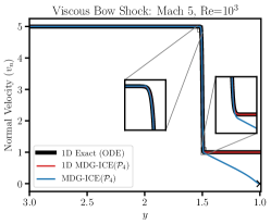
(b) The normal velocity, $v_{n}=0$, sampled along $x=0$. The exact normal velocity at the stagnation point, $v_{n}=0$, is marked with the symbol $\times$.

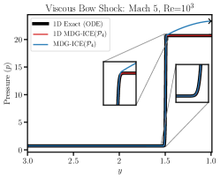
(c) The pressure, $p$, sampled along $x=0$. The exact pressure at the stagnation point for an inviscid flow, $p\approx 23.324$, is marked with the symbol $\times$.

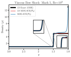
(d) The density, $\rho$, sampled along $x=0$. The density at the stagnation point, computed using the stagnation pressure corresponding to an inviscid flow, $\rho\approx 13.061389724919298$, is marked with the symbol $\times$.

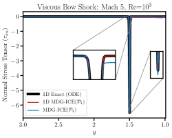
(e) The normal component of the normal viscous stress tensor, $\tau_{nn}$, sampled along $x=0$.

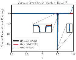
(f) The normal thermal heat flux, $q_{n}$, sampled along $x=0$.

Figure 3.7: Centerline profiles of temperature and normal velocity for the viscous Mach 5 bow shock at $\mathrm{Re}=10^{3}$ computed with MDG-ICE($\mathcal{P}_{4}$) compared to ODE and MDG-ICE($\mathcal{P}_{4}$) approximations of the exact solution for the corresponding one-dimensional viscous shock. The one-dimensional MDG-ICE($\mathcal{P}_{4}$) approximation was computed using 16 isoparametric line cells. The location of the shock was computed as $y=1.49995$ for a stand-off distance of $0.49995$.

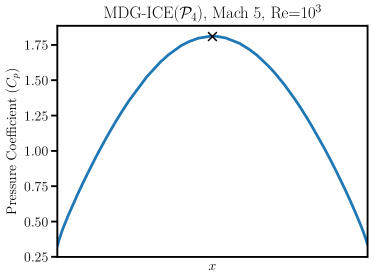
(a) The pressure coefficient, $C_{p}$, sampled at each degree of freedom on the surface of the cylinder. The exact pressure coefficient at the stagnation point for an inviscid flow, $C_{p}\approx 1.8087699607027568$, is marked with the symbol $\times$.

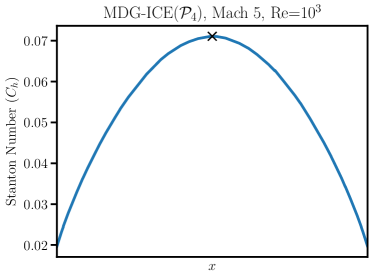
(b) The Stanton number sampled at each degree of freedom on the surface of the cylinder. The computed Stanton number at the stagnation point is marked with the symbol $\times$.

Figure 3.8: Pressure coefficient and Stanton number for the viscous Mach 5 bow shock at $\mathrm{Re}=10^{3}$ computed with MDG-ICE($\mathcal{P}_{4}$) .

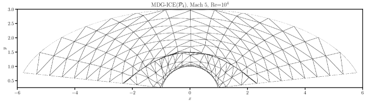
(a) 527 isoparametric $\mathcal{P}_{4}$ triangle cells

(b) 527 isoparametric $\mathcal{P}_{4}$ triangle cells

(c) 527 isoparametric $\mathcal{P}_{4}$ triangle cells

(d) 527 isoparametric $\mathcal{P}_{4}$ triangle cells

Figure 3.9: The MDG-ICE solution computed using $\mathcal{P}_{4}$ isoparametric triangle elements for the viscous Mach 5 bow shock at $\mathrm{Re}=10^{4}$. The MDG-ICE solution was initialized from the MDG-ICE solution at $\mathrm{Re}=10^{3}$ shown in Figure 3.5a. The location of the shock along the line $x=0$ was computed as $y=1.48437$ for a stand-off distance of $0.48437$.

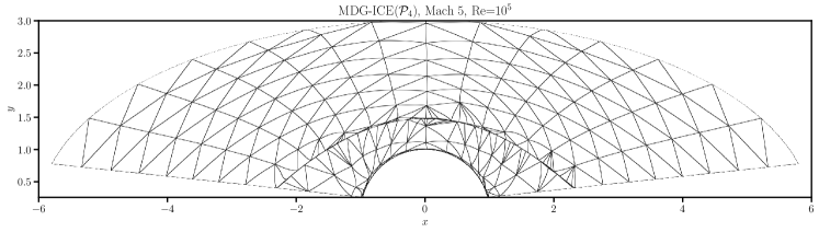
(a) 768 isoparametric $\mathcal{P}_{4}$ triangle cells

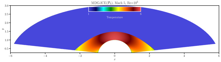
(b) 768 isoparametric $\mathcal{P}_{4}$ triangle cells

(c) 768 isoparametric $\mathcal{P}_{4}$ triangle cells

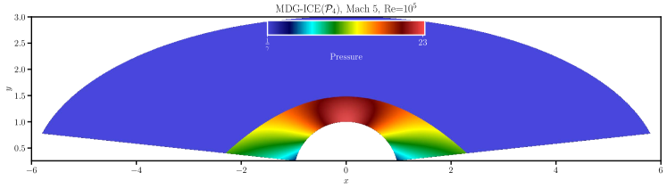
(d) 768 isoparametric $\mathcal{P}_{4}$ triangle cells

Figure 3.10: The MDG-ICE solution computed using $\mathcal{P}_{4}$ isoparametric triangle elements for the viscous Mach 5 bow shock at $\mathrm{Re}=10^{5}$. The MDG-ICE solution was initialized from the MDG-ICE solution at $\mathrm{Re}=10^{4}$ shown in Figure 3.5a. The location of the shock along the line $x=0$ was computed as $y=1.4809125$ for a stand-off distance of $0.4809125$.

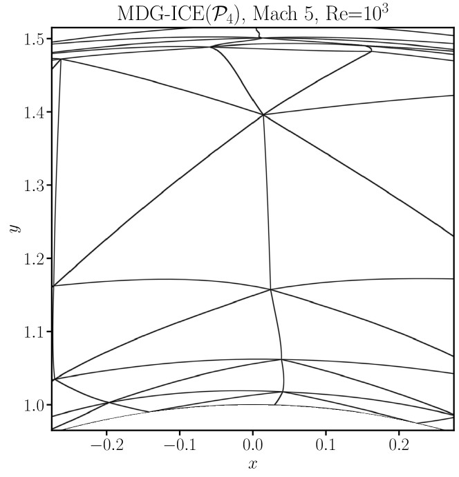
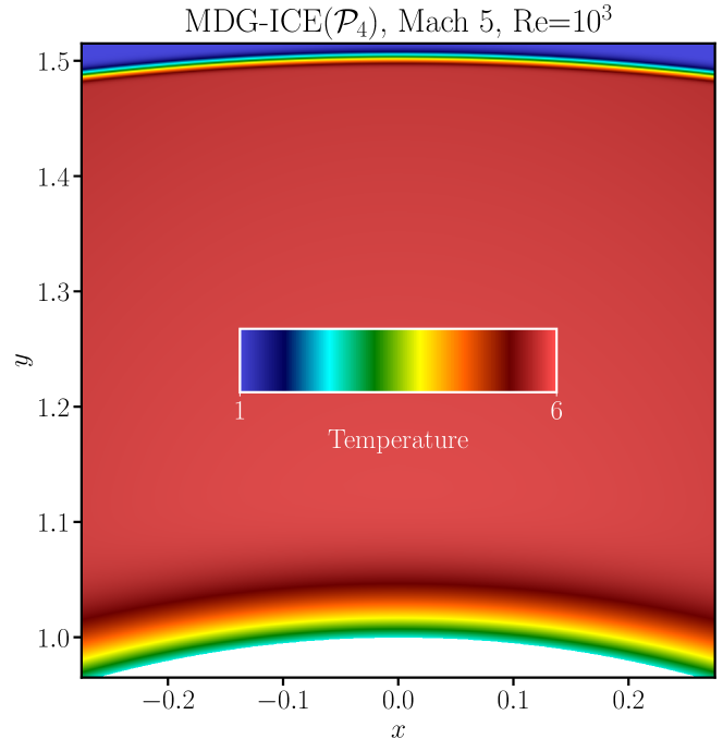
(a) The final grid and temperature fields of the MDG-ICE$\left(\mathcal{P}_{4}\right)$ solution computed using 400 $\mathcal{P}_{4}$ isoparametric triangle elements for the viscous Mach 5 bow shock at $10^{3}$ $\mathrm{Re}$ shown in Figure 3.6a and Figure 3.6b respectively.

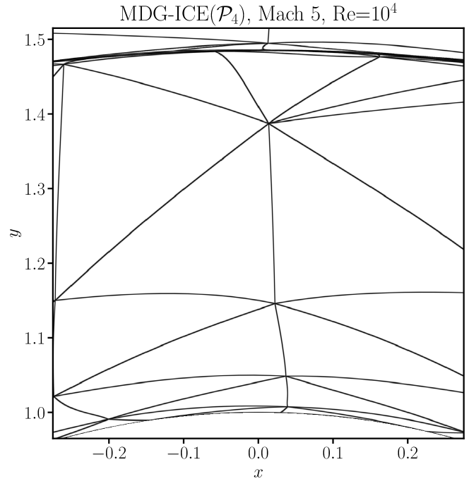
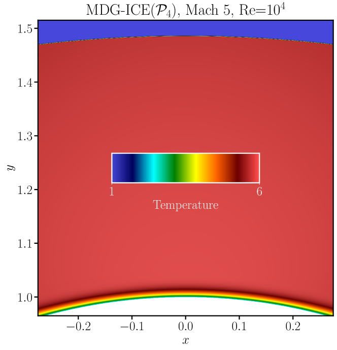
(b) The final grid and temperature fields of the MDG-ICE$\left(\mathcal{P}_{4}\right)$ solution computed using 527 $\mathcal{P}_{4}$ isoparametric triangle elements for the viscous Mach 5 bow shock at $10^{4}$ $\mathrm{Re}$ shown in Figure 3.9a and Figure 3.9b.

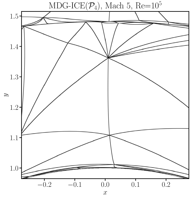
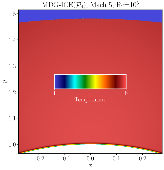
(c) The final grid and temperature fields of the MDG-ICE$\left(\mathcal{P}_{4}\right)$ solution computed using 768 $\mathcal{P}_{4}$ isoparametric triangle elements for the viscous Mach 5 bow shock at $10^{5}$ $\mathrm{Re}$ shown in Figure 3.10a and Figure 3.10b.

Figure 3.11: The final grid and temperature fields corresponding to the MDG-ICE solution computed using $\mathcal{P}_{4}$ isoparametric triangle elements for the viscous Mach 5 bow shock at $\mathrm{Re}=10^{3}$, $\mathrm{Re}=10^{4}$, and $\mathrm{Re}=10^{5}$. Local edge refinement was used to adaptively split highly anisotropic elements within the viscous structures as they were resolved by MDG-ICE.

The viscous MDG-ICE discretization is applied to a compressible Navier-Stokes flow, described in Section (2.1.3), and used to approximate the solution to a supersonic viscous flow over a cylinder in two dimensions. The solution is characterized by the Reynolds number $\mathrm{Re}$, and the freestream Mach number $\mathrm{M}_{\infty}$. The Reynolds number is defined as,

$$\mathrm{Re}=\frac{\rho vL}{\mu},$$ (3.4)

where $L$ is the characteristic length. The freestream Mach number is defined $\mathrm{M}_{\infty}=\frac{v_{\infty}}{c_{\infty}}$

$$\mathrm{M}_{\infty}=\frac{v_{\infty}}{c_{\infty}},$$ (3.5)

where $v_{\infty}$ is the freestream velocity, $c_{\infty}=\sqrt{\nicefrac{{\gamma P_{\infty}}}{{\rho_{\infty}}}}$ is the freestream speed of sound, $P_{\infty}$ is the freestream pressure, and $\rho_{\infty}$ is the freestream density. In this work we consider Mach 5 flows at Reynolds numbers of $10^{3}$, $10^{4}$, and $10^{5}$ traveling in the $\left(0,-1\right)$ direction, i.e., from top to bottom in Figure 3.5 , Figure 3.6, Figure 3.9, and Figure 3.10. Supersonic inflow and outflow boundary conditions are applied at the ellipse and outflow planes respectively. An isothermal no-slip wall is specified at the surface of the cylinder of radius $r=1$ centered at the origin. The temperature at the isothermal wall is given as $T_{\mathrm{wall}}=2.5T_{\infty}$, where $T_{\infty}$ is the freestream temperature.

Figure 3.6 presents the MDG-ICE($\mathcal{P}_{4}$) solution at $\mathrm{Re}=10^{3}$ computed on a grid of $400$ isoparametric triangle elements. The MDG-ICE($\mathcal{P}_{4}$) solution was initialized by interpolating the DG($\mathcal{P}_{2}$) field variables and the corresponding grid. Figure 3.5a shows the grid consisting of 392 linear triangle elements that was used to initialize the MDG-ICE($\mathcal{P}_{4}$) by interpolating the field variables. The high-order isoparametric boundary faces were initialized by projecting to closest point on the boundary of the domain via the boundary operator (2.80). The MDG-ICE($\mathcal{P}_{4}$) field variables were initialized by cell averaging the interpolated DG($\mathcal{P}_{2}$) solution shown in Figure 3.5b. The MDG-ICE auxiliary variable, with spatial components given by (2.47), were initialized to zero for consistency with the initial piecewise constant field variables. As the MDG-ICE solution converged, the previously uniformly distributed points were relocated in order to resolve the viscous shock. This resulted in a loss of resolution downstream, which was conveniently handled via local edge refinement where highly anisotropic elements were adaptively split as the viscous structures were resolved. Although this was unnecessary for maintaining a valid solution, i.e., field variables that are finite and grid composed of only cells with a positive determinant of the Jacobian, we found it sufficient for maintaining a reasonable grid resolution, as compared to the initial grid resolution downstream of the shock. The location of the shock along the line $x=0$, estimated as the location corresponding to the minimum normal heat flux, was computed as $y=1.49995$, giving a stand-off distance of $0.49995$.

In one dimension, the viscous shock is described by a system of ordinary differential equations that can be solved numerically, cf. ^{94, 93} for details. We use this solution to verify that the viscous MDG-ICE formulation predicts the correct viscous shock profile when diffusive effects are prominent, i.e., at low Reynolds number. Figure 3.7 presents a comparison of an approximation of the exact solution for a one-dimensional viscous shock to the centerline profiles of the Mach 5 bow shock at $\mathrm{Re}=10^{3}$ for the following variables: temperature, $T$, normal velocity, $v_{n}$, pressure, $p$, density, $\rho$, normal component of the normal viscous stress tensor, $\tau_{nn}$, and normal heat flux, $q_{n}$, where the normal is taken to be in the streamwise direction.

As expected, the one-dimensional profiles deviate from the two-dimensional bow shock centerline profiles downstream of the viscous shock. The one-dimensional solution assumes the viscous and diffusive fluxes are zero outside of the shock. This is not the case for the two-dimensional bow shock geometry where the blunt body and corresponding boundary layer produce gradients in the solution downstream of the shock. For density, in which case the diffusive flux is zero, the jump across the viscous shock is directly comparable to the one-dimensional solution. We also directly compare the exact solution to a one-dimensional viscous shock profile computed by MDG-ICE($\mathcal{P}_{4}$) using 16 isoparametric line cells. Figure 3.7d shows that MDG-ICE accurately reproduces the exact shock structure of density profile with only a few high-order anisotropic curvilinear cells.

For reference, the exact and approximate values at the stagnation point are marked on the centerline plots with the symbol $\times$. An approximate value corresponding to the inviscid solution was used when the exact value for the viscous flow was unavailable, e.g., the stagnation pressure marked in Figure 3.7c. Although the analytic stagnation pressure for a inviscid flow neglects viscous effects, it is not expected to differ significantly from the value corresponding to the viscous solution for the problem considered here, as shown in Table 1 in the work of Williams et al. ⁹⁵.

We also report the pressure coefficient and the Stanton number, sampled at the degrees of freedom, on the cylindrical, no-slip, isothermal surface. The pressure coefficient at the surface is defined as

$$C_{p}=\frac{p-p_{\infty}}{\frac{1}{2}\rho_{\infty}v_{\infty}^{2}},$$ (3.6)

where $p_{\infty}$, $\rho_{\infty}$, and $v_{\infty}$ are the freestream pressure, density, and velocity respectively. The Stanton number at the surface is defined as

$$C_{h}=\frac{q_{\mathrm{n}}}{c_{p}\rho_{\infty}v_{\infty}\left(T_{t,\infty}-T_{\mathrm{wall}}\right)},$$ (3.7)

where $q_{n}$ is the normal heat flux, $T_{\mathrm{wall}}$ is the wall temperature, and $T_{t,\infty}$ is the freestream stagnation temperature. In Figure 3.8a the pressure coefficient on the cylindrical surface is plotted and the exact pressure coefficient at the stagnation point for an inviscid flow, $C_{p}\approx 1.8087699607027568$, is marked with the symbol $\times$.

In order to compute solutions at higher Reynolds numbers, continuation of the freestream viscosity, $\mu_{\infty}$ was employed. Figure 3.9 presents the MDG-ICE($\mathcal{P}_{4}$) solution at $\mathrm{Re}=10^{4}$ computed on a grid of $527$ isoparametric triangle elements, which was initialized from the $\mathrm{Re}=10^{3}$ MDG-ICE($\mathcal{P}_{4}$) solution. Figure 3.9 presents the MDG-ICE($\mathcal{P}_{4}$) solution at $\mathrm{Re}=10^{5}$ computed on a grid of $768$ isoparametric triangle elements, which was initialized from the $\mathrm{Re}=10^{4}$ MDG-ICE($\mathcal{P}_{4}$) solution. As in the $\mathrm{Re}=10^{3}$ case, local edge refinement was used to adaptively split highly anisotropic elements within the viscous structures as they were resolved by MDG-ICE. At these higher Reynolds numbers, local refinement was necessary to maintain a valid grid. In addition to the splitting of highly anisotropic cells, local edge refinement was also applied to cells in which the determinant of the Jacobian became non-positive.

Figure 3.11 compares the MDG-ICE($\mathcal{P}_{4}$) solutions directly downstream of the viscous shock at $\mathrm{Re}=10^{3}$, $\mathrm{Re}=10^{4}$, and $\mathrm{Re}=10^{5}$. By adapting the grid to the flow field, MDG-ICE is able to simultaneously resolve the thin viscous structure over a range of Reynolds numbers. As the MDG-ICE solution converges, elements within regions that contain strong gradients become highly anisotropic and warp nonlinearly to conform to both the curved shock geometry and efficiently resolve the flow around the curved blunt body. Thus, unlike a posteriori anisotropic mesh adaptation, MDG-ICE achieves high-order anisotropic curvilinear $r$-adaptivity as an intrinsic part of the solver. Furthermore, MDG-ICE automatically repositions the nodes in order to resolve the flow field over different length scales as the Reynolds number is increased from $10^{3}$ to $10^{5}$. As such, MDG-ICE overcomes another challenge associated with a posteriori anisotropic mesh adaptation which produces regions of excessive refinement on the scale of the coarse mesh cell size and therefore must rely on grid coarsening to limit the region of refinement to the more appropriate length scale corresponding to the feature under consideration.

4 Conclusions and future work

The Moving Discontinuous Galerkin Method with Interface Condition Enforcement (MDG-ICE) has been applied to viscous flow problems, involving both linear and nonlinear viscous fluxes, where it was shown to detect and resolve previously under-resolved flow features. In the case of linear advection-diffusion, MDG-ICE adapted the grid to resolve the initially under-resolved boundary layer, thereby achieving spectral convergence and a more accurate solution than the best possible approximation on a uniform static grid, which is given by the $L^{2}$ projection of the exact solution. Unsteady flows were computed using a space-time formulation where viscous structures were automatically resolved via anisotropic space-time $r$-adaptivity. High speed compressible Navier-Stokes solutions for a viscous Mach 5 bow shock at a Reynolds numbers of $10^{3}$, $10^{4}$, and $10^{5}$ were presented. The viscous MDG-ICE formulation was shown to produce the correct viscous shock profile in one dimension for a Mach 5 flow at $\mathrm{Re}=10^{3}$. The one-dimensional viscous shock profile was compared to the centerline profile of the two-dimensional MDG-ICE solution where it was shown to accurately compute both the shock profile and boundary layer profile simultaneously using only a few high-order anisotropic curved cells within each region and thus overcoming an ongoing limitation of anisotropic mesh adaptation. Local edge refinement was used to adaptively split highly anisotropic elements within the viscous structures as they were resolved by MDG-ICE. Finally, MDG-ICE is a consistent discretization of the governing equations that does not introduce low-order errors via artificial stabilization or limiting and treats the discrete grid as a variable.

It should be noted that the internal structure of a viscous shock may not be adequately described by the compressible Navier-Stokes equations due to non-equilibrium effects ⁹⁶, an issue surveyed by Powers et al. ⁹⁷. While in the present work MDG-ICE was shown to provide highly accurate solutions to the compressible Navier-Stokes equations, future work will apply MDG-ICE to an improved multi-scale model that incorporates physical effects more adequately described by the kinetic theory of gases ⁹⁸. MDG-ICE is a promising method to apply within such a framework due to its ability to isolate regions in which enhanced physical modeling is required.

In future work, we will also develop a least-squares MDG-ICE formulation with optimal test functions by applying the DPG methodology of Demkowicz and Gopalakrishnan ^{58, 59, 65}. Using this approach we will demonstrate high-order convergence for both linear and nonlinear problems. We also plan to mitigate the need for local $h$-refinement by considering alternative methods for maintaining grid validity. We will explore adaptively increasing the order of the local polynomial approximation for cells within thin internal and boundary layers. For instance, Chan et al. ^{94, 85} used a combination of $h$ and $p$ refinement to resolve viscous shocks. In their adaptive strategy, $h-$refinement is used until the local grid resolution is on the order of the viscous scale, at which point $p$-refinement is used to further enhance accuracy. Additionally, scaling the regularization by the inverse of volume of the cell, an approach used by Zahr et al. ^{31, 32} may also be effective for maintaining grid validity at higher Reynolds numbers. Ultimately, we plan on maintaining grid validity by incorporating smoothing, or untangling, into the projection operator, Equation (2.80), which enforces the geometric boundary conditions.

References

- 1 Bassi F., Rebay S.. A high-order accurate discontinuous finite element method for the numerical solution of the compressible Navier–Stokes equations. Journal of Computational Physics. 1997;131(2):267–279.
- 2 Bassi F., Rebay S.. High-order accurate discontinuous finite element solution of the 2D Euler equations. Journal of Computational Physics. 1997;138(2):251–285.
- 3 Cockburn B., Shu C.-W.. The Runge–Kutta discontinuous Galerkin method for conservation laws V: multidimensional systems. Journal of Computational Physics. 1998;141(2):199–224.
- 4 Cockburn B., Karniadakis G.E., Shu C.-W.. The development of discontinuous Galerkin methods. In: Springer 2000 (pp. 3–50).
- 5 Arnold D.N., Brezzi F., Cockburn B., Marini L.D.. Unified analysis of discontinuous Galerkin methods for elliptic problems. SIAM Journal on Numerical Analysis. 2002;39(5):1749–1779.
- 6 Hartmann R., Houston P.. Adaptive discontinuous Galerkin finite element methods for the compressible Euler equations. Journal of Computational Physics. 2002;183(2):508–532.
- 7 Fidkowski K.J., Oliver T.A, Lu J., Darmofal D.L.. p-Multigrid solution of high-order discontinuous Galerkin discretizations of the compressible Navier–Stokes equations. Journal of Computational Physics. 2005;207(1):92–113.
- 8 Hesthaven J. S., Warburton T.. Nodal discontinuous Galerkin methods: algorithms, analysis, and applications. Springer Science & Business Media; 2007.
- 9 Persson P-O, Peraire J.. Newton-GMRES preconditioning for discontinuous Galerkin discretizations of the Navier–Stokes equations. SIAM Journal on Scientific Computing. 2008;30(6):2709–2733.
- 10 Hartmann R., Leicht T.. Higher order and adaptive DG methods for compressible flows. In: Deconinck H., ed. VKI LS 2014-03: 37th Advanced VKI CFD Lecture Series: Recent developments in higher order methods and industrial application in aeronautics, Dec. 9-12, 2013, Von Karman Institute for Fluid Dynamics, Rhode Saint Genèse, Belgium 2014. Retrieved from https://ganymed.math.uni-heidelberg.de/~hartmann/publications/2014/HL14a.pdf.
- 11 Liu J.-G., Shu C.-W.. A high-order discontinuous Galerkin method for 2D incompressible flows. Journal of Computational Physics. 2000;160(2):577–596.
- 12 Bassi F., Crivellini A., Di Pietro D. A., Rebay S.. An implicit high-order discontinuous Galerkin method for steady and unsteady incompressible flows. Computers & Fluids. 2007;36(10):1529–1546.
- 13 Rhebergen S., Cockburn B.. A space–time hybridizable discontinuous Galerkin method for incompressible flows on deforming domains. Journal of Computational Physics. 2012;231(11):4185–4204.
- 14 Lv Y., Ihme M.. Discontinuous Galerkin method for multicomponent chemically reacting flows and combustion. Journal of Computational Physics. 2014;270:105–137.
- 15 Johnson R. F., Goodwin G. B., Corrigan A. T., Kercher A., Chelliah H. K.. Discontinuous-Galerkin Simulations of Premixed Ethylene-Air Combustion in a Cavity Combustor. In: AIAA , ed. 2019 AIAA SciTech Forum, ; 2019. AIAA-2019-1444.
- 16 Johnson R.F., Kercher A.D.. A Conservative Discontinuous Galerkin Discretization for the Total Energy Formulation of the Reacting Navier Stokes Equations. arXiv preprint arXiv:1910.10544. 2019;.
- 17 Wang Z.J., Fidkowski K., Abgrall R., et al. High-Order CFD Methods: Current Status and Perspective. International Journal for Numerical Methods in Fluids. 2013;.
- 18 Corrigan A., Kercher A.D., Kessler D.A.. A Moving Discontinuous Galerkin Finite Element Method for Flows with Interfaces. NRL/MR/6040–17-9765: U.S. Naval Research Laboratory; 2017. https://apps.dtic.mil/dtic/tr/fulltext/u2/1042881.pdf.
- 19 Corrigan A., Kercher A.D., Kessler D.A.. A Moving Discontinuous Galerkin Finite Element Method for Flows with Interfaces. International Journal for Numerical Methods in Fluids. 2019;89(9):362-406.
- 20 Lowrie R., Roe P., Leer B.. A space-time discontinuous Galerkin method for the time-accurate numerical solution of hyperbolic conservation laws. In: AIAA , ed. 12th Computational Fluid Dynamics Conference, ; 1995. AIAA-995-1658.
- 21 Lowrie R.B., Roe P.L., Van Leer B.. Space-time methods for hyperbolic conservation laws. In: Springer 1998 (pp. 79–98).
- 22 Corrigan A., Kercher A., Kessler D.. The Moving Discontinuous Galerkin Method with Interface Condition Enforcement for Unsteady Three-Dimensional Flows. In: AIAA , ed. 2019 AIAA SciTech Forum, ; 2019. AIAA-2019-0642.
- 23 Corrigan A., Kercher A., Kessler D., Wood-Thomas D.. Application of the Moving Discontinuous Galerkin Method with Interface Condition Enforcement to Shocked Compressible Flows. In: AIAA , ed. 2018 AIAA AVIATION Forum, ; 2018. AIAA-2018-4272.
- 24 Corrigan A., Kercher A., Kessler D., Wood-Thomas D.. Convergence of the Moving Discontinuous Galerkin Method with Interface Condition Enforcement in the Presence of an Attached Curved Shock. In: AIAA , ed. 2019 AIAA AVIATION Forum, ; 2019. AIAA-2019-3207.
- 25 Moretti G.. Thirty-six years of shock fitting. Computers & Fluids. 2002;31(4):719–723.
- 26 Salas M.D.. A shock-fitting primer. CRC Press; 2009.
- 27 Salas M.D.. A brief history of shock-fitting. In: Springer 2011 (pp. 37–53).
- 28 Zahr M. J., Persson P.-O.. An optimization-based approach for high-order accurate discretization of conservation laws with discontinuous solutions. ArXiv e-prints. 2017;.
- 29 Zahr M.J., Persson P.-O.. An Optimization Based Discontinuous Galerkin Approach for High-Order Accurate Shock Tracking. In: AIAA , ed. 2018 AIAA Aerospace Sciences Meeting, ; 2018. AIAA-2018-0063.
- 30 Zahr M.J., Persson P-O. An optimization-based approach for high-order accurate discretization of conservation laws with discontinuous solutions. Journal of Computational Physics. 2018;.
- 31 Zahr M. J., Shi A., Persson P.-O.. Implicit shock tracking using an optimization-based, -adaptive, high-order discontinuous Galerkin method. ArXiv e-prints. 2019;.
- 32 Zahr M. J., Shi A., Persson P.-O.. An -adaptive, high-order discontinuous Galerkin method for flows with attached shocks. In: AIAA , ed. 2020 AIAA SciTech Forum, ; 2020. AIAA-2020-0537.
- 33 Tam A., Ait-Ali-Yahia D., Robichaud M.P., Moore M., Kozel V., Habashi W.G.. Anisotropic mesh adaptation for 3D flows on structured and unstructured grids. Computer Methods in Applied Mechanics and Engineering. 2000;189(4):1205–1230.
- 34 Pain C.C., Umpleby A.P., De Oliveira C.R.E., Goddard A.J.H.. Tetrahedral mesh optimisation and adaptivity for steady-state and transient finite element calculations. Computer Methods in Applied Mechanics and Engineering. 2001;190(29-30):3771–3796.
- 35 George P.-L.. Gamanic3d, adaptive anisotropic tetrahedral mesh generator. : Technical Report, INRIA; 2002.
- 36 Bottasso C. L.. Anisotropic mesh adaption by metric-driven optimization. International Journal for Numerical Methods in Engineering. 2004;60(3):597–639.
- 37 Li X., Shephard M. S., Beall M. W.. 3D anisotropic mesh adaptation by mesh modification. Computer methods in applied mechanics and engineering. 2005;194(48-49):4915–4950.
- 38 Jones W., Nielsen E., Park M.. Validation of 3D adjoint based error estimation and mesh adaptation for sonic boom prediction. In: AIAA , ed. 44th AIAA Aerospace Sciences Meeting and Exhibit, :1150; 2006. AIAA-2006-1150.
- 39 Dobrzynski C., Frey P.. Anisotropic Delaunay mesh adaptation for unsteady simulations. In: Springer 2008 (pp. 177–194).
- 40 Compere G., Remacle J.-F., Jansson J., Hoffman J.. A mesh adaptation framework for dealing with large deforming meshes. International journal for numerical methods in engineering. 2010;82(7):843–867.
- 41 Loseille A., Löhner R.. Anisotropic adaptive simulations in aerodynamics. In: AIAA , ed. 48th AIAA Aerospace Sciences Meeting Including the New Horizons Forum and Aerospace Exposition, :169; 2010. AIAA-2010-0169.
- 42 Loseille A., Löhner R.. Boundary layer mesh generation and adaptivity. In: AIAA , ed. 49th AIAA Aerospace Sciences Meeting including the New Horizons Forum and Aerospace Exposition, :894; 2011. AIAA-2011-0894.
- 43 Löhner R.. Matching semi-structured and unstructured grids for Navier-Stokes calculations. In: AIAA , ed. 11th Computational Fluid Dynamics Conference, :3348; 1993. AIAA-1993-3348.
- 44 Löhner R.. Generation of unstructured grids suitable for RANS calculations. In: Springer 2000 (pp. 153–163).
- 45 Pirzadeh S.. Viscous unstructured three-dimensional grids by the advancing-layers method. In: AIAA , ed. 32nd Aerospace Sciences Meeting and Exhibit, :417; 1994. AIAA-1994-0417.
- 46 Marcum D. L.. Adaptive unstructured grid generation for viscous flow applications. AIAA journal. 1996;34(11):2440–2443.
- 47 Garimella R. V., Shephard M. S.. Boundary layer mesh generation for viscous flow simulations. International Journal for Numerical Methods in Engineering. 2000;49(1-2):193–218.
- 48 Bottasso C. L., Detomi D.. A procedure for tetrahedral boundary layer mesh generation. Engineering with Computers. 2002;18(1):66–79.
- 49 Ito Y., Nakahashi K.. Unstructured Mesh Generation for Viscous Flow Computations.. In: :367–377; 2002.
- 50 Ito Y., Shih A., Soni B., Nakahashi K.. An approach to generate high quality unstructured hybrid meshes. In: AIAA , ed. 44th AIAA Aerospace Sciences Meeting and Exhibit, :530; 2006. AIAA-2006-0530.
- 51 Aubry R., Löhner R.. Generation of viscous grids at ridges and corners. International journal for numerical methods in engineering. 2009;77(9):1247–1289.
- 52 Fidkowski K. .J, Darmofal D. .L. Review of output-based error estimation and mesh adaptation in computational fluid dynamics. AIAA journal. 2011;49(4):673–694.
- 53 Yano M., Darmofal D. L.. An optimization-based framework for anisotropic simplex mesh adaptation. Journal of Computational Physics. 2012;231(22):7626–7649.
- 54 Carson H. A., Allmaras S. R., Galbraith M. C., Darmofal D.L.. Mesh optimization via error sampling and synthesis: An update. In: AIAA , ed. 2020 AIAA SciTech Forum, :87; 2020. AIAA-2020-0087.
- 55 Alauzet F., Loseille A.. A decade of progress on anisotropic mesh adaptation for computational fluid dynamics. Computer-Aided Design. 2016;72:13–39.
- 56 Jiang B.-N., Carey G.F.. Adaptive refinement for least-squares finite elements with element-by-element conjugate gradient solution. International journal for numerical methods in engineering. 1987;24(3):569–580.
- 57 Carey G.F., Pehlivanov A.I.. Local error estimation and adaptive remeshing scheme for least-squares mixed finite elements. Computer methods in applied mechanics and engineering. 1997;150(1-4):125–131.
- 58 Demkowicz L., Gopalakrishnan J.. A class of discontinuous Petrov–Galerkin methods. Part I: The transport equation. Computer Methods in Applied Mechanics and Engineering. 2010;199(23-24):1558–1572.
- 59 Demkowicz L., Gopalakrishnan J.. A class of discontinuous Petrov–Galerkin methods. II. Optimal test functions. Numerical Methods for Partial Differential Equations. 2011;27(1):70–105.
- 60 Demkowicz L., Gopalakrishnan J., Niemi Antti H. A class of discontinuous Petrov–Galerkin methods. Part III: Adaptivity. Applied numerical mathematics. 2012;62(4):396–427.
- 61 Gopalakrishnan J.. Five lectures on DPG methods. arXiv preprint arXiv:1306.0557. 2013;.
- 62 Gopalakrishnan J., Qiu W.. An analysis of the practical DPG method. Mathematics of Computation. 2014;83(286):537–552.
- 63 Carstensen C., Demkowicz L., Gopalakrishnan J.. Breaking spaces and forms for the DPG method and applications including Maxwell equations. Computers & Mathematics with Applications. 2016;72(3):494–522.
- 64 Demkowicz L., Gopalakrishnan J., Keith B.. The DPG-star method. Computers & Mathematics with Applications. 2020;.
- 65 Demkowicz L., Gopalakrishnan J.. Discontinuous Petrov-Galerkin (DPG) method. 15-20: ICES; 2015. Retrieved from https://www.oden.utexas.edu/media/reports/2015/1520.pdf.
- 66 Miller K., Miller R.N.. Moving finite elements. I. SIAM Journal on Numerical Analysis. 1981;18(6):1019–1032.
- 67 Miller K.. Moving finite elements. II. SIAM Journal on Numerical Analysis. 1981;18(6):1033–1057.
- 68 Gelinas R.J., Doss S.K., Miller K.. The moving finite element method: applications to general partial differential equations with multiple large gradients. Journal of Computational Physics. 1981;40(1):202–249.
- 69 Bank R.E., Santos R.F.. Analysis of some moving space-time finite element methods. SIAM journal on numerical analysis. 1993;30(1):1–18.
- 70 Bochev P., Liao G., Pena G.. Analysis and computation of adaptive moving grids by deformation. Numerical Methods for Partial Differential Equations: An International Journal. 1996;12(4):489–506.
- 71 Roe P., Nishikawa H.. Adaptive grid generation by minimizing residuals. International Journal for Numerical Methods in Fluids. 2002;40(1-2):121–136.
- 72 Sanjaya D.P., Fidkowski K.J.. Improving High-Order Finite Element Approximation Through Geometrical Warping. AIAA Journal. 2016;54(12):3994–4010.
- 73 Budd C.J., Huang W., Russell R.D.. Adaptivity with moving grids. Acta Numerica. 2009;18:111–241.
- 74 Huang W., Russell R.D.. Adaptive moving mesh methods. Springer Science & Business Media; 2010.
- 75 Majda A.. Compressible fluid flow and systems of conservation laws in several space variables. Springer Science & Business Media; 2012.
- 76 Persson P-O., Peraire J.. Sub-cell shock capturing for discontinuous Galerkin methods. In: AIAA , ed. 44th AIAA Aerospace Sciences Meeting and Exhibit, ; 2006. AIAA-2006-112.
- 77 Peraire J., Nguyen NC, Cockburn B.. A hybridizable discontinuous Galerkin method for the compressible Euler and Navier-Stokes equations. In: AIAA , ed. 48th AIAA Aerospace Sciences Meeting Including the New Horizons Forum and Aerospace Exposition, ; 2010. AIAA-2010-0363.
- 78 Hansbo A., Hansbo P.. An unfitted finite element method, based on Nitsche’s method, for elliptic interface problems. Computer Methods in Applied Mechanics and Engineering. 2002;191(47):5537–5552.
- 79 Massjung R.. An unfitted discontinuous Galerkin method applied to elliptic interface problems. SIAM Journal on Numerical Analysis. 2012;50(6):3134–3162.
- 80 Mott D. R., Kercher A.D., Adams A., et al. Interface-fitted Simulation of Multi-Material Sheath Flow using MDG-ICE. In: AIAA , ed. 2020 AIAA SciTech Forum, ; 2020. AIAA-2020-0562.
- 81 Cockburn B., Shu C.-W.. The local discontinuous Galerkin method for time-dependent convection-diffusion systems. SIAM Journal on Numerical Analysis. 1998;35(6):2440–2463.
- 82 Broersen D., Stevenson R.. A robust Petrov–Galerkin discretisation of convection–diffusion equations. Computers & Mathematics with Applications. 2014;68(11):1605–1618.
- 83 Broersen D., Stevenson R. P.. A Petrov–Galerkin discretization with optimal test space of a mild-weak formulation of convection–diffusion equations in mixed form. IMA Journal of Numerical Analysis. 2015;35(1):39–73.
- 84 Roos H.-G., Stynes M., Tobiska L.. Robust numerical methods for singularly perturbed differential equations: convection-diffusion-reaction and flow problems. Springer Science & Business Media; 2008.
- 85 Chan J., Demkowicz L., Moser R.. A DPG method for steady viscous compressible flow. Computers & Fluids. 2014;98:69–90.
- 86 Corrigan A., Williams D.M., Kercher A.D.. Weak Formulation of a Conservation Law in Reference Space. : U.S. Naval Research Laboratory; 2020.
- 87 Massey W.S.. Cross products of vectors in higher dimensional Euclidean spaces. The American Mathematical Monthly. 1983;90(10):697–701.
- 88 Keith B., Petrides S., Fuentes F., Demkowicz L.. Discrete least-squares finite element methods. Computer Methods in Applied Mechanics and Engineering. 2017;327:226–255.
- 89 Bochev P.B., Gunzburger M.D.. Finite element methods of least-squares type. SIAM review. 1998;40(4):789–837.
- 90 Bochev P.B., Gunzburger M.D.. Least–squares finite element methods. Springer Science & Business Media; 2009.
- 91 Guennebaud Gaël, Jacob Benoît, others . Eigen v3 http://eigen.tuxfamily.org2010.
- 92 Löhner R.. Applied CFD Techniques. J. Wiley & Sons; 2008.
- 93 Masatsuka K.. I do Like CFD, vol. 1. Lulu.com; 2013.
- 94 Chan J., Demkowicz L, Moser R., Roberts N.. A new discontinuous Petrov-Galerkin method with optimal test functions. part V: solution of 1D Burgers’ and Navier-Stokes equations. 10-25: ICES; 2010. Retrieved from https://www.oden.utexas.edu/media/reports/2010/1025.pdf.
- 95 Williams D. M., Kamenetskiy D. S., Spalart P. R.. On stagnation pressure increases in calorically perfect, ideal gases. International Journal of Heat and Fluid Flow. 2016;58:40–53.
- 96 Pham-Van-Diep G, Erwin D, Muntz EP. Nonequilibrium molecular motion in a hypersonic shock wave. Science. 1989;245(4918):624–626.
- 97 Powers J.M., Bruns J.D., Jemcov A.. Physical diffusion cures the carbuncle phenomenon. In: AIAA , ed. 53rd AIAA Aerospace Sciences Meeting, ; 2015. AIAA-2015-0579.
- 98 Kessler D.A., Oran E.S., Kaplan C.R.. Towards the development of a multiscale, multiphysics method for the simulation of rarefied gas flows. Journal of fluid mechanics. 2010;661:262–293.