Block Hankel Tensor ARIMA for Multiple Short Time Series Forecasting

Abstract

This work proposes a novel approach for multiple time series forecasting. At first, multi-way delay embedding transform (MDT) is employed to represent time series as low-rank block Hankel tensors (BHT). Then, the higher-order tensors are projected to compressed core tensors by applying Tucker decomposition. At the same time, the generalized tensor Autoregressive Integrated Moving Average (ARIMA) is explicitly used on consecutive core tensors to predict future samples. In this manner, the proposed approach tactically incorporates the unique advantages of MDT tensorization (to exploit mutual correlations) and tensor ARIMA coupled with low-rank Tucker decomposition into a unified framework. This framework exploits the low-rank structure of block Hankel tensors in the embedded space and captures the intrinsic correlations among multiple TS, which thus can improve the forecasting results, especially for multiple short time series. Experiments conducted on three public datasets and two industrial datasets verify that the proposed BHT-ARIMA effectively improves forecasting accuracy and reduces computational cost compared with the state-of-the-art methods.

Introduction

Time series forecasting (TSF) is one of the most sought-after and yet arguably the most challenging tasks. It has played an important role in a wide range of areas including statistics, machine learning, data mining, econometrics, operations research for several decades. For example, forecasting the supply and demand of products can be used for optimizing inventory management, vehicle scheduling and topology planning, which are crucial for most aspects of supply chain optimization (?).

Among existing TSF approaches, autoregressive integrated moving average (ARIMA) (?) is one of the most popular and widely used linear models due to its statistical properties and great flexibility (?). ARIMA merges the autoregressive model (AR) and the moving average model (MA) with differencing techniques for non-stationary TSF. However, most existing ARIMA models need to predict multiples TS one by one and thus suffer from high computational cost, especially for a large number of TS. In addition, ARIMA models do not consider the intrinsic relationships among correlated TS, which may limit their performance. Recently, researchers from Facebook developed Prophet (?). It can estimate each TS well based on an additive model where non-linear trends are fit with seasonality and holidays. However, its computational expense grows steeply with increasing number of TS due to it estimates single TS separately.

Multiple TS arising from real applications can be reformulated as a matrix or even a high-order tensor (multi-way data) naturally. For example, the spatio-temporal grid of ocean data in meteorology can be shaped as a fourth-order tensor TS, wherein four factors are jointly represented as latitude, longitude, grid points and time (?). When dealing with tensors, traditional linear TSF models require reshaping TS into vectors. This vectorization not only causes a loss of intrinsic structure information but also results in high computational and memory demands.

Tensor decomposition is a powerful computational technique for extracting valuable information from tensorial data (?; ?; ?; ?). Taking this advantage, tensor decomposition-based approaches can handle multiple TS simultaneously and achieve good forecasting performance (?; ?; ?; ?; ?). For example, Tucker decomposition integrated with AR model was proposed (?) to obtain the multilinear orthogonality AR (MOAR) model and the multilinear constrained AR model for high-order TSF. Moreover, some works incorporate decomposition with neural networks for more complex tensorial TS (?; ?).

However, instead of being high-dimensional tensors in nature, many real-world TS are relatively short and small (?). For example, since the entire life cycle of electronic products like smartphones or laptops is usually quite short (around one year for each generation), their historical demand data of product materials and sales records are very small. Due to limited information, the future demands or sales of these products cannot be effectively predicted by either existing linear models or tensor methods and deep learning approaches.

Multi-way delay embedding transform (MDT) (?) is an emerging technique to Hankelize available data to a high-order block Hankel tensor. In this paper, we conduct MDT on multiple TS along the temporal direction, and thus get a high-order block Hankel tensor (i.e. a block tensor whose entries are Hankel tensors (?)), which represents all the TS at each time point as a tensor in a high-dimensional embedded space. The transformed high-order data are assumed to have a low-rank or smooth manifold in the embedded space (?; ?). With the block Hankel tensor, we then employ low-rank Tucker decomposition to learn compressed core tensors by orthogonal factor (projection) matrices. These projection matrices are jointly used to maximally preserve the temporal continuity between core tensors which can better capture the intrinsic temporal correlations than the original TS data. At the same time, we generalize classical ARIMA to tensor form and directly apply it on the core tensors explicitly. Finally, we predict a new core tensor at the next time point, and then obtain forecasting results for all the TS data simultaneously via inverse Tucker decomposition and inverse MDT. In short, we incorporate block Hankel tensor with ARIMA (BHT-ARIMA) via low-rank Tucker decomposition into a unified framework. This framework exploits low-rank data structure in the embedded space and captures the intrinsic correlations among multiple TS, leading to good forecasting results. We evaluate BHT-ARIMA on three public datasets and two industrial datasets with various settings. In a nutshell, the main contributions of this paper are threefold:

1. We employ MDT along the temporal direction to transform multiple TS to a high-order block Hankel tensor. To the best of our knowledge, we are the first to introduce MDT together with tensor decomposition into the field of TSF. In addition, we empirically demonstrate this strategy is also effective for existing tensor methods.

2. We propose to apply the orthogonal Tucker decomposition to explore intrinsic correlations among multiple TS represented as the compressed core tensors in the low-rank embedded space. Furthermore, we empirically study BHT-ARIMA with relaxed-orthogonality (impose the orthogonality constraint on all the modes except the temporal mode) which can obtain even slightly better results with reduced sensitivity to parameters.

3. We generalize the classical ARIMA to tensor form and incorporate it into Tucker decomposition in a unified framework. We explicitly use the learned informative core tensors to train the ARIMA model. Extensive experiments on both public and industrial datasets validate and illustrate that BHT-ARIMA significantly outperforms nine state-of-the-art (SOTA) methods in both efficiency and effectiveness, especially for multiple short TS.

Preliminaries and Related Work

Notations

The number of dimensions of a tensor is the order and each dimension is a mode of it. A vector is denoted by a bold lower-case letter $\mathbf{x}\in\mathbb{R}^{I}$. A matrix is denoted by a bold capital letter $\mathbf{X}\in\mathbb{R}^{I_{1}\times I_{2}}$. A higher-order ($N\geq 3$) tensor is denoted by a bold calligraphic letter $\boldsymbol{\mathcal{X}}\in\mathbb{R}^{I_{1}\times I_{2}\cdots\times I_{N}}$. The $i_{th}$ entry of $\mathbf{x}$ is denoted by $\mathbf{x}_{i}$, and the $(i,j)$th entry of $\mathbf{X}$ is denoted by $\mathbf{X}_{i_{1},i_{2}}$. The $(i_{1},\ldots,i_{N})$th entry of $\boldsymbol{\mathcal{X}}$ is denoted by $\boldsymbol{\mathcal{X}}_{i_{1},\ldots,i_{N}}$. The Frobenius norm of a tensor $\boldsymbol{\mathcal{X}}$ is defined by $\|\boldsymbol{\mathcal{X}}\|_{F}=\sqrt{<\boldsymbol{\mathcal{X}},\boldsymbol{\mathcal{X}}>}$, where $<\boldsymbol{\mathcal{X}},\boldsymbol{\mathcal{X}}>=\sum_{i_{1}}\sum_{i_{2}}\cdots\sum_{i_{N}}\boldsymbol{\mathcal{X}}_{i_{1},\ldots,i_{N}}^{2}$ denotes inner product.

A mode-$n$ product of $\boldsymbol{\mathcal{X}}$ and $\mathbf{U}\in\mathbb{R}^{I_{n}\times R_{n}}$ is denoted by $\boldsymbol{\mathcal{Y}}=\boldsymbol{\mathcal{X}}\times_{n}\mathbf{U}^{\top}\in\mathbb{R}^{I_{1}\times\cdots\times I_{n-1}\times R_{n}\times I_{n+1}\times\cdots\times I_{N}}$. Mode-$n$ unfolding is the process of reordering the elements of a tensor into matrices along each mode. A mode-$n$ unfolding matrix of $\boldsymbol{\mathcal{X}}$ is denoted as $\mathbf{X}^{(n)}=\text{Unfold}(\boldsymbol{\mathcal{X}})\in\mathbb{R}^{I_{n}\times\Pi_{i\neq n}I_{i}}$. Its inverse operation is fold: $\boldsymbol{\mathcal{X}}=\text{Fold}(\mathbf{X}^{(n)})$.

Tucker Decomposition

It represents a tensor $\boldsymbol{\mathcal{X}}_{t}\in\mathbb{R}^{I_{1}\times I_{2}\times\cdots\times I_{N}}$ as a core tensor with factor (projection) matrices (?):

$$\boldsymbol{\mathcal{X}}_{t} = \boldsymbol{\mathcal{G}}_{t}{\times_{1}}\mathbf{U}^{(1)}{\times_{2}}\mathbf{U}^{(2)}\cdots{\times_{N}}\mathbf{U}^{(N)},$$ (1)

where $\{\mathbf{U}^{(n)}\in\mathbb{R}^{I_{n}\times R_{n}},n=1,\ldots,N,\ \text{and}\ R_{n}<I_{n}\}$ are projection matrices which usually has orthonormal columns and $\boldsymbol{\mathcal{G}}_{t}\in\mathbb{R}^{R_{1}\times R_{2}\times\cdots\times R_{N}}$ is the core tensor with lower dimensions. The Tucker-rank of the $\boldsymbol{\mathcal{X}}_{t}$ is an $N$-dimensional vector: $[R_{1},\ldots,R_{n},\ldots,R_{N}]$, where $n$-th entry $R_{n}$ is the rank of the mode-$n$ unfolded matrix $\mathbf{X}{{}_{t}^{(n)}}$.

ARIMA

Let $\mathbf{x}_{t}$ as the actual data value at any time point $t$. $\mathbf{x}_{t}$ can be considered as a linear function of the past $p$ values and past $q$ observation of random errors, i.e., a ARMA $(p,q)$ model:

$$\mathbf{x}_{t}=\sum_{i=1}^{p}\alpha_{i}\mathbf{x}_{t-i}-\sum_{i=1}^{q}\beta_{i}\boldsymbol{\epsilon}_{t-i}+\boldsymbol{\epsilon}_{t},$$ (2)

where the random errors $\{\boldsymbol{\epsilon}_{t}\}$ are identically distributed with a mean of zero and a constant variance. $\{\alpha_{i}\}_{i=1}^{p}$ and $\{\beta_{i}\}_{i=1}^{q}$ are the coefficients of AR and MA, respectively. In practice, TS data are usually not stationary. The ARIMA model integrates a differencing method to deal with non-stationary TS data. Let $\Delta^{d}\mathbf{x}_{t}$ denote as the order-$d$ differencing of $\mathbf{x}_{t}$ and an ARIMA$(p,d,q)$ model is given by:

$$\Delta^{d}\mathbf{x}_{t}=\sum_{i=1}^{p}\alpha_{i}\Delta^{d}\mathbf{x}_{t-i}-\sum_{i=1}^{q}\beta_{i}\boldsymbol{\epsilon}_{t-i}+\boldsymbol{\epsilon}_{t}.$$ (3)

It has been one of the most popular TSF models and has many variants (?; ?; ?). ARIMA models are usually used for single TSF.

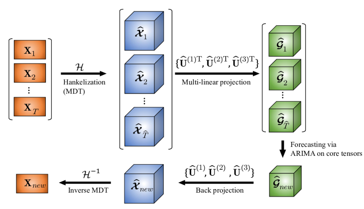
(a) BHT-ARIMA for second-order tensor TS

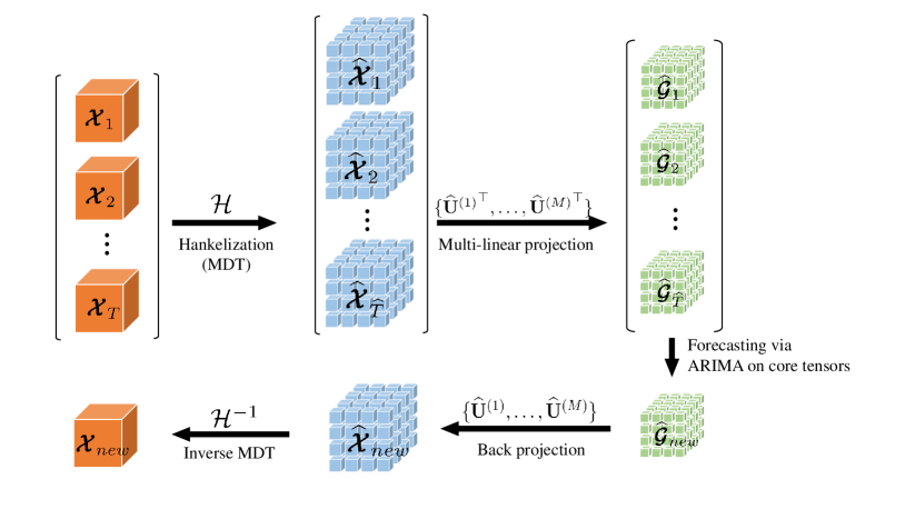
(b) BHT-ARIMA for third-order tensor TS

Figure 1: Illustration of the proposed method for prediction of multiple TS represented by a set of second/third-order tensors. Extension to higher-order tensors is straightforward.

Tensor decomposition-based methods

These tensor approaches preserve the structure of high-order data and can handle multiple TS simultaneously (?; ?; ?; ?; ?). The closest related work is the MOAR which collectively integrates Tucker decomposition with AR for high-order TSF (?):

$$\mathop{\min}_{\{{\mathbf{U}}^{(i)}\},\{\alpha_{i}\}} \sum_{t=2}^{{T}}\ \Big{\|}\Big{(}{{\boldsymbol{\mathcal{X}}}_{t}}-\sum_{i=1}^{p}\alpha_{i}{{\boldsymbol{\mathcal{X}}}_{t-i}}\Big{)}\prod_{n=1}^{N}\times_{n}{\mathbf{U}}{{}^{(n)}}^{\top}\Big{\|}_{F}^{2}$$ (4)

$$\text{s.t.}\ \ {\mathbf{U}}{{}^{(n)}}^{\top}{\mathbf{U}}{{}^{(n)}}=\mathbf{I},n=1,\ldots,N,$$

where $\mathbf{I}$ is an identity matrix and the core tensors are formulated in Tucker model and implicitly used to train the AR model. Our BHT-ARIMA differs from this closest related MOAR in three key aspects:1) BHT-ARIMA utilizes the BHT as input which can be better estimated than original data, especially for shorter univariate TS. This will be also verified by using BHT to improve MOAR; 2) BHT-ARIMA explicitly uses low-rank core tensors to train its model while MOAR does not directly use them. Since the core tensors are smaller and can better capture the intrinsic temporal correlations than original TS data. BHT-ARIMA can improve computational speed and forecasting accuracy than MOAR; 3) BHT-ARIMA removes non-stationarity of TS data by using differencing technique which is not considered in MOAR.

Besides, some works integrate decomposition with neural networks (?; ?; ?), like tensor-train decomposition with recurrent neural network (TTRNN) (?) can achieve promising results for higher-order non-linear TS. However, these tensor methods are not applicable for short univariate TS which cannot be presented as high-order tensors naturally.

MDT for multiple TS

Hankelization is an effective way to transform lower-order data to higher-order tensors. MDT is a multi-way extension of Hankelization and show good results in tensor completion (?; ?). It combines multi-linear duplication and multi-way folding operations. By denoting $\widehat{\boldsymbol{\mathcal{X}}}\in\mathbb{R}^{J_{1}\times J_{2}\cdots\times J_{M}}$ as the block Hankel tensor of $\boldsymbol{\mathcal{X}}\in\mathbb{R}^{I_{1}\times I_{2}\times\cdots\times I_{N}},N<M$, the MDT for $\boldsymbol{\mathcal{X}}$ is defined by

$$\widehat{\boldsymbol{\mathcal{X}}}=\boldsymbol{\mathcal{H}}_{\boldsymbol{\tau}}(\boldsymbol{\mathcal{X}})=\text{Fold}_{(\mathbf{I},\boldsymbol{\tau})}(\boldsymbol{\mathcal{X}}\times_{1}\mathbf{S}_{1}\cdots\times_{N}\mathbf{S}_{N}),$$ (5)

where $\mathbf{S}_{n}\in\mathbb{R}^{\tau_{n}(I_{n}-\tau_{n}+1)\times I_{n}}$ is a duplication matrix and $\text{fold}_{(\mathbf{I},\boldsymbol{\tau})}:\mathbb{R}^{\tau_{1}(I_{1}-\tau_{1}+1)\times\cdots\times\tau_{N}(I_{N}-\tau_{N}+1)}$ $\rightarrow$ $\mathbb{R}^{\tau_{1}\times(I_{1}-\tau_{1}+1)\times\cdots\times\tau_{N}\times(I_{N}-\tau_{N}+1)}$ constructs a higher order block Hankel tensor $\widehat{\boldsymbol{\mathcal{X}}}$ from the input tensor ${\boldsymbol{\mathcal{X}}}$. The inverse MDT for $\widehat{\boldsymbol{\mathcal{X}}}$ is given by

$${\boldsymbol{\mathcal{X}}}=\mathcal{H}_{\boldsymbol{\tau}}^{-1}(\widehat{\boldsymbol{\mathcal{X}}})=\text{Unfold}_{(\mathbf{I},\boldsymbol{\tau})}(\widehat{\boldsymbol{\mathcal{X}}})\times_{1}\mathbf{S}_{1}^{\dagger}\cdots\times_{N}\mathbf{S}_{N}^{\dagger},$$ (6)

where $\dagger$ is the Moore-Penrose pseudo-inverse.

Proposed Block Hankel Tensor ARIMA

To effectively and efficiently address the multiple (short) TSF problem, we propose to incorporate block Hankel tensor with ARIMA (BHT-ARIMA) via low-rank Tucker decomposition. The main idea of the proposed method is illustrated in Fig. 1. It consists of three major steps.

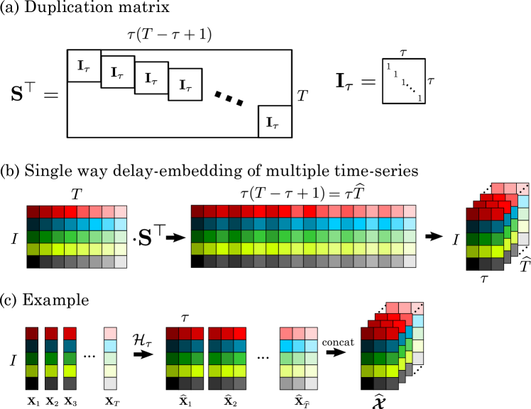
Figure 2: Illustration of applying MDT along the temporal mode of multiple TS represented as a matrix $\mathbf{X}\in\mathbb{R}^{I\times T}$. As we view the last mode $N$ ($N=2$ in this example) of multiple TS as the temporal mode, i.e., $I_{N}=T$, the last mode duplication matrix $\mathbf{S}_{N}\in\mathbb{R}^{\tau_{N}(I_{N}-\tau_{N}+1)\times I_{N}}=\mathbf{S}\in\mathbb{R}^{\tau(T-\tau+1)\times T}$. Note that $\mathbf{X}\times_{N}\mathbf{S}$ = $\mathbf{X}\mathbf{S}^{\top}$ for matrix case. Extension to multi-modes is straightforward for tensors.

Step 1: Block Hankel Tensor via MDT

In this step, we aim to employ MDT to transform multiple TS to a high-order block Hankel tensor. Let $\boldsymbol{\mathcal{X}}\in\mathbb{R}^{I_{1}\times\cdots\times I_{N}\times T}$ be the input data where each fiber is one TS and the last mode $T$ is the temporal mode. We conduct the MDT only along the temporal direction, i.e.,

$${\widehat{\boldsymbol{\mathcal{X}}}}=\mathcal{H}_{\tau}(\boldsymbol{\mathcal{X}})\in\mathbb{R}^{J_{1}\times\cdots\times J_{M}\times\widehat{T}},$$ (7)

where $J_{n}=I_{n}$ for $n=1,...,N$, $J_{M}=\tau$ and $\widehat{T}=T-\tau+1$. In this way, we get a block Hankel tensor in high-dimensional embedded space, where each frontal slice ${\widehat{\boldsymbol{\mathcal{X}}}_{t}}\in\mathbb{R}^{J_{1}\times\cdots\times J_{M}}$ contains the data points of all the TS at $t$-th time point.

Fig. 2 illustrates conducting MDT only along the temporal mode of a second-order tensor, i.e., using the duplication matrix $\mathbf{S}$ with $\tau$ to transform $\mathbf{X}\in\mathbb{R}^{I\times T}$ to a third-order block Hankel tensor $\widehat{\boldsymbol{\mathcal{X}}}\in\mathbb{R}^{I\times\tau\times{(T-\tau+1)}}$. The block Hankel tensor is assumed to be low-rank or smooth in the embedded space (?).

Remark 1:

We only apply MDT along the temporal mode because the relationship between neighbor items of multiple TS is usually not stronger than their temporal correlation. Thus, it is unnecessary to conduct MDT on all the modes which probably not be meaningful while costing more time (we empirically study it, see Fig. 6 in the Supplementary). Nevertheless, our proposed method is capable to apply MDT on more modes to get a higher-order block Hankel tensor.

In this paper, we mainly handle second-order and third-order original tensors, see more details of applying MDT on them in Appendix A.1 of Supplementary Material (Supp.).

Step 2: Tensor ARIMA with Tucker Decomposition

In this step, we generalize the classical ARIMA to tensor form and incorporate it into Tucker decomposition. Specifically, with the block Hankel tensor, we compute its order-$d$ differencing to get $\{\Delta^{d}\widehat{\boldsymbol{\mathcal{X}}}_{t}\}_{t=d}^{\widehat{T}}$. We then employ Tucker decomposition for $\{\Delta^{d}\widehat{\boldsymbol{\mathcal{X}}}_{t}\}$ by projecting it to core tensors $\{\Delta^{d}\widehat{\boldsymbol{\mathcal{G}}}_{t}\}$ using joint orthogonal factor matrices $\{\widehat{\mathbf{U}}{{}^{(m)}}\}$, i.e.,

$$\Delta^{d} {\widehat{\boldsymbol{\mathcal{G}}}_{t}}=\Delta^{d}{\widehat{\boldsymbol{\mathcal{X}}}_{t}}\times_{1}\widehat{\mathbf{U}}{{}^{(1)}}^{\top}\cdots\times_{M}\widehat{\mathbf{U}}{{}^{(M)}}^{\top}$$ (8)

$$\text{s.t.}\ \ \widehat{\mathbf{U}}{{}^{(m)}}^{\top}\widehat{\mathbf{U}}{{}^{(m)}}=\mathbf{I},m=1,\ldots,M,$$

where the projection matrices $\{\widehat{\mathbf{U}}{{}^{(m)}}\in\mathbb{R}^{J_{m}\times R_{m}}\}$ maximally preserve the temporal continuity between core tensors and the low-rank core tensors $\{{\Delta^{d}\widehat{\boldsymbol{\mathcal{G}}}_{t}}\in\mathbb{R}^{R_{1}\times\cdots\times R_{M}}\}$ represent the most important information of original Hankel tensors and reflect the intrinsic interactions between TS.

Then, it would be more promising to train a good forecasting model directly using core tensors explicitly instead of whole tensors. To retain the temporal correlations among core tensors, we generalize a $(p,d,q)$-order ARIMA model to tensor form and use it to connect the current core tensor ${\Delta^{d}\widehat{\boldsymbol{\mathcal{G}}}_{t}}$ and the previous core tensors ${\Delta^{d}\widehat{\boldsymbol{\mathcal{G}}}_{t-1}},\Delta^{d}{\widehat{\boldsymbol{\mathcal{G}}}_{t-2}},\ldots,\Delta^{d}{\widehat{\boldsymbol{\mathcal{G}}}_{t-p}}$ as follows:

$$\Delta^{d}{\widehat{\boldsymbol{\mathcal{G}}}_{t}} =\sum_{i=1}^{p}\alpha_{i}{\Delta^{d}\widehat{\boldsymbol{\mathcal{G}}}_{t-i}}-\sum_{i=1}^{q}\beta_{i}{\widehat{\boldsymbol{\mathcal{E}}}_{t-i}}+\widehat{\boldsymbol{\mathcal{E}}}_{t},$$ (9)

where the $\{\alpha_{i}\}$ and $\{\beta_{i}\}$ are the coefficients of AR and MA, respectively, and $\{\widehat{\boldsymbol{\mathcal{E}}}_{t-i}\}$ are the random errors of past $q$ observations. In model (9), $\widehat{\boldsymbol{\mathcal{E}}}_{t}$ is the forecast error at the current time point, which should be minimized to optimal zero. We thus can derive the following objective function:

$$\mathop{\min}_{\{\widehat{\boldsymbol{\mathcal{G}}}_{t},\widehat{\mathbf{U}}{{}^{(m)}},\widehat{\boldsymbol{\mathcal{E}}}_{t-i},\alpha_{i},\beta_{i}\}}\sum_{t=s+1}^{\widehat{T}}\Bigg{(}\frac{1}{2}\Big{\|}{\Delta^{d}\widehat{\boldsymbol{\mathcal{G}}}_{t}}-\sum_{i=1}^{p}\alpha_{i}{\Delta^{d}\widehat{\boldsymbol{\mathcal{G}}}_{t-i}}+\sum_{i=1}^{q}\beta_{i}{\widehat{\boldsymbol{\mathcal{E}}}_{t-i}}\Big{\|}_{F}^{2}$$ (10)

$$\ \ \ \ \ \ \ \ \ \ \ \ \ \ \ \ +\frac{1}{2}\Big{\|}{\Delta^{d}\widehat{\boldsymbol{\mathcal{G}}}_{t}}-{\Delta^{d}\widehat{\boldsymbol{\mathcal{X}}}_{t}}\times_{1}\widehat{\mathbf{U}}{{}^{(1)}}^{\top}\cdots\times_{M}\widehat{\mathbf{U}}{{}^{(M)}}^{\top}\Big{\|}_{F}^{2}\Bigg{)}\ \$$

$$\ \ \ \ \ \ \ \ \ \ \ \ \ \ \ \ \ \ \ \ \text{s.t.}\ \ \widehat{\mathbf{U}}{{}^{(m)}}^{\top}\widehat{\mathbf{U}}{{}^{(m)}}=\mathbf{I},m=1,\ldots,M,$$

where $s=p+d+q$ is the sum of ARIMA orders, and is also the minimum input length of each TS. Next, we solve this problem using augmented Lagrangian methods. To facilitate the derivation of (10), we reformulate the optimization problem by unfolding each tensor variable along mode-$m$:

$$\mathop{\min}_{\{{\widehat{\mathbf{G}}^{(m)}_{t}},{\widehat{\mathbf{E}}^{(m)}_{{t-i}}},\widehat{\mathbf{U}}{{}^{(m)}},\alpha_{i},\beta_{i}\}}\sum_{t=s+1}^{\widehat{T}}\sum_{m=1}^{M}\Bigg{(}\frac{1}{2}\Big{\|}\Delta^{d}{\widehat{\mathbf{G}}^{(m)}_{t}}-\sum_{i=1}^{p}\alpha_{i}\Delta^{d}{\widehat{\mathbf{G}}^{(m)}_{{t-i}}}$$ (11)

$$\ \ \ \ \ \ \ \ +\sum_{i=1}^{q}\beta_{i}{\widehat{\mathbf{E}}^{(m)}_{{t-i}}}\Big{\|}_{F}^{2}+\frac{1}{2}\Big{\|}\Delta^{d}{\widehat{\mathbf{G}}^{(m)}_{t}}-\widehat{\mathbf{U}}{{}^{(m)}}^{\top}{\widehat{\mathbf{X}}^{(m)}_{t}}\widehat{\mathbf{U}}{{}^{(-m)}}^{\top}\Big{\|}_{F}^{2}\Bigg{)}$$

$$\ \ \ \ \ \ \ \ \ \ \ \ \ \text{s.t.}\ \ \widehat{\mathbf{U}}{{}^{(m)}}^{\top}\widehat{\mathbf{U}}{{}^{(m)}}=\mathbf{I},m=1,\ldots,M,$$

where $\widehat{\mathbf{U}}{{}^{(-m)}}=\widehat{\mathbf{U}}{{}^{(M)}}^{\top}\otimes\cdots\widehat{\mathbf{U}}{{}^{(m+1)}}^{\top}\otimes\widehat{\mathbf{U}}{{}^{(m-1)}}^{\top}\otimes\cdots\widehat{\mathbf{U}}{{}^{(1)}}^{\top}\in\mathbb{R}^{\prod_{j\neq m}R_{j}\times\prod_{j\neq m}I_{j}}$. In the following, we can update each target variable using closed-form solutions .

Update $\widehat{\mathbf{G}}^{(m)}_{t}$

Equation (11) with respect to $\Delta^{d}\widehat{\mathbf{G}}^{(m)}_{t}$ is:

$$\begin{aligned} \mathop{\min}_{\{\widehat{\mathbf{G}}^{(m)}_{t}\}}\sum_{t=s+1}^{\widehat{T}}\sum_{m=1}^{M}&\Bigg{(}\frac{1}{2}\Big{\|}\Delta^{d}{\widehat{\mathbf{G}}^{(m)}_{t}}-\sum_{i=1}^{p}\alpha_{i}\Delta^{d}{\widehat{\mathbf{G}}^{(m)}_{{t-i}}}+\sum_{i=1}^{q}\beta_{i}{\widehat{\mathbf{E}}^{(m)}_{{t-i}}}\Big{\|}_{F}^{2}\\ &+\frac{1}{2}\Big{\|}\Delta^{d}{\widehat{\mathbf{G}}^{(m)}_{t}}-\widehat{\mathbf{U}}{{}^{(m)}}^{\top}{\widehat{\mathbf{X}}^{(m)}_{t}}\widehat{\mathbf{U}}{{}^{(-m)}}^{\top}\Big{\|}_{F}^{2}\Bigg{)}.\end{aligned}\$$ (12)

Computing the partial derivation of this cost function with respect to ${\widehat{\mathbf{G}}^{(m)}_{t}}$ and equalize it to zero, we update $\widehat{\mathbf{G}}^{(m)}_{t}$ by:

$$\Delta^{d}\widehat{\mathbf{G}}^{(m)}_{t} =\frac{1}{2}\Big{(}\widehat{\mathbf{U}}{{}^{(m)}}^{\top}{\widehat{\mathbf{X}}^{(m)}_{t}}\widehat{\mathbf{U}}{{}^{(-m)}}^{\top}$$ (13)

$$+\sum_{i=1}^{p}\alpha_{i}\Delta^{d}{\widehat{\mathbf{G}}^{(m)}_{{t-i}}}-\sum_{i=1}^{q}\beta_{i}{\widehat{\mathbf{E}}^{(m)}_{{t-i}}}\Big{)}.$$

Update $\widehat{\mathbf{U}}{{}^{(m)}}$

Equation (11) with respect to $\widehat{\mathbf{U}}{{}^{(m)}}$ is:

$$\mathop{\min}_{\{\widehat{\mathbf{U}}{{}^{(m)}}\}}\sum_{t=s+1}^{\widehat{T}}\sum_{m=1}^{M} \frac{1}{2}\Big{\|}\Delta^{d}{\widehat{\mathbf{G}}^{(m)}_{t}}-\widehat{\mathbf{U}}{{}^{(m)}}^{\top}{\widehat{\mathbf{X}}^{(m)}_{t}}\widehat{\mathbf{U}}{{}^{(-m)}}^{\top}\Big{\|}_{F}^{2}$$ (14)

$$\text{s.t.}\ \ \widehat{\mathbf{U}}{{}^{(m)}}^{\top}\widehat{\mathbf{U}}{{}^{(m)}}=\mathbf{I},m=1,\ldots,M.$$

The minimization of (14) over $\widehat{\mathbf{U}}{{}^{(m)}}$ with orthonormal columns is equivalent to the maximization of the well-known orthogonality Procrustes problem (?), whose global optimal solution is,

$$\widehat{\mathbf{U}}{{}^{(m)}}=\widehat{\mathbf{U}^{*}}{{}^{(m)}}(\widehat{\mathbf{V}^{*}}{{}^{(m)}})^{\top},$$ (15)

where $\widehat{\mathbf{U}^{*}}{{}^{(m)}}$ and $\widehat{\mathbf{V}^{*}}{{}^{(m)}}$ are the left and right singular vectors of SVD of $\sum_{t=s+1}^{\widehat{T}}{\widehat{\mathbf{X}}^{(m)}_{t}}\widehat{\mathbf{U}}{{}^{(-m)}}^{\top}\Delta^{d}{\widehat{\mathbf{G}}{{}^{(m)}_{t}}}^{\top}$, respectively.

Discussion 1: Relaxed-orthogonality

We empirically explored the effect of relaxing the full-orthogonality in (14) by removing the orthogonal constraints along the last mode (viewed as the temporal mode of each $\widehat{\boldsymbol{\mathcal{X}}}_{t}$ in the embedded space). This strategy probably relaxes the heavy constraints on temporal smoothness and thus would make the proposed model more flexible and robust to variability of parameters, observed from our experimental results. We relax the last mode $\widehat{\mathbf{U}}^{(M)}$ without orthogonality constraint, and then compute the partial derivation of Eq. (14) with respect to $\widehat{\mathbf{U}}^{(M)}$ and equalize it to zero. Thus, we can update it by

$$\widehat{\mathbf{U}}{{}^{(M)}}= \Big{(}\sum_{t=s+1}^{\widehat{T}}{\widehat{\mathbf{X}}^{(M)}_{t}}\widehat{\mathbf{U}}{{}^{(-M)}}^{\dagger}({\widehat{\mathbf{X}}^{(M)}_{t}}\widehat{\mathbf{U}}{{}^{(-M)}}^{\dagger})^{\top}\Big{)}^{-1}$$ (16)

$$\Big{(}\sum_{t=s+1}^{\widehat{T}}{\widehat{\mathbf{X}}^{(M)}_{t}}\widehat{\mathbf{U}}{{}^{(-M)}}^{\dagger}\Delta^{d}{\widehat{\mathbf{G}}{{}^{(M)}_{t}}}^{\top}\Big{)}.$$

Update $\widehat{\mathbf{E}}^{(m)}_{{t-i}}$

Equation (11) with respect to $\widehat{\mathbf{E}}^{(m)}_{{t-i}}$ is:

$$\mathop{\min}_{\{\widehat{\mathbf{E}}^{(m)}_{{t-i}}\}}\sum_{t=s+1}^{\widehat{T}}\sum_{m=1}^{M}\frac{1}{2}\Big{\|}\Delta^{d}{\widehat{\mathbf{G}}^{(m)}_{t}}-\sum_{i=1}^{p}\alpha_{i}\Delta^{d}{\widehat{\mathbf{G}}^{(m)}_{{t-i}}}+\sum_{i=1}^{q}\beta_{i}{\widehat{\mathbf{E}}^{(m)}_{{t-i}}}\Big{\|}_{F}^{2}.$$ (17)

Computing the partial derivation of Eq. (17) with respect to $\widehat{\mathbf{E}}{{}^{(m)}_{{t-i}}}$ and equalize it to zero, we can update $\widehat{\mathbf{E}}{{}^{(m)}_{{t-i}}}$ by

$$\widehat{\mathbf{E}}{{}^{(m)}_{{t-i}}}=\frac{\sum_{t=s+1}^{\widehat{T}}\Big{(}\Delta^{d}{\widehat{\mathbf{G}}^{(m)}_{t}}-\sum_{i=1}^{p}\alpha_{i}\Delta^{d}{\widehat{\mathbf{G}}^{(m)}_{{t-i}}}+\sum_{j\neq i}^{q}\beta_{j}\widehat{\mathbf{E}}{{}^{(m)}_{{t-j}}}\Big{)}}{(s+1-\widehat{T})\beta_{i}}.$$ (18)

Update $\{\alpha_{i}\},\{\beta_{i}\}$

Regarding the coefficient parameters $\{\alpha_{i}\}_{i=1}^{p},\{\beta_{i}\}_{i=1}^{q}$ of AR and MA respectively in the objective function (11), we follow the classical ARIMA based on Yule-Walker method to estimate them. We generalize a least squares modified Yule-Walker technique to support tensorial data and then estimate the $\{\alpha_{i}\}_{i=1}^{p}$ from the core tensors. Then, we estimate the $\{\beta_{i}\}_{i=1}^{q}$ from the residual time series.

Algorithm 1 TSF using BHT-ARIMA

1:  Input: A time series data $\boldsymbol{\mathcal{X}}\in\mathbb{R}^{I_{1}\times\cdots\times I_{N}\times T}$, $(p,d,q)$, $\tau$, maximum iteration $K$, and stop criteria tol.

2:  Step 1: Block Hankel Tensor via MDT

3:  Use MDT to transform the original tensor as a block Hankel tensor: ${\widehat{\boldsymbol{\mathcal{X}}}}=\mathcal{H}_{\tau}(\boldsymbol{\mathcal{X}})\in\mathbb{R}^{J_{1}\times\cdots\times J_{M}\times\widehat{T}}$, where each frontal slice ${\widehat{\boldsymbol{\mathcal{X}}}_{t}}\in\mathbb{R}^{J_{1}\times\cdots\times J_{M}}$ refers to all the time series at $t$-th time point.

4:  Set values for $\{R_{m}\}_{m=1}^{M}$ and initialize $\{\widehat{\mathbf{U}}{{}^{(m)}}\}_{m=1}^{M}$ randomly.

5:  Step 2: Tensor ARIMA with Tucker decomposition.

6:  Conduct order-$d$ differencing for $\{{\widehat{\boldsymbol{\mathcal{X}}}_{t}}\}_{t=1}^{\widehat{T}}$ and get $\{\Delta^{d}{\widehat{\boldsymbol{\mathcal{X}}}_{t}}\}_{t=d+1}^{\widehat{T}}$

7:  Initialize $\{\{\widehat{\boldsymbol{\mathcal{E}}}_{{t-i}}\in\mathbb{R}^{R_{1}\times\cdots\times R_{M}}\}_{i=1}^{q}\}_{i=s+1}^{\widehat{T}}$ randomly.

8:  for $k=1,...,K$

9:   Compute all the latent low-dimensional core tensors  $\{\Delta^{d}{\widehat{\boldsymbol{\mathcal{G}}}_{t}}=\Delta^{d}{\widehat{\boldsymbol{\mathcal{X}}}_{t}}\times_{1}\widehat{\mathbf{U}}{{}^{(1)}}^{\top}\cdots\times_{M}\widehat{\mathbf{U}}{{}^{(M)}}^{\top}\}_{t=1}^{\widehat{T}}$;

10:   Estimate coefficients $\{\alpha_{i}\}_{i=1}^{p},\{\beta_{i}\}_{i=1}^{q}$ of AR and MA       based on Yule-Walker equations based on $\{\Delta^{d}{\widehat{\boldsymbol{\mathcal{G}}}_{t}}\}_{t=d+1}^{\widehat{T}}$

11:   for $n=1,...,M$

12:    Update $\Delta^{d}{\widehat{\mathbf{G}}^{(m)}_{t}}$ by (13) and get $\Delta^{d}{\widehat{\boldsymbol{\mathcal{G}}}_{t}}=\text{Fold}\Big{(}\Delta^{d}{\widehat{\mathbf{G}}^{(m)}_{t}}\Big{)}$

13:    Update $\widehat{\mathbf{U}}{{}^{(m)}}$ by (15)

14:    If applying relaxed-orthogonality, update $\widehat{\mathbf{U}}{{}^{(M)}}$ by (16).

15:    for  $i=1,...,q$

16:     Update $\widehat{\mathbf{E}}^{(n)}_{{t-i}}$ by (18) and update $\widehat{\boldsymbol{\mathcal{E}}}_{{t-i}}$ by $\text{Fold}\Big{(}\widehat{\mathbf{E}}^{(m)}_{{t-i}}\Big{)}$

17:   Convergence checking: if $\frac{\sum_{m=1}^{M}||\widehat{\mathbf{U}}{{}^{(m)}}^{k+1}-\widehat{\mathbf{U}}{{}^{(m)}}^{k}||_{F}^{2}}{\sum_{m=1}^{M}||\widehat{\mathbf{U}}{{}^{(m)}}^{k+1}||_{F}^{2}}<tol$, break; otherwise, continue.

18:  Step 3: Forecasting

19:  Compute new observation by (19) to get $\Delta^{d}{\widehat{\boldsymbol{\mathcal{G}}}_{t+1}}$ and then compute $\Delta^{d}{\widehat{\boldsymbol{\mathcal{X}}}_{\widehat{T}+1}}=\Delta^{d}{\widehat{\boldsymbol{\mathcal{G}}}_{{t}+1}}\prod_{m=1}^{M}\times_{m}\widehat{\mathbf{U}}{{}^{(m)}}$.

20:  Conduct inverse differencing for $\Delta^{d}{\widehat{\boldsymbol{\mathcal{X}}}_{\widehat{T}+1}}$ and get ${\widehat{\boldsymbol{\mathcal{X}}}_{\widehat{T}+1}}$.

21:  Conduct inverse MDT: ${{\boldsymbol{\mathcal{X}}}_{T+1}}=\mathcal{H}_{\tau}^{-1}({{\widehat{\boldsymbol{\mathcal{X}}}}_{\widehat{T}+1}})$

22:  Output: ${{\boldsymbol{\mathcal{X}}}_{T+1}}$, $\{\widehat{\mathbf{U}}{{}^{(1)}},\ldots,\widehat{\mathbf{U}}{{}^{(m)}},\ldots,\widehat{\mathbf{U}}{{}^{(M)}}\}$.

Step 3: Forecasting ${{\boldsymbol{\mathcal{X}}}_{T+1}}$

Finally, we apply the learned model to get a new $\Delta^{d}{\widehat{\boldsymbol{\mathcal{G}}}_{\widehat{T}+1}}$:

$$\Delta^{d}{\widehat{\boldsymbol{\mathcal{G}}}_{\widehat{T}+1}}=\sum_{i=1}^{p}\alpha_{i}\Delta^{d}{\widehat{\boldsymbol{\mathcal{G}}}_{\widehat{T}-i}}-\sum_{i=1}^{q}\beta_{i}{\widehat{\boldsymbol{\mathcal{E}}}_{\widehat{T}-i}}.$$ (19)

After obtaining $\Delta^{d}{\widehat{\boldsymbol{\mathcal{G}}}_{\widehat{T}+1}}$, we reconstruct a new tensor by Tucker model with optimized factor matrices: $\Delta^{d}{\widehat{\boldsymbol{\mathcal{X}}}_{\widehat{T}+1}}=\Delta^{d}{\widehat{\boldsymbol{\mathcal{G}}}_{{t}+1}}\prod_{m=1}^{M}\times_{m}\widehat{\mathbf{U}}{{}^{(m)}}$. We then conduct inverse order-$d$ differencing for $\Delta^{d}{\widehat{\boldsymbol{\mathcal{X}}}_{\widehat{T}+1}}$ and get ${\widehat{\boldsymbol{\mathcal{X}}}_{\widehat{T}+1}}\in\mathbb{R}^{J_{1}\times\cdots\times J_{M}\times{(\widehat{T}+1)}}$ in the embedded space. Finally, we apply inverse MDT to get ${{\boldsymbol{\mathcal{X}}}_{T+1}}=\mathcal{H}_{\tau}^{-1}({\widehat{\boldsymbol{\mathcal{X}}}_{\widehat{T}+1}})\in\mathbb{R}^{I_{1}\times\cdots\times I_{N}\times{(T+1)}}$ to get the predicted values at the $T+1$-th time point for all TS simultaneously. Furthermore, we could do long-term forecasting by using prior foretasted values in last steps. Although this way may lead to error accumulation to some degree, it becomes more practical for real-world applications (?).

Remark 2:

We explicitly use the compressed core tensors to train the model including parameters estimation. That is different from existing tensor methods like MOAR which implicitly use the core tensors to train their models. In this manner, we not only reduce the computational cost since the size of core tensors $\{\widehat{\boldsymbol{\mathcal{G}}}_{t}\}$ are much smaller than whole tensors $\{\widehat{\boldsymbol{\mathcal{X}}}_{t}\}$ based on the low-rank assumption in the embedded space, but also improve the forecasting accuracy by utilizing the mutual correlations among multiple TS in the model building process.

Finally, we summarize the proposed BHT-ARIMA in Algorithm 1 and further evaluate it in the following section.

Experiments

Due to limited space, we present the detailed experimental setup and parameter analysis with figures in the Supp..

Experimental Setup

Datasets

We evaluate the proposed BHT-ARIMA by conducting experiments on five real-world datasets, including: i)Three publicly available datasets: Traffic is originally collected from California department of transportation and describes the road occupy rate of Los Angeles County highway network. We here use the same subset in (?) which selects 228 sensors randomly and we aggregate it to daily interval for each TS with 80 days data points. Electricity records 321 clients’ hourly electricity consumption (?). We merge the every 24 time points to obtain a daily interval TS dataset with size $321\times 1096$. Smoke Video records the Smoke from the chimney of a factory taken in Hokkaido in 2007. We sample and resize the images to obtain a third-order TS dataset of size 36$\times$64$\times$100;
ii)Two industrial datasets from the supply chain of Huawei: PC sales has 105 weekly sales records of 9 personal computers from 2017 to 2019; Raw materials includes 2246 material items of making a product, each item has 24 monthly demand quantities. We illustrate these datasets in Fig. $1$ and $2$ in the Supp..

Compared methods

We compared nine competing methods: i) the classical ARIMA, Vector AR (VAR) and XGBoost (?); ii) the two popular industrial forecasting methods: Facebook-Prophet, and Amazon-DeepAR (?); iii) Neural network based methods: TTRNN (?) and Gated Recurrent Units (GRU) (?); iv) the two matrix/tensor-based methods: TRMF (?), and MOAR; In addition, we combine MDT with MOAR by using our obtained block Hankel tensor as the input of MOAR to get BHT+MOAR to evaluate the effectiveness of MDT together with tensor decomposition.

Parameter settings

All datasets are split into training sets (90$\%$) and testing sets (10$\%$). We conduct grid search over parameters for each model and dataset (See Appendix B.1 of Supp. in detail). For our BHT-ARIMA, we will show its analysis of parameters in the following. We measure the forecasting accuracy using the widely used Normalized Root Mean Square Error (NRMSE) metric.

Analysis of Parameters and Convergence

We here not only analyze the parameter sensitivity of BHT-ARIMA, but also study the effects of BHT-ARIMA with relaxed-orthogonality and MDT on all modes by testing on the Raw materials and Smoke video datasets, respectively.

Sensitivity Analysis of Parameters $\tau$, $\{R_{m}\}$ and $(p,d,q)$

Fig. $3$, $4$ and $5$ in the Supp. show the forecasting results using BHT-ARIMA with full-orthogonality (FO) versus (vs.) relaxed-orthogonality (RO) with different values of the parameters $\tau$, $\{R_{m}\}$ and $(p,d,q)$, respectively. Overall, BHT-ARIMA with RO is less sensitive and can achieve even slightly better forecasting accuracy than that with FO. Particularly, with very small $\tau$ (e.g. 1,2,5) and when the last mode rank $R_{M}=\tau$ (that maximally preserves the temporal dependencies among core tensors), BHT-ARIMA with FO can achieve better (similar) accuracy than that with RO. With the same differencing order $d$, the performance of BHT-ARIMA is relatively sensitive to too large $p$. Besides, the time cost of BHT-ARIMA with RO is larger than that of with FO due to the cost of computing Eq. (16) is larger than that of Eq. (15).

In short, we do not need to carefully tune the parameters for BHT-ARIMA while we usually can obtain better results by setting smaller values such as { $\tau={2-4}$, $R_{M}=\tau$ and small $(p={1-5},d={1},q={1})$}. Moreover, the Tucker-rank can be estimated automatically (?; ?).

Effect of applying MDT on all modes / temporal mode

As discussed in Remark 1 about why we apply MDT only along the temporal mode, we here verify it by testing on the Smoke video. As shown in Fig. $6$ in the Supp.: both types of applying MDT obtain similar forecasting accuracy while using MDT on all the modes costs more time due to computing higher-order tensors. This conclusion is also applicable for the cases of BHT-ARIMA with RO. These results support our assumption that these TS items usually do not have strong neighborhood relationships so it is unnecessary to applying MDT on other modes besides the temporal mode.

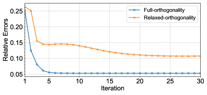
Figure 3: Convergence curves of BHT-ARIMA on the Raw materials dataset.

Convergence and maximum iteration $K$

We study the convergence of BHT-ARIMA in terms of the relative error of projection matrices $\frac{\sum_{m=1}^{M}||\widehat{\mathbf{U}}{{}^{(m)}}^{k+1}-\widehat{\mathbf{U}}{{}^{(m)}}^{k}||_{F}^{2}}{\sum_{m=1}^{M}||\widehat{\mathbf{U}}{{}^{(m)}}^{k+1}||_{F}^{2}}$. Fig. 3 shows that both BHT-ARIMA with FO and RO converge quickly while the FO version converges more smoothly and faster within 10 iterations. Furthermore, setting maximum iteration $K>5$ is enough to get a sufficient forecasting accuracy, as shown in Fig. $7(b)$ in the Supp.. In this paper, we set $K=10$ for BHT-ARIMA for all the tests.

Forecasting Accuracy Comparison

We report the average forecasting results of 10 runs in Tables 1, 2 and 3, where we highlight the best results in bold font and underline the second best results. Note that BHT-ARIMA used in the following comparisons is the full-orthogonality version.

Table 1: Forecasting results comparison on the Electricity and Traffic (measured in NRMSE).

	Electricity1096 ( $\times 10^{-2}$)	Electricity40 ($\times 10^{-2}$)	Traffic80 ($\times 10^{-3}$)	Traffic40 ($\times 10^{-3}$)
ARIMA	1.316	10.091	3.194	6.097
VAR	12.850	1.834	6.649	1.526
XGBoost	1.839	2.724	4.900	3.727
Prophet	13.799	5.948	4.343	1.992
DeepAR	4.742	4.857	8.178	5.358
TTRNN	2.686	3.565	5.723	3.432
GRU	1.574	1.545	1.371	0.782
TRMF	6.221	2.713	5.800	2.340
MOAR	4.731	7.677	10.689	12.200
BHT+MOAR	3.787	4.050	4.920	4.464
BHT-ARIMA	1.114	1.456	0.599	0.493

Table 2: Forecasting results comparison on the PC sales and Raw materials (measured in NRMSE).

	PC sales ($9\times 105$)	Raw materials$\_$I ($1533\times 24$)	Raw materials$\_$II ($2246\times 24$)
ARIMA	0.604	3.217	3.836
VAR	0.690	3. 387	4.033
XGBoost	0.618	3.834	4.231
Prophet	0.593	2.984	3.734
DeepAR	0.689	3.158	4.476
TTRNN	0.616	2.828	3.373
GRU	0.524	2.592	3.250
TRMF	0.689	3.167	4.362
MOAR	0.689	2.207	2.635
BHT+MOAR	0.683	2.114	2.525
BHT-ARIMA	0.490	1.558	1.856

Table 3: Computational cost (seconds) vs. SOTA algorithms on all five real-world TS datasets.

Time(s)	Electricity1096 $(321\times 1096)$	Electricity40 $(321\times 40)$	Traffic80 $(228\times 80)$	Traffic40 $(228\times 40)$	PC sales $(9\times 105)$	Raw materials$\_$I $(1533\times 24)$	Raw materials$\_$II $(2246\times 24)$	Smoke Video $(32\times 64\times 100)$
ARIMA	3322.62	327.60	453.63	382.32	13.01	1151.35	2067.48	1340.20
VAR	68.96	2.042	4.19	0.92	0.27	11.32	25.51	69.63
XGBoost	108.02	26.07	23.28	6.94	8.87	148.22	159.33	178.86
Prophet	2160.33	1304.07	1241.43	335.23	53.31	434.15	853.23	13813.21
DeepAR	175.56	171.17	119.02	112.04	78.43	136.80	286.66	106.65
TTRNN	165.84	104.38	88.77	95.47	22.83	25.49	28.05	27.82
GRU	4383.81	1077.09	1104.17	858.03	93.34	3353.43	3534.96	3142.46
TRMF	16.03	0.57	1.90	1.22	1.46	0.27	0.28	0.77
MOAR	28.96	10.21	6.75	5.78	1.68	566.19	1612.52	7.26
BHT+MOAR	42.86	12.28	8.28	5.93	1.70	865.91	1700.49	10.95
BHT-ARIMA	23.24	0.89	1.28	0.58	1.41	0.91	1.13	3.67

Forecasting results of longer vs. shorter TS

To evaluate the capability of BHT-ARIMA for longer vs. shorter TS, we sample the first 40 time points of the Traffic dataset and thus get shorter Traffic40 ($228\times 40$) and denote original whole set as Traffic80. For the Electricity, we sample the first 40 time points and get Electricity40 ($321\times 40$), and the whole one is denoted as Electricity1096. The results are reported in Table 1: BHT-ARIMA outperforms all the existing competing methods in all the cases. Especially for shorter TS, BHT-ARIMA shows more advantage with 54.5$\%$ improvement on average on the Traffic data than that of on the Electricity (7.9$\%$ improvement on average). GRU and ARIMA share the second best results. Note that BHT+MOAR performs consistently better than MOAR in all cases, which verifies the effectiveness of applying MDT together with tensor decomposition.

Forecasting results of industrial TS datasets

In practice, industrial datasets are more complex with random irregular patterns and larger variance compared to these public datasets. As reported in the Table 2: 1) For PC sales with only nine TS items, BHT-ARIMA outperforms the second best performing method GRU by 6.5$\%$ on average; 2) For Raw materials dataset which has shorter length (24 months) than PC sales (105 weeks) while has much larger number of items (2246), we remove the items with missing values and get 1553 items namely Raw materials$\_$I while the original one named as Raw materials$\_$II. In such scenarios, BHT + MOAR and GRU perform better than other existing methods, although their results are much worse than our BHT-ARIMA. These results further confirm the effectiveness of MDT together with tensor decomposition and also verified the improvement of explicitly using the core tensors to train our ARIMA model.

Forecasting results of Smoke video

We further evaluate the performance of BHT-ARIMA on higher-order TS data using the Smoke video with $10\%-90\%$ training set. Fig. 4 shows that BHT-ARIMA consistently forecasts the next video frame with smaller errors using even $10\%$ training data (10 frames) where ARIMA, MOAR and other methods fail to keep their performance. Moreover, although ARIMA can achieve slightly better accuracy than ours with more than $50\%$ training data, it surfers from extremely larger computational cost and memory requirements because like other linear models who cannot directly handle tensor TS data and need to reshape them into vectors.

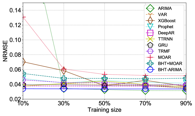
Figure 4: Forecasting accuracy comparison on the Smoke video. In the case of using $10\%$ training size, the NRMSE of ARIMA is too large (0.277) so we truncate its curve there.

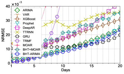
(a) Traffic80

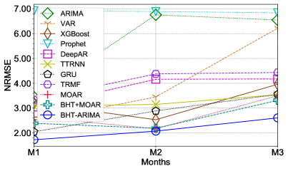
(b) Raw materials$\_$II

Figure 5: Long-term forecasting results for the Traffic and Raw materials (truncate curves with too large NRMSE).

Long-term Forecasting Comparison

Fig. 5 shows the comparison of long-term forecasting results, which further confirm the promising performance of BHT-ARIMA. Forecasting more steps, the errors of all the methods increase in general while BHT-ARIMA consistently keeps its best performance on the whole, especially on the shorter Raw materials dataset. Note that GRU slightly outperforms our method after 15 steps on Traffic80 dataset, but it requires near 900 times computational cost than ours.

Time Cost Comparison

We report the average time cost of forecasting in Table 3. Although TRMF is slightly slower than VAR in a few cases, it is the fastest algorithm on the whole due to its core parts are implemented by C programming. BHT-ARIMA is the second fastest method while our implementations are not optimized for efficiency as our focus here is accuracy. MOAR is slower than ours mainly because it does not directly use the low-dimensional core tensors for training. ARIMA and GRU are the second best performing algorithms in a few cases, but they are the most slowest methods (more than 500 times slower than BHT-ARIMA on average).

Conclusions

In this paper, we proposed a novel BHT-ARIMA for multiple (short) TSF. BHT-ARIMA tactically utilizes the unique strengths of smart tensorization via MDT, tensor ARIMA, and low-rank Tucker decomposition in a unified model. With low-rank Hankel tensor in embedded space by MDT Hankelization along the temporal mode, we further obtain the compressed core tensors using Tucker decomposition. The core tensors capture the intrinsic correlations among multiple TS and are explicitly used to train the tensor ARIMA model. BHT-ARIMA can improve forecasting accuracy and computational speed, especially for multiple short TS. We also empirically studied its robustness to various parameters by comparing it with its relaxed-orthogonality version. Experiments conducted on five real-world TS datasets demonstrate that BHT-ARIMA outperforms the SOTA methods with significant improvement.

References

- [Agarwal et al. 2018] Agarwal, A.; Amjad, M. J.; Shah, D.; and Shen, D. 2018. Model agnostic time series analysis via matrix estimation. POMACS 2(3):40.
- [Bhanu et al. 2018] Bhanu, M.; Priya, S.; Dandapat, S. K.; Chandra, J.; and Mendes-Moreira, J. 2018. Forecasting traffic flow in big cities using modified Tucker decomposition. In ADMA, 119–128. Springer.
- [Box and Jenkins 1968] Box, G. E., and Jenkins, G. M. 1968. Some recent advances in forecasting and control. Journal of the Royal Statistical Society. Series C (Applied Statistics) 17(2):91–109.
- [Chen and Guestrin 2016] Chen, T., and Guestrin, C. 2016. Xgboost: A scalable tree boosting system. In ACM SIGKDD, 785–794. ACM.
- [Chen et al. 2018] Chen, P.; Liu, S.; Shi, C.; Hooi, B.; Wang, B.; and Cheng, X. 2018. NeuCast: seasonal neural forecast of power grid time series. In IJCAI, 3315–3321. AAAI Press.
- [Cho et al. 2014] Cho, K.; Van Merriënboer, B.; Gulcehre, C.; Bahdanau, D.; Bougares, F.; Schwenk, H.; and Bengio, Y. 2014. Learning phrase representations using rnn encoder-decoder for statistical machine translation. arXiv preprint arXiv:1406.1078.
- [Cichocki et al. 2016] Cichocki, A.; Lee, N.; Oseledets, I.; Phan, A.-H.; Zhao, Q.; Mandic, D. P.; et al. 2016. Tensor networks for dimensionality reduction and large-scale optimization: Part 1 low-rank tensor decompositions. Found. Trends® Mach. Learn. 9(4-5):249–429.
- [de Araujo, Ribeiro, and Faloutsos 2017] de Araujo, M. R.; Ribeiro, P. M. P.; and Faloutsos, C. 2017. Tensorcast: Forecasting with context using coupled tensors. In ICDM, 71–80. IEEE.
- [Ding, Qi, and Wei 2015] Ding, W.; Qi, L.; and Wei, Y. 2015. Fast Hankel tensor–vector product and its application to exponential data fitting. Numer. Linear Algebra Appl. 22(5):814–832.
- [Dunlavy, Kolda, and Acar 2011] Dunlavy, D. M.; Kolda, T. G.; and Acar, E. 2011. Temporal link prediction using matrix and tensor factorizations. ACM Trans. Knowl. Discov. Data 5(2):10.
- [Faloutsos et al. 2018] Faloutsos, C.; Gasthaus, J.; Januschowski, T.; and Wang, Y. 2018. Forecasting big time series: old and new. Proceedings of the VLDB Endowment 11(12):2102–2105.
- [Faloutsos et al. 2019] Faloutsos, C.; Flunkert, V.; Gasthaus, J.; Januschowski, T.; and Wang, Y. 2019. Forecasting big time series: Theory and practice. In ACM SIGKDD, 3209–3210. ACM.
- [Fanaee-T and Gama 2016] Fanaee-T, H., and Gama, J. 2016. Tensor-based anomaly detection: An interdisciplinary survey. Knowledge-Based Systems 98:130–147.
- [Higham and Papadimitriou 1995] Higham, N., and Papadimitriou, P. 1995. Matrix Procrustes Problems. Rapport technique, University of Manchester.
- [Jing et al. 2018] Jing, P.; Su, Y.; Jin, X.; and Zhang, C. 2018. High-order temporal correlation model learning for time-series prediction. IEEE Trans. Cybern. 49(6):2385–2397.
- [Khashei and Bijari 2011] Khashei, M., and Bijari, M. 2011. A novel hybridization of artificial neural networks and ARIMA models for time series forecasting. Applied Soft Computing 11(2):2664–2675.
- [Kolda and Bader 2009] Kolda, T. G., and Bader, B. W. 2009. Tensor decompositions and applications. SIAM Rev. 51(3):455–500.
- [Lai et al. 2018] Lai, G.; Chang, W.-C.; Yang, Y.; and Liu, H. 2018. Modeling long-and short-term temporal patterns with deep neural networks. In ACM SIGIR, 95–104. ACM.
- [Li et al. 2015] Li, Q.; Jiang, L.; Li, P.; and Chen, H. 2015. Tensor-based learning for predicting stock movements. In AAAI, 1784–1790. AAAI Press.
- [Liu et al. 2016] Liu, C.; Hoi, S. C.; Zhao, P.; and Sun, J. 2016. Online ARIMA algorithms for time series prediction. In AAAI, 1867–1873. AAAI Press.
- [Ma et al. 2019] Ma, X.; Zhang, L.; Xu, L.; Liu, Z.; Chen, G.; Xiao, Z.; Wang, Y.; and Wu, Z. 2019. Large-scale user visits understanding and forecasting with deep spatial-temporal tensor factorization framework. In ACM SIGKDD, 2403–2411. ACM.
- [Rogers, Li, and Russell 2013] Rogers, M.; Li, L.; and Russell, S. J. 2013. Multilinear dynamical systems for tensor time series. In NeurIPS, 2634–2642.
- [Salinas, Flunkert, and Gasthaus 2017] Salinas, D.; Flunkert, V.; and Gasthaus, J. 2017. DeepAR: Probabilistic forecasting with autoregressive recurrent networks. arXiv preprint arXiv:1704.04110.
- [Shi et al. 2018] Shi, Q.; Cheung, Y.-M.; Zhao, Q.; and Lu, H. 2018. Feature extraction for incomplete data via low-rank tensor decomposition with feature regularization. IEEE Trans. Neural Netw. Learn. Syst. 30(6):1803–1817.
- [Shi, Lu, and Cheung 2017] Shi, Q.; Lu, H.; and Cheung, Y.-m. 2017. Tensor rank estimation and completion via CP-based nuclear norm. In CIKM, 949–958. ACM.
- [Smyl and Kuber 2016] Smyl, S., and Kuber, K. 2016. Data preprocessing and augmentation for multiple short time series forecasting with recurrent neural networks. In ISF. Santander.
- [Sun and Chen 2019] Sun, L., and Chen, X. 2019. Bayesian temporal factorization for multidimensional time series prediction. arXiv preprint arXiv:1910.06366.
- [Tan et al. 2016] Tan, H.; Wu, Y.; Shen, B.; Jin, P. J.; and Ran, B. 2016. Short-term traffic prediction based on dynamic tensor completion. IEEE Trans. Intell. Transp. Syst. 17(8):2123–2133.
- [Taylor and Letham 2018] Taylor, S. J., and Letham, B. 2018. Forecasting at scale. The American Statistician 72(1):37–45.
- [Yokota and Hontani 2018] Yokota, T., and Hontani, H. 2018. Tensor completion with shift-invariant cosine bases. In APSIPA ASC, 1325–1333. IEEE.
- [Yokota et al. 2018] Yokota, T.; Erem, B.; Guler, S.; Warfield, S. K.; and Hontani, H. 2018. Missing slice recovery for tensors using a low-rank model in embedded space. In CVPR, 8251–8259.
- [Yokota et al. 2019] Yokota, T.; Hontani, H.; Zhao, Q.; and Cichocki, A. 2019. Manifold modeling in embedded space: A perspective for interpreting “deep image prior”. arXiv preprint arXiv:1908.02995.
- [Yokota, Lee, and Cichocki 2016] Yokota, T.; Lee, N.; and Cichocki, A. 2016. Robust multilinear tensor rank estimation using higher order singular value decomposition and information criteria. IEEE Trans. Signal Process. 65(5):1196–1206.
- [Yu et al. 2017] Yu, R.; Zheng, S.; Anandkumar, A.; and Yue, Y. 2017. Long-term forecasting using Tensor-Train RNNs. arXiv preprint arXiv:1711.00073.
- [Yu, Rao, and Dhillon 2016] Yu, H.-F.; Rao, N.; and Dhillon, I. S. 2016. Temporal regularized matrix factorization for high-dimensional time series prediction. In NeurIPS, 847–855.
- [Yu, Yin, and Zhu 2017] Yu, B.; Yin, H.; and Zhu, Z. 2017. Spatio-temporal graph convolutional networks: A deep learning framework for traffic forecasting. arXiv preprint arXiv:1709.04875.
- [Zhang 2003] Zhang, G. P. 2003. Time series forecasting using a hybrid ARIMA and neural network model. Neurocomputing 50:159–175.
- [Zhou and Cheung 2019] Zhou, Y., and Cheung, Y. 2019. Bayesian low-tubal-rank robust tensor factorization with multi-rank determination. IEEE Trans. Pattern Anal. Mach. Intell. (In Press).
- [Zhou, Lu, and Cheung 2019] Zhou, Y.; Lu, H.; and Cheung, Y.-M. 2019. Probabilistic rank-one tensor analysis with concurrent regularizations. IEEE Trans. Cybern. (In Press).