Constraining visible neutrino decay at KamLAND and JUNO

Abstract

We study visible neutrino decay at the reactor neutrino experiments KamLAND and, JUNO. Assuming the Majoron model of neutrino decay, we obtain constraints on the couplings between Majoron and neutrino as well as on the lifetime/mass of the most massive neutrino state i.e., $\tau_{3}/m_{3}$ or $\tau_{2}/m_{2}$, respectively, for the normal or the inverted mass orderings. We obtain the constraints on the lifetime $\tau_{2}/m_{2}\geq 1.4\times 10^{-9}~{}\rm{s/eV}$ in the inverted mass ordering for both KamLAND and JUNO at 90% CL. In the normal ordering in which the bound can be obtained for JUNO only, the constraint is milder than the inverted ordering case, $\tau_{3}/m_{3}\geq 1.0\times 10^{-10}$ s/eV at 90% CL. We find that the dependence of lightest neutrino mass ($=m_{\rm{lightest}}$), $m_{1}(m_{3})$ for the normal (inverted) mass ordering, on the constraints for the different types of couplings (scalar or pseudo-scalar) is rather strong, but the $m_{\rm{lightest}}$ dependence on the lifetime/mass bound is only modest.

1 Introduction

In the Standard Model (SM) of particle physics, neutrinos are stable particles. This is not only true in the original formulation of the SM, in which neutrinos are massless but also true in practice in the neutrino mass embedded version, the $\nu$SM. In the latter, the neutrino has a finite lifetime due to a nonzero mass and the lepton flavor mixing. But, the lifetime is extremely long, $>10^{45}$s for radiative decay Petcov:1976ff ; Marciano:1977wx ; PhysRevD.16.1444 ; Shrock:1982sc . Since such a very long lifetime is practically unmeasurable, neutrinos can be regarded as stable particles in the $\nu$SM. Therefore, if neutrino decay is detected it will imply evidence for new physics beyond the SM.

One can impose rather severe constraints on neutrino lifetime by observations of astrophysical neutrinos from various distant sources, in particular, SN1987A Frieman:1987as ; Hirata:1987hu ; Bionta:1987qt ; Berezhiani:1989za ; Kachelriess:2000qc , supernova in general Tomas:2001dh ; Lindner:2001th ; Ando:2003ie ; Ando:2004qe ; Fogli:2004gy ; deGouvea:2019goq and the sun Bahcall:1972my ; Raghavan:1987uh ; Berezhiani:1991vk ; Joshipura:1992vn ; Acker:1992eh ; Berezhiani:1992ry ; Berezhiani:1993iy ; Choubey:2000an ; Bandyopadhyay:2001ct ; Beacom:2002cb ; Joshipura:2002fb ; Bandyopadhyay:2002qg ; Das:2010sd ; Berryman:2014qha ; Picoreti:2015ika ; Aharmim:2018fme ; Funcke:2019grs . However, in this method, the lifetime bounds can be obtained only for $\nu_{2}$ ($\overline{\nu}_{2}$) or $\nu_{1}$ ($\overline{\nu}_{1}$), because they have a large component of $\nu_{e}$ ($\overline{\nu}_{e}$). It does not appear to be possible to obtain a robust bound on $\nu_{3}$ ($\overline{\nu}_{3}$) lifetime, which implies a serious limitation in the case of normal mass ordering (NO), $m_{3}>m_{2}>m_{1}$. In this case, it is worthwhile to look for ways by which $\nu_{3}$ lifetime can be experimentally constrained. In fact, there have been many discussions and various methods are proposed to constrain $\nu_{3}$ lifetime, e.g., by using the astrophysical Hannestad:2005ex ; Baerwald:2012kc ; Dorame:2013lka ; Bustamante:2016ciw ; Pagliaroli:2015rca ; Escudero:2019gfk , atmospheric Barger:1998xk ; Fogli:1999qt ; Meloni:2006gv ; Maltoni:2008jr ; GonzalezGarcia:2008ru ; Choubey:2017eyg ; Denton:2018aml ; Choubey:2018kah , accelerator Gomes:2014yua ; Phdabner ; Pagliaroli:2016zab ; Gago:2017zzy ; Choubey:2017dyu ; Choubey:2018cfz ; deSalas:2018kri ; Tang:2018rer , and the reactor neutrinos Abrahao:2015rba . In the case of inverted mass ordering (IO), $m_{2}>m_{1}>m_{3}$, generally speaking, the astrophysical constraints on the lifetime of high mass states are powerful as stated above.

It appears that most of the foregoing analyses of $\nu_{3}$ lifetime were done under the assumption of invisible decay, namely, the case that decay products are unobservable. See, however, refs. Gago:2017zzy ; Coloma:2017zpg ; Ascencio-Sosa:2018lbk ; Huang:2018nxj ; Funcke:2019grs for the analyses with visible neutrino decay. Moreover, the majority of the works devoted to the analyses of neutrino decay so far restrict themselves to the case of NO.

In this paper, we discuss the bound on neutrino lifetime with visible neutrino decay. We consider both mass orderings, NO and IO. To treat visible neutrino decay we must specify the model which allows neutrinos to decay, and we use the Majoron model Chikashige:1980qk ; Chikashige:1980ui ; Schechter:1981cv ; Gelmini:1980re ; Gelmini:1983ea ; 1988SvA….32..127D ; Berezhiani:1990sy ; Dias:2005jm as a concrete model of visible neutrino decay (see Section 3). To place the bound on neutrino decay lifetime, we analyze the reactor neutrino experiments, KamLAND Gando:2013nba and JUNO An:2015jdp . For the former we use the real data in ref. Gando:2013nba , and for the latter the simulated one assuming the total number of 140,000 events which would be obtained with an exposure of 220 GW$\cdot$years or somewhat more depending on the actual availability (which is expected to be $\sim$ 85-90 %) of reactors.

Under the visible neutrino decay hypothesis, there appear a few new features in the analysis:

• Unlike the case of invisible decay, the decay products include active neutrino states, which we call the “daughter” neutrinos, and they can produce additional events in the detectors;

• There is a clear difference in the constraints we will obtain between the cases of NO and IO. In the IO, $\overline{\nu}_{1}$ and $\overline{\nu}_{2}$ decay into $\overline{\nu}_{3}$ and ${\nu}_{3}$ , which leads to a significant deficit of inverse beta decay events due to the large $\overline{\nu}_{e}$ component in the parent $\overline{\nu}_{1}$ and $\overline{\nu}_{2}$ mass eigenstates. Whereas in the NO, $\overline{\nu}_{3}$ decays into $\overline{\nu}_{1}$ and $\overline{\nu}_{2}$ as well as $\nu_{1}$ and $\nu_{2}$. Since the parent $\overline{\nu}_{3}$ states are much less populated by $\overline{\nu}_{e}$ due to the small value of $\theta_{13}$, the effect of decay on the $\overline{\nu}_{e}$ spectrum is only modest.

Now, we must spell out our attitude on the astrophysical neutrino bound on neutrino decay. Though the bound is likely to be correct and is probably robust we do not use the lifetime bound as granted in our analysis. The reasons for doing this is twofold: (1) The lifetime bound from the reactor neutrino experiments is completely independent of the bounds obtained by the solar and the supernova data. (2) The analysis to derive the solar neutrino bounds on the Majoron couplings is not simple. Most notably, the antineutrino appearance from the sun is involved, which requires a separate analysis. In a variety of contexts, it does make sense to obtain the laboratory bounds even though the astrophysical bounds are much stronger than the laboratory ones.

In our analysis, for simplicity, we turn on only the Majoron couplings $g^{23}$ and $g^{13}$ (See Eq.(1) for their definitions). In principle we can turn on all the couplings including $g^{12}$, but the analysis becomes far more complicated. It is also very likely that the qualitative features of the bound obtained for the Majoron couplings remain unchanged in our reduced setting. Therefore, only the following decay modes are allowed in our setting: $\overline{\nu}_{3}\rightarrow\overline{\nu}_{1}/\nu_{1}+\phi$ or $\overline{\nu}_{3}\rightarrow\overline{\nu}_{2}/\nu_{2}+\phi$ in the NO, and $\overline{\nu}_{1}\rightarrow\overline{\nu}_{3}/\nu_{3}+\phi$ or $\overline{\nu}_{2}\rightarrow\overline{\nu}_{3}/\nu_{3}+\phi$ in the IO, where $\phi$ denotes a Majoron particle.

In this paper, after understanding all the above points, we concentrate on deriving the reactor neutrino bound on the Majoron couplings $g^{23}$ and $g^{13}$, and the corresponding $\tau/m$ in both the NO and the IO. Thus, we explore systematically for the first time, assuming visible neutrino decay, the constraints that can be imposed on $\overline{\nu}_{3}$ lifetime (in the case of NO) and on $\overline{\nu}_{2}$ and $\overline{\nu}_{1}$ lifetimes (in the case of IO) by using the medium- and long-baseline reactor anti-neutrinos experiments. Yet, we must mention that our analysis is based on the Majoron model, and is done under the assumption of switching off the coupling between $\nu_{1}$, $\nu_{2}$, and Majoron.

2 Brief recollection of the existing bounds on neutrino decay

In most of the existing literatures, the bounds on neutrino decay have been calculated for NO, and hence Table 1 contains the bound for the NO which uses the $\nu_{3}/\overline{\nu}_{3}$ decay mode only. The tabulated bounds in Table 1 span the region from a few $\times 10^{-12}$ to a few $\times~{}10^{-10}$ /eV. These bounds, which utilize the artificial neutrino beams, are very loose compared with the solar neutrino bounds Bandyopadhyay:2001ct ; Beacom:2002cb ; Bandyopadhyay:2002qg ; Joshipura:2002fb ; Das:2010sd ; Berryman:2014qha ; Picoreti:2015ika ; Aharmim:2018fme ; Funcke:2019grs . The latter which is usually quoted as the one for $\nu_{2}$ is: $\tau_{2}/m_{2}\raise 1.29167pt\hbox{$\;>$\kern-7.5pt\raise-4.73611pt\hbox{$\sim\;$}}7.02\times 10^{-4}$ s/eV at 99% C.L. Picoreti:2015ika .

Analysis	Daughter $\nu$ included	Lower Limit (s/eV)
Atmospheric and long-baseline data GonzalezGarcia:2008ru	No	$2.9\times 10^{-10}$ (90% C.L)
MINOS and T2K data Gomes:2014yua	No	$2.8\times 10^{-12}\quad\textrm{(90\%~{}C.L.)}$
MINOS and T2K data Gago:2017zzy	Yes	$1.5\times 10^{-11}\quad\textrm{(90\%~{}C.L.)}$
JUNO expected sensitivity Abrahao:2015rba	No	$\ 7.5\times 10^{-11}$ (95% C.L.)
DUNE expected sensitivity Coloma:2017zpg	Yes	$\left(1.95-2.6\right)\times 10^{-10}$ (90% C.L.)
ICAL expected sensitivity Choubey:2018kah	No	$1.6\times 10^{-10}$ (90% C.L)

Table 1: Current and prospective constraints (expected sensitivities) on neutrino lifetime from neutrino oscillation experiments. The lowest (highest) value for DUNE sensitivity is for the highest (lowest) $m_{1}$ lightest neutrino mass. All results assume the NO.

3 Phenomenological aspects of visible neutrino decay

To describe visible neutrino decay we use the Majoron model with the following interaction Lagrangian

$$\mathcal{L}_{\rm{int}}=\left(\dfrac{g^{ij}_{\rm S}}{2}\right)\overline{\nu}_{i}\nu_{j}\phi+\left(\dfrac{g^{ij}_{\rm PS}}{2}\right)\overline{\nu}_{i}i\gamma_{5}\nu_{j}\phi,$$ (1)

where $\phi$ is a Majoron field, and $g_{\rm S}^{ij}$ and $g_{\rm PS}^{ij}$ represent, respectively, scalar and pseudo-scalar couplings which are complex in general, with the neutrino mass eigenstate indices $i,j=1,2,3$. Given the model Lagrangian (1), we have the two-body decay modes $\overline{\nu}_{3}~{}\rightarrow~{}\overline{\nu}_{i}/\nu_{i}~{}+~{}\phi~{}(i=1,2)$ in the case of NO, and $\overline{\nu}_{i}\rightarrow\overline{\nu}_{3}/\nu_{3}+\phi~{}(i=1,2)$ in the case of IO. As we stated in Section 1, we switch off the decay mode $\overline{\nu}_{2}\rightarrow\overline{\nu}_{1}/\nu_{1}+\phi~{}(i=1,2)$ in the IO. In this work, we assume that the Majoron is massless.

Phenomenology of neutrino decay depends crucially on the following two factors,

• if neutrinos undergo visible or invisible decay, that is if the decay products are experimentally detectable or not,

• if the neutrino masses exhibit NO or IO.

We emphasize that the above, seemingly-obvious statements do indeed provide the key to understand the results in this paper. This fact is best summarized in Figure 1 in which the $\overline{\nu}_{e}$ disappearance probabilities in the absence or presence of the decay are plotted as a function of the anti-neutrino energy at a few characteristic distances: The top ($L=1.5$ km), middle ($L=$ 52 km) and the bottom ($L=180$ km) panels correspond, respectively, to the far detectors in Daya Bay, JUNO, and the KamLAND experiments. The left (right) panels in Figure 1 are for the NO (IO). We note that the probability is shown in Figure 1 is the effective one in the sense that it is defined as the ratio of the $\overline{\nu}_{e}$ flux at the detector with oscillation plus decay effects to the flux without them. The former includes the contribution of daughter neutrinos which exists in the case of visible decay.

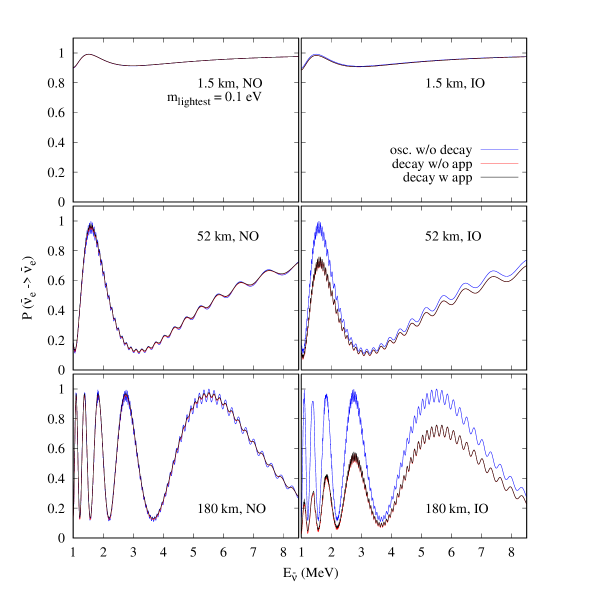
Figure 1: The effective electron anti-neutrino disappearance probability as a function of anti-neutrino energy for the Daya Bay (top panel), JUNO (middle panel) and KamLAND (bottom panel) experiments. The left (right) panel is for the NO (IO). We show the effective probabilities (defined as the ratio of the $\overline{\nu}_{e}$ flux arriving at the detector divided by the original flux at the detector in the absence of oscillation for a given neutrino energy) assuming standard oscillations without any decay (labeled “osc. w/o decay” in blue), with visible decay effect but without the daughter neutrino contribution (labeled “decay w/o app” in red) and with visible decay including the daughter neutrino contribution (labeled “decay w app” in black). For the visible decay, we consider $g_{\rm S}=g_{\rm PS}=0.2$ for NO and $g_{\rm S}=g_{\rm PS}=0.1$ for IO. Note that in some of the plots, the individual curves are too close together to be distinguished.

We first observe that the effect of decay is very noticeable in the case of IO (right panels) despite that the assumed magnitude of couplings for the IO case is smaller than that for NO , as can be seen in the right panels of Figure 1. It is because decay of the higher mass eigenstates $\overline{\nu}_{1}$ and $\overline{\nu}_{2}$, which occurs copiously in the reactor-produced $\overline{\nu}_{e}$ flux, leads to a much stronger reduction of the survival probability $P(\overline{\nu}_{e}\rightarrow\overline{\nu}_{e})$ than the NO case (see below). The effect can be seen clearly in the right panels of Figure 1 with the Majoron coupling constants $g_{\rm S}=g_{\rm PS}=0.1$. In the case of NO (left panels), on the other hand, the effect of decay is small, irrespective of whether the contribution from the daughter neutrinos is included or not. Unlike the case of IO, the reduction of the $\overline{\nu}_{e}$ flux is minor as the parent $\overline{\nu}_{3}$ component is small in reactor $\overline{\nu}_{e}$ due to suppression by small $|U_{e3}|^{2}=\sin^{2}\theta_{13}$. Therefore, the effect of visible decay in the case of NO is just to dampen the atmospheric-$\Delta m^{2}_{31}$ driven neutrino oscillation Abrahao:2015rba .

In visible decay, an additional effect, a pile-up of events at low energies due to the daughter neutrino contribution, should be observed. For the IO, for our choice of couplings $g_{\rm{S}}=g_{\rm{PS}}=0.1$ this effect is barely noticeable by eyes in Figure 1 but only for longer baseline as in the case of KamLAND at lower energies as a small difference between the cases without (red curves) and with (black curves) daughter contributions. We confirmed that by using somewhat larger values of couplings the pile-up effect become more prominent but its effect is tiny in any case because of small ($\propto|U_{e3}|^{2}$) $\overline{\nu}_{e}$ component in the decay product $\overline{\nu}_{3}$. The effect is negligible for the NO because the decay effect itself is small. However, we include the daughter neutrino contribution for both NO as well as IO, irrespective of its importance – on which some comments will follow later.

4 The oscillation probabilities with neutrino decay

We first recapitulate the formulas of the neutrino oscillation probabilities in the simultaneous presence of flavor oscillations and decay Kim:1990km ; Lindner:2001fx ; PalomaresRuiz:2005vf ; Coloma:2017zpg . We treat the system as in vacuum which is a good approximation for the reactor neutrino experiments.

4.1 Neutrino decay: General formula

We start by examining a generic case in which each of the three massive neutrinos oscillate and decay at the same time. When a neutrino of flavour $\alpha$ with energy $E_{\alpha}$ is produced at the distance $L=0$, the differential probability that a neutrino of flavour $\beta$ with energy in the interval $E_{\beta}+dE_{\beta}$ is detected at the distance $L$, can be written as Lindner:2001fx ; PalomaresRuiz:2005vf ; Coloma:2017zpg

$$\frac{dP_{\nu_{\alpha}^{r}\rightarrow\nu_{\beta}^{s}}}{dE_{\beta}}\left(E_{\alpha},E_{\beta},L\right) = \left|\sum_{i}U_{\beta i}^{(s)}U_{\alpha i}^{(r)*}\exp\left[-i\frac{m_{i}^{2}L}{2E_{\alpha}}\right]\exp\left[-\frac{1}{2}\left(\frac{\tau_{i}}{m_{i}}\right)^{-1}\frac{L}{E_{\alpha}}\right]\right|^{2}\delta(E_{\alpha}-E_{\beta})~{}\delta_{rs}$$ (2)

$$+ \int^{L}_{0}dL^{\prime}\left|\mathcal{A}_{\nu_{\alpha}^{r}\rightarrow\nu_{\beta}^{s}}\left(E_{\alpha},E_{\beta},L^{\prime}\right)\right|^{2}.$$

In Eq. (2), $\tau_{i}$ and $m_{i}$ represent $\nu_{i}$’s proper lifetime and mass, respectively, and the indices $r$ and $s$ specify, respectively, parent and daughter neutrino helicities. The matrix element $U_{\beta i}^{(s)}=U_{\beta i}(U_{\beta i}^{\ast})$ corresponds to the case for positive (negative) helicity. The first term of the differential probability in Eq. (2) describes the contribution from a parent neutrino of flavor $\alpha$ which survived after propagating a distance $L$. The second term in Eq. (2) is the daughter contribution and contains the decay amplitude $\mathcal{A}_{\nu_{\alpha}^{r}\rightarrow\nu_{\beta}^{s}}\left(E_{\alpha},E_{\beta},L^{\prime}\right)$ defined by

$$\mathcal{A}_{\nu_{\alpha}^{r}\rightarrow\nu_{\beta}^{s}}\left(E_{\alpha},E_{\beta},L^{\prime}\right)=\underset{i\neq j}{\sum^{3}_{i=1}\sum^{3}_{j=1}}\left(U^{r}_{\alpha i}\right)^{\ast}\left(U^{s}_{\beta j}\right)e^{-iE^{s}_{j}\left(L-L^{\prime}\right)}e^{-\frac{\alpha^{s}_{j}(L-L^{\prime})}{2E^{s}_{j}}}\sqrt{\frac{\alpha^{rs}_{ij}}{E^{r}_{i}}}\sqrt{\eta_{ij}}e^{-iE^{r}_{i}L^{\prime}}e^{-\frac{\alpha^{r}_{i}L^{\prime}}{2E^{r}_{i}}}.$$ (3)

It describes contribution of daughter neutrino of energy $E_{\beta}$ produced by decay of a parent neutrino with energy $E_{\alpha}$ at a distance $L^{\prime}(<L)$. Here, $\alpha/E$ represents the partial or full decay rates and $\eta$ represents normalized energy distribution of the daughter neutrinos. To understand Eq. 3 in detail, please refer to Ref. Lindner:2001fx . The first term of Eq. (2) is often called the “invisible” contribution. But, the case that we examine in this paper has no invisible decay; the decay products always include active neutrinos and hence are always visible in principle. To prevent confusion we call the first and the second terms of Eq. (2) as the “parent” and “daughter” contributions, respectively. We remark that if a neutrino undergoes invisible decay, the differential probability is given by the first term of Eq. (2). Then, what is the difference between the invisible decay and the parent contribution of our visible decay? The answer is that in the case of un-observable final states (such as sterile neutrinos), the decay width $\Gamma=1/\tau$ does not contain information about the final states. Whereas in our case $\Gamma$, which is computed with the Majoron model, does contain information of final states, such as the mass of the daughter neutrino. The lightest neutrino mass dependence of the event spectrum will be demonstrated in Section 7.

4.2 Parent contribution in visible neutrino decay

Let us calculate the contribution from the parent neutrinos i.e, the first term in Eq. (2). It gives the whole contribution in the case of invisible neutrino decay. By the nature of this term, helicity flip cannot be involved in it. Then, after integration over the neutrino energy $E_{\alpha}$ we obtain ($i,j=1,2,3$)

$$P_{\alpha\beta}^{\text{parent}} = \left|\sum_{i}U_{\beta i}U_{\alpha i}^{*}\exp\left[-i\frac{m_{i}^{2}L}{2E_{\alpha}}\right]\exp\left[-\frac{1}{2}\left(\frac{\tau_{i}}{m_{i}}\right)^{-1}\frac{L}{E_{\alpha}}\right]\right|^{2}$$ (4)

$$= \sum_{i}|U_{\alpha i}|^{2}|U_{\beta i}|^{2}\exp\left(-\frac{m_{i}}{\tau_{i}}\frac{L}{E_{\alpha}}\right)$$

$$+2\sum_{j>i}U_{\beta i}U_{\alpha i}^{*}U_{\beta j}^{*}U_{\alpha j}\exp\left\{-\left(\frac{m_{j}}{\tau_{j}}+\frac{m_{i}}{\tau_{i}}\right)\frac{L}{2E_{\alpha}}\right\}\cos\left(\frac{\Delta m^{2}_{ji}L}{2E_{\alpha}}\right).$$

Using the standard parameterization of the flavor mixing matrix Tanabashi:2018oca , and substituting $\tau_{1},\tau_{2}\rightarrow\infty$ for the NO, we obtain for $\overline{\nu}_{e}\rightarrow\overline{\nu}_{e}$ channel

$$P_{\overline{e}\overline{e}}^{\text{parent}}\text{ (NO) }= \cos^{4}\theta_{12}\cos^{4}\theta_{13}+\sin^{4}\theta_{12}\cos^{4}\theta_{13}+\sin^{4}\theta_{13}\exp\left(-\frac{m_{3}}{\tau_{3}}\frac{L}{E_{\alpha}}\right)$$ (5)

$$+ \dfrac{1}{2}\sin^{2}2\theta_{12}\cos^{4}\theta_{13}\cos\left(\frac{\Delta m^{2}_{21}L}{2E_{\alpha}}\right)$$

$$+ \dfrac{1}{2}\sin^{2}2\theta_{13}\cos^{2}\theta_{12}\exp\left\{-\left(\dfrac{m_{3}}{\tau_{3}}\right)\frac{L}{2E_{\alpha}}\right\}\cos\left(\frac{\Delta m^{2}_{31}L}{2E_{\alpha}}\right)$$

$$+ \dfrac{1}{2}\sin^{2}2\theta_{13}\sin^{2}\theta_{12}\exp\left\{-\left(\frac{m_{3}}{\tau_{3}}\right)\frac{L}{2E_{\alpha}}\right\}\cos\left(\dfrac{\Delta m^{2}_{32}L}{2E_{\alpha}}\right).$$

And for the inverted mass ordering, on substituting $\tau_{3}\rightarrow\infty$, we get

$$P_{\overline{e}\overline{e}}^{\rm{parent}}\text{ (IO)}= \sin^{4}\theta_{13}$$ (6)

$$+ \cos^{4}\theta_{13}\left[\cos^{4}\theta_{12}\exp\left(-\frac{m_{1}}{\tau_{1}}\frac{L}{E_{\alpha}}\right)+\sin^{4}\theta_{12}\exp\left(-\frac{m_{2}}{\tau_{2}}\frac{L}{E_{\alpha}}\right)\right]$$

$$+ \frac{1}{2}\sin^{2}2\theta_{12}\cos^{4}\theta_{13}\exp\left\{-\left(\frac{m_{1}}{\tau_{1}}+\frac{m_{2}}{\tau_{2}}\right)\frac{L}{2E_{\alpha}}\right\}\cos\left(\frac{\Delta m^{2}_{21}L}{2E_{\alpha}}\right)$$

$$+ \frac{1}{2}\sin^{2}2\theta_{13}\cos^{2}\theta_{12}\exp\left\{-\left(\frac{m_{1}}{\tau_{1}}\right)\frac{L}{2E_{\alpha}}\right\}\cos\left(\frac{\Delta m^{2}_{31}L}{2E_{\alpha}}\right)$$

$$+ \frac{1}{2}\sin^{2}2\theta_{13}\sin^{2}\theta_{12}\exp\left\{-\left(\frac{m_{2}}{\tau_{2}}\right)\frac{L}{2E_{\alpha}}\right\}\cos\left(\frac{\Delta m^{2}_{32}L}{2E_{\alpha}}\right).$$

4.3 Daughter contribution in visible neutrino decay

We calculate the contribution of daughter neutrinos, the second term in Eq. (2). We assume that the couplings between the neutrinos and the Majoron are real quantities and hence there are no decay-related complex phases. Since we are interested only in the electron antineutrino disappearance probabilities here we drop the helicity indices $r$ and $s$ keeping in mind that the quantities correspond to antineutrinos and that only helicity preserving decays can be observed in reactor experiments. However, it should be noted that the full decay-widths include the sum over helicity-preserving as well as helicity-flipping partial decay-widths. In this work, we assume the CP-violating phase $\delta_{CP}$ as well as the Majorana phases to be 0. Thus, we can also ignore the complex conjugation of the flavor matrix elements.

The transition amplitude $\mathcal{A}_{\nu_{\alpha}\rightarrow\nu_{\beta}}\left(E_{\alpha},E_{\beta},L^{\prime}\right)$ for the NO where $\overline{\nu}_{3}$ decays to $\overline{\nu}_{1}$ or $\overline{\nu}_{2}$, is given by Lindner:2001fx ; PalomaresRuiz:2005vf ; Coloma:2017zpg

$$\mathcal{A}_{\nu_{\alpha}\rightarrow\nu_{\beta}}^{\rm NO}\left(E_{\alpha},E_{\beta},L^{\prime}\right)=\sum_{d=1,2}U_{\alpha 3}U_{\beta d}\sqrt{\Gamma_{3d}}\sqrt{W_{3d}}~{}e^{-iE_{\beta}\left(L-L^{\prime}\right)}e^{-iE_{\alpha}L^{\prime}}e^{-\Gamma_{3}L^{\prime}/2}.$$ (7)

Whereas the transition amplitude for the IO, where $\overline{\nu}_{2}$ or $\overline{\nu}_{1}$ decay to $\overline{\nu}_{3}$, takes the form

$$\mathcal{A}_{\nu_{\alpha}\rightarrow\nu_{\beta}}^{\rm IO}\left(E_{\alpha},E_{\beta},L^{\prime}\right)=\sum_{p=1,2}U_{\alpha p}U_{\beta 3}\sqrt{\Gamma_{p3}}\sqrt{W_{p3}}~{}e^{-iE_{\beta}\left(L-L^{\prime}\right)}e^{-iE_{\alpha}L^{\prime}}e^{-\Gamma_{p}L^{\prime}/2}.$$ (8)

Here $E_{\alpha}$ $=p_{\alpha}+m_{p}^{2}/(2p_{\alpha})$ represents the energy of the parent neutrinos while $E_{\beta}$ $=p_{\beta}+m_{d}^{2}/(2p_{\beta})$ represents the energy of the daughter neutrinos. $p_{\alpha}$ ($p_{\beta}$) represent the amplitude of the three-momentum of the parent (daughter) neutrinos while $m_{p}$ ($m_{d}$) represent their constituent mass eigenvalues respectively. We assume that the different mass eigenstates possess the same momentum and they are relativistic; thus substituting $p$ for $E$. In the above equations, $\Gamma_{ij}$ is the partial decay width and $W_{ij}$ represents the normalized energy distribution function for the daughter neutrino for the decay $\overline{\nu}_{i}\rightarrow\overline{\nu}_{j}$. The explicit formulas are given in the Appendix A.

Eqs. (7) and (8) describe the process in which $\nu_{\alpha}$ is produced at $L=0$, propagates as the parent neutrino $\nu_{p}$ to $L^{\prime}$, then it decays into the daughter state $\nu_{d}$ at this distance $L^{\prime}$ and is detected as $\nu_{\beta}$ at $L$ > $L^{\prime}$ after traversing the distance $L-L^{\prime}$. In the NO, $p=3$ and $d=1,2$, while in the IO $p=1,2$ and $d=3$.

Using the Eq. (7) we can compute the visible decay term in Eq. (2), we find that for the NO,

$$\int^{L}_{0}\left|\mathcal{A}_{\nu_{\alpha}\rightarrow\nu_{\beta}}\right|^{2}dL^{\prime}=\left(U_{\alpha 3}\right)^{2}\sum^{2}_{j=1}\sum^{2}_{k=1}U_{\beta j}U_{\beta k}\sqrt{\Gamma_{3j}\Gamma_{3k}}\sqrt{W_{3j}W_{3k}}\left(\frac{e^{-\Gamma_{3}L}-e^{-i\frac{\Delta m^{2}_{jk}L}{2E_{\beta}}}}{i\frac{\Delta m^{2}_{jk}}{2E_{\beta}}-\Gamma_{3}}\right)$$ (9)

and for the IO,

$$\int^{L}_{0}\left|\mathcal{A}_{\nu_{\alpha}\rightarrow\nu_{\beta}}\right|^{2}dL^{\prime}=\left(U_{\beta 3}\right)^{2}\sum^{2}_{j=1}\sum^{2}_{k=1}U_{\alpha j}U_{\alpha k}\sqrt{\Gamma_{j3}\Gamma_{k3}}\sqrt{W_{j3}W_{k3}}\left(\frac{1-e^{-\left(i\frac{\Delta m^{2}_{jk}}{2E_{\alpha}}+\frac{\Gamma_{j}+\Gamma_{k}}{2}\right)L}}{i\frac{\Delta m^{2}_{jk}}{2E_{\alpha}}+\frac{\Gamma_{j}+\Gamma_{k}}{2}}\right)$$ (10)

In Eqs. (9) and (10) above, the imaginary terms change sign under an interchange of the indices $j$ and $k$; hence the sums are real.

5 Sketchy descriptions of KamLAND and JUNO

In this section, we briefly describe the details of KamLAND and JUNO, which are phenomenologically relevant to our work.

5.1 KamLAND

The KamLAND (Kamioka Liquid Scintillator Antineutrino Detector) reactor neutrino experiment consists of 1 kton of highly purified liquid scintillator detector based in Japan. KamLAND detects neutrinos coming from 16 nuclear power plants with a range of distances that go from $140$ km to $215$ km. The average distance corresponds to $\sim 180$ km. The experiment ran in the reactor anti-neutrino mode from 2002 to 2012, collecting a total exposure of $4.90\times 10^{32}$ target-proton-years. We consider the data presented in Gando:2013nba to perform our analysis of neutrino decay. The information regarding backgrounds and systematic uncertainties have also been taken from Gando:2013nba . The expected advantage of KamLAND over JUNO to study the decay effect is, as we could see in the plot of probabilities in Figure 1, the longer average baseline, which is about 3.4 times the JUNO’s baseline, leading to larger decay effects.

5.2 JUNO

The JUNO (Jiangmen Underground Neutrino Observatory) experiment An:2015jdp is a future neutrino experiment that will be based in China. It is expected to start taking data from the year 2022. JUNO has been designed with the primary goal to measure the neutrino mass ordering but it will also be able to measure the oscillation parameters such as $\theta_{12}$, $\Delta m^{2}_{21}$ and $\Delta m^{2}_{31}$ with much better precision. The detector consists of a 20 kton fiducial mass of liquid scintillator and is located at an average distance of $\sim 53$ km from Yangjiang and Taishan nuclear power plants. The remote reactor cores at Daya Bay and Huizhou will also have a small contribution to the total flux arriving at the JUNO detector. In our experimental set-up, we consider the various reactor cores with different thermal powers and baselines as described in Table 2 of An:2015jdp . The description of backgrounds and systematic uncertainties have been taken from An:2015jdp . The exposure is set such that a total of $140,000$ events are obtained (including the backgrounds).

The signal in both of the experiments is the inverse beta-decay (IBD) events in the energy range $\sim\left[1.8,8\right]$ MeV, which essentially determines the electron antineutrino disappearance probability for a given, relatively well known IBD reaction cross-sections. The main background in a search for visible neutrino decay in JUNO is the geo-neutrino events at low energies. We consider their contributions similarly as done in Abrahao:2015rba . The expected advantage of JUNO over KamLAND to study the neutrino decay is (i) much larger statistics and (ii) better energy resolution which is crucial for the case of NO as we will see later.

To simulate the KamLAND and the JUNO experiments, we have used the GLoBES Huber:2004ka ; Huber:2007ji software package. The event rates and statistical-$\chi^{2}$ calculations have also been performed using GLoBES.

6 Features of event rates in the presence of decay

In this section, using the observed and the expected event rates at KamLAND and JUNO, respectively, we stress upon the following two features that crucially affect the results in the presence of visible decay.

1. Dependence of event rates on the neutrino mass ordering, and

2. Dependence of event rates on the lightest neutrino mass.

Note that the lightest neutrino is $\nu_{3}$ in the case of IO, and $\nu_{1}$ in the case of NO.

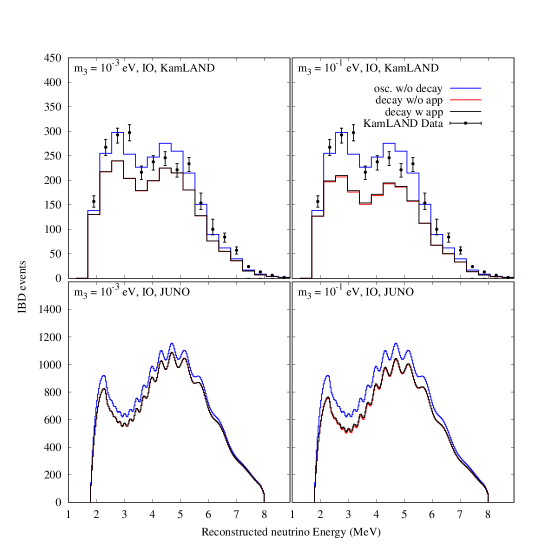
Figure 2: Events rates vs. reconstructed neutrino energy assuming IO for KamLAND (top panel) and JUNO (bottom panel) with and without the decay effects. The left (right) panels correspond to the choice of $m_{\rm lightest}=10^{-3}$ eV ($m_{\rm lightest}=10^{-1}$ eV). We show the rates for standard oscillations without any decay (labeled “osc. w/o decay” in blue), visible decay without the daughter neutrino contribution (labeled “decay w/o app” in red) and visible decay including the daughter contribution (labeled “decay w app” in black). For the visible decay, we consider $g_{\rm S}=g_{\rm PS}=0.1$. For these values of the couplings and $m_{\rm lightest}$, the values of $\tau_{2}/m_{2}$ are $6.6\times 10^{-10}\rm{s/eV}$ (for $m_{3}=10^{-3}\rm{eV}$) and $3.7\times 10^{-10}\rm{s/eV}$ (for $m_{3}=10^{-1}\rm{eV}$). Also shown are the observed KamLAND data indicated by the black solid circles with error bars which are taken from Gando:2013nba .

In Figs. 2 and  3, we show the event rates for the IO and NO respectively. The top panels in both of these figures show the observed event rates at the KamLAND experiment with 17 bins of 425 MeV each lying in the reconstructed energy range $\left[1.7,8.925\right]$ MeV. The bottom panels of these figures show the expected event rates for the JUNO experiment with a total of 200 bins (corresponding to the bin width of 0.031 MeV) in the reconstructed energy interval $\left[1.8,8.0\right]$ MeV. In Figs. 2 and  3, the event rates include the signal as well as the background geo-neutrinos. In the left and the right panels, we assume $m_{\rm{lightest}}=10^{-3}$ eV and $m_{\rm{lightest}}=10^{-1}$ eV, respectively. We assume the following values of the oscillation deSalas:2017kay and decay parameters to generate these event rates.

• Inverted Ordering: $\theta_{12}=34.5^{\circ}$, $\theta_{13}=8.53^{\circ}$, $\theta_{23}=47.9^{\circ}$, $\Delta m^{2}_{21}=7.55~{}\times~{}10^{-5}~{}\rm{eV}^{2}$, $|\Delta m^{2}_{31}|=2.42\times 10^{-3}~{}\rm{eV}^{2},~{}g_{\rm{S}}=g_{\rm{PS}}=0.1$ .

• Normal Ordering: $\theta_{12}=34.5^{\circ}$, $\theta_{13}=8.45^{\circ}$, $\theta_{23}=47.7^{\circ}$, $\Delta m^{2}_{21}=7.55~{}\times~{}10^{-5}~{}\rm{eV}^{2}$, $|\Delta m^{2}_{31}|=2.50\times 10^{-3}~{}\rm{eV}^{2},~{}g_{\rm{S}}=g_{\rm{PS}}=0.2$.

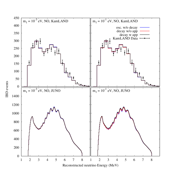
Figure 3: Events rates vs. reconstructed neutrino energy assuming NO for KamLAND (top panel) and JUNO (bottom panel) with and without the decay effects. The left (right) panels correspond to the choice of $m_{\rm lightest}=10^{-3}$ eV ($m_{\rm lightest}=10^{-1}$ eV). We show the rates for standard oscillations without any decay (labeled “osc. w/o decay” in blue), visible decay without the daughter neutrino contribution (labeled “decay w/o app” in red) and visible decay including the daughter contribution (labeled “decay w app” in black). For the visible decay, we consider $g_{\rm S}=g_{\rm PS}=0.2$. For these values of the couplings and $m_{\rm lightest}$, the values of $\tau_{3}/m_{3}$ are $8.3\times 10^{-11}\rm{s/eV}$ (for $m_{1}=10^{-3}\rm{eV}$) and $4.6\times 10^{-11}\rm{s/eV}$ (for $m_{1}=10^{-1}\rm{eV}$). Also shown are the observed KamLAND data indicated by the black solid circles with error bars which are taken from Gando:2013nba .

From Figure 2, as expected from the probabilities shown in the right panels of Figure 1, we see that the effects of decay are significant for IO. This is because, for IO, $\overline{\nu}_{2}$ or $\overline{\nu}_{1}$ mass eigenstate decays to $\overline{\nu}_{3}/\nu_{3}$. Thus, the decay is expected to affect the $\Delta m^{2}_{21}$-driven oscillations. For KamLAND and JUNO, these oscillations are much larger in magnitude compared to $\Delta m^{2}_{31}$-driven-oscillations due to the large value of $\theta_{12}$. Therefore, decay effects are also large. Furthermore, when one considers the full visible decay including the contribution from daughter neutrinos, a pile-up of events at lower energies is noticeable for $m_{\rm{lightest}}$ =$10^{-1}$ eV (see text below for the $m_{\rm{lightest}}$ dependence on the decay effect). However, this is still a small effect as the appearance of $\overline{\nu}_{e}$ is suppressed due to the smallness of $|U_{e3}|^{2}$. We note that the case considered to generate the results shown in Figure 2, $g_{\rm{S}}=g_{\rm{PS}}=0.1$ for the IO case, is turned out to be excluded as we will see later.

The decay effects in the event spectrum also depend on the lightest neutrino mass as can be seen by comparing the left and right panels in Figure 2. We first observe that, as long as the results shown in Figure 2 is concerned, for relatively small ($\raise 1.29167pt\hbox{$\;<$\kern-7.5pt\raise-4.73611pt\hbox{$\sim\;$}}0.1$) values of couplings, the lightest neutrino mass dependence comes mainly from the mass dependence in the visible part of the probabilities given in Eqs. (5) and (6). We remind the readers that the daughter contributions coming from Eqs. (9) or  (10) in the effective probabilities shown in Figure 1 is quite small, which should be reflected in the event number distributions.

However, expressions shown in Eqs. (5) and (6) are not useful to understand the lightest neutrino mass dependence we can see in Figure 2 since the lifetime $\tau_{i}$ appears in these equations also depend on neutrino masses. Therefore, we should take a closer look at the expressions of $\Gamma$ functions given in the Appendix, taking into account that $\Gamma_{ij}=m_{i}/(\tau_{i}E)$ for the decay mode of $\nu_{i}\to\nu_{j}$.

By looking into the expression of decay width $\Gamma$ functions in Eq. (17), we can say that the origin of the lightest neutrino mass dependence comes from two parts: (i) the part which is given by the square of the mass of parent neutrino, $m_{i}^{2}$, a factor common for both helicity flipping and conserving processes, and (ii) the part which is described by the dimensionless functions $f(x),h(x)$ and $k(x)$ shown in the Appendix, which have dependence on the both parent and daughter masses of neutrinos as well as on the helicity of daughter neutrino, if it is flipped or conserved.

Let us first take a look the part (ii) which looks more complicated. For the case $g_{\rm S}~{}=~{}g_{\rm PS}$, the total rate coming from this part is proportional to the sum of $(f(x)+h(x)+k(x))/x$ as we can see from Eq. (17) in Appendix A. We observe that the variation of the lightest neutrino mass have little impact on these functions (mainly due to $f(x)$ which is dominant), and therefore induces little impact on the total rate, at most a factor of $\sim$ 2-3 for both mass orderings (see Figure 1 in Ref. Coloma:2017zpg for the NO where $f(x)/x,h(x)/x,k(x)/x$ is shown as a function of $x$).

On the other hand, the part (i), mass square of the parent neutrinos, ${m_{i}^{2}}$, has stronger dependence on the lightest neutrino masses for the both mass orderings. In the IO, for the case of $\nu_{2}\to\nu_{3}$ decay, the parent mass is $m_{2}=\sqrt{m_{\rm lightest}^{2}+\Delta m_{21}^{2}+|\Delta m_{31}^{2}|}$ which implies that the two different values of lightest neutrino mass lead to $m^{2}_{2}\simeq\Delta m^{2}_{\rm atm}=2.40\times 10^{-3}$ eV² for $m_{\text{lightest}}=10^{-3}$ eV, and $m^{2}_{2}\simeq m_{\rm lightest}^{2}=10^{-2}$ eV² for $m_{\text{lightest}}=10^{-1}$ eV. As a result, the decay width is an order of magnitude larger in the case of $m_{\text{lightest}}=10^{-1}$ eV, leading to the small but visible difference between the left and right panels for the IO in Figure 2. In the NO, the situation is similar but $m_{\text{lightest}}$ dependence is not visible in Figure 3 because the impact of decay itself is small due to small value of $\theta_{13}$ as explained in the end of Section 3. We must remind the readers that these particular dependences of the decay rate on the parent neutrino mass may be model-dependent, which should be kept in mind in interpreting our results.

From Figure 3, for the case of NO, it can be seen that the KamLAND experiment is almost insensitive to the decay of $\overline{\nu}_{3}$ to $\overline{\nu}_{2}/\nu_{2}$ or $\overline{\nu}_{1}/\nu_{1}$. This is expected because the $\Delta m^{2}_{31}$-driven oscillations are averaged out at the baselines relevant to the KamLAND experiment, and therefore, the distortions in the spectrum due to decay cannot be seen. Though a small pile-up of events due to daughter neutrinos is seen, KamLAND cannot place a useful bound on $\tau_{3}$ due to the appearance of daughter neutrinos in the NO case, because they are too small to be statistically significant. For the case of the JUNO experiment, we find that for the NO there is a very small effect of decay on the event rates. In the NO, small $s^{2}_{13}$ suppresses decay of $\overline{\nu}_{3}$ into $\overline{\nu}_{2}/\nu_{2}$ or $\overline{\nu}_{1}/\nu_{1}$, whose effect is mainly just to dampen the $\Delta m^{2}_{31}$-driven oscillations, as explored previously in Ref. Abrahao:2015rba .

In the case of IO, because of more than a factor of three longer average baselines of KamLAND which leads to the larger effect of neutrino decay than that for JUNO, KamLAND should be able to place a stronger constraint on $\nu_{2}$ lifetime, if the number of events was similar to that of JUNO. However, this advantage is largely compensated by much lower statistics of KamLAND with the total number of events, 2611 (including backgrounds) Gando:2013nba , which is smaller than those assumed for JUNO by a factor of 54. Therefore, interpretation of the KamLAND bound on $\nu_{2}$ lifetime, which is only slightly better than JUNO as will be reported in Section 7, must be done with care.

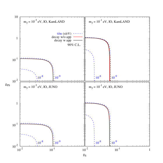
Figure 4: Decay constraints and sensitivity plots for KamLAND (top panel) and JUNO (bottom panel). We show the $90\%$ C.L. contours in the $g_{\rm{S}}-g_{\rm{PS}}$ plane. The true mass ordering is assumed to be inverted. The left (right) panel is for $m_{\rm lightest}=10^{-3}$ eV ($10^{-1}$ eV). The red curve (labeled “decay w/o app”) corresponds to visible decay including the contribution from the parent neutrinos only while the black curve (labeled “decay w app”) corresponds to visible decay including the contributions from both parents as well as the daughter neutrinos. The blue curves show the respective values of $g_{\rm{S}},g_{\rm{PS}}$ which give $\left(\tau/m\right)_{\rm{heaviest}}=10^{-8},10^{-9}$ s/eV.

7 Constraints on visible neutrino decay by KamLAND and JUNO

In this section, we present the results of our analysis to obtain the constraints on visible neutrino decay imposed by the KamLAND data, and by a simulated data of JUNO assuming the total number of events equals to 140,000 which can be obtained by the exposure of $\sim$ 220 GW$\cdot$years (total reactor thermal power times running period with $\sim$ 90% of reactor avilability assuming 100% detection efficiency). We exhibit the obtained constraints by drawing the $90\%$ C.L. exclusion contours in the $g_{\rm S}-g_{\rm PS}$ plane in Figure 4 for IO, and in Figure 5 for NO, for both KamLAND and JUNO. To translate these results to the constraints on the ratio of lifetime $\tau$ to the mass $m$, we show the equal $\tau/m$ contours as a function of $g_{\rm S}$ and $g_{\rm PS}$ in Figs. 4 and 5.

7.1 Analysis procedure

We now describe the numerical procedure for calculating the $\chi^{2}$ for excluding decay. For KamLAND, we consider the data presented in Gando:2013nba while for JUNO, we simulate the “true events rates” assuming that neutrinos undergo only standard oscillations and that no neutrino decay occurs. To simulate the true events rates in the case of JUNO, we take the values of the oscillation parameters used in Section 6.

We then “fit” the observed/simulated data with the calculated event rates assuming the existence of neutrino decay, by varying freely the values of $g_{\rm S}$ and $g_{\rm PS}$ in addition to varying the standard oscillation parameters $\theta_{12}$, $\theta_{13}$, $\Delta m^{2}_{21}$ and $|\Delta m^{2}_{31}|$ in their currently-allowed $3\sigma$ ranges. Note that in the fit we keep the test mass ordering same as the true one. These events rates are called the “test event rates”. The binned-$\chi^{2}$ are calculated using GLoBES including the marginalization over the systematic uncertainties. We also add $\chi^{2}$ due to the Gaussian priors corresponding to the test oscillation parameters that are varied in the fit. The formula for the total $\chi^{2}$ is given by

$$\chi^{2}_{\rm{total}} = \sum_{i=1}^{n}2\left[F_{i}\left(1+\xi_{1}+\xi_{2}\right)-D_{i}+D_{i}\ln\left(D_{i}/F_{i}\left(1+\xi_{1}+\xi_{2}\right)\right)\right]$$ (11)

$$+ \sum_{k}\left(\xi_{k}/\sigma_{k}\right)^{2}+\sum_{j}(\theta_{j}-\theta_{j}^{\rm{bf}})^{2}/\sigma_{j}^{2}.$$

Here, $n=17$ ($n=200$) is the total number of energy bins for KamLAND (JUNO). $F_{i}$ and $D_{i}$ are the theoretical number of events and the observed number of events, respectively, in a given $i$-th bin. $\xi_{k}$ are the systematic uncertainty parameters with standard deviation $\sigma_{k}$; and $\theta_{j}^{\rm{bf}}$ is the best fit value of a given oscillation parameter $\theta_{j}$ (that are varied in the fit) with a $1\sigma$ uncertainty $\sigma_{j}$. For both KamLAND and JUNO, we consider an overall normalization error of $\xi_{1}=5\%$ for signal and $20\%$ for the background events and an energy calibration error of $\xi_{2}=3\%$. For a given choice of the test decay parameters $g_{\rm S}$ and $g_{\rm PS}$, we select the least $\chi^{2}_{\rm{total}}$ that is obtained after marginalizing over all the test oscillation parameters. The $\Delta\chi^{2}$ for a given $g_{\rm S}$ and $g_{\rm PS}$ is obtained through: $\Delta\chi^{2}=\chi^{2}_{\rm total}-\chi^{2}_{\rm total,~{}smallest}$. We show the resulting contours corresponding to $\Delta\chi^{2}$ =4.61 for 2 degree of freedom (DOF) as a function of the test $g_{\rm S}$ and $g_{\rm PS}$.

7.2 KamLAND and JUNO bounds on neutrino decay: the inverted mass ordering

We first discuss the potential of the experiments to exclude visible decay for the case of IO, shown in Figure 4. The top panels show the results for KamLAND while the bottom panels show the results for JUNO. The left panels in these figures are for $m_{\rm{lightest}}=10^{-3}$ eV while the right panels are for $m_{\rm{lightest}}=10^{-1}$ eV.

From the top panels of Figure 4, we find that KamLAND excludes $g_{\rm S}~{}\gtrsim 0.11$ and $g_{\rm PS}\gtrsim 0.11$ for $m_{\rm{lightest}}=10^{-3}$ eV at 90% C.L. For $m_{\rm{lightest}}=10^{-1}$ eV, $g_{\rm S}\gtrsim 0.06$ and $g_{\rm PS}\gtrsim 1.00$ are excluded. In either case, the constraints correspond to the exclusion of $\tau/m~{}\lesssim 1.1\times 10^{-9}~{}\rm{s/eV}$. From the lower panel, we see that for $m_{\rm{lightest}}=10^{-3}$ eV, JUNO can exclude neutrino visible decay at $90\%$ C.L. for IO if $g_{\rm S}\gtrsim 0.11$ and $g_{\rm PS}\gtrsim 0.11$. For $m_{\rm{lightest}}=10^{-1}$ eV, if $g_{\rm S}\gtrsim 0.05$ and $g_{\rm PS}~{}\gtrsim 1.00$, JUNO can exclude neutrino decay at $90~{}\%$ C.L.. For both KamLAND and JUNO, the constraint for the pseudo-scalar coupling for $m_{\rm{lightest}}=10^{-1}$ eV is much weaker because the functions $h(x)$ and $k(x)$ in $\Gamma$ are much smaller than $f(x)$ for $m_{\rm{lightest}}=10^{-1}$ eV, see Figure 1 in Coloma:2017zpg . Expressed in terms of $\tau/m$, for IO, JUNO excludes $\tau/m\lesssim 1.1\times 10^{-9}~{}\rm{s/eV}$, which happened to be the same value as that of KamLAND. We see that inclusion of the daughter neutrino contributions does not affect in any significant way the decay exclusion sensitivity. In all the panels, the two curves with and without the daughter’s contributions are nearly coincident.

It is remarkable that despite that the number of events obtained by KamLAND used for our analysis is 54 times smaller than that for JUNO (2611 vs 140,000), both experiments give very similar bounds (sensitivities). As mentioned at the end of the previous section, we understand that this is mainly because of more than 3 times larger average baseline of KamLAND ($\sim$ 180 km) compared to JUNO ($\sim$ 53 km) which can largely compensate the much smaller statistics of KamLAND.

Let us now try to understand qualitatively the dependence of the value of $m_{\text{lightest}}$ on the sensitivities to $g_{\rm S}$ and $g_{\rm PS}$ we can see in Figure 4. Since the contributions from daughter neutrinos are small, we just need to pay attention to the decay width $\Gamma$ in Eq. (17), in particular for the helicity conserving case $r=s$ which is dominant.

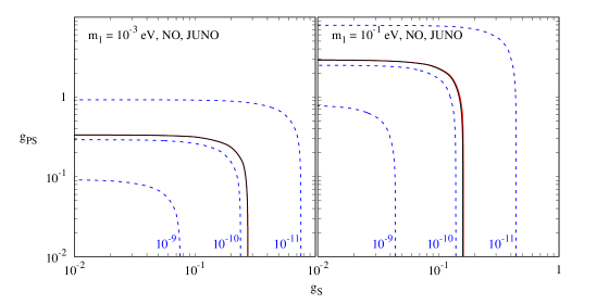
Figure 5: Decay sensitivity plots for JUNO. We show the $90\%$ C.L. contours in the $g_{\rm{S}}-g_{\rm{PS}}$ plane for $m_{\rm lightest}=10^{-3}$ eV ($10^{-1}$ eV) in the left (right) panel. The true mass ordering is assumed to be normal. The same notation apply as in Figure 4. The blue curves show the respective values of $g_{\rm{S}},g_{\rm{PS}}$ which give $\left(\tau/m\right)_{\rm{heaviest}}=10^{-9},10^{-10},10^{-11}$ s/eV.

We first note that in the limit of vanishing $m_{\text{lightest}}$, which corresponds to $x\to\infty$, the functions $f(x)$, $h(x)$ and $k(x)$ given in eq.(18) tend to become equal. See also Figure 1 of Ref. Coloma:2017zpg . It implies that both couplings, $g_{\rm S}$ and $g_{\rm PS}$, contribute equally to neutrino decay, which explains why the bounds are nearly symmetric to $g_{\rm S}$ and $g_{\rm PS}$ in the case of $m_{\text{lightest}}=10^{-3}$ eV.

On the other hand, as the assumed true value of $m_{\text{lightest}}$ is increased (or $x$ is decreased), the function $f(x)/x$ ($h(x)/x$) is increased (decreased), as can be seen from the first equation in (17) and also from Figure 1 of Ref. Coloma:2017zpg . It means that the scalar (pseudo-scalar) coupling $g_{\rm S}$ ($g_{\rm PS}$) becomes more (less) important for decay. This is the reason why the bound on the scalar (pseudo-scalar) coupling become tighter (milder) at a large value of $m_{\text{lightest}}~{}=~{}10^{-1}$ eV independent of the mass orderings.

7.3 JUNO bound on neutrino decay: the normal mass ordering

We consider only the JUNO experiment as it was shown previously (see Section 6) that there is little sensitivity to the decay $\nu_{3}\rightarrow\nu_{1,2}$ in KamLAND. JUNO will be able to place a limit on the decay effect because of the much larger statistics and good energy resolution which allows to detect the damping-like effect in the $\Delta m^{2}_{31}$ driven oscillation we can see in the left middle panel of Figure 1. From Figure 5, we see that for $m_{\rm{lightest}}=10^{-3}$ eV, JUNO can exclude neutrino visible decay at $90\%$ C.L. if $g_{\rm S}\gtrsim 0.28$ and $g_{\rm PS}\gtrsim 0.33$. For $m_{\rm{lightest}}=10^{-1}$ eV, JUNO can exclude neutrino decay at $90\%$ C.L. if the mass ordering is normal and $g_{\rm S}\gtrsim 0.16$ and $g_{\rm PS}\gtrsim 2.90$. The constraint on $g_{\rm PS}$ is much weaker mainly due to the same reason described in Section 7.3 for the IO case. Expressed in terms of $\tau/m$, we find that for NO, JUNO excludes $\tau/m\lesssim 7.5\times 10^{-11}~{}\rm{s/eV}$. A comparison between Figs. 4 and 5 indicates that the bounds crucially depend on the choice of the mass ordering: the constraints are milder in the NO by an order of magnitude. In the NO, as in the case of IO, the daughter neutrinos give essentially no contribution to exclusion of decay, leading to almost complete degeneracy of the red and the black curves in Figure 5.

Experiment	(ordering, $m_{\rm{lightest}}$)	$g_{\rm{S}}$	$g_{\rm{PS}}$	$\tau/m$ (s/eV)
KamLAND	(IO, $10^{-3}$ eV)	$0.11$	$0.11$	$1.1\times 10^{-9}$
KamLAND	(IO, $10^{-1}$ eV)	$0.06$	$1.00$	$1.1\times 10^{-9}$
JUNO	(IO, $10^{-3}$ eV)	$0.11$	$0.11$	$1.1\times 10^{-9}$
JUNO	(IO, $10^{-1}$ eV)	$0.05$	$1.00$	$1.1\times 10^{-9}$
JUNO	(NO, $10^{-3}$ eV)	$0.28$	$0.33$	$7.5\times 10^{-11}$
JUNO	(NO, $10^{-1}$ eV)	$0.16$	$2.90$	$7.5\times 10^{-11}$

Table 2: The $90\%$ C.L. upper bound on the couplings and the lower bound on the lifetime of active neutrinos for the given mass ordering and the values of the lightest neutrino mass, obtained through the sensitivity analyses of the experiments KamLAND and JUNO. The values of $g_{\rm{S}}$ and $g_{\rm{PS}}$ shown correspond to $\Delta\chi^{2}=4.61$ for 2 DOF. The value of $\tau/m$ shown is calculated for the given $m_{\rm{lightest}}$ and the obtained value of $g_{\rm{S}}$ again for 2 DOF.

In Table 2, we summarize the constraints obtained by KamLAND and JUNO discussed in this section.

8 Conclusions

In this work, we have discussed the effect of visible neutrino decay which can be detected by observing the positron energy spectrum due to the IBD reaction in reactor neutrino experiments. Modifications of the spectrum not only in the shape but also in the normalization are important. We have obtained the constraints on the lifetime of higher-mass state neutrinos ($\nu_{3}$ in the NO, and $\nu_{2}$ or $\nu_{1}$ in the IO) in medium and long-baseline reactor experiments.

We have used the Majoron model to calculate the neutrino decay rate. We took the two experimental settings, KamLAND and JUNO. They are the most relevant ones because of the long baseline, $\sim 180$ km for KamLAND, and high energy resolution $\raise 1.29167pt\hbox{$\;<$\kern-7.5pt\raise-4.73611pt\hbox{$\sim\;$}}3\%$ expected for JUNO in construction. For KamLAND we use the latest data, and for JUNO we assume the exposure of about 220 GW$\cdot$years which would produce $1.4\times 10^{5}$ events. In comparison with the constraints on neutrino decay often expressed as the bound on $\tau/m$ ($\tau_{3}/m_{3}$ for the NO, and $\tau_{2}/m_{2}$ for the IO) at 90% C.L. for 1 degree of freedom, we have provided the corresponding information in Table 3.

Experiment	(ordering, $m_{\rm{lightest}}$)	$\tau/m$ (s/eV)
KamLAND	(IO, $10^{-3}$ eV)	$1.4\times 10^{-9}$
KamLAND	(IO, $10^{-1}$ eV)	$1.4\times 10^{-9}$
JUNO	(IO, $10^{-3}$ eV)	$1.4\times 10^{-9}$
JUNO	(IO, $10^{-1}$ eV)	$1.4\times 10^{-9}$
JUNO	(NO, $10^{-3}$ eV)	$1.0\times 10^{-10}$
JUNO	(NO, $10^{-1}$ eV)	$1.0\times 10^{-10}$

Table 3: The $90\%$ C.L. lower bound on the lifetime / mass of active neutrinos for the given mass ordering and the values of the lightest neutrino mass, obtained through the sensitivity analyses of the experiments KamLAND and JUNO. The values of $\tau/m$ = $\tau_{3}/m_{3}$ ($\tau_{2}/m_{2}$) for the normal (inverted) ordering, calculated for a given $m_{\rm{lightest}}$, shown correspond to $\Delta\chi^{2}=2.71$ for 1 DOF.

We found that the lifetime bounds depend crucially on whether the neutrino mass ordering is normal or inverted. Roughly speaking, the results we obtained for JUNO shows that for the IO, the bounds are better than the one for the NO approximately by a factor of 20. In looking into closer detail, KamLAND is insensitive to the decay of $\nu_{3}$ in the case of NO because of insufficient energy resolution to measure small wiggles of the atmospheric-scale high-frequency oscillations and statistically-insignificant pile-up of events due to daughter neutrinos at lower energies. JUNO, on the other hand, can rule out $\tau/m\lesssim 1.0\times 10^{-10}$ s/eV for the $\nu_{3}$ mass eigenstate. We note that this value is quite similar and consistent with the bound of 9.3 $\times 10^{-11}$ s/eV for the same confidence level (90% C.L.), obtained in Abrahao:2015rba where the invisible neutrino decay for JUNO was studied. For the case of IO, the bounds of roughly the same order of magnitude are obtained on the decay of the $\nu_{2}$ mass eigenstate by both KamLAND and JUNO. We find that $\tau/m\lesssim 1.4\times 10^{-9}$ s/eV is ruled out by both KamLAND and JUNO for the $\nu_{2}$ mass eigenstate.

We have observed that, in each of these cases, there is no significant improvement in the sensitivity by including the daughter neutrino contributions in the analyses. It is because the effect is suppressed through $|U_{e3}|^{2}$, which is small. However, in the case of IO, a decrease of $\overline{\nu}_{e}$ flux by the decay of $\overline{\nu}_{2}$ and $\overline{\nu}_{1}$ mass eigenstates produces a clear signature of neutrino decay, yielding a stringent lifetime bound mentioned above. For the NO, neutrino decay acts merely as a damping effect of the fast $\Delta m^{2}_{31}$-driven oscillations both in JUNO and KamLAND, rendering detection of decay effect harder, in particular, for the latter. We also mention that our lifetime bound depends on $m_{\rm{lightest}}$ through $m_{\rm{lightest}}$ dependence of the decay rate.

Appendix A Auxiliary formulae

We have the auxiliary functions, respectively the decay rate, $\Gamma^{rs}_{ij}$ of $\nu^{(r)}_{i}\to\nu^{(r)}_{j}$ of initial mass state of mass $m_{i}$ and helicity r and final neutrino mass $m_{j}$ and helicity s , and normalized spectrum of daughter distribution, $W^{rs}_{ij}(E_{\alpha},E_{\beta})$ with $E_{\alpha}$ the energy of initial state and $E_{\beta}$ the energy of the final neutrino Lindner:2001fx ; PalomaresRuiz:2005vf ; Coloma:2017zpg

$$\Gamma^{rs}_{ij}=\left\{\begin{array}[]{l l}\frac{m_{i}^{2}}{16\pi E_{i}}\bigg{[}(g_{\rm S}^{ij})^{2}\left(\frac{f(x_{ij})}{x_{ij}}\right)+(g_{\rm PS}^{ij})^{2}\left(\frac{h(x_{ij})}{x_{ij}}\right)\bigg{]}\quad\phantom{lala}&r=s,\\[14.22636pt] \frac{m_{i}^{2}}{16\pi E_{i}}\left[((g_{\rm S}^{ij})^{2}+(g_{\rm PS}^{ij})^{2})\left(\frac{k(x_{ij})}{x_{ij}}\right)\right]&r\neq s\\ \end{array}\right.$$ (14)

$$W^{rs}_{ij}(E_{\alpha},E_{\beta})\equiv\dfrac{1}{\Gamma^{rs}_{ij}}\dfrac{d\Gamma^{rs}_{ij}(E_{\alpha},E_{\beta})}{dE_{\beta}}=\left\{\begin{array}[]{l l}\left(\dfrac{1}{E_{\alpha}}\right)\dfrac{(g_{\rm S}^{ij})^{2}(R+2)+(g_{\rm PS}^{ij})^{2}(R-2)}{(g_{\rm S}^{ij})^{2}f(x_{ij})+(g_{\rm PS}^{ij})^{2}h(x_{ij})}\quad\phantom{lala}&r=s,\\[14.22636pt] \left(\dfrac{1}{E_{\alpha}}\right)\dfrac{\frac{1}{x_{ij}}+x_{ij}-R}{k(x_{ij})}&r\neq s\end{array}\right.$$ (17)

where

$$R\equiv\dfrac{1}{x_{ij}}\dfrac{E_{\alpha}}{E_{\beta}}+x_{ij}\frac{E_{\beta}}{E_{\alpha}}$$

with $x_{ij}\equiv m_{i}/m_{j}>1$, and the functions $f(x),h(x),k(x)$ are defined in Eq. (18).

$$f(x) = \dfrac{x}{2}+2+\dfrac{2\ln(x)}{x}-\dfrac{2}{x^{2}}-\dfrac{1}{(2x^{3})}\,,$$

$$h(x) = \dfrac{x}{2}-2+\dfrac{2\ln(x)}{x}+\dfrac{2}{x^{2}}-\dfrac{1}{(2x^{3})}\,,$$ (18)

$$k(x) = \dfrac{x}{2}-\dfrac{2\ln(x)}{x}-\dfrac{1}{(2x^{3})}\,.$$

References

- (1) S. T. Petcov, The Processes in the Weinberg-Salam Model with Neutrino Mixing, Sov. J. Nucl. Phys. 25 (1977) 340.
- (2) W. J. Marciano and A. I. Sanda, Exotic Decays of the Muon and Heavy Leptons in Gauge Theories, Phys. Lett. 67B (1977) 303–305.
- (3) B. W. Lee and R. E. Shrock, Natural suppression of symmetry violation in gauge theories: Muon- and electron-lepton-number nonconservation, Phys. Rev. D 16 (Sep, 1977) 1444–1473.
- (4) R. E. Shrock, Electromagnetic Properties and Decays of Dirac and Majorana Neutrinos in a General Class of Gauge Theories, Nucl. Phys. B206 (1982) 359–379.
- (5) J. A. Frieman, H. E. Haber and K. Freese, Neutrino Mixing, Decays and Supernova Sn1987a, Phys. Lett. B200 (1988) 115.
- (6) Kamiokande-II collaboration, K. S. Hirata et al., Observation of a Neutrino Burst from the Supernova SN 1987a, Phys. Rev. Lett. 58 (1987) 1490–1493.
- (7) IMB Collaboration collaboration, R. M. Bionta et al., Observation of a Neutrino Burst in Coincidence with Supernova SN 1987a in the Large Magellanic Cloud, Phys. Rev. Lett. 58 (1987) 1494.
- (8) Z. G. Berezhiani and A. Y. Smirnov, Matter Induced Neutrino Decay and Supernova SN1987A, Phys. Lett. B220 (1989) 279–284.
- (9) M. Kachelriess, R. Tomas and J. W. F. Valle, Supernova bounds on Majoron emitting decays of light neutrinos, Phys. Rev. D62 (2000) 023004, [arXiv:hep-ph/0001039].
- (10) R. Tomas, H. Pas and J. W. F. Valle, Generalized bounds on Majoron - neutrino couplings, Phys. Rev. D64 (2001) 095005, [arXiv:hep-ph/0103017].
- (11) M. Lindner, T. Ohlsson and W. Winter, Decays of supernova neutrinos, Nucl. Phys. B622 (2002) 429–456, [arXiv:astro-ph/0105309].
- (12) S. Ando, Decaying neutrinos and implications from the supernova relic neutrino observation, Phys. Lett. B570 (2003) 11, [arXiv:hep-ph/0307169].
- (13) S. Ando, Appearance of neutronization peak and decaying supernova neutrinos, Phys. Rev. D70 (2004) 033004, [arXiv:hep-ph/0405200].
- (14) G. L. Fogli, E. Lisi, A. Mirizzi and D. Montanino, Three generation flavor transitions and decays of supernova relic neutrinos, Phys. Rev. D70 (2004) 013001, [arXiv:hep-ph/0401227].
- (15) A. de Gouvêa, I. Martinez-Soler and M. Sen, Impact of neutrino decays on the supernova neutronization-burst flux, Phys. Rev. D 101 (2020) 043013, [1910.01127].
- (16) J. N. Bahcall, N. Cabibbo and A. Yahil, Are neutrinos stable particles?, Phys. Rev. Lett. 28 (1972) 316–318.
- (17) R. S. Raghavan, X.-G. He and S. Pakvasa, MSW Catalyzed Neutrino Decay, Phys. Rev. D38 (1988) 1317–1320.
- (18) Z. G. Berezhiani, G. Fiorentini, M. Moretti and A. Rossi, Fast neutrino decay and solar neutrino detectors, Z. Phys. C54 (1992) 581–586.
- (19) A. S. Joshipura and S. D. Rindani, Fast neutrino decay in the minimal seesaw model, Phys. Rev. D46 (1992) 3000–3007, [hep-ph/9205220].
- (20) A. Acker, A. Joshipura and S. Pakvasa, A Neutrino decay model, solar anti-neutrinos and atmospheric neutrinos, Phys. Lett. B285 (1992) 371–375.
- (21) Z. G. Berezhiani, G. Fiorentini, A. Rossi and M. Moretti, Neutrino decay solution of the solar neutrino problem revisited, JETP Lett. 55 (1992) 151–156.
- (22) Z. G. Berezhiani and A. Rossi, Matter induced neutrino decay: New candidate for the solution to the solar neutrino problem, in 4th International Symposium on Neutrino Telescopes, pp. 123–135, 6, 1993. hep-ph/9306278.
- (23) S. Choubey, S. Goswami and D. Majumdar, Status of the neutrino decay solution to the solar neutrino problem, Phys. Lett. B484 (2000) 73–78, [arXiv:hep-ph/0004193].
- (24) A. Bandyopadhyay, S. Choubey and S. Goswami, MSW mediated neutrino decay and the solar neutrino problem, Phys.Rev. D63 (2001) 113019.
- (25) J. F. Beacom and N. F. Bell, Do solar neutrinos decay?, Phys.Rev. D65 (2002) 113009.
- (26) A. S. Joshipura, E. Masso and S. Mohanty, Constraints on decay plus oscillation solutions of the solar neutrino problem, Phys.Rev. D66 (2002) 113008.
- (27) A. Bandyopadhyay, S. Choubey and S. Goswami, Neutrino decay confronts the SNO data, Phys.Lett. B555 (2003) 33–42.
- (28) C. R. Das and J. Pulido, Improving LMA predictions with non-standard interactions: Neutrino decay in solar matter?, Phys.Rev. D83 (2011) 053009.
- (29) J. M. Berryman, A. de Gouvêa and D. Hernandez, Solar Neutrinos and the Decaying Neutrino Hypothesis, Phys. Rev. D92 (2015) 073003, [1411.0308].
- (30) R. Picoreti, M. M. Guzzo, P. C. de Holanda and O. L. G. Peres, Neutrino Decay and Solar Neutrino Seasonal Effect, Phys. Lett. B761 (2016) 70–73, [arXiv:1506.08158].
- (31) SNO collaboration, B. Aharmim et al., Constraints on Neutrino Lifetime from the Sudbury Neutrino Observatory, Phys. Rev. D99 (2019) 032013, [1812.01088].
- (32) L. Funcke, G. Raffelt and E. Vitagliano, Distinguishing Dirac and Majorana neutrinos by their decays via Nambu-Goldstone bosons in the gravitational-anomaly model of neutrino masses, Phys. Rev. D 101 (2020) 015025, [1905.01264].
- (33) S. Hannestad and G. Raffelt, Constraining invisible neutrino decays with the cosmic microwave background, Phys. Rev. D72 (2005) 103514, [hep-ph/0509278].
- (34) P. Baerwald, M. Bustamante and W. Winter, Neutrino Decays over Cosmological Distances and the Implications for Neutrino Telescopes, JCAP 1210 (2012) 020, [arXiv:1208.4600].
- (35) L. Dorame, O. G. Miranda and J. W. F. Valle, Invisible decays of ultra-high energy neutrinos, Front.in Phys. 1 (2013) 25, [arXiv:1303.4891].
- (36) M. Bustamante, J. F. Beacom and K. Murase, Testing decay of astrophysical neutrinos with incomplete information, Phys. Rev. D95 (2017) 063013, [1610.02096].
- (37) G. Pagliaroli, A. Palladino, F. L. Villante and F. Vissani, Testing nonradiative neutrino decay scenarios with IceCube data, Phys. Rev. D92 (2015) 113008, [arXiv:1506.02624].
- (38) M. Escudero and M. Fairbairn, Cosmological Constraints on Invisible Neutrino Decays Revisited, Phys. Rev. D100 (2019) 103531, [1907.05425].
- (39) V. D. Barger, J. G. Learned, S. Pakvasa and T. J. Weiler, Neutrino decay as an explanation of atmospheric neutrino observations, Phys. Rev. Lett. 82 (1999) 2640–2643, [arXiv:astro-ph/9810121].
- (40) G. L. Fogli, E. Lisi, A. Marrone and G. Scioscia, Super-Kamiokande data and atmospheric neutrino decay, Phys. Rev. D59 (1999) 117303, [arXiv:hep-ph/9902267].
- (41) D. Meloni and T. Ohlsson, Neutrino flux ratios at neutrino telescopes: The Role of uncertainties of neutrino mixing parameters and applications to neutrino decay, Phys. Rev. D75 (2007) 125017, [arXiv:hep-ph/0612279].
- (42) M. Maltoni and W. Winter, Testing neutrino oscillations plus decay with neutrino telescopes, JHEP 0807 (2008) 064, [arXiv:0803.2050].
- (43) M. C. Gonzalez-Garcia and M. Maltoni, Status of Oscillation plus Decay of Atmospheric and Long-Baseline Neutrinos, Phys. Lett. B663 (2008) 405–409, [arXiv:0802.3699].
- (44) S. Choubey, S. Goswami, C. Gupta, S. M. Lakshmi and T. Thakore, Sensitivity to neutrino decay with atmospheric neutrinos at the INO-ICAL detector, Phys. Rev. D97 (2018) 033005, [1709.10376].
- (45) P. B. Denton and I. Tamborra, Invisible Neutrino Decay Could Resolve IceCube’s Track and Cascade Tension, Phys. Rev. Lett. 121 (2018) 121802, [1805.05950].
- (46) S. Choubey, S. Goswami, C. Gupta, L. S. Mohan and T. Thakore, Study of invisible neutrino decay and oscillation in the presence of matter with a 50 kton magnetised iron detector, PoS NuFact2017 (2018) 147.
- (47) R. A. Gomes, A. L. G. Gomes and O. L. G. Peres, Constraints on neutrino decay lifetime using long-baseline charged and neutral current data, Phys. Lett. B740 (2015) 345–352, [arXiv:1407.5640].
- (48) A. L. G. Gomes, “Master Thesis in portuguese, : Limites nos parâmetros do modelo de oscilação com decaimento de neutrinos usando os dados do experimento MINOS.” In portuguese, https://repositorio.bc.ufg.br/tede/handle/tede/7509, 2014.
- (49) G. Pagliaroli, N. Di Marco and M. Mannarelli, Enhanced tau neutrino appearance through invisible decay, Phys. Rev. D93 (2016) 113011, [1603.08696].
- (50) A. M. Gago, R. A. Gomes, A. L. G. Gomes, J. Jones-Perez and O. L. G. Peres, Visible neutrino decay in the light of appearance and disappearance long baseline experiments, JHEP 11 (2017) 022, [1705.03074].
- (51) S. Choubey, S. Goswami and D. Pramanik, A study of invisible neutrino decay at DUNE and its effects on measurement, JHEP 02 (2018) 055, [1705.05820].
- (52) S. Choubey, D. Dutta and D. Pramanik, Invisible neutrino decay in the light of NOvA and T2K data, JHEP 08 (2018) 141, [1805.01848].
- (53) P. F. de Salas, S. Pastor, C. A. Ternes, T. Thakore and M. Tórtola, Constraining the invisible neutrino decay with KM3NeT-ORCA, Phys. Lett. B789 (2019) 472–479, [1810.10916].
- (54) J. Tang, T.-C. Wang and Y. Zhang, Invisible neutrino decays at the MOMENT experiment, JHEP 04 (2019) 004, [1811.05623].
- (55) T. Abrahão, H. Minakata, H. Nunokawa and A. A. Quiroga, Constraint on Neutrino Decay with Medium-Baseline Reactor Neutrino Oscillation Experiments, JHEP 11 (2015) 001, [1506.02314].
- (56) P. Coloma and O. L. G. Peres, Visible neutrino decay at DUNE, 1705.03599.
- (57) M. V. Ascencio-Sosa, A. M. Calatayud-Cadenillas, A. M. Gago and J. Jones-Pérez, Matter effects in neutrino visible decay at future long-baseline experiments, Eur. Phys. J. C78 (2018) 809, [1805.03279].
- (58) G.-Y. Huang and S. Zhou, Constraining Neutrino Lifetimes and Magnetic Moments via Solar Neutrinos in the Large Xenon Detectors, JCAP 1902 (2019) 024, [1810.03877].
- (59) Y. Chikashige, R. N. Mohapatra and R. D. Peccei, Spontaneously Broken Lepton Number and Cosmological Constraints on the Neutrino Mass Spectrum, Phys. Rev. Lett. 45 (1980) 1926.
- (60) Y. Chikashige, R. N. Mohapatra and R. D. Peccei, Are There Real Goldstone Bosons Associated with Broken Lepton Number?, Phys. Lett. B98 (1981) 265–268.
- (61) J. Schechter and J. W. F. Valle, Neutrino Decay and Spontaneous Violation of Lepton Number, Phys. Rev. D25 (1982) 774.
- (62) G. B. Gelmini and M. Roncadelli, Left-Handed Neutrino Mass Scale and Spontaneously Broken Lepton Number, Phys. Lett. B99 (1981) 411–415.
- (63) G. B. Gelmini and J. W. F. Valle, Fast Invisible Neutrino Decays, Phys. Lett. B142 (1984) 181.
- (64) A. G. Doroshkevich, A. A. Klypin and M. Y. Khlopov, Cosmological Models with Unstable Neutrinos, Sov. Astron. 32 (Apr., 1988) 127.
- (65) Z. G. Berezhiani and M. Yu. Khlopov, Physics of cosmological dark matter in the theory of broken family symmetry. (In Russian), Sov. J. Nucl. Phys. 52 (1990) 60–64.
- (66) A. G. Dias, A. Doff, C. A. de S. Pires and P. S. Rodrigues da Silva, Neutrino decay and neutrinoless double beta decay in a 3-3-1 model, Phys. Rev. D72 (2005) 035006, [hep-ph/0503014].
- (67) KamLAND Collaboration collaboration, A. Gando et al., Reactor On-Off Antineutrino Measurement with KamLAND, Phys. Rev. D88 (2013) 033001, [arXiv:1303.4667].
- (68) JUNO collaboration, F. An et al., Neutrino Physics with JUNO, J. Phys. G43 (2016) 030401, [1507.05613].
- (69) M. Lindner, T. Ohlsson and W. Winter, A Combined treatment of neutrino decay and neutrino oscillations, Nucl. Phys. B607 (2001) 326–354, [hep-ph/0103170].
- (70) C. W. Kim and W. P. Lam, Some remarks on neutrino decay via a Nambu-Goldstone boson, Mod. Phys. Lett. A5 (1990) 297–299.
- (71) S. Palomares-Ruiz, S. Pascoli and T. Schwetz, Explaining LSND by a decaying sterile neutrino, JHEP 0509 (2005) 048, [arXiv:hep-ph/0505216].
- (72) Particle Data Group collaboration, M. Tanabashi et al., Review of Particle Physics, Phys. Rev. D98 (2018) 030001.
- (73) P. Huber, M. Lindner and W. Winter, Simulation of long-baseline neutrino oscillation experiments with GLoBES (General Long Baseline Experiment Simulator), Comput. Phys. Commun. 167 (2005) 195, [hep-ph/0407333].
- (74) P. Huber, J. Kopp, M. Lindner, M. Rolinec and W. Winter, New features in the simulation of neutrino oscillation experiments with GLoBES 3.0: General Long Baseline Experiment Simulator, Comput. Phys. Commun. 177 (2007) 432–438, [hep-ph/0701187].
- (75) P. F. de Salas, D. V. Forero, C. A. Ternes, M. Tortola and J. W. F. Valle, Status of neutrino oscillations 2018: 3 hint for normal mass ordering and improved CP sensitivity, Phys. Lett. B782 (2018) 633–640, [1708.01186].