Multifold Acceleration of Diffusion MRI via Slice-Interleaved Diffusion Encoding (SIDE)

Abstract

Diffusion MRI (dMRI) is a unique imaging technique for in vivo characterization of tissue microstructure and white matter pathways. However, its relatively long acquisition time implies greater motion artifacts when imaging, for example, infants and Parkinson’s disease patients. To accelerate dMRI acquisition, we propose in this paper (i) a diffusion encoding scheme, called Slice-Interleaved Diffusion Encoding (SIDE), that interleaves each diffusion-weighted (DW) image volume with slices that are encoded with different diffusion gradients, essentially allowing the slice-undersampling of image volume associated with each diffusion gradient to significantly reduce acquisition time, and (ii) a method based on deep learning for effective reconstruction of DW images from the highly slice-undersampled data. Evaluation based on the Human Connectome Project (HCP) dataset indicates that our method can achieve a high acceleration factor of up to 6 with minimal information loss. Evaluation using dMRI data acquired with SIDE acquisition demonstrates that it is possible to accelerate the acquisition by as much as 50 folds when combined with multi-band imaging.

I Introduction

Diffusion MRI (dMRI) is widely employed for studying brain tissue microstructure and white matter pathways [1]. Probing water molecules in a sufficient number of diffusion scales and directions is needed for more specific quantification of tissue microenvironments and for more accurate estimation of axonal orientations for tractography. This necessitates the acquisition of a large number of diffusion-weighted images and therefore increases acquisition time and susceptibility to motion artifacts, limiting the utility of dMRI for example to pediatric populations.

A number of approaches have been proposed to reduce the acquisition time by undersampling either in $q$-space or in both $k$-space and $q$-space. Ning et al. [2] proposed to subsample in $q$-space incoherently with overlapping thick slices for reconstruction of high-resolution diffusion images. In [3], neighborhood matching in $x$-$q$ space is proposed for angular upsampling of data undersampled in $q$-space. Alternatively, high resolution dMRI data can be reconstructed from data undersampled in $k$-$q$ space [4, 5, 6]. Cheng et al. [4] proposed a 6-dimensional method for compressed sensing reconstruction of DW images and Ensemble Average Propagators (EAPs) from data subsampled in $k$-$q$ space. Mani et al. [5] proposed an incoherent $k$-$q$ undersampling scheme, where each point in $q$-space is sampled at different $k$-space locations via random interleaves of multi-shot variable density spiral trajectory in $k$-space. Wu et al. [6] applied different $k$-space sampling patterns by shifting the sampling trajectory in the phase-encoding direction and slice select direction for neighboring points in $q$-space.

Reconstruction algorithms are typically designed for recovering the lost information in the undersampled data to reconstruct the DW images. Most algorithms recover lost information by assuming some kind of data regularity, such as smoothness [3, 6], sparsity [2, 4, 5], and low-rank [7]. Information recovery can also be achieved using deep learning, which typically learns a non-linear mapping from undersampled to fully-sampled data with the help of training image pairs. This in essence replaces handcrafted image assumptions with characteristics learned directly from the data. An example is the image quality transfer framework for reconstructing high-resolution images from their low-resolution counterparts using 3D convolutional neural networks (CNNs) [8].

In this paper, we propose to accelerate dMRI acquisition via Slice-Interleaved Diffusion Encoding (SIDE), where each DW image volume is interleaved with slices encoded with multiple diffusion gradients. This is in contrast to conventional encoding schemes that typically encode each volume with a single diffusion gradient. SIDE can be seen as slice-undersampling with multiple diffusion gradients. SIDE differs from existing acceleration techniques in that it does not seek to reduce the repetition time (TR) of a pulsed gradient spin echo (PGSE) echo planar imaging (EPI) experiment. It is designed to acquire more incoherent information without reducing the TR. Reducing the TR can have undesirable consequences such as lower SNR and increased spin-history artifacts.

Reconstructing the full DW volumes from the SIDE DW volumes can be done by first reorganizing the slices in the SIDE volumes to slice stacks according to the diffusion gradients. That is, each slice stack corresponds to a single diffusion gradient. The full DW volumes can then be recovered from the slice stacks with the help of regularity assumptions or image characteristics learned from the data.

In this paper, we propose a reconstruction framework that is based on a graph convolutional neural network (GCNN) [9, 10], which extends CNNs to non-Cartesian domains represented by graphs. In dMRI, a 3D image volume is acquired for each point in the diffusion wavevector space, i.e., $q$-space. While the voxels in each image volume reside on a uniform Cartesian grid, i.e., $x$-space, the points in $q$-space might not be distributed in a Cartesian manner. For example, it is common that sampling points are distributed on spherical shells. The GCNN uses a graph to capture the spatial relationships of points in both $x$-space and $q$-space so that the smoothness of the signal in the joint space can be used for effective reconstruction.

To improve the perceptual quality of DW image, the GCNN is used as the generator in a generative adversarial network (GAN) [11], which have demonstrated impressive results in natural image generation [12],[13] and in a variety of applications [14, 15]. The key contributor to the success of GANs is the use of an adversarial loss that forces the generated images to be indistinguishable from real images [15]. This is implemented using a discriminator that learns a trainable loss function.

Part of this paper has been reported in previous conference publications [16, 17]. Herein, we provide a more detailed description of our method and extensive experimental results that are not part of the conference paper. The rest of the paper is organized as follows. In Section II, we describe the SIDE acquisition scheme and the details of the GCNN-based reconstruction framework. In Section III, we demonstrate the effectiveness of our method with extensive experiments using retrospectively generated using the data from the Human Connectome Project (HCP) and in vivo human brain data acquired using SIDE. Finally, we discuss limitations and future directions in Section IV and conclude in Section V.

II Methods

In this section, we first describe the SIDE acquisition strategy. Fully-sampled DW images are reconstructed from the SIDE volumes by learning a non-linear mapping based on a GCNN. The graph convolutional operation in our GCNN is based on fast localized spectral filtering [18]. Note that undersampling can be applied to arbitrary scan direction (e.g., axial, coronal, and sagittal). In this paper, we focus on the commonly used axial acquisition.

II-A Slice-Interleaved Diffusion Encoding (SIDE)

Note that in typical pulsed-gradient spin-echo echo planar imaging (PGSE-EPI), the total acquisition time is proportional to the sequence repetition time (TR) and the number of wavevectors. We accelerate the acquisition time via Slice-Interleaved Diffusion Encoding (SIDE) scheme, where only a subset of slices are acquired for each diffusion wavevector. Figure 1a shows an example of SIDE acquisition with simultaneous-multislice (SMS) factor 5. Each RF pulse excites a slice group (SG) of 5 slices. In convention diffusion imaging, all SGs in a volume share the same diffusion encoding. In SIDE acquisition, however, each SG may be associated with a different diffusion encoding. Figure 1c illustrates that, in SIDE, the first SMS excitation is followed by the SE-EPI readout block with the first diffusion wavevector $\mathbf{q}_{1}$ in the gradient table. Likewise, the second SG is encoded by the second diffusion wavevector $\mathbf{q}_{2}$, and so forth. Let $N_{g}$ denote the number of SGs in a volume and $N_{d}$ denote the number of wavevectors. To ease implementation, we set $N_{d}$ as a multiple of $N_{g}$. The first cycle of diffusion encoding will complete after $N_{d}/N_{g}$ TRs (middle row of Figure 1c). In the next cycle, the gradient table is offset by $\kappa$ so that the first SG in this cycle is encoded by the $(1+\kappa)$-th gradient direction $\mathbf{q}_{1+\kappa}$ (bottom row in Figure 1c). $N_{g}$ cycles cover all the slices of all diffusion wavevectors. A subset of $\tau$ cycles can be selectively acquired for an acceleration factor of $R=N_{g}/\tau$.

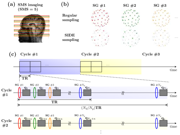
Figure 1: (a) SMS acquistion with a factor of 5. (b) SIDE acquisition with the SMS slice groups covering different gradient directions, unlike conventional sampling. (c) An illustration of the SIDE sequence.

The wavevector $\mathbf{q}$ depends on the length, strength, and orientation of the gradient pulses during the measurement sequence and the diffusion time on the pulse length and separation. For PGSE measurements, for example, $\mathbf{q}=\gamma\delta\mathbf{G}$ and $t=\Delta-(\delta/3)$, where $\gamma$ is the gyromagnetic ratio, $\mathbf{G}$ is the diffusion gradient, $t$ is the diffusion time, $\Delta$ is the time between the onsets of the two pulses, and both pulses have length $\delta$. Often we separate $\mathbf{q}$ into a scalar wavenumber $|\mathbf{q}|$ and a diffusion encoding direction $\hat{\mathbf{q}}=\mathbf{q}/|\mathbf{q}|$, which is the direction of the magnetic field gradient in the diffusion-weighted pulses. The $b$-value summarizes both diffusion time and wavenumber $b=t|\mathbf{q}|^{2}$. For spherical acquisition schemes, both $t$ and $|\mathbf{q}|$ are fixed (so $b$ is fixed) and only the gradient direction varies among measurements. The wavevectors can be computed from the $b$-values and gradient directions listed in the gradient table if the diffusion time is known.

II-B Reconstruction Problem

Our reconstruction method is summarized in Figure 2. For each $n\,=\,1,\cdots,N_{d}$, let $\tilde{X}_{n}$ be the slice stacks reorganized from the SIDE volumes acquired with a factor of $R$ in the slice-select direction. Our objective is to reconstruct the full DW volumes $\{X_{n}\}$ from the undersampled DW volumes $\{\tilde{X}_{n}\}$ by learning a non-linear mapping function $f$ such that

$$(X_{1},\cdots,X_{N_{d}})=f(\tilde{X}_{1},\cdots,\tilde{X}_{N_{d}}).$$ (1)

Instead of reconstructing each DW volume individually, all DW volumes will be simultaneously reconstructed by jointly considering $x$-space and $q$-space neighborhoods. We learn the non-linear mapping function $f$ in (1) using a GCNN. By joint consideration of $x$-space and $q$-space neighborhoods, the complementary information acquired from different DW volumes can be harnessed jointly for effective reconstruction. Note that the input of the GCNN is a graph constructed from the subsampled DW images instead of the fully interpolated images. This reduces computational complexity and memory requirements.

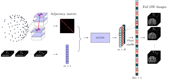
Figure 2: GCNN-based reconstruction framework.

II-C Graph Representation

We represent the dMRI signal as a function defined on the nodes of a graph, where each node is determined by a physical spatial location in $x$-space and a wavevector in $q$-space. This graph is encoded with a weighted adjacency matrix $W$, which characterizes the relationships between two nodes. The graph Laplacian operator, defined as $L=D-W$ with $D$ being a diagonal degree matrix, plays an important role in graph signal processing. $L$ can be normalized as $L=I-D^{-1/2}WD^{-1/2}$, where $I$ is an identity matrix. As $L$ is real symmetric positive semidefinite, it has a set of orthonormal eigenvectors. The eigenvectors of $L$ define the graph Fourier transform that enables the formulation of filtering in the spectral domain [18]. Construction of the adjacency matrix $W$ will be explained in Section II-E.

II-D Spectral Graph Convolution

Localized graph filters are defined based on spectral graph theory [18]. According to the Parseval’s theorem [19], the spatial localization of the convolution corresponds to the smoothness in the spectral domain [9]. Hence, localized filters can be approximated and parameterized by polynomials [19]. Spectral filters represented by the $K$-th order polynomials of the Laplacian are $K$-hop localized in the graph [20]. In the current work, we employ Chebyshev polynomial approximation and define the graph convolutional operation from input $x$ to output $y$ as

$$y=g_{\theta}(x)=\sum_{k=0}^{K}\theta_{k}T_{k}(\tilde{L})x,$$ (2)

where $T_{k}(\tilde{L})$ is the Chebyshev polynomial of order $k$ evaluated for the scaled Laplacian $\tilde{L}:=2L/\lambda_{\max}-I$ with $\lambda_{\max}$ being the maximal eigenvalue of $L$. Chebyshev polynomials $\{T_{k}(\cdot)\}$ form an orthogonal basis on $[-1,1]$ and can be computed by the stable recurrence relation

$$T_{k}(\lambda)=2\lambda T_{k-1}(\lambda)-T_{k-2}(\lambda),\text{with}~{}T_{0}(\lambda)=1,~{}T_{1}(\lambda)=\lambda.$$ (3)

Then, the graph convolutional layers in the GCNN can be represented as

$$\mathbf{\Phi}^{(l)}=\xi\bigg{(}\sum_{k=0}^{K}{{\Theta}}_{k}^{(l)}T_{k}({\tilde{L}})\mathbf{\Phi}^{(l-1)}\bigg{)},$$ (4)

where $\mathbf{\Phi}^{(l)}$ denotes the feature map at the $l$-th layer, ${\Theta}_{k}^{(l)}$ is a matrix of Chebyshev polynomial coefficients to be learned at the $l$-th layer, and $\xi$ denotes a non-linear activation function.

II-E Adjacency Matrix

We define the adjacency matrix by jointly considering spatio-angular neighborhoods. The dMRI signal sampling domain can be represented as a graph with each node representing a spatial location $\mathbf{x}_{i}\in\mathbb{R}^{3}$ and a normalized wavevector $\hat{\mathbf{q}}_{j}\in\mathbb{S}^{2}$. Inspired by the $x$-$q$ space neighborhood matching strategy for dMRI denoising [21], we define a symmetric adjacency matrix $W$ with weight elements $\{w_{i,j;i^{\prime},j^{\prime}}\}$:

$$w_{i,j;\,i^{\prime},j^{\prime}}{:=}\exp\left(-\frac{\|\mathbf{x}_{i}-\mathbf{x}_{i^{\prime}}\|_{2}^{2}}{\sigma_{x}^{2}}\right)\exp\left(-\frac{1-\langle\hat{\mathbf{q}}_{j},\hat{\mathbf{q}}_{j^{\prime}}\rangle^{2}}{\sigma_{q}^{2}}\right),$$ (5)

where $\sigma_{x}$ and $\sigma_{q}$ are the parameters used to control the contributions from the spatial and angular neighborhoods distances, respectively. We note that the numerators of the arguments of the exponential functions in (5) are normalized to $[0,1]$.

II-F Graph Convolutional Neural Networks

Our generator architecture is based on U-Net [22] with symmetric encoding and decoding paths. In U-Net, encoding and decoding pathways require pooling and unpooling operations, respectively. Graph coarsening and uncoarsening, which correspond to pooling and unpooling in standard CNNs, are not defined as straightforwardly. For graph coarsening, we adopt the Graclus multi-scale clustering algorithm [23] as in [18]. Moreover, a residual convolutional block is employed to ease network training since it can mitigate the problem of vanishing gradients [24]. The graph signal is represented as a single-array vector with permutation indices for rearrangement. The uncoarsening operation is achieved via one-dimensional upsampling operation with a transposed convolution filter [25].

Multi-scale input graphs, generated from graph coarsening, are added as new features with graph convolutions at the encoding path of each level. For skip connection for each level of the encoding path to the decoding path, we apply a transformation module to boost the low-level features to complement the high-level features, as proposed in [26]. Graph convolutions followed by concatenation in the transformation module narrow the gap between low- and high-level features.

The upsampling operation in slice-select direction is realized by standard convolutional layers in the low-resolution space followed by pixel shuffling in the last layer of the network [27]. The pixel-shuffling operation converts $R$ pre-shuffled feature maps of size $m\times 1$ to an output feature map of size $Rm\times 1$, where $m$ is the number of input graph nodes and $R$ is the upsampling factor.

In addition to the reconstruction of full DW images, inspired by [28], we add a branch in the decoding path to compute diffusion indices such as generalized fractional anisotropy (GFA) [29]. This branch can help the generator to produce dMRI data with more accurate diffusion indices. In this work, we focus on only GFA, which is estimated by one graph convolutional layer followed by two consecutive fully-connected layers.

The architecture of our generator is illustrated in Figure 3. The numbers of feature maps are set to 64, 128, and 256 for the respective levels. The last graph convolutional layer in the image reconstruction branch has $R$ channels with pre-shuffled feature maps for pixel shuffling.

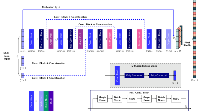
Figure 3: The proposed graph CNN architecture. For each convolution layer, $K$ corresponds to Chebyshev polynomial order and $F$ corresponds to the number of feature maps.

II-G Adversarial Learning

We employ adversarial learning to generate more realistic image outputs. In adversarial learning, the generator attempts to produce outputs that cannot be distinguished from the target images by an adversarially trained discriminator [14]. The training of the generator and the discriminator is performed in an alternating fashion. Here, the generator is the proposed GCNN with two output branches as shown in Figure 3. We apply two separate discriminators for the predicted DW image and the predicted diffusion index. That is, a discriminator $D_{I}$ that classifies between the predicted DW image and the real DW image, and another discriminator $D_{\text{GFA}}$ that classifies between the predicted GFA image and the real GFA image. We use leaky ReLU (LReLU) activation for both discriminators with negative slope 0.2, as suggested in [12] for stable GANs.

For the input source $\mathbf{x}$, the target DW image $\mathbf{y}_{I}$, and the target GFA $\mathbf{y}_{\text{GFA}}$ , the generator loss is defined as the combination of pixel-wise difference, GFA difference, and adversarial loss:

$$\mathcal{L}_{G}(\mathbf{x},\mathbf{y}_{I},\mathbf{y}_{\text{GFA}})$$

$$= \lambda_{I}\|G_{I}(\mathbf{x})-\mathbf{y}_{I}\|_{1}+\lambda_{\text{GFA}}\|G_{\text{GFA}}(\mathbf{x})-\mathbf{y}_{\text{GFA}}\|_{1}$$

$$+ \lambda_{\text{ADV}}(\mathcal{L}_{\text{BCE}}(D_{I}(G_{I}(\mathbf{x})),\mathbf{1})+\mathcal{L}_{\text{BCE}}(D_{\text{GFA}}(G_{\text{GFA}}(\mathbf{x})),\mathbf{1})),$$

where $\mathcal{L}_{\text{BCE}}$ is the binary cross-entropy function, and $D_{I}$ and $D_{\text{GFA}}$ are the discriminators for the predicted images and GFA, respectively. In (II-G), $G_{I}(\mathbf{x})$ and $G_{\text{GFA}}(\mathbf{x})$ are the outputs of the generator in the image reconstruction branch and diffusion index branch, respectively. We define the discriminator loss as

$$\mathcal{L}_{D_{I}}(\mathbf{x},\mathbf{y}_{I}) = \mathcal{L}_{\text{BCE}}(D_{I}(\mathbf{y}_{I}),\mathbf{1})+\mathcal{L}_{\text{BCE}}(D_{I}(G_{I}(\mathbf{x})),\mathbf{0}),$$

$$\mathcal{L}_{D_{\text{GFA}}}(\mathbf{x},\mathbf{y}_{\text{GFA}}) = \mathcal{L}_{\text{BCE}}(D_{\text{GFA}}(\mathbf{y}_{\text{GFA}}),\mathbf{1})$$

$$+ \mathcal{L}_{\text{BCE}}(D_{\text{GFA}}(G_{\text{GFA}}(\mathbf{x})),\mathbf{0}).$$

$D_{I}$ consists of three graph convolutions with 64, 128, 256 features, each followed by LReLU and graph pooling. $D_{\text{GFA}}$ consists of three fully-connected layers with 64, 32, and 1 node(s), respectively.

III Experimental Results

The proposed method is validated with retrospectively undersampled HCP data and in vivo human brain data acquired with SIDE.

III-A Materials

III-A1 Simulated Data

We demonstrate the effectiveness of our method using randomly selected 16 subjects from the Human Connectome Project (HCP) database [30]. We perform 4-fold cross-validation with 12 subjects for training and 4 subjects for testing at each fold. Each subject has a total of 270 DW images of voxel size $1.25^{3}\,\text{mm}^{3}$, 90 each for $b=1000,\,2000,\,3000\,\text{s/mm}^{2}$. We retrospectively undersampled the images by factors $R=3,4,5$ and $6$. Specifically, the set of DW images was divided into $R$ subsets so that the wavevectors were uniformly distributed in each subset. For each subset, the source images were generated by undersampling the original images with a slice offset. For each undersampling factor $R$, we extract input and output patches with size $R\times R\times 1\times 90$ and $R\times R\times R\times 90$, respectively. In order to harness more contextual information to recover missing slices, the patch size increases with the undersampling factor $R$.

III-A2 SIDE Data

After obtaining informed consent, we acquired dMRI data from seven healthy subjects using a protocol approved by the institute and a 3T Siemens whole-body Prisma scanner (Siemens Healthcare, Erlangen, Germany). Diffusion imaging was performed with a monopolar diffusion-weighted PGSE-EPI sequence. The SMS RF excitation with controlled aliasing (blipped-CAIPI) was employed to reduce the penalty of geometry factor (g-factor). The SMS factor is 5. Imaging parameters were as follows: resolution= $1.5^{3}\,\text{mm}^{3}$; FOV $=192\times 192\times 150\,\text{mm}^{3}$; image dimensions $=128\times 128\times 100$; partial Fourier = 6/8; no in-plane acceleration was used; bandwidth = 1776 Hz/Px; 160 wavevectors distributed over the 4 b-shells of $b=500,1000,2000$, and $3000\,\text{s/mm}^{2}$ with 16, 32, 48, and 64 non-collinear directions respectively, plus one $b=0\,\text{s/mm}^{2}$ scan; TR/TE$~{}=~{}3120/90$ ms; 32-channel head array coil. The total acquisition time for full DW images is 8 mins and 19 secs for each phase-encoding direction. Note that $N_{d}=160$ and $N_{g}=100/5=20$. SG is shifted by $\kappa=1$ for each cycle.

We performed leave-one-out cross-validation for 48 DW images ($b=2000\,\text{s/mm}^{2}$) with undersampling factors $R=2,4,$ and $10$. For each undersampling factor $R$, we extract input and output patches with size $5\times 5\times 1\times 48$ and $5\times 5\times R\times 48$, respectively. For $R=2$, we selected the 1st to 10th cycles from 20 cycles. For $R=4$, we selected the 1st, 3rd, 5th, 7th, and 9th cycles. For $R=10$, we selected the 1st and 16th cycles. The ground truth full DW images were acquired with all 20 cycles.

III-B Implementation Details

All DW images were normalized by their respective non-DW image ($b_{0}$). The weight controlling parameters in (5) are set to $\sigma_{x}^{2}=0.1$ and $\sigma_{q}^{2}=1.0$ for joint consideration of spatial and angular distances. The order of the Chebyshev polynomials $K$ is set to $3$. For the loss functions, we set $\lambda_{I}=1.0$, $\lambda_{\text{GFA}}=0.1$, and $\lambda_{\text{ADV}}=0.01$. The proposed method was implemented using TensorFlow 1.13.1 and trained with the ADAM optimizer with an initial learning rate of 1$\times$10^-4 and 1$\times$10^-5 for the generator and the discriminators, respectively, and a mini-batch size of 10. The learning rate is decreased with an exponential decay rate of 0.95 at every 10,000 steps.

III-C Results

III-C1 Simulated Data

We compared our method (with and without GFA loss) with bicubic interpolation and 3D U-Net [31] applied to input images upsampled via bicubic interpolation, for four different undersampling factors and three different b-shells. For 3D U-Net, we extracted patches of size $16\times 16\times 16$ with patch offset $8$. We also implemented a GCNN method which is applied to the patches extracted from the upsampled inputs by bicubic interpolation as in 3D U-Net. This Bicubic+GCNN is essentially the same as the proposed method except the last pixel-shuffling layer. The patch size was fixed as $4\times 4\times 4\times 90$ with patch offset $3$ for the Bicubic+GCNN for all $R$’s. For our method, we set the input and output patch sizes as $R\times R\times 1\times 90$ and $R\times R\times R\times 90$, respectively. Table I gives the number of training parameters of the generator for $R=4$. Note that the number of channels in Bicubic+GCNN was set to 64 for all layers so that the number of parameters was comparable to the other methods.

TABLE I: Number of training parameters ($R=4$).

Bicubic+3D U-Net	Bicubic+GCNN	GCNN	GCNN+GFA loss
$5.60\times 10^{6}$	$6.63\times 10^{6}$	$5.37\times 10^{6}$	$5.43\times 10^{6}$

We measure the reconstruction accuracy of DW images by means of mean absolute error (MAE), peak signal-to-noise ratio (PSNR), and structural similarity index (SSIM). We also computed the GFA maps of the reconstructed DW images. The quantitative results under the different undersampling factors at fixed $b\,=\,2000\,\text{s/mm}^{2}$ are summarized in Figure 4 for DW images and in Figure 5 for GFA maps. We also compared the proposed method for different b-values at $R=4$ and the results are summarized in Figure 6. The quantitative results demonstrate that GCNN is superior to 3D U-Net as it exploits angular neighborhood information in the form of graphs. Our method yields results that are better than Bicubic+GCNN, since Bicubic+GCNN uses fixed hand-crafted upsampling, whereas our method learns the upsampling mapping via the pixel-shuffling operation. Moreover, our method is faster than Bicubic+GCNN with lower computational cost. The results in Figures 4, 5 and 6 indicate that the improvements over other competing methods are statistically significant ($p<0.01$, Wilcoxon signed-rank test).

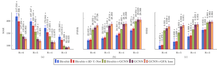
Figure 4: Quantitative comparison of DW images using (a) MAE, (b) PSNR, and (c) SSIM, under different undersampling factors. $\ast$ and $\dagger$ indicate the $p$-value $<0.01$ and $<0.05$, respectively, compared to GCNN+GFA loss.

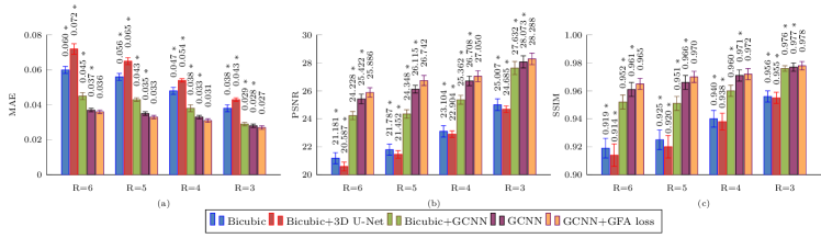
Figure 5: Quantitative comparison of GFA using (a) MAE, (b) PSNR, and (c) SSIM, under different undersampling factors. $\ast$ and $\dagger$ indicate the $p$-value $<0.01$ and $<0.05$, respectively, compared to GCNN+GFA loss.

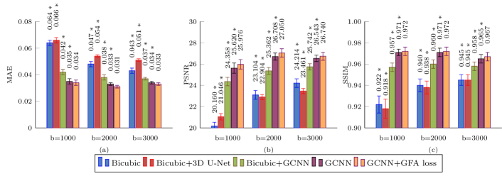
Figure 6: Quantitative comparison of GFA using (a) MAE, (b) PSNR, and (c) SSIM, under different shells. $\ast$ and $\dagger$ indicate the $p$-value $<0.01$ and $<0.05$, respectively, compared to GCNN+GFA loss.

Representative reconstruction results for GFA at $R=5$ and $b=2000\,\text{s/mm}^{2}$, shown in Figure 7, indicate that the proposed methods recover more structural details compared with the competing methods. Moreover, the error in slice-select direction is significantly reduced when GFA loss is considered. Figure 8 shows root-mean-square-error (RMSE) map of spherical harmonic (SH) coefficients of maximum order 8.

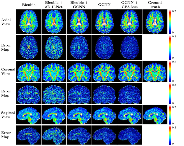
Figure 7: Computed GFA maps from the predicted DW images and the corresponding error maps shown in multiple views ($R=5,b=2000$).

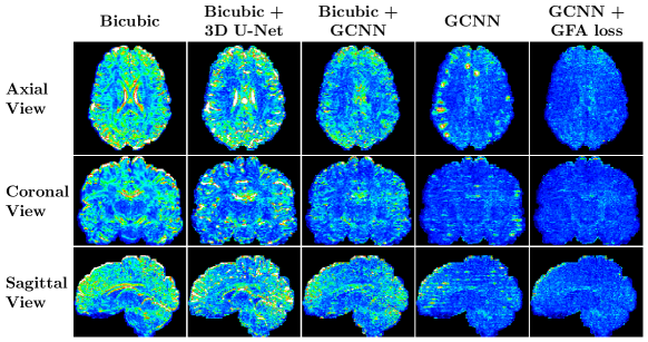
Figure 8: RMSE of SH coefficients shown in multiple views with display window $[0,300]$ ($R=5,b=2000$).

Evaluation was also performed based on the diffusion indices given by neurite orientation dispersion and density imaging (NODDI) [32], applied on multi-shell data with each shell predicted using the different methods. The quantitative results for intra-cellular volume fraction (ICVF), isotropic volume fraction (ISOVF), and orientation dispersion (OD) are summarized in Figure 9. A representative result of ICVF for $R=4$ is shown in Figure 10. While either the bicubic interpolation or the results learned from fixed interpolated source are blurry, our method yields results that are relatively sharp and closer to the ground truth. Moreover, the error shown in slice-select direction is significantly reduced with GFA loss.

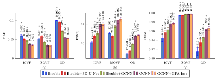
Figure 9: Quantitative comparison of the measures of NODDI models using (a) MAE, (b) PSNR, and (c) SSIM. $\ast$ and $\dagger$ indicate $p<0.01$ and $p<0.05$, respectively, compared to GCNN+GFA loss.

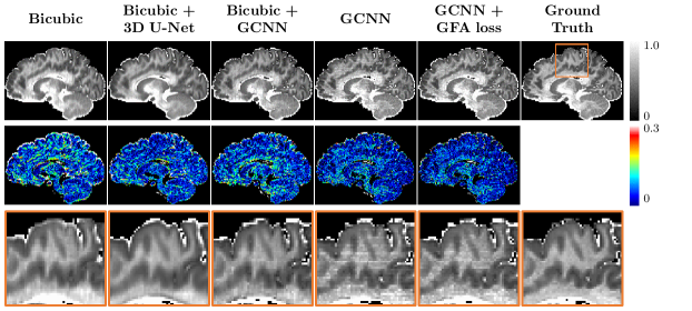
Figure 10: Representative ICVF maps (top row), the corresponding error maps (middle row), and their close-up views (bottom row).

Figure 11 shows that our method provides more coherent and accurate fiber orientation distribution functions (ODFs) with less partial volume effects, especially in the regions marked by the rectangles.

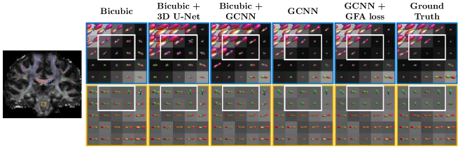
Figure 11: Representative fiber ODFs ($R=4$).

III-C2 SIDE Data

We also evaluated our method with the SIDE data of seven subjects for $b\,=\,2000\,\text{s/mm}^{2}$ under various acceleration factors $R\,=\,2,\,4$, and $10$. The patch sizes for 3D U-Net and Bicubic+GCNN were set to be the same as the simulated data. The quantitative results for the different undersampling factors are summarized in Figure 12 for GFA maps, again demonstrating that our method is superior to the methods exploiting only spatial neighborhood information. Note that for $R\,=\,2$, the difference between our method and other competing methods are marginal. However, the improvement becomes more significant as the undersampling factor increases. Representative reconstruction results for GFA at $R=4$, shown in Figure 13, confirm that the proposed methods recover more structural details, especially in the body of corpus callosum and near the cerebral cortex, compared with the competing methods.

Note that we selected certain cycles out of 20 cycles for different undersampling factors so that the acquired slices for each wavevector are as equally-spaced as possible. For the HCP simulated data, the undersampled slices were exactly equally-spaced.

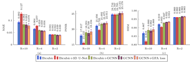
Figure 12: Quantitative comparison of GFA using (a) MAE, (b) PSNR, and (c) SSIM, under different undersampling factors.

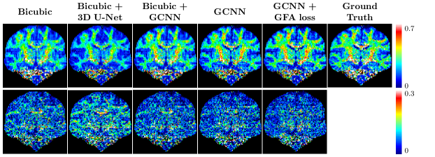
Figure 13: Computed GFA maps from the predicted DW images and the corresponding error maps shown in coronal views ($R=4$).

IV Discussion

We have shown that the proposed GCNN is capable of recovering DW images from highly undersampled data acquired via SIDE with acceleration factor as high as 10 (50 with SMS acquisition). We will discuss here some limitations of the proposed framework and future work for improvements.

Gradient ordering throughout the cycles needs to be further optimized. Currently, gradient ordering is varied at each cycle by offsetting the gradient table with a step of 1. This is not necessarily optimal and causes the slices acquired in two consecutive cycles to be highly correlated. That is, adjacent slices for each gradient are acquired as the cycle progresses. A more optimal ordering strategy should ensure that incoherent information is covered across cycles. Incoherence in general promotes more effective recovery of unsampled information.

The proposed reconstruction framework assumes a consistent gradient table in training and testing, preventing the learned mapping to be applied to data collected using different gradient tables. This limitation can be overcome by utilizing GCNN methods that are based on heterogeneous graphs [33]. Another potential solution is to learn the mappings between representations, such as spherical harmonics (SHs), instead of the signal directly. That is, the mapping between the SHs of the undersampled data to the SHs of fully-sampled data can be learned and applied to data collected with different numbers of gradient directions as long as the signal is consistently represented by SHs up to a fixed maximum order.

Conventional dMRI acquisition typically covers the slices associated with each diffusion gradient fully before proceeding with the next gradient. In contrast, SIDE acquisition covers the slice groups of all gradients in each cycle and repeats in the next cycle with a gradient offset (see Figure 1c). In other words, each cycle covers partial information of all gradients. This is the key characteristic of SIDE that allows unsampled information to be recovered from the data acquired in a few cycles.

The above observation has important implications on scan disruption caused for example by subject motion. In conventional dMRI acquisition, disruption results in the total loss of information with respect to some diffusion gradients, which can be challenging to recover. On the other hand, disruption of SIDE acquisition results in partial loss of slices of a volume. The lost slices can be recovered from adjacent slices acquired with the same and similar gradients.

SIDE acquisition can potentially improve post-acquisition motion correction, for example, by registering motion-affected data to motion-free data. If SIDE acquisition is able to complete motion-free for a few cycles, the acquired data, which cover all gradients, can be used as a reference for registration-based motion correction. Alternatively, a reference for registration-based correction can be constructed by generating the full data using the motion-free data using our reconstruction framework.

The time saved by using SIDE acquisition can be used for a denser coverage of the $q$-space, which in turn also improves reconstruction based on the SIDE data since more information in the $q$-space can be leveraged for data prediction. This opens the opportunity for dense $q$-space coverage to allow for better prediction of tissue microstructure and white matter pathways. The balance between $q$-space coverage and $x$-space coverage in terms of slices is a subject of future research.

V Conclusion

We have proposed a novel slice-based sampling technique to accelerate dMRI acquisition. The slices in a volume are encoded with multiple diffusion gradients to allow for rapid sampling of information associated with different gradients. Highly subsampled data acquired using this approach can then be fed into a deep learning framework that jointly considers spatial and wavevector domains to reconstruct the full data. The high acceleration factor achievable opens the door to future opportunities for improved motion correction and dense $q$-space imaging.

References

- [1] T. E. Behrens and H. Johansen-Berg, Diffusion MRI: From quantitative measurement to in-vivo neuroanatomy. Academic Press, 2009.
- [2] L. Ning, K. Setsompop, O. Michailovich, N. Makris, M. E. Shenton, C.-F. Westin, and Y. Rathi, “A joint compressed-sensing and super-resolution approach for very high-resolution diffusion imaging,” NeuroImage, vol. 125, pp. 386–400, 2016.
- [3] G. Chen, B. Dong, Y. Zhang, W. Lin, D. Shen, and P.-T. Yap, “Angular upsampling in infant diffusion mri using neighborhood matching in xq space,” Frontiers in Neuroinformatics, vol. 12, p. 57, 2018.
- [4] J. Cheng, D. Shen, P. J. Basser, and P.-T. Yap, “Joint 6D kq space compressed sensing for accelerated high angular resolution diffusion MRI,” in International Conference on Information Processing in Medical Imaging. Springer, 2015, pp. 782–793.
- [5] M. Mani, M. Jacob, A. Guidon, V. Magnotta, and J. Zhong, “Acceleration of high angular and spatial resolution diffusion imaging using compressed sensing with multichannel spiral data,” Magnetic resonance in medicine, vol. 73, no. 1, pp. 126–138, 2015.
- [6] W. Wu, P. J. Koopmans, J. L. Andersson, and K. L. Miller, “Diffusion acceleration with gaussian process estimated reconstruction (DAGER),” Magnetic resonance in medicine, vol. 82, no. 1, pp. 107–125, 2019.
- [7] F. Shi, J. Cheng, L. Wang, P.-T. Yap, and D. Shen, “Super-resolution reconstruction of diffusion-weighted images using 4D low-rank and total variation,” in MICCAI Workshop on Computational Diffusion MRI. Springer, 2016, pp. 15–25.
- [8] R. Tanno, D. E. Worrall, A. Ghosh, E. Kaden, S. N. Sotiropoulos, A. Criminisi, and D. C. Alexander, “Bayesian image quality transfer with CNNs: exploring uncertainty in dMRI super-resolution,” in Medical Image Computing and Computer-Assisted Intervention (MICCAI). Springer, 2017, pp. 611–619.
- [9] J. Bruna, W. Zaremba, A. Szlam, and Y. LeCun, “Spectral networks and locally connected networks on graphs,” arXiv preprint arXiv:1312.6203, 2013.
- [10] M. Henaff, J. Bruna, and Y. LeCun, “Deep convolutional networks on graph-structured data,” arXiv preprint arXiv:1506.05163, 2015.
- [11] I. Goodfellow, J. Pouget-Abadie, M. Mirza, B. Xu, D. Warde-Farley, S. Ozair, A. Courville, and Y. Bengio, “Generative adversarial nets,” in Advances in Neural Information Processing Systems (NIPS), 2014, pp. 2672–2680.
- [12] A. Radford, L. Metz, and S. Chintala, “Unsupervised representation learning with deep convolutional generative adversarial networks,” arXiv preprint arXiv:1511.06434, 2015.
- [13] E. L. Denton, S. Chintala, R. Fergus et al., “Deep generative image models using a laplacian pyramid of adversarial networks,” in Advances in Neural Information Processing Systems (NIPS), 2015, pp. 1486–1494.
- [14] P. Isola, J.-Y. Zhu, T. Zhou, and A. A. Efros, “Image-to-image translation with conditional adversarial networks,” arXiv preprint, 2017.
- [15] J.-Y. Zhu, T. Park, P. Isola, and A. A. Efros, “Unpaired image-to-image translation using cycle-consistent adversarial networks,” arXiv preprint, 2017.
- [16] Y. Hong, G. Chen, P.-T. Yap, and D. Shen, “Multifold acceleration of diffusion MRI via deep learning reconstruction from slice-undersampled data,” in International Conference on Information Processing in Medical Imaging. Springer, 2019, pp. 530–541.
- [17] ——, “Reconstructing high-quality diffusion MRI data from orthogonal slice-undersampled data using graph convolutional neural networks,” in International Conference on Medical Image Computing and Computer-Assisted Intervention. Springer, 2019, pp. 529–537.
- [18] M. Defferrard, X. Bresson, and P. Vandergheynst, “Convolutional neural networks on graphs with fast localized spectral filtering,” in Advances in Neural Information Processing Systems (NIPS), 2016, pp. 3844–3852.
- [19] M. M. Bronstein, J. Bruna, Y. LeCun, A. Szlam, and P. Vandergheynst, “Geometric deep learning: going beyond Euclidean data,” IEEE Signal Processing Magazine, vol. 34, no. 4, pp. 18–42, 2017.
- [20] D. K. Hammond, P. Vandergheynst, and R. Gribonval, “Wavelets on graphs via spectral graph theory,” Applied and Computational Harmonic Analysis, vol. 30, no. 2, pp. 129–150, 2011.
- [21] G. Chen, B. Dong, Y. Zhang, D. Shen, and P.-T. Yap, “Neighborhood matching for curved domains with application to denoising in diffusion MRI,” in Medical Image Computing and Computer-Assisted Intervention (MICCAI). Springer, 2017, pp. 629–637.
- [22] O. Ronneberger, P. Fischer, and T. Brox, “U-net: Convolutional networks for biomedical image segmentation,” in International Conference on Medical image computing and computer-assisted intervention. Springer, 2015, pp. 234–241.
- [23] I. S. Dhillon, Y. Guan, and B. Kulis, “Weighted graph cuts without eigenvectors a multilevel approach,” IEEE transactions on pattern analysis and machine intelligence, vol. 29, no. 11, pp. 1944–1957, 2007.
- [24] K. He, X. Zhang, S. Ren, and J. Sun, “Deep residual learning for image recognition,” in Computer Vision and Pattern Recognition (CVPR), 2016, pp. 770–778.
- [25] J. Long, E. Shelhamer, and T. Darrell, “Fully convolutional networks for semantic segmentation,” in Computer Vision and Pattern Recognition (CVPR), 2015, pp. 3431–3440.
- [26] D. Nie, L. Wang, E. Adeli, C. Lao, W. Lin, and D. Shen, “3-D fully convolutional networks for multimodal isointense infant brain image segmentation,” IEEE Transactions on Cybernetics, 2018.
- [27] W. Shi, J. Caballero, F. Huszár, J. Totz, A. P. Aitken, R. Bishop, D. Rueckert, and Z. Wang, “Real-time single image and video super-resolution using an efficient sub-pixel convolutional neural network,” in Computer Vision and Pattern Recognition (CVPR), 2016, pp. 1874–1883.
- [28] G. Chen, Y. Hong, K. Huynh, W. Lin, D. Shen, and P.-T. Yap, “Prediction of multi-shell diffusion MRI data using deep neural networks with diffusion loss,” 105th RSNA Scientific Assembly and Annual Meeting, 2019.
- [29] D. S. Tuch, “Q-ball imaging,” Magnetic Resonance in Medicine, vol. 52, no. 6, pp. 1358–1372, 2004.
- [30] S. N. Sotiropoulos, S. Jbabdi, J. Xu, J. L. Andersson, S. Moeller, E. J. Auerbach, M. F. Glasser, M. Hernandez, G. Sapiro, M. Jenkinson et al., “Advances in diffusion MRI acquisition and processing in the human connectome project,” NeuroImage, vol. 80, pp. 125–143, 2013.
- [31] Ö. Çiçek, A. Abdulkadir, S. S. Lienkamp, T. Brox, and O. Ronneberger, “3D U-Net: learning dense volumetric segmentation from sparse annotation,” in Medical Image Computing and Computer-Assisted Intervention (MICCAI). Springer, 2016, pp. 424–432.
- [32] H. Zhang, T. Schneider, C. A. Wheeler-Kingshott, and D. C. Alexander, “NODDI: practical in vivo neurite orientation dispersion and density imaging of the human brain,” Neuroimage, vol. 61, no. 4, pp. 1000–1016, 2012.
- [33] F. P. Such, S. Sah, M. A. Dominguez, S. Pillai, C. Zhang, A. Michael, N. D. Cahill, and R. Ptucha, “Robust spatial filtering with graph convolutional neural networks,” IEEE Journal of Selected Topics in Signal Processing, vol. 11, no. 6, pp. 884–896, 2017.