A Lyapunov Approach to Barrier-Function Based Time-Varying Gains Higher Order Sliding Mode Controllers

Abstract

In this paper, we present Lyapunov-based time varying controllers for fast stabilization of a perturbed chain of integrators with bounded uncertainties. We refer to such controllers as time varying higher order sliding mode controllers since they are designed for nonlinear Single-Input-Single-Output (SISO) systems with bounded uncertainties such that the uncertainty bounds are unknown. We provide a time varying control feedback law insuring verifying the following: there exists a family $\displaystyle(D(t))_{t\geq 0}$ of time varying open sets decreasing to the origin as $\displaystyle t$ tends to infinity, such that, for any unknown uncertainty bounds and trajectory $\displaystyle z(\cdot)$ of the corresponding system, there exists a positive positve $\displaystyle t_{z}$ for which $\displaystyle z(t_{z})\in D(t_{z})$ and $\displaystyle z(t)\in D(t)$ for $\displaystyle t\geq t_{z}$. The effectiveness of these controllers is illustrated through simulations.

1 Introduction

Sliding Mode Control is an efficient tool for matched uncertainties compensation. Higher Order Sliding Mode Controllers (HOSMCs) [1, 2, 3, 4, 5, 6] allow to reduce the dynamics of systems of order $\displaystyle n$ with relative degree $\displaystyle r$ till $\displaystyle(n-r)$. The homogeneity properties of HOSMCs ensure the $\displaystyle r$-th order of asymptotic precision with respect to the sampling step and parasitic dynamics [1, 2, 3, 7]. To implement HOSMCs, the knowledge of upper bounds for $\displaystyle r$-th derivatives is needed.

In majority of real systems with relative degree $\displaystyle r$, the upper bounds of $\displaystyle r$-th derivatives of the outputs exist but they are unknown [8, 9, 10, 11, 12, 13, 14, 15, 16, 17, 18, 19, 20, 21]. So adaptive HOSMCs design should satisfy two contradictory requirements:

• ensure a finite-time exact convergence to the origin;

• avoid overestimation of the control gain [8].

Recently, adaptive sliding mode controllers have attracted the interest of many researchers dealing with these requirements [22, 9, 10]. For example, in [23, 11, 12] adaptive approaches which are based on the Utkin’s concept of equivalent control have proposed to adapt first order, second order and HOSMC algorithms. However, the realization of this concept requires the knowledge of the equivalent control signal recovered from the filtration of the discontinuous control signal. It is possible to have this information if and only if the upper bound of the perturbations derivative is known. In this case, it is more useful to use continuous HOSMC. Inspired by this concept, an adaptive strategy has proposed in [13] for first order sliding mode control. The advantages of this strategy are its simplicity and the possibility to be implemented in the case of non smooth perturbations. Furthermore, with the aim of making less restrictive assumptions on the class of perturbations as well as maitaining the sliding mode, a monitoring function-based adaptive approach is proposed for first order sliding mode control in [14].

On the other hand, another common approach which used dynamic gain adaptation is introduced by Huang et al. [24] for first order sliding mode control. In this adaptation, the control gain increases until the sliding mode is achieved, and afterwards the gain becomes constant and stabilizes at unnecessarily large value. Inspired by this adaptation, Moreno et al. [15, 10] have proposed an adaptation of different HOSMC algorithms that has the same aforementioned problem. Plestan et al. [8, 25] have overcome this problem by decreasing the gains once the sliding mode is achieved. This method establishes real-sliding mode (convergence to a neighborhood of the sliding surface). However, it does not guarantee that the sliding variable would remain inside the neighborhood after convergence. In the field of HOSMC, Shtessel et al. [16, 17] used this method to adapt super-twisting and twisting algorithms with non-overestimation of the control gains. In both algorithms, the sliding variable and its first time derivative converge to some unknown neighborhoods of zero.

Unlike these previous approaches, a barrier function-based adaptive strategy is proposed to overcome the problem of unknow domain of convergence [18]. Indeed, this strategy has been applied to adapt a first order sliding mode and super-twisting algorithms and it ensures the convergence of the output variable and maintains it in a predefined neighborhood of zero independent of the upper bounds of the perturbation and its derivative, without overestimating the control gain [18, 26, 27]. Inspired by this strategy, an adaptive twisting algorithm ensuring the convergence of the sliding variable and its first time derivative to some predefined neighborhoods of zero is presented in [28]. As a generalization of the results presented in [26], an adaptive integral sliding mode control is designed in [29] for a perturbed chain of integrators. This algorithm provides the convergence of the sliding variable and its $\displaystyle r-1$ first derivatives to some unknown neighborhoods of zero. To deal with this drawback, a barrier function-based dual layer strategy which can ensure the convergence of the sliding variable and its $\displaystyle r-1$ first derivatives to zero is proposed in [30]. However, the two drawbacks of this strategy are that, on one hand, it cannot be applied in the case of time-dependent control gain, and on the other hand, the convergence can be lost if the perturbation grows suddenly, this means, the states can leave the origin and jump to a unknown big value before re-convergence.

In this paper, we present Lyapunov-based time varying controllers for the finite time stabilization of a perturbed chain of integrators with bounded uncertainties. Through a minor extension of the definition (as explained in the next section), we refer to such controllers as time varying HOSMCs. The proposed time varying controller guarantees the asymptotic convergence to the origin i.e., it establishes real HOSM. Indeed, it ensures the convergence of the states and their maintenance in a decreasing domain which tends to zero. The main features of such time varying controller can be summarized as follows:

• This controller can be extended to arbitrary order.

• The sliding variable and its $\displaystyle(r-1)$ first derivatives converge in finite time to a family of time varying open sets $\displaystyle(D(t))_{t\geq 0}$ decreasing to the origin as $\displaystyle t$ tends to infinity.

• Once a trajectory enters some $\displaystyle D(t_{*})$ at time $\displaystyle t_{*}$, it remains trapped in the $\displaystyle D(t)$’s, i.e., $\displaystyle z(t)\in D(t)$ for $\displaystyle t\geq t_{*}$.

• The decrease to the origin of the family $\displaystyle(D(t))_{t\geq 0}$ can be chosen arbitrarily.

• We provide an explicit bound on the control which is best possible, i.e., (essentially) linear with respect to the uncertainty.

The paper is organized as follows: problem formulation and time varying controllers are presented in Section 2, simulation results which show the effectiveness of the proposed controllers are presented and discussed in Section 3. Some concluding remarks are given in Section 4.

2 Higher Order Sliding Mode Controllers

If $\displaystyle r$ is a positive integer, the perturbed chain of integrators of length $\displaystyle r$ corresponds to the (uncertain) control system given by

$$\begin{array}[]{lcl}{\color[rgb]{0,0,0}\dot{z}_{i}=z_{i+1},~{}i=1,...,{r-1},}\quad\dot{z}_{r}=\varphi(t)+\gamma(t)u,\end{array}$$ (1)

where $\displaystyle z=[z_{1}\ z_{2}\ ...z_{r}]^{T}\in\mathbb{R}^{r}$, $\displaystyle u\in\mathbb{R}$ and the functions $\displaystyle\varphi$ and $\displaystyle\gamma$ are any measurable functions defined almost everywhere (a.e. for short) on $\displaystyle\mathbb{R}_{+}$ and bounded by positive constants $\displaystyle\bar{\varphi}$, $\displaystyle\gamma_{m}$ and $\displaystyle\gamma_{M}$, such that, for a.e. $\displaystyle t\geq 0$,

$$\begin{array}[]{lcl}\left|\varphi(t)\right|\leq\bar{\varphi},\quad 0<\gamma_{m}\leq\gamma(t)\leq\gamma_{M}.\end{array}$$ (2)

One can equivalently define a perturbed chain of integrators of length $\displaystyle r$ as the differential inclusion $\displaystyle\dot{z}_{r}\in I_{\bar{\varphi}}+uI_{\gamma}$ where $\displaystyle I_{\bar{\varphi}}=\left[-\bar{\varphi},\bar{\varphi}\right]$ and $\displaystyle I_{\gamma}=\left[\gamma_{m},\gamma_{M}\right]$.

The usual objective regarding System (1) consists of stabilizing it with respect to the origin in finite time, i.e., determining feedback laws $\displaystyle u=U(z)$ so that the trajectories of the corresponding closed-loop system converge to the origin in finite time. Note that, in general, the controllers $\displaystyle U(\cdot)$ are discontinuous and then, solutions of (1) need to be understood here in Filippov’s sense [31], i.e., the right-hand vector set is enlarged at the discontinuity points of the differential inclusion to the convex hull of the set of velocity vectors obtained by approaching $\displaystyle z$ from all directions in $\displaystyle\mathbb{R}^{r}$, while avoiding zero-measure sets. Several solutions for this problem exist [1, 2, 3, 4, 5]. under the hypothesis that the bounds $\displaystyle\gamma_{m},\gamma_{M}$ and $\displaystyle\bar{\varphi}$ are known.

In case the bounds $\displaystyle\gamma_{m},\gamma_{M}$ and $\displaystyle\bar{\varphi}$ are unknown (one only assumes their existence) then it is obvious to see that finite time stabilization is not possible by a mere state feedback and therefore, one possible alternate objective consists in achieving asymptotic stabilization. This is the goal of this paper to establish such a result for System (1) and we provide next a precise definition of asymptotic stabilization.

Definition 1.

If $\displaystyle r,p$ are positive integers and $\displaystyle f:\mathbb{R}^{r}\times\mathbb{R}^{p}\rightrightarrows\mathbb{R}^{r}$ is a continuous differential equation, we say that the system $\displaystyle\dot{z}=f(z,u)$ is asymptotic stabilizable if, there exists a continuous controller $\displaystyle u=U(\cdot,t)$ such that every trajectory of the closed-loop system $\displaystyle\dot{z}=f(z,U(\cdot,t))$ tends to the origin as $\displaystyle t$ tends to infinity.

The main result of that paper consists of designing controllers which asymptotically stabilize System (1) independently of the positive bounds $\displaystyle\bar{\varphi}$, $\displaystyle\gamma_{m}$ and $\displaystyle\gamma_{M}$, i.e., the controllers $\displaystyle u=U(\cdot,t)$ which asymptotically stabilize System (1) does not depend on the bounds $\displaystyle\bar{\varphi}$, $\displaystyle\gamma_{m}$ and $\displaystyle\gamma_{M}$.

We next recall the following definition needed in the sequel.

Definition 2.

(Homogeneity. cf. [32].) If $\displaystyle r,m$ are positive integers, a function $\displaystyle f:\mathbb{R}^{r}\rightarrow\mathbb{R}^{m}$ (or a differential inclusion $\displaystyle F:\mathbb{R}^{r}\rightrightarrows\mathbb{R}^{m}$ respectively) is said to be homogeneous of degree $\displaystyle q\in\mathbb{R}$ with respect to the family of dilations $\displaystyle\delta_{\varepsilon}(z)$, $\displaystyle\varepsilon>0$, defined by

$$\delta_{\varepsilon}(z)=(z_{1},\cdots,z_{r})\mapsto(\varepsilon^{p_{1}}z_{1},\cdots,\varepsilon^{p_{r}}z_{r}),$$

where $\displaystyle p_{1},\cdots,p_{r}$ are positive real numbers (the weights), if for every positive $\displaystyle\varepsilon$ and $\displaystyle z\in\mathbb{R}^{r}$, one has $\displaystyle f(\delta_{\varepsilon}(z))=\varepsilon^{q}f(z)$ $\displaystyle\big{(}F(\delta_{\varepsilon}(z))=\varepsilon^{q}\delta_{\varepsilon}(F(z))\ respectively\big{)}$.

The following notations will be used throughout the paper. We define the function sgn as the multivalued function defined on $\displaystyle\mathbb{R}$ by $\displaystyle\hbox{sgn}(x)=\frac{x}{|x|}$ for $\displaystyle x\neq 0$ and $\displaystyle\hbox{sgn}(0)=[-1,1]$. Similarly, for every $\displaystyle a\geq 0$ and $\displaystyle x\in\mathbb{R}$, we use $\displaystyle\left\lfloor x\right\rceil^{a}$ to denote $\displaystyle\left|x\right|^{a}\hbox{sgn}(x)$. Note that $\displaystyle\left\lfloor\cdot\right\rceil^{a}$ is a continuous function for $\displaystyle a>0$ and of class $\displaystyle C^{1}$ with derivative equal to $\displaystyle a\left|\cdot\right|^{a-1}$ for $\displaystyle a\geq 1$. Moreover, for every positive integer $\displaystyle r$, we use $\displaystyle J_{r}$ to denote the $\displaystyle r$-th Jordan block, i.e., the $\displaystyle r\times r$ matrix whose $\displaystyle(i,j)$-coefficient is equal to $\displaystyle 1$ if $\displaystyle i=j-1$ and zero otherwise. Finally, we use $\displaystyle e_{r}$ to denote the vector of $\displaystyle\mathbb{R}^{r}$ equal to $\displaystyle(0\ \cdots\ 0\ 1)^{T}$.

2.1 Time Varying Higher Order Sliding Mode Controller

We first define the system under study and provide parameters used later on.

Definition 3.

Let $\displaystyle r$ be a positive integer. The $\displaystyle r$-th order chain of integrator $\displaystyle(CI)_{r}$ is the single-input control system given by

$$\begin{array}[]{lcl}(CI)_{r}\ \ \ \dot{z}=J_{r}z+ue_{r},\end{array}$$ (3)

with $\displaystyle z=(z_{1},\cdots,z_{r})^{T}\in\mathbb{R}^{r}$ and $\displaystyle u\in\mathbb{R}$. For $\displaystyle\kappa<0$ and $\displaystyle p>0$ with $\displaystyle p+(r+1)\kappa\in[0,1)$, set $\displaystyle p_{i}:=p+(i-1)\kappa,\ 1\leq i\leq r+2$. For $\displaystyle\varepsilon>0$, let $\displaystyle\delta_{\varepsilon}:\mathbb{R}^{r}\rightarrow\mathbb{R}^{r}$ be the family of dilations associated with $\displaystyle\left(p_{1},\cdots,p_{r}\right)$.

In the spirit of [33], we put forwards geometric conditions on certain stabilizing feedbacks $\displaystyle u_{0}(\cdot)$ for $\displaystyle(CI)_{r}$ and corresponding Lyapunov functions $\displaystyle V$. These conditions will be instrumental for the latter developments.

Our construction of the feedback for practical stabilization relies on the following result.

Assumption 1.

Let $\displaystyle r$ be a positive integer. There exists a feedback law $\displaystyle u_{0}:\mathbb{R}^{r}\rightarrow\mathbb{R}$ homogeneous with respect to $\displaystyle(\delta_{\varepsilon})_{\varepsilon>0}$ such that the closed-loop system $\displaystyle\dot{z}=J_{r}z+u_{0}(z)e_{r}$ is finite time globally asymptotically stable with respect to the origin and the following conditions hold true:

$\displaystyle(i)$

the function $\displaystyle z\mapsto J_{r}z+u_{0}(z)e_{r}$ is homogeneous of degree $\displaystyle\kappa$ with respect to $\displaystyle(\delta_{\varepsilon})_{\varepsilon>0}$ and there exists a continuous positive definite function $\displaystyle V{\color[rgb]{0,0,0}(z)}:\mathbb{R}^{r}\rightarrow\mathbb{R}_{+}$, $\displaystyle C^{1}$ except at the origin, homogeneous of positive degree with respect to $\displaystyle(\delta_{\varepsilon})_{\varepsilon>0}$ such that there exists $\displaystyle c>0$ and $\displaystyle\alpha\in(0,1)$ for which the time derivative of $\displaystyle V{\color[rgb]{0,0,0}(z)}$ along non trivial trajectories of $\displaystyle\dot{z}=J_{r}z+u_{0}(z)e_{r}$ verifies

$$\begin{array}[]{lcl}\dot{V}{\color[rgb]{0,0,0}(z)}\leq-cV{\color[rgb]{0,0,0}(z)}^{\alpha};\end{array}$$ (4)

$\displaystyle(ii)$

the function $\displaystyle z\mapsto u_{0}(z)\frac{\partial V{\color[rgb]{0,0,0}(z)}}{\partial z_{r}}$ is non positive over $\displaystyle\mathbb{R}^{r}$ and, for every non zero $\displaystyle z\in\mathbb{R}^{r}$ verifying $\displaystyle u_{0}(z)=0$, one has $\displaystyle\frac{\partial V{\color[rgb]{0,0,0}(z)}}{\partial z_{r}}=0$. As a consequence function $\displaystyle z\mapsto\hbox{sgn}(u_{0}(z))\frac{\partial V{\color[rgb]{0,0,0}(z)}}{\partial z_{r}}$ is well-defined over $\displaystyle\mathbb{R}^{r}\setminus\{0\}$ and non positive.

Remark 1.

Item $\displaystyle(i)$ of the above proposition is classical, see for instance [34, 35, 36]. Item $\displaystyle(ii)$ considers a geometric condition on controllers verifying Item $\displaystyle(i)$, which was introduced in [33] and used in [37]. This geometric condition is indeed satisfied, for instance by Hong’s controller, see [37] for other examples.

Regarding our problem, we consider, for every $\displaystyle\varepsilon>0$ the following controller:

$$\begin{array}[]{lcl}{\color[rgb]{0,0,0}u}(z,z_{0},t)=g(|u_{0}(z)|)u_{0}(z)+k\,\hbox{sgn}\big{(}u_{0}(z)){\color[rgb]{0,0,0}\hat{\varphi}\big{(}t,V(z_{0})\big{)}},\end{array}$$ (5)

where $\displaystyle u_{0}$ and $\displaystyle V{\color[rgb]{0,0,0}(z)}$ are provided by Assumption 1, $\displaystyle g:\mathbb{R}_{+}\rightarrow\mathbb{R}_{+}^{*}$ is an arbitrary increasing $\displaystyle C^{1}$ function tending to infinity as with $\displaystyle x$ tends to infinity and the time varying function $\displaystyle\hat{\varphi}$ is defined later. To proceed, let us first introduce, for every positive real $\displaystyle\xi$, the function $\displaystyle F_{\xi}$ defined on $\displaystyle[0,\xi)$ by $\displaystyle F_{\xi}(x)=\frac{\xi}{\xi-x}$ for $\displaystyle 0<x<\xi$. Moreover, consider $\displaystyle\eta:\mathbb{R}_{+}\rightarrow\mathbb{R}_{+}^{*}$, a non increasing $\displaystyle C^{1}$ function so that $\displaystyle\eta(0)=\varepsilon>0$ and $\displaystyle-\dot{\eta}\leq M\eta$, where $\displaystyle\varepsilon>0$ and $\displaystyle M\geq 0$ are chosen so that $\displaystyle M\varepsilon^{1-\alpha}<c$. Moreover, we define the following family of time varying domains, for $\displaystyle t\geq 0$,

$$\begin{array}[]{lcl}D(t)=\{z\in\mathbb{R}^{r}\ \mid\ V(z)\leq\eta(t)\}.\end{array}$$ (6)

Assume first that $\displaystyle V(z_{0})\leq\varepsilon/2$. Then $\displaystyle\hat{\varphi}\big{(}t,V(z_{0}))$ is defined as $\displaystyle F_{\eta(t)}(V(z(t)))$ for any trajectory $\displaystyle z(\cdot)$ of System (1) closed-looped by the feedback control law (5) and starting at $\displaystyle z_{0}$, and so, as long as $\displaystyle z(\cdot)$ is defined. (Note that in this case there exists a non trivial interval of existence of such solutions since $\displaystyle F_{\eta}$ is continuous.) In case $\displaystyle V(z_{0})>\varepsilon/2$, then $\displaystyle\hat{\varphi}\big{(}t,V(z_{0}))=t$ as long as any trajectory $\displaystyle z(\cdot)$ of System (1) closed-looped by the feedback control law (5) and starting at $\displaystyle z_{0}$ is defined and verifies $\displaystyle V(z(t))>\eta(t)/2$. If there exists a first time $\displaystyle\bar{t}(V(z_{0}))>0$ such that $\displaystyle V(z(t))=\eta(t)/2$, then $\displaystyle\hat{\varphi}\big{(}t,V(z_{0}))=F_{\eta(t)}(V(z(t)))$ for $\displaystyle t\geq\bar{t}(V(z_{0}))$, and so, as long as $\displaystyle z(\cdot)$ is defined. Note that $\displaystyle\bar{t}(V(z_{0}))$ actually also depends on the trajectory $\displaystyle z(\cdot)$ since the latter may not be unique. Hence, as long as a trajectory $\displaystyle z(\cdot)$ of the closed-loop system and starting at $\displaystyle z_{0}$ is defined, the time varying function $\displaystyle\hat{\varphi}\big{(}t,V(z_{0}))$ is given by

$$\begin{array}[]{lcl}\hat{\varphi}(t,x)&=&\left\{\begin{array}[]{ccc}t,&\text{ if }0\leq t<\bar{t}(V(z_{0})),&\\ F_{\eta(t)}(x),&\text{ if }t\geq\bar{t}(V(z_{0})),&\end{array}\right.\end{array}$$ (7)

with the convention that $\displaystyle\bar{t}(V(z_{0}))=0$ if $\displaystyle V(z_{0})\leq\varepsilon/2$ and $\displaystyle\bar{t}(V(z_{0}))=\infty$ if $\displaystyle z(\cdot)$ is defined and verifies $\displaystyle V(z(t))>\eta(t)$ for all non negative times $\displaystyle t$.
Here the positive function $\displaystyle g$ and the positive constant $\displaystyle k$ are gain parameter.

The following theorem provides the main result for the time varying controller $\displaystyle{{\color[rgb]{0,0,0}u}}$.

Theorem 1.

Let $\displaystyle r$ be a positive integer and System (1) be the perturbed $\displaystyle r$-chain of integrators with unknown bounds $\displaystyle\gamma_{m},\gamma_{M}$ and $\displaystyle\bar{\varphi}$. Let $\displaystyle u_{0},V:\mathbb{R}^{r}\rightarrow\mathbb{R}_{+}$ be the feedback law and the continuous positive definite function defined respectively in Assumption 1. For every $\displaystyle z_{0}\in\mathbb{R}^{r}$, consider any trajectory $\displaystyle z(\cdot)$ of System (1) closed by the feedback control law (5) verifying $\displaystyle z(0)=z_{0}$. Then, $\displaystyle z(\cdot)$ is defined for all non negative times, there exists a first time $\displaystyle\bar{t}(V(z_{0}))$ for which $\displaystyle V(z(t))\leq\eta(t)/2$ at $\displaystyle t=\bar{t}(V(z_{0}))$ and $\displaystyle z(t)\in D(t)$ for all $\displaystyle t>\bar{t}(V(z_{0}))$.

2.2 Proof of Theorem 1

We refer to $\displaystyle(S)$ as the closed-loop system defined by (1) and (5). The first issue we address is the existence of trajectories of $\displaystyle(S)$ starting at any initial condition $\displaystyle z_{0}\in\mathbb{R}^{r}$. Such an existence follows from the fact that the application $\displaystyle\mathbb{R}_{+}\times\mathbb{R}^{r}\rightarrow\mathbb{R}$, $\displaystyle(t,z)\mapsto{\color[rgb]{0,0,0}\hat{\varphi}(t,V(z))}$ is continuous.

We next show that every trajectory of $\displaystyle(S)$ is defined for all non negative times. For that purpose, consider a non trivial trajectory $\displaystyle z(\cdot)$ and let $\displaystyle I_{z(\cdot)}$ be its (non trivial) domain of definition. We obtain the following inequality for the time derivative of $\displaystyle V(z(\cdot))$ on $\displaystyle I_{z(\cdot)}$ by using Items $\displaystyle(i)$ and $\displaystyle(ii)$ of Assumption 1. For a.e. $\displaystyle t\in I_{z(\cdot)}$, one gets

$$\begin{array}[]{lcl}\dot{V}&=&\frac{\partial V}{\partial z_{1}}z_{2}+...+\frac{\partial V}{\partial z_{r}}\left(\gamma\left[g(|u_{0}|)u_{0}+k\hbox{sgn}(u_{0}){\color[rgb]{0,0,0}\hat{\varphi}}\right]+\varphi\right),\\ &\leq&-cV^{\alpha}\!-\!\!\left|\frac{\partial V}{\partial z_{r}}\right|\!\!\Big{(}\!(\gamma_{m}g(|u_{0}|)-1)|u_{0}|\!+\!k\gamma_{m}{\color[rgb]{0,0,0}\hat{\varphi}}\!-\!\bar{\varphi}\Big{)},\\ &\leq&-cV^{\alpha}-k\gamma_{m}\left|\frac{\partial V}{\partial z_{r}}\right|\left({\color[rgb]{0,0,0}\hat{\varphi}}-\bar{\Phi}\right),\end{array}$$ (8)

with $\displaystyle\bar{\Phi}:=\frac{1}{k\gamma_{m}}\left(\bar{\varphi}-h_{m}\right)$, where

$$h_{m}=\min\big{(}0,\min_{x\geq 0}x(\gamma_{m}g(x)-1)\big{)}.$$

We thus have the differential inequality a.e. for $\displaystyle t\in I_{z(\cdot)}$

$$\begin{array}[]{lcl}\dot{V}\leq-cV^{\alpha}+C_{1}\bar{\varphi}V^{p_{r+2}},\end{array}$$ (9)

where $\displaystyle C_{1}$ is a positive constant independent of the trajectory $\displaystyle z(\cdot)$. Since $\displaystyle p_{r+2}\in[0,1)$, it is therefore immediate to deduce that there is no blow-up in finite time and thus $\displaystyle I_{z(\cdot)}=\mathbb{R}_{+}$.
The next step consists in showing the existence of a finite time $\displaystyle\bar{t}(V(z_{0}))$ and, for that purpose, we can assume with no loss of generality that $\displaystyle V(z_{0})>\varepsilon/2$. The corresponding trajectory is defined as long as $\displaystyle V(z(t))>\eta(t)/2$, since in that case, the growth of the right-hand side of (1) is sublinear with respect to the state variable $\displaystyle z$. Arguing by contradiction, one gets that $\displaystyle V(z(t))>\eta(t)/2$ for all non negative times, and hence $\displaystyle\dot{V}\leq-cV^{\alpha}$ for $\displaystyle t\geq\bar{\Phi}$. The latter inequality yields convergence to the origine in finite time, which is a contradiction. Then, the existence of a finite $\displaystyle\bar{t}(V(z_{0}))$ is established.
One is left to prove that $\displaystyle z(t)\in D(t)$ for $\displaystyle t>\bar{t}(V(z_{0}))$. Since $\displaystyle{\hat{\varphi}}=F_{\eta}>1$ on that time interval, one gets finite time convergence if $\displaystyle\bar{\Phi}\leq 1$, whatever the choice of $\displaystyle\eta$ is. Assume that $\displaystyle\bar{\Phi}>1$. For every $\displaystyle t>\bar{t}(V(z_{0}))$, let $\displaystyle V_{*}(t)$ be the unique solution in $\displaystyle(0,\eta(t)$ of the equation $\displaystyle F_{\eta(t)}(V_{*}(t))=\bar{\Phi}$, i.e., $\displaystyle V_{*}(t)=(1-1/\bar{\Phi})\eta(t)$. Note that if $\displaystyle V(z(t))\geq V_{*}(t)$, then $\displaystyle\dot{V}\leq-cV^{\alpha}$. We will actually prove that

$$\begin{array}[]{lcl}V(z(t))\leq\max(\frac{1}{2},(1-1/\bar{\Phi}))\eta(t),\hbox{ for }t>\bar{t}(V(z_{0})).\end{array}$$ (10)

and, if $\displaystyle\bar{\Phi}\geq 2$, then there exists $\displaystyle t^{\prime}\geq\bar{t}(V(z_{0}))$ such that $\displaystyle V(z(t))\leq(1-1/\bar{\Phi})\eta(t)$ for $\displaystyle t>t^{\prime}$. Assume first that $\displaystyle V(z(t))\geq(1-1/\bar{\Phi})\eta(t)$ at $\displaystyle t=\bar{t}(V(z_{0}))$. Then, $\displaystyle\dot{V}\leq-cV^{\alpha}$ in a right neighborhood of $\displaystyle\bar{t}(V(z_{0}))$ and, by the previous argument by contradiction, there must exists a first time $\displaystyle t^{\prime}\geq\bar{t}(V(z_{0}))$ so that $\displaystyle V(z(t))=(1-1/\bar{\Phi})\eta(t)$ at $\displaystyle t=t^{\prime}$. The time derivative of $\displaystyle t\mapsto V(z(t))-(1-1/\bar{\Phi})\eta(t)$ at $\displaystyle t=t^{\prime}$ is less than or equal to

$$-cV_{*}(t^{\prime})^{\alpha}+MV_{*}(t^{\prime})\leq-V_{*}(t^{\prime})^{\alpha}(c-MV_{*}(t^{\prime})^{1-\alpha})$$

which is negative since $\displaystyle V_{*}(t^{\prime})<\eta(0)=\varepsilon$. Note also that the previous inequality holds true at every time $\displaystyle s$ so that $\displaystyle V(z(s))=(1-1/\bar{\Phi})\eta(s)$. Then, the zeros of $\displaystyle V-(1-1/\bar{\Phi})\eta$ on $\displaystyle[T_{m},\infty)$ are isolated and $\displaystyle V-(1-1/\bar{\Phi})\eta>0$ ($\displaystyle V-(1-1/\bar{\Phi})\eta<0$ resp.) in a left (right resp.) neighborhood of $\displaystyle s$. Hence $\displaystyle t^{\prime}$ is the unique zero of $\displaystyle V-(1-1/\bar{\Phi})\eta$ on $\displaystyle[\bar{t}(V(z_{0})),\infty)$ on $\displaystyle[\bar{\Phi})\eta(t),\infty)$ and the claim is proved.
Finally assume that $\displaystyle V(z(t))<(1-1/\bar{\Phi})\eta(t)$ at $\displaystyle t=\bar{t}(V(z_{0}))$. By the previous computations, one gets that $\displaystyle V(z(t))<(1-1/\bar{\Phi})\eta(t)$ for all $\displaystyle t\geq\bar{t}(V(z_{0}))$. This concludes the proof of Theorem 1.

Remark 2.

At the light of the above argument, one can see that, if the bounds of the incertainties are known, then one can choose the gain parameter $\displaystyle k$ in such a way that $\displaystyle\bar{\Phi}\leq 1$ and hence get finite time convergence to zero. In that way, our controller provides yet another finite time stabilizer of the perturbed integrator with known bounds on the perturbations.

Remark 3.

From (10) and the choice $\displaystyle\eta(t)=\varepsilon e^{-Mt}$, one deduces that $\displaystyle V(z(t))<\varepsilon e^{-Mt}$ for $\displaystyle t\geq\bar{t}(V(z_{0}))$. In particular, the trajectory converges to the origin with the exponential rate $\displaystyle M>0$ which can be chosen at will. Moreover, it is easy to provide with the help of (8) upper bounds on $\displaystyle\bar{t}(V(z_{0}))$ in terms of $\displaystyle\bar{\Phi}$ and $\displaystyle V(z_{0})$.
To be complete, one should emphasize that the result in Theorem 1 does guarantee that a trajectory entering in the neighborhood $\displaystyle\{z,\ V(z)\leq\eta(t)/2\}$ for the first time at $\displaystyle t=\bar{t}(V(z_{0}))$ will always remain in the larger neighborhood $\displaystyle\{z,\ V(z)<\eta(t)\}$ for $\displaystyle t\geq\bar{t}(V(z_{0}))$.

Remark 4.

One other way to diminish the delay time $\displaystyle\bar{t}(V(z_{0}))$ needed to enter into the neighborhoods $\displaystyle\{z,\ V(z)\leq\eta(t)\}$ consists in replacing the time $\displaystyle t$ in the definition of $\displaystyle\hat{\phi}$ given in (7) by an increasing function $\displaystyle l(t)$ tending to infinity faster than a linear one. In that manner, inequalities such as $\displaystyle t>\bar{\Phi}$ is replaced by $\displaystyle l(t)>\bar{\Phi}$. The price to pay will be an larger upper bound for the gains.

Remark 5.

Among different controllers that can fulfill Assumption 1, Hong’s controller [34] can be used. This controller is defined as follows:
Let $\displaystyle\kappa<0$ and $\displaystyle l_{1},\cdots,l_{r}$ positive real numbers. For $\displaystyle z=(z_{1},\cdots,z_{r})$, we define $\displaystyle u_{0}=v_{r}$ for $\displaystyle i=0,...,r-1$:

$$\begin{array}[]{lcl}\ v_{0}=0,\,v_{i+1}=-l_{i+1}\lfloor\lfloor z_{i+1}\rceil^{\beta_{i}}-\lfloor v_{i}\rceil^{\beta_{i}}\rceil^{(\alpha_{i+1}/\beta_{i})},\end{array}$$ (11)

where $\displaystyle p_{i}=1+(i-1)\kappa,\;\beta_{0}=p_{2},\;(\beta_{i}+1)p_{i+1}=\beta_{0}+1>0\;\text{and}\;\alpha_{i}=\frac{p_{i+1}}{p_{i}}$.
Now, let $\displaystyle\psi_{r}(z_{1},\cdots,z_{r})=\lfloor z_{r}\rceil^{\beta_{r-1}}-\lfloor v_{r-1}\rceil^{\beta_{r-1}}$. Then according to [38], if $\displaystyle\kappa=-1/r$, $\displaystyle u_{0}=-l_{r}\,\hbox{sgn}\Big{(}\psi_{r}(z_{1},\cdots,z_{r})\Big{)}$ is bounded and the time varying controller $\displaystyle u$ can be written as

$$\begin{array}[]{lcl}u(z,t)=g(|u_{0}(z)|)u_{0}(z)+k\,\hbox{sgn}\big{(}u_{0}(z))\hat{\varphi}(t,V(z)\big{)}\\ \quad\quad\quad=-\Big{(}g(|u_{0}(z)|)l_{r}+k\hat{\varphi}(t,V(z)\big{)}\,\Big{)}\hbox{sgn}\big{(}\psi_{r}(z_{1},\cdots,z_{r})\big{)}\end{array}$$ (12)

Here the assumption that $\displaystyle\lim_{x\rightarrow+\infty}g(x)=+\infty$ can be removed. Indeed, in view of (8) and taking into account that $\displaystyle|u_{0}|=l_{r}$, one can remove this assumption and the result remains valid. Moreover, in the case when the bounds of the uncertainties are known, the functions $\displaystyle g$ and $\displaystyle\hat{\varphi}$ can be chosen constants, which leads to homogeneous controller $\displaystyle u$.

2.3 Asymptotic bounds for the controller $\displaystyle u$

One deduces from Theorem 1 the following result which provides an asymptotic upper bound for the controller $\displaystyle u$ that does not exhibit any overestimation.

Lemma 1.

The controller $\displaystyle u$ defined in (5) verifies the following asymptotic upper bound, which is uniform with respect to trajectories of the closed-loop system $\displaystyle(S)$:

$$\begin{array}[]{lcl}\limsup_{t\rightarrow\infty}{|u|}\leq M(u_{0})+k\max(1,\bar{\Phi}),\end{array}$$ (13)

where $\displaystyle M(u_{0})=g(l_{r})l_{r}$ if $\displaystyle u_{0}$ is homogeneous of degree zero, where $\displaystyle l_{r}$ is the supremum of $\displaystyle|u_{0}|$ over $\displaystyle\mathbb{R}^{r}$, and $\displaystyle M(u_{0})=0$ if $\displaystyle u_{0}$ is homogeneous of positive degree.

Proof.

It is enough to prove that $\displaystyle\hat{\varphi}(t,V(z(t)))\leq\max(1,\bar{\Phi})$ for $\displaystyle t$ large enough. Indeed, a careful examination of the argument of Theorem 1 shows that either $\displaystyle\bar{\Phi}\leq 1$, in which case one has convergence to zero in finite time and $\displaystyle\hat{\varphi}=1$ for $\displaystyle t$ large enough, or $\displaystyle\bar{\Phi}>1$, in which case (10) holds true and then $\displaystyle\hat{\varphi}\leq\bar{\Phi}$ for $\displaystyle t$ large enough. ∎

3 Simulation Results

Consider the following third order system

$$\begin{array}[]{lcl}\dot{z}_{1}&=&z_{2},\\ \dot{z}_{2}&=&z_{3},\\ \dot{z}_{3}&=&\varphi+\gamma u,\end{array}$$ (14)

where $\displaystyle\gamma$ and $\displaystyle\varphi$ are discontinuous bounded uncertainties defined as

$$\begin{array}[]{lcl}\varphi=5\,\hbox{sgn}(\cos(t))-20\sin(2t),\quad|\varphi|\leq 25,\\ \gamma=3-2\,\hbox{sgn}(\sin(3t)),\quad 0<1\leq\gamma\leq 5,\end{array}$$ (15)

and $\displaystyle z_{0}=[4,4,-4]$.
In the following subsections, two cases will be considered: first the case when the bounds of the uncertainties are known, and second when they are unknown.
The first case is provided to show that the controller (12) can be considered as HOSMC due to the reason that it provides $\displaystyle r$-th order of asymptotic precision with respect to the sampling step. While in the second case, the effectiveness of the proposed approach to force the sliding variable and its $\displaystyle r-1$ first derivatives to the following family of time varying domains

$$\begin{array}[]{lcl}D(t)=\{z\in\mathbb{R}^{r}\ \mid\ V(z)<\eta(t)\}.\end{array}$$ (16)

is studied using the controller (12).

3.1 Case when the bounds of uncertainties are known

In this subsection, the control parameters of $\displaystyle u_{0}$ in (12) are tuned to the following values

$$\begin{array}[]{lcl}l_{1}=1,\ l_{2}=2,\ l_{3}=5,\ \kappa=-1/3,\end{array}$$ (17)

the constant $\displaystyle k$ and the function $\displaystyle g$, $\displaystyle\hat{\varphi}$ in (12) are selected as $\displaystyle k={\bar{\varphi}\over{\gamma_{m}}}$, $\displaystyle g={1\over{\gamma_{m}}}$, $\displaystyle\hat{\varphi}=1$. Hence,

$$\begin{array}[]{lcl}u=-{l_{3}+\bar{\varphi}\over{\gamma_{m}}}\,\hbox{sgn}\Big{(}\psi_{3}(z_{1},z_{2},z_{3})\Big{)},\end{array}$$ (18)

with $\displaystyle\psi_{3}(z_{1},z_{2},z_{3})$ is given explicitly in appendix A.

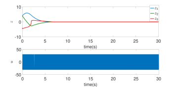
Figure 1: System (14) in close loop with (18).

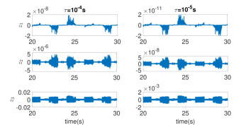
Figure 2: Accuracy of System (14) in close loop with (18) for $\displaystyle\tau=10^{-4}~{}s$ and $\displaystyle\tau=10^{-5}~{}s$.

Fig 1 shows the simulation results of system (14) with controller (18). We can see that the states $\displaystyle z_{1}$, $\displaystyle z_{2}$, $\displaystyle z_{3}$ converge in a finite time to the origin, and the control input $\displaystyle u$ is discontinuous.

The system homogeneity degree is $\displaystyle\kappa=-1/3$ and the homogeneity weights of $\displaystyle z_{1}$, $\displaystyle z_{2}$, $\displaystyle z_{3}$ are $\displaystyle 1$, $\displaystyle 2/3$, $\displaystyle 1/3$ respectively. These weights can be multiplied by 3 in order to achieve homogeneity weights $\displaystyle 3$, $\displaystyle 2$, $\displaystyle 1$ with the closed loop system homogeneity degree $\displaystyle\kappa=-1$. This homogeneity is called 3-sliding homogeneity [3]. According to these homogeneity weights, the controller (18) provides the following accuracy for the states w.r.t sampling step $\displaystyle\tau$

$$|z_{1}|\leq\lambda_{1}{\tau}^{3},\quad|z_{2}|\leq\lambda_{2}{\tau}^{2},\quad|z_{3}|\leq\lambda_{3}{\tau},$$ (19)

where $\displaystyle\lambda_{i}$ are constants. By simulations shown in Fig 2 with $\displaystyle{\tau}=10^{-4}s$, constants $\displaystyle\lambda_{i}$ are determined as $\displaystyle\lambda_{1}=20000$, $\displaystyle\lambda_{2}=500$, and $\displaystyle\lambda_{3}=200$. These constants have been confirmed by simulations with $\displaystyle{\tau}=10^{-5}s$ also shown in Fig 2.

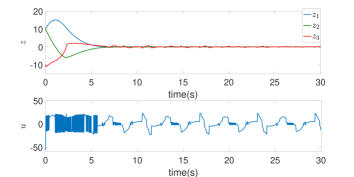
Figure 3: System (14) in close loop with (20).

3.2 Case when the bounds of uncertainties are unknown

In this case, the control parameters of $\displaystyle u_{0}$ are the same as in subsection 3.1, while the constant $\displaystyle k$ and the functions $\displaystyle g$ and $\displaystyle\hat{\varphi}$ in (12) are selected as $\displaystyle k=1$, $\displaystyle g=1$ and $\displaystyle\hat{\varphi}$ follows (7) where $\displaystyle\eta(t)=e^{-0.2t}$. Hence, $\displaystyle u$ can be written as

$$\begin{array}[]{lcl}u=-\Big{(}l_{3}+\hat{\varphi}(t,V(z)\big{)}\,\Big{)}\,\hbox{sgn}\Big{(}\psi_{3}(z_{1},z_{2},z_{3})\Big{)},\end{array}$$ (20)

with the Lyapunov Function candidate $\displaystyle V(z)$ is given by (see appendix A)

$$\displaystyle\begin{split}V(z)&=\frac{3}{5}{\left|{{z_{1}}}\right|^{\frac{5}{3}}}+\frac{2}{5}{\left|{{z_{2}}}\right|^{\frac{5}{2}}}+\frac{3}{5}l_{1}^{\frac{5}{2}}|{{z_{1}}}|^{\frac{5}{3}}+l_{1}^{\frac{3}{2}}{z_{2}}{\lfloor{{z_{1}}}\rceil}.+\frac{1}{5}{\left|{{z_{3}}}\right|^{5}}+\\ &\frac{4}{5}l_{2}^{5}{\left\lfloor{{{\left\lfloor{{z_{2}}}\right\rceil}^{\frac{3}{2}}}+l_{1}^{\frac{3}{2}}{{\left\lfloor{{z_{1}}}\right\rceil}}}\right\rceil^{\frac{5}{3}}}+{z_{3}}l_{2}^{4}\left\lfloor{{{{\left\lfloor{{z_{2}}}\right\rceil}^{\frac{3}{2}}}+l_{1}^{\frac{3}{2}}{{\left\lfloor{{z_{1}}}\right\rceil}}}}\right\rceil^{\frac{4}{3}}.\end{split}$$

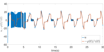
Figure 4: Evolution of the control signal and the uncertainties for System (14) with (20)

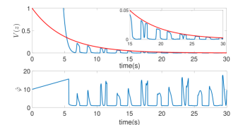
Figure 5: Evolution of the Lyapunov function $\displaystyle V(z)$ and the time varying function $\displaystyle\hat{\varphi}(t,V(z)\big{)}$ for System (14) with (20).

Figs 3-4-5 illustrate the simulation results of system (14) with the time varying controller (20). It can be noticed in Fig 3 that the proposed controller provides the practical stabilization for system (14), and the control input is not continuous in general. Moreover, it is confirmed in Fig 4 that the control signal is not overestimated. Indeed, after the time instant $\displaystyle\bar{t}(V(z_{0}))$ the control signal closely follows the uncertainties. On the other hand, the fulfillment of the control objective can be shown in Fig 5, where the sliding variable and its $\displaystyle r-1$ first derivatives enter in finite time in the family of time varying domains $\displaystyle D(t)$ defined in (6) and cannot exit it anymore for larger times. It can be seen also that the time varying function $\displaystyle\hat{\varphi}(t,V(z)\big{)}$ increases linearly until the time instant $\displaystyle\bar{t}(V(z_{0}))$ and then starts to follow the function $\displaystyle F_{\eta(t)}(x)$.

4 Conclusions

This paper has proposed a new Lyapunov-based time varying scheme for higher-order sliding mode controller applied for a class of perturbed chain of integrators with unknown bounded uncertainties. The proposed time varying controller guarantees $\displaystyle(a)$ the finite time convergence to a family of time varying open sets $\displaystyle(D(t))_{t\geq 0}$ decreasing to the origin as $\displaystyle t$ tends to infinity; $\displaystyle(b)$ once a trajectory enters some $\displaystyle D(t_{*})$ at time $\displaystyle t_{*}$, it remains trapped in the $\displaystyle D(t)$’s, i.e., $\displaystyle z(t)\in D(t)$ for $\displaystyle t\geq t_{*}$. Another advantage of this time varying controller consists in the fact that the decrease to the origin of the family $\displaystyle(D(t))_{t\geq 0}$ can be chosen arbitrarily.

References

Appendix A $\displaystyle u_{0}$ and the Lyapunov function $\displaystyle V$ design [34]

Firstly, the controller $\displaystyle u_{0}$ is determined explicitly.
Let the system homogeneity degree $\displaystyle\kappa=-\frac{1}{3}$. Then the homogeneity weights for the states $\displaystyle z_{1}$, $\displaystyle z_{2}$, $\displaystyle z_{3}$ are $\displaystyle 1$, $\displaystyle\frac{2}{3}$, $\displaystyle\frac{1}{3}$ respectively and the constants $\displaystyle\beta_{i}$ are $\displaystyle{\beta_{0}}=\frac{2}{3}$, $\displaystyle{\beta_{1}}=\frac{3}{2}$, $\displaystyle{\beta_{2}}=4$. According to [34], $\displaystyle u_{0}=v_{3}$ with

$$\displaystyle\left\{{\begin{array}[]{*{20}{c}}{{v_{0}}=0},\\ {\begin{array}[]{*{20}{c}}{{v_{i+1}}=-{l_{i+1}}{{\left\lfloor{{{\left\lfloor{{z_{i+1}}}\right\rceil}^{{\beta_{i}}}}-{{\left\lfloor{{v_{i}}}\right\rceil}^{{\beta_{i}}}}}\right\rceil}^{\frac{{{p_{\left({i+1}\right)}}+\kappa}}{{{p_{\left({i}\right)}}}}\times\frac{1}{{{\beta_{i}}}}}}},&{i=0,1,2.}\end{array}}\end{array}}\right.$$ (24)

From (24)

$$\displaystyle v_{1}=-{l_{1}}{\left\lfloor{{z_{1}}}\right\rceil^{\frac{{{p_{2}}}}{{{p_{1}}}}}}=-{l_{1}}{\left\lfloor{{z_{1}}}\right\rceil^{\frac{2}{3}}}.$$ (25)

Then

$$\displaystyle v_{2} \displaystyle=-{l_{2}}{\left\lfloor{{{\left\lfloor{{z_{2}}}\right\rceil}^{{\beta_{1}}}}-{{\left\lfloor{{v_{1}}}\right\rceil}^{{\beta_{1}}}}}\right\rceil^{\frac{{{p_{2}}+\kappa}}{{{p_{2}}}}\times\frac{1}{{{\beta_{1}}}}}}$$ (26)

$$\displaystyle=-{l_{2}}{\left\lfloor{{{\left\lfloor{{z_{2}}}\right\rceil}^{\frac{3}{2}}}+l_{1}^{\frac{3}{2}}{{\left\lfloor{{z_{1}}}\right\rceil}}}\right\rceil^{\frac{1}{3}}}.$$ (27)

Finally

$$\displaystyle{v_{3}} \displaystyle=-{l_{3}}{\left\lfloor{{{\left\lfloor{{z_{3}}}\right\rceil}^{{\beta_{2}}}}-{{\left\lfloor{{v_{2}}}\right\rceil}^{{\beta_{2}}}}}\right\rceil^{\frac{{{p_{3}}+\kappa}}{{{p_{3}}}}\times\frac{1}{{{\beta_{2}}}}}}$$ (28)

$$\displaystyle=-{l_{3}}{\left\lfloor{{{\left\lfloor{{z_{3}}}\right\rceil}^{4}}+{l_{2}}^{4}{\left\lfloor{{{\left\lfloor{{z_{2}}}\right\rceil}^{\frac{3}{2}}}+l_{1}^{\frac{3}{2}}{{\left\lfloor{{z_{1}}}\right\rceil}}}\right\rceil^{\frac{4}{3}}}}\right\rceil^{0}}$$ (29)

$$\displaystyle=-l_{3}sign\Big{(}\psi_{3}(z_{1},z_{2},z_{3})\Big{)}.$$ (30)

where $\displaystyle\psi_{3}(z_{1},z_{2},z_{3})={{{\left\lfloor{{z_{3}}}\right\rceil}^{4}}+{l_{2}}^{4}{\left\lfloor{{{\left\lfloor{{z_{2}}}\right\rceil}^{\frac{3}{2}}}+l_{1}^{\frac{3}{2}}{{\left\lfloor{{z_{1}}}\right\rceil}}}\right\rceil^{\frac{4}{3}}}}$. Therefore, the controller $\displaystyle u_{0}$ can be expressed as

$$\Rightarrow{u_{0}}=-{l_{3}}sign\Big{(}\psi_{3}(z_{1},z_{2},z_{3})\Big{)}$$

Now, the Lyapunov function $\displaystyle V$ is given. From [34], the Lyapunov function is defined in the following form

$$\displaystyle\left\{{\begin{array}[]{*{20}{c}}{V}_{i}=w_{i}+V_{i-1},\quad i=1,2,3\\ {\begin{array}[]{*{20}{c}}{w}_{i}=\int\limits_{{v_{i-1}}}^{{z_{i}}}{{{\left\lfloor s\right\rceil}^{{\beta_{i-1}}}}-{{\left\lfloor{{v_{i-1}}}\right\rceil}^{{\beta_{i-1}}}}ds}.\end{array}}\end{array}}\right.$$ (34)

In view of (34)

$${w_{1}}=\frac{1}{{1+{p_{2}}}}{\left|{{z_{1}}}\right|^{1+{r_{2}}}}=\frac{1}{{1+\frac{2}{3}}}{\left|{{z_{1}}}\right|^{1+\frac{2}{3}}},$$

which leads

$$\displaystyle V_{1}={w_{1}}=\frac{3}{5}{\left|{{z_{1}}}\right|^{\frac{5}{3}}}.$$ (35)

Then

$$\displaystyle\begin{split}{w_{2}}&=\int\limits_{{v_{1}}}^{{z_{2}}}{{{\lfloor s\rceil}^{{\beta_{1}}}}-{{\lfloor{{v_{1}}}\rceil}^{{\beta_{1}}}}}ds\\ &=\frac{1}{{{\beta_{1}}+1}}({{{|{{z_{2}}}|}^{{\beta_{1}}+1}}+{\beta_{1}}{{|{{v_{1}}}|}^{{\beta_{1}}+1}}})-{z_{2}}{\lfloor{{v_{1}}}\rceil^{{\beta_{1}}}}\\ &=\frac{1}{{\frac{3}{2}+1}}({{{|{{z_{2}}}|}^{\frac{3}{2}+1}}+\frac{3}{2}{{\lfloor{{v_{1}}}\rceil}^{\frac{3}{2}+1}}})-{z_{2}}{\lfloor{{v_{1}}}\rceil^{\frac{3}{2}}},\end{split}$$ (36)

with $\displaystyle{v_{1}}=-{l_{1}}{\left\lfloor{{z_{1}}}\right\rceil^{\frac{2}{3}}}$, it implies that

$$\displaystyle{w_{2}}=\frac{2}{5}{\left|{{z_{2}}}\right|^{\frac{5}{2}}}+\frac{3}{5}l_{1}^{\frac{5}{2}}|{{z_{1}}}|^{\frac{5}{3}}+l_{1}^{\frac{3}{2}}{z_{2}}{\lfloor{{z_{1}}}\rceil}.$$ (37)

Therefore,

$$\displaystyle\begin{split}{V_{2}}&={V_{1}}+w_{2}\\ &=\frac{3}{5}{\left|{{z_{1}}}\right|^{\frac{5}{3}}}+\frac{2}{5}{\left|{{z_{2}}}\right|^{\frac{5}{2}}}+\frac{3}{5}l_{1}^{\frac{5}{2}}|{{z_{1}}}|^{\frac{5}{3}}+l_{1}^{\frac{3}{2}}{z_{2}}{\lfloor{{z_{1}}}\rceil}.\end{split}$$ (38)

Finally,

$$\displaystyle\begin{split}{w_{3}}&=\int\limits_{{v_{2}}}^{{z_{3}}}{{{\lfloor s\rceil}^{{\beta_{2}}}}-{{\lfloor{{v_{2}}}\rceil}^{{\beta_{2}}}}}ds\\ &=\frac{1}{{{\beta_{2}}+1}}({{{|{{z_{3}}}|}^{{\beta_{2}}+1}}+{\beta_{2}}{{|{{v_{2}}}|}^{{\beta_{2}}+1}}})-{z_{3}}{\lfloor{{v_{2}}}\rceil^{{\beta_{2}}}},\end{split}$$ (39)

with $\displaystyle{\beta_{2}}=4$; $\displaystyle{v_{2}}=-{l_{2}}{\left\lfloor{{{\left\lfloor{{z_{2}}}\right\rceil}^{\frac{3}{2}}}+l_{1}^{\frac{3}{2}}{{\left\lfloor{{z_{1}}}\right\rceil}}}\right\rceil^{\frac{1}{3}}}$, it leads

$$\displaystyle\begin{split}{w_{3}}&=\frac{1}{5}\left({{{\left|{{z_{3}}}\right|}^{5}}+4l_{2}^{5}{\left\lfloor{{{\left\lfloor{{z_{2}}}\right\rceil}^{\frac{3}{2}}}+l_{1}^{\frac{3}{2}}{{\left\lfloor{{z_{1}}}\right\rceil}}}\right\rceil^{\frac{5}{3}}}}\right)\\ &+{z_{3}}l_{2}^{4}\left\lfloor{{{{\left\lfloor{{z_{2}}}\right\rceil}^{\frac{3}{2}}}+l_{1}^{\frac{3}{2}}{{\left\lfloor{{z_{1}}}\right\rceil}}}}\right\rceil^{\frac{4}{3}}\\ &=\frac{1}{5}{\left|{{z_{3}}}\right|^{5}}+\frac{4}{5}l_{2}^{5}{\left\lfloor{{{\left\lfloor{{z_{2}}}\right\rceil}^{\frac{3}{2}}}+l_{1}^{\frac{3}{2}}{{\left\lfloor{{z_{1}}}\right\rceil}}}\right\rceil^{\frac{5}{3}}}\\ &+{z_{3}}l_{2}^{4}\left\lfloor{{{{\left\lfloor{{z_{2}}}\right\rceil}^{\frac{3}{2}}}+l_{1}^{\frac{3}{2}}{{\left\lfloor{{z_{1}}}\right\rceil}}}}\right\rceil^{\frac{4}{3}}.\end{split}$$ (40)

Thus, the Lyapunov function $\displaystyle V$ is given by

$$\displaystyle\begin{split}V={V_{3}}&=\frac{3}{5}{\left|{{z_{1}}}\right|^{\frac{5}{3}}}+\frac{2}{5}{\left|{{z_{2}}}\right|^{\frac{5}{2}}}+\frac{3}{5}l_{1}^{\frac{5}{2}}|{{z_{1}}}|^{\frac{5}{3}}+l_{1}^{\frac{3}{2}}{z_{2}}{\lfloor{{z_{1}}}\rceil}+\frac{1}{5}{\left|{{z_{3}}}\right|^{5}}+\\ &\frac{4}{5}l_{2}^{5}{\left\lfloor{{{\left\lfloor{{z_{2}}}\right\rceil}^{\frac{3}{2}}}+l_{1}^{\frac{3}{2}}{{\left\lfloor{{z_{1}}}\right\rceil}}}\right\rceil^{\frac{5}{3}}}+{z_{3}}l_{2}^{4}\left\lfloor{{{{\left\lfloor{{z_{2}}}\right\rceil}^{\frac{3}{2}}}+l_{1}^{\frac{3}{2}}{{\left\lfloor{{z_{1}}}\right\rceil}}}}\right\rceil^{\frac{4}{3}}.\end{split}$$ (41)

References

• [1] A. Levant, Universal Single-Inupte Single-Output (SISO) Sliding-Mode Controllers With Finite-Time Convergence, IEEE Transactions on Automatic Control 46 (9) (2001) 1447 – 1451.
• [2] A. Levant, Higher-order sliding modes, differentiation and output-feedback control, International Journal of Control 76 (9/10) (2003) 924 – 941.
• [3] A. Levant, Homogeneity approach to high-order sliding mode design, Automatica 41 (5) (2005) 823 – 830.
• [4] S. Ding, A. Levant, S. Li, Simple homogeneous sliding-mode controller, Automatica 67 (2016) 22 – 32.
• [5] E. Cruz-Zavala, J. A. Moreno, Homogeneous High Order Sliding Mode design: A Lyapunov approach, Automatica 80 (2017) 232 – 238.
• [6] M. V. Basin, C. B. Panathula, Y. B. Shtessel, P. C. R. Ram rez, Continuous finite-time higher order output regulators for systems with unmatched unbounded disturbances, IEEE Transactions on Industrial Electronics 63 (8) (2016) 5036–5043.
• [7] A. Levant, L. M. Fridman, Accuracy of Homogeneous Sliding Modes in the Presence of Fast Actuators, IEEE Transactions on Automatic Control 55 (3) (2010) 810–814.
• [8] F. Plestan, Y. Shtessel, V. Bregeault, A. Poznyak, New methodologies for adaptive sliding mode control, International Journal of Control 83 (2010) 1907 – 1919.
• [9] G. Bartolini, A. Levant, F. Plestan, M. Taleb, E. Punta, Adaptation of sliding modes, IMA Journal of Mathematical Control and Information 30 (2013) 885–300.
• [10] J. Moreno, D. Negrete, V. Torres-González, L. Fridman, Adaptive continuous twisting algorithm, International Journal of Control 89 (9) (2016) 1798–1806.
• [11] C. Edwards, Y. Shtessel, Adaptive dual layer super-twisting control and observation, International Journal of Control 89 (9) (2016) 1759–1766.
• [12] C. Edwards, Y. B. Shtessel, Adaptive continuous higher order sliding mode control, Automatica 65 (2016) 183 – 190.
• [13] T. R. Oliveira, J. P. V. S. Cunha, L. Hsu, Adaptive Sliding Mode Control Based on the Extended Equivalent Control Concept for Disturbances with Unknown Bounds, Springer International Publishing, 2018, pp. 149–163.
• [14] L. Hsu, T. R. Oliveira, G. T. Melo, J. P. V. S. Cunha, Adaptive Sliding Mode Control Using Monitoring Functions, Springer International Publishing, 2018, pp. 269–285.
• [15] D. Y. Negrete-Chávez, J. A. Moreno, Second-order sliding mode output feedback controller with adaptation, International Journal of Adaptive Control and Signal Processing 30 (8–10) (2016) 1523–1543.
• [16] Y. Shtessel, M. Taleb, F. Plestan, A novel adaptive-gain super-twisting sliding mode controller: methodology and application, Automatica 48 (5) (2012) .759–769.
• [17] Y. B. Shtessel, J. A. Moreno, L. M. Fridman, Twisting sliding mode control with adaptation: Lyapunov design, methodology and application, Automatica 75 (2017) 229 – 235.
• [18] H. Obeid, L. M. Fridman, S. Laghrouche, M. Harmouche, Barrier function-based adaptive sliding mode control, Automatica 93 (2018) 540 – 544.
• [19] L. Hsu, T. R. Oliveira, J. S. Cunha, L. Yan, Adaptive unit vector control of multivariable systems using monitoring functions, International Journal of Robust and Nonlinear Control 29 (3) (2019) 583–600.
• [20] A. Ferrara, G. Incremona, E. Regolin, Optimization-based adaptive sliding mode control with application to vehicle dynamics control, International Journal of Robust and Nonlinear Control 29 (3) (2019) 550–564.
• [21] M. Basin, C. Panathula, Y. Shtessel, Adaptive uniform finite-/fixed-time convergent second-order sliding-mode control, International Journal of Control 89 (9) (2016) 1777–1787.
• [22] A. Ferreira, F. J. Bejarano, L. Fridman, Robust control with exact uncertainties compensation: With or without chattering?, Control Systems Technology, IEEE Transactions on 19 (5) (2011) 969–975.
• [23] V. I. Utkin, A. S. Poznyak, Adaptive sliding mode control with application to super-twist algorithm: Equivalent control method, Automatica 49 (1) (2013) 39–47.
• [24] Y. Huang, T. Kuo, S. Chang, Adaptive sliding-mode control for nonlinear systems with uncertain parameters, IEEE Transactions on Automatic Control 38 (2008) 534–539.
• [25] F. Plestan, Y. Shtessel, V. Bregeault, A. Poznyak, Sliding mode control with gain adaptation-application to an electropneumatic actuator, Control Engineering Practice 21 (5) (2013) 679 – 688.
• [26] H. Obeid, S. Laghrouche, L. M. Fridman, Y. Chitour, M. Harmouche, Barrier function-based variable gain super-twisting controller, IEEE Transactions on Automatic Control, To appear.
• [27] H. Obeid, L. Fridman, S. Laghrouche, M. Harmouche, M. A. Golkani, Adaptation of levant’s differentiator based on barrier function, International Journal of Control 91 (9) (2018) 2019–2027.
• [28] H. Obeid, L. Fridman, S. Laghrouche, M. Harmouche, Barrier function-based adaptive twisting controller, in: 2018 15th International Workshop on Variable Structure Systems (VSS), 2018, pp. 198–202.
• [29] H. Obeid, L. Fridman, S. Laghrouche, M. Harmouche, Barrier function-based adaptive integral sliding mode control, in: 2018 IEEE Conference on Decision and Control (CDC), 2018, pp. 5946–5950.
• [30] H. Obeid, S. Laghrouche, L. M. Fridman, M. Harmouche, Dual layer based-adaptive discontinuous higher order sliding mode control, Under Review.
• [31] A. Filippov, Differential Equations with Discontinuous Right-Hand Side, Kluwer, Dordrecht, The Netherlands, 1988.
• [32] A. Levant, Finite-Time Stability and High Relative Degrees in Sliding-Mode Control, Lecture Notes in Control and Information Sciences 412 (2001) 59 – 92.
• [33] M. Harmouche, S. Laghrouche, Y. Chitour, Robust and adaptive higher order sliding mode controllers, in: Decision and Control (CDC), 2012 IEEE 51st Annual Conference on, 2012, pp. 6436–6441.
• [34] Y. Hong, Finite-time stabilization and stabilizability of a class of controllable systems, Systems and Control Letters 46 (4) (2002) 231–236.
• [35] X. Huang, W. Lin, B. Yang, Global finite-time stabilization of a class of uncertain nonlinear systems, Automatica 41 (2005) 881–888.
• [36] E. Cruz-Zavala, J. A. Moreno, A new class of fast finite-time discontinuous controllers, in: 2014 13th International Workshop on Variable Structure Systems (VSS), 2014, pp. 1–6.
• [37] S. Laghrouche, M. Harmouche, Y. Chitour, Higher order super-twisting for perturbed chains of integrators, IEEE TAC 62 (7) (2017) 3588–3593.
• [38] M. Harmouche, S. Laghrouche, Y. Chitour, M. Hamerlain, Stabilisation of perturbed chains of integrators using Lyapunov-based homogeneous controllers, International Journal of Control 90 (12) (2017) 2631–2640.