Quark-diquark string tension, excited baryonic resonances and thermal fluctuations

Abstract

We study the baryonic fluctuations from second to eighth order involving electric charge, baryon number and strangeness below the quark-gluon plasma crossover and numerically known from lattice QCD calculations. By considering a particular realization of the Hadron Resonance Gas model, we provide evidence on the dominant role of quark-diquark degrees of freedom to describe excited baryonic resonances. After proving by means of suitable Polyakov loop correlators that the quark-diquark and the quark-antiquark forces coincide, $V_{\bar{q}q}(r)=V_{\bar{q}D}(r)+\textrm{const}$, we find that the corresponding susceptibilities can be saturated with excited baryonic states in a quark-diquark model picture.

Keywords: string tension, finite temperature QCD, fluctuations, quark models, diquarks

1 Introduction

The experimental program on relativistic heavy ion collisions is currently ongoing at LHC within the ALICE experiment [1], and at RHIC in the so called beam-energy scan (BES) program and further upgraded stages [2]. In these experiments they study various regions of the $T-\mu_{B}$ phase diagram by changing the collision energy. There are also several future experiments at FAIR [3] and NICA [4] that will contribute as well to the study of the Quantum Chromodynamics (QCD) phase diagram with finite chemical potential.

Apart from lattice calculations [5, 6], there are also further approaches to study QCD at finite temperature and chemical potential, and in particular fluctuations of conserved charges. Among them, we could mention the chiral quark models coupled to the Polyakov loop, as e.g. the Polyakov-loop Nambu–Jona-Lasinio (PNJL) model [7], and the Polyakov-loop quark meson model [8], as well as the Dyson-Schwinger approaches [9]. Another interesting approach is the the Hadron Resonance Gas (HRG) model that allows to describe the confined phase of the QCD equation of state (EoS) at finite temperature below $\sim 150\,{\rm MeV}$ as a multicomponent gas of non-interacting massive stable and point-like particles [10, 11], which are usually taken as the conventional hadrons listed in the review by the Particle Data Group (PDG) [12]. A clear advantage of the HRG approach is that it incorporates, by construction, the relevant degrees of freedom that allow to describe the low temperature regime of QCD. The other approaches cannot describe such regime so accurately, and they usually focus on the description of the high temperature and the phase transition regimes. These regions in the phase diagram of QCD, however, cannot be described within the HRG approach. In this sense, some authors have proposed some hybrid models that incorporate the advantages of different approaches in a single picture, as e.g. the HRG-PNJL hybrid model [13]. Let us point out that all these works try to describe lattice data.

One of the greatest achievements of the HRG approach has been the study of the trace anomaly, $(\epsilon-3P)/T^{4}$ with $\epsilon$ energy density and $P$ the pressure. It was computed directly in lattice QCD by several collaborations [14, 15] and within the HRG approach, leading to an excellent agreement for temperatures below $T\sim 170\,{\rm MeV}$ (see e.g. Ref. [16] and references therein). Thus, this approach has emerged as a practical and viable path to establish completeness of hadronic states in the hadronic phase [17, 18, 19]. Apart from the EoS, other thermal observables like the fluctuations of conserved charges [6] can be used to study the QCD spectrum by distinguishing between different flavor sectors. Another motivation to study the fluctuations is that they are among the most relevant observables for finite density studies, as one possible way to extend lattice results to finite density is to perform Taylor expansions of the thermodynamical quantities around zero chemical potential [20]. These quantities can directly be compared to experimental measurements of fluctuations in relativistic heavy ion collisions, and may provide insight into the existence of a critical end point in the QCD phase diagram [21, 22].

There are a number of quark models that try to reproduce the PDG hadron spectrum, one of the most fruitful being the Relativized Quark Model (RQM) for mesons [23] and baryons [24]. This model shows that there are further states in the spectrum above some scale as compared to the PDG. On the other hand, the suspicion that the baryonic spectrum can be understood in terms of quark-diquark degrees of freedom [25] is rather old, and this includes diquark clustering studies [26] as well as non relativistic and relativistic analyses [27, 28, 29, 30, 31, 32, 33]. Lattice QCD has also provided some evidence on diquarks correlations in the nucleon [34]. In the present work we provide further evidence for the existence of the quark-diquark baryonic states, and study the possibility that these states saturate the baryonic fluctuations in the confined phase as compared to the available lattice QCD calculations.

Finally, let us summarize the wider context of the research that we will pursue in this work. The phase transition from hadronic matter to a quark gluon plasma has been a major topic as it seems to be a distinct feature of QCD which may be produced copiously in ultrarelativistic heavy ion colliders and can be simulated by lattice QCD. The thermal behaviour of the system is characterized by the equation of state which even in the conventional hadronic phase may provide valuable information on the hadronic spectrum. More specific information probing particular quantum numbers can be pinned down by analyzing fluctuations of conserved charges. In this work we analyze the baryonic spectrum in terms of baryonic susceptibilities and find by comparison with lattice QCD calculations, PDG listings and quark models that most of the baryonic spectrum befits a quark-diquark picture.

2 Hadron spectrum

The cumulative number of states is very useful for the characterization of the QCD spectrum. It is defined as the number of bound states below some mass $M$, i.e.

$$N(M)=\sum_{i}g_{i}\,\Theta(M-M_{i})\,,$$ (1)

where $M_{i}$ is the mass of the $i$-th hadron, $g_{i}$ is the degeneracy, and $\Theta(x)$ is the step function, so that the density of states writes $\rho(M)=dN(M)/dM$. So far, the states listed in the PDG echo the standard quark model classification for mesons $[q{\bar{q}}]$ and baryons $[qqq]$, and the cumulative number will have contributions from any kind of states, i.e.

$$N(M)=M_{[q\bar{q}]}(M)+N_{[qqq]}(M)+N_{[q\bar{q}q\bar{q}]}(M)+\cdots\,.$$ (2)

Then, it would be pertinent to consider also the spectrum of the RQM for hadrons, as it corresponds by construction to a solution of the quantum mechanical problem for both $q\bar{q}$-mesons and $qqq$-baryons. For color-singlet states, the $n$-parton Hamiltonian takes the form

$$H_{n}=\sum_{i=1}^{n}\sqrt{{\mathbf{p}}_{i}^{2}+m_{i}^{2}}+\sum_{i<j}^{n}v_{ij}({\mathbf{r}}_{ij})\,,$$ (3)

where the two-body interactions take the form $v_{q\bar{q}}(r)=-4\alpha_{S}/(3r)+\sigma r=(N_{c}-1)v_{qq}(r)$. This Hamiltonian for $n=2(3)$ describes the underlying dynamics of mesons(baryons). We show in Fig. 1 the hadron spectrum with the PDG compilation (left) and the RQM spectrum (right). The comparison clearly shows that there are further states in the RQM spectrum above some scale $M>M_{\min}$ that may or may not be confirmed in the future as mesons or hadrons, although they could also be exotic, glueballs or hybrids.

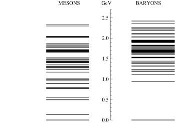
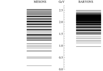
Figure 1: Mesons and baryons spectrum made of $u$, $d$ and $s$ quarks from the PDG [12] (left panel) and from the relativized quark model [23, 24] (right panel).

A semiclassical expansion of the cumulative number of states [35] can be used to study the high mass spectrum for systems where interactions are dominated by linearly rising potentials with a string tension $\sigma$, in the range $M\gg\sqrt{\sigma}$. At leading order in the expansion, the cumulative number takes the form

$$N_{n}(M)\sim g_{n}\int\prod_{i=1}^{n}\frac{d^{3}x_{i}d^{3}p_{i}}{(2\pi)^{3}}\delta\left({\textstyle\sum_{i=1}^{n}{\mathbf{x}}_{i}}\right)\delta\left({\textstyle\sum_{i=1}^{n}{\mathbf{p}}_{i}}\right)\Theta(M-H_{n}(p,x))\sim\left(\frac{M^{2}}{\sigma}\right)^{3n-3}$$ (4)

where in the last estimate we have neglected the (color) Coulomb term of the potential. Then, one can predict that the large mass expansion of these contributions is

$$N_{[q{\bar{q}}]}\sim M^{6}\,,\quad N_{[qqq]}\sim M^{12}\,,\quad N_{[q{\bar{q}}q{\bar{q}}]}\sim M^{18}\,,\,\cdots\,.$$ (5)

This means that each kind of hadron dominates the function $N(M)$ at a different scale. We display in Fig. 2 the separate contributions of meson and baryon spectra for the PDG and RQM. Note that while in the meson case the $N_{[q{\bar{q}}]}\sim M^{6}$ behavior seems to conform with the asymptotic estimate, in the baryon case much lower exponents, $M^{6}-M^{8}$, than the expected one are identified. $M^{6}$ suggests a two-body dynamics, and we take this feature as a hint that the $qqq$ excited spectrum effectively conforms to a two body system of particles interacting with a linearly growing potential. The consequences of this picture will be analyzed in Sec. 3.

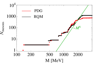
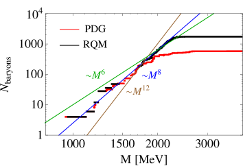
Figure 2: Cumulative numbers for the PDG (lower curve) and the RQM (upper curve). We display in log-log scale the mesonic states (left panel), and the baryonic states (right panel).

Finally, let us mention that after adding all the contributions $N_{\lambda}(M)\sim M^{q_{\lambda}}$, one obtains the conjectured behavior of the Hagedorn spectrum [36]

$$N_{{\textrm{\tiny HRG}}}(M)\sim e^{M/T_{H}}\,.$$ (6)

This exponential behavior would lead to a partition function that becomes divergent at some finite value of the temperature, i.e.

$$Z_{{\textrm{\tiny HRG}}}=\Tr\,e^{-H_{{\textrm{\tiny HRG}}}/T}\stackrel{{\scriptstyle[}}{{T}}\to T_{H}^{-}]{\longrightarrow}{}\frac{A}{T_{H}-T}\,,$$ (7)

where $T_{H}\approx 150\,{\rm MeV}$ is the so-called Hagedorn temperature. The computation of the trace anomaly with the HRG model leads to a good description of the lattice data for $T\lesssim 0.8\,T_{c}$ by using either the PDG or the RQM spectrum, see e.g. Ref. [37].

3 Quark-diquark model for baryons

In the quark model, such as the RQM [24], baryons are $[qqq]$ states where the interaction is given by a combination of $\Delta$-like pairs of $qq$ interactions and a genuinely $Y$-like $qqq$ interaction. An interesting possibility would be that the quarks are distributed according to an isosceles triangle, leading to an easily tractable class of models, the so-called quark-diquark ($qD$) models [28, 31, 33, 38, 39]. In these models, the baryons are assumed to be composed of a constituent quark $q$, and a constituent diquark $D\equiv(qq)$, i.e. $B\equiv[q(qq)]$. In its relativistic version the Hamiltonian writes

$$H_{qD}=\sqrt{{\mathbf{p}}^{2}+m_{q}^{2}}+\sqrt{{\mathbf{p}}^{2}+m_{D}^{2}}+V_{qD}(r)\,,$$ (8)

corresponding to a two body problem. The aim of this section is to obtain the baryon spectrum within a simple realization of the $qD$ model. But before going to the phenomenological consequences of the model, we will show analytically that under very specific assumptions the $qD$ static interaction for heavy sources, $V_{qD}(r)$, coincides with the quark-antiquark potential, $V_{q\bar{q}}(r)$, up to an additive constant.

3.1 Quark-diquark potential

An operational way of placing static sources in a gauge theory is by introducing in the Euclidean formulation a local gauge rotation realized by the Polyakov loop, i.e.

$$\Omega({\mathbf{x}})={\mathcal{P}}\,e^{\,i\int_{0}^{\beta}A_{0}(x)\,dx_{0}}\,,$$ (9)

where ${\mathcal{P}}$ indicates path ordering. The $q\bar{q}$ free energy is given by the thermal expectation value (our color trace is not normalized, i.e. $\tr 1=N_{c}$) [40]

$$e^{-F_{q\bar{q}}(r,T)/T}=\langle\tr\Omega({\mathbf{x}}_{1})\tr\Omega({\mathbf{x}}_{2})^{\dagger}\rangle_{T}\,,$$ (10)

and the potential is obtained as the zero temperature limit of the free energy, i.e. $V_{q\bar{q}}(r)=F_{q\bar{q}}(r,0)$. For baryons it is more relevant to study the $qqq$ free energy, which is given by

$$e^{-F_{qqq}({\mathbf{x}}_{1},{\mathbf{x}}_{2},{\mathbf{x}}_{3},T)/T}=\langle\tr\Omega({\mathbf{x}}_{1})\tr\Omega({\mathbf{x}}_{2})\tr\Omega({\mathbf{x}}_{3})\rangle_{T}\,.$$ (11)

One can take in this expression the limit ${\mathbf{x}}_{3}\to{\mathbf{x}}_{2}$ to get the following result for the quark-diquark free energy

$$e^{-F_{qD}({\mathbf{x}}_{1},{\mathbf{x}}_{2},T)/T}=\langle\tr\Omega({\mathbf{x}}_{1})\tr(\Omega({\mathbf{x}}_{2})^{2})\rangle_{T}\,.$$ (12)

Note that this limit is singular since at very small distances the interaction is dominated by one gluon exchange, $\sim 1/r$, and a self-energy must be added. The renormalization of the composite operator $\tr(\Omega({\mathbf{x}}_{2})^{2})$ yields an ambiguity in the form of an additive constant from $F_{qqq}({\mathbf{x}}_{1},{\mathbf{x}}_{2},{\mathbf{x}}_{2},T)$ to $F_{qD}({\mathbf{x}}_{1},{\mathbf{x}}_{2},T)$. Finally, by using the Clebsch-Gordan decomposition, ${\bf 3}\otimes{\bf 3}\otimes{\bf 3}=({\bf 3}\otimes{\bf\bar{3}})\oplus({\bf 3}\otimes{\bf 6})$, one finds that

$$e^{-F_{qD}({\mathbf{x}}_{1},{\mathbf{x}}_{2},T)/T}\equiv e^{-F_{q\bar{q}}({\mathbf{x}}_{1},{\mathbf{x}}_{2},T)/T}+e^{-F_{3\otimes 6}({\mathbf{x}}_{1},{\mathbf{x}}_{2},T)/T}\simeq e^{-F_{q\bar{q}}({\mathbf{x}}_{1},{\mathbf{x}}_{2},T)/T}\,.$$ (13)

In the last equality we have considered that the energy ${\bf 3}\otimes{\bf 6}$ configuration is larger than that of the $q\bar{q}$ one. Hence, after taking the zero temperature limit, we find

$$V_{qD}(r)=V_{q\bar{q}}(r)+\textrm{const}\,,$$ (14)

a property which is in marked agreement with recent lattice studies [41] (see also Refs. [42, 43]), and that will be used in the following.

3.2 The model

Based on the considerations above, we can assume for the $qD$ potential [44]

$$V_{qD}(r)=-\frac{\tau}{r}+\sigma r+\mu\,,$$ (15)

with $\tau=\pi/12$ and $\sigma=(0.42\,{\rm GeV})^{2}$. The parameters of the kinetic terms in the Hamiltonian of Eq. (8) are controlled by: i) the constituent quark mass, $m_{\textrm{\scriptsize cons}}$, and ii) the current quark mass for the strange quark, $\hat{m}_{s}$; in the following way

$$m_{u,d}=m_{\textrm{\scriptsize cons}}\,,\qquad m_{s}=m_{\textrm{\scriptsize cons}}+\hat{m}_{s}\,.$$ (16)

In addition, we can distinguish between two kinds of diquarks: scalar $D\equiv[q_{1}q_{2}]$, and axial vector $D_{AV}\equiv\{q_{1}q_{2}\}$; so that in the following we will consider the natural choice

$$m_{D,{\textrm{\scriptsize ns}}}=2m_{{\textrm{\scriptsize cons}}}\,,\qquad m_{D_{AV},{\textrm{\scriptsize ns}}}=m_{D,{\textrm{\scriptsize ns}}}+\Delta m_{D}\,,$$ (17)

where the subindex ns refers to diquarks with non-strange quarks. Some studies in QCD indicate a mass difference between these diquarks of $\Delta m_{D}\simeq 0.21\,{\rm GeV}$ [45], a value that will be adopted in the following. On the other hand, the breaking of flavor ${\textrm{SU}}(3)$ for diquarks will be modeled as

$$m_{X}=m_{X,{\textrm{\scriptsize ns}}}+n_{s}\hat{m}_{s}\,,\qquad X=D,D_{AV}\,,$$ (18)

where $n_{s}$ is the number of $s$ quarks in the diquark. Under these assumptions, the only parameters of the model that remain free are $m_{\textrm{\scriptsize cons}}$, $\hat{m}_{s}$ and $\mu$. We summarize in Table 1 the degeneracies of the states predicted by the model, by distinguishing between their electric charges. The quantum numbers of these states are $Q$, $B=1$ and $S=-n_{s}$.

Table 1: Spin-isospin degeneracies of the baryonic states within the quark-diquark model. $n$ represents the light flavors $u$ and $d$, while $s$ is the strange quark.

Baryon	Total deg.	$Q=-1$	$Q=0$	$Q=1$	$Q=2$
$[nn]n$	4	-	2	2	-
$\{nn\}n$	36	6	12	12	6
$[nn]s$	2	-	2	-	-
$\{nn\}s$	18	6	6	6	-
$[ns]n$	8	2	4	2	-
$\{ns\}n$	24	6	12	6	-
$[ns]s$	4	2	2	-	-
$\{ns\}s$	12	6	6	-	-
$\{ss\}n$	12	6	6	-	-
$\{ss\}s$	6	6	-	-	-

3.3 Baryon spectrum

The baryon spectrum of the $qD$ model can be obtained by diagonalizing the Hamiltonian of Eq. (8). We will consider a variational procedure by using as basis the 3-dimensional isotropic harmonic oscillator (IHO), with normalized wave functions of the form

$$R_{n\ell}(r)=\sqrt{\frac{(n-1)!\,2^{\ell+n+1}}{\sqrt{\pi}b^{3}(2\ell+2(n-1)+1)!!}}L_{n-1}^{\ell+\frac{1}{2}}(r^{2}/b^{2})\left(\frac{r}{b}\right)^{\ell}e^{-\frac{r^{2}}{2b^{2}}}\,,$$ (19)

where $L_{n-1}^{\ell+\frac{1}{2}}(x)$ are the generalized Laguerre polynomials. The matrix elements of the Hamiltonian are then obtained from

$$\langle n\ell|H_{qD}|n^{\prime}\ell\rangle = \int_{0}^{\infty}dp\,\hat{u}_{n\ell}^{\ast}(p)\hat{u}_{n^{\prime}\ell}(p)\left[\sqrt{p^{2}+m_{q}^{2}}+\sqrt{p^{2}+m_{D}^{2}}\right]$$ (20)

$$+\int_{0}^{\infty}dr\,u_{n\ell}^{\ast}(r)u_{n^{\prime}\ell}(r)V_{qD}(r)\,,$$

with $u_{n\ell}(r)$ and $\hat{u}_{n\ell}(p)$ the reduced wave functions of the IHO in position and momentum space, respectively. The value of the parameter $b$ is fixed to minimize the energy levels for each of the multiplets in Table 1, being the typical values of this parameter in the range $0.55\,{\rm fm}\lesssim b\lesssim 0.65\,{\rm fm}$. We get with this procedure the spectrum of baryons that is shown in Fig. 3. We have considered as a convenient choice of the parameters of the model, the values

$$m_{D,{\textrm{\scriptsize ns}}}=0.6\,{\rm GeV}\,,\quad m_{u,d}=0.3\,{\rm GeV}\,,\quad\hat{m}_{s}=0.10\,{\rm GeV}\,,\quad\mu=-0.459\,{\rm GeV}\,.$$ (21)

These values are motivated by the fits of the lattice data for the baryonic susceptibilities that will be presented in Sec. 4.3. It is remarkable that below $M<2400\,{\rm MeV}$ the quark-diquark spectrum is in good agreement with the RQM spectrum. Note that the growth of the cumulative number is $N_{[qD]}\sim M^{6}$, as expected for a two body problem. Since the quark-diquark picture is reliable only for excited states, in the following we will use the empirical value of the mass of the nucleon, $M_{n}=938\,{\rm MeV}$, and apply the $qD$ model only for the other baryons.

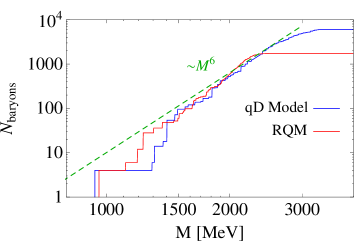
Figure 3: Cumulative number for the baryon spectrum as a function of the baryon mass. We compare the $qD$ model of Sec. 3, and the RQM [24].

4 Fluctuations of conserved charges and baryonic susceptibilities

The EoS of QCD is sensitive to both mesonic and baryonic states, and the thermodynamic separation of these degrees of freedom cannot be done at the QCD level. However, there is a number of thermal observables that can be used to study the spectrum of QCD by distinguishing between different flavor sectors; these are the fluctuations [6] and correlations [46] of conserved charges. Beyond these hadron spectrum considerations, recent lattice studies of fluctuations suggest that they are sensitive probes of deconfinement in realistic physical situations in which quarks cannot be considered as heavy sources (see e.g. Ref. [21] for a recent review). We will study in this section the baryonic susceptibilities within the HRG approach by using the $qD$ spectrum obtained in Sec. 3. A comparison with the lattice data for the fluctuations will allow to extract information about the values of the parameters of the model.

4.1 Fluctuations of conserved charges

Conserved charges $[Q_{a},H]=0$ play a fundamental role in the thermodynamics of QCD. When considering the $(uds)$ flavor sector of QCD, the only conserved charges are the electric charge $Q$, the baryon number $B$, and the strangeness $S$. Their thermal expectation values present statistical fluctuations, that are usually computed from the grand-canonical partition function [20]

$$Z_{{\textrm{\tiny QCD}}}=\textrm{Tr}\exp\bigg{[}-\Big{(}H_{{\textrm{\tiny QCD}}}-\sum_{a}\mu_{a}Q_{a}\Big{)}/T\bigg{]}\,.$$ (22)

By considering the differentiation of the thermodynamical potential $\Omega=-T\log Z_{{\textrm{\tiny QCD}}}$ with respect to the chemical potential, one finds the thermal expectation values and the susceptibilities of the charges

$$\langle Q_{a}\rangle_{T}=-\frac{\partial\Omega}{\partial\mu_{a}}\Bigg{|}_{\mu_{a}=0}\,,\quad\chi_{ab}(T)\equiv\frac{1}{VT^{3}}\langle\Delta Q_{a}\Delta Q_{b}\rangle_{T}=-\frac{1}{VT^{2}}\frac{\partial^{2}\Omega}{\partial\mu_{a}\partial\mu_{b}}\Bigg{|}_{\mu_{a}=0=\mu_{b}}\,,$$ (23)

where $\Delta Q_{a}=Q_{a}-\langle Q_{a}\rangle_{T}$, and $Q_{a}\in\{Q,B,S\}$. We have used that $\langle Q_{a}\rangle_{T}=0$ in absence of chemical potentials. Note that the fluctuations can also be computed in the quark-flavor basis, $Q_{a}\in\{u,d,s\}$, where $u$, $d$ and $s$ is the number of up, down and strange quarks. In this basis

$$B=\frac{1}{3}(u+d+s)\,,\quad Q=\frac{1}{3}(2u-d-s)\,,\quad S=-s\,.$$ (24)

4.2 Fluctuations within the HRG approach

While in the deconfined phase of QCD the quarks and gluons are liberated to form a plasma, in the confined/chiral symmetry broken phase the relevant degrees of freedom are bound states of quarks and gluons, i.e. hadrons and possibly exotic states. This means that it should be expected that physical quantities in this phase admit a representation in terms of hadronic states. This is the idea of the hadron resonance gas (HRG) model which describes the equation of state of QCD in terms of a free gas of hadrons [11, 47, 48],

$$\log Z_{{\textrm{\tiny HRG}}}=-V\int\frac{d^{3}p}{(2\pi)^{3}}\sum_{i\in{\rm Hadrons}}\!\!\zeta_{i}\,g_{i}\log\left(1-\zeta_{i}\,e^{-\left(E_{p,i}-\sum_{a}\mu_{a}q_{i}^{a}\right)/T}\right)\,,$$ (25)

where $E_{p,i}=\sqrt{p^{2}+M_{i}^{2}}$, $\zeta_{i}=\pm 1$ for bosons/fermions, and $q^{a}_{i}\in\{Q_{i},B_{i},S_{i}\}$ is the charge of $i$th-hadron for symmetry $a$. Within the HRG approach, the charges are carried by various species of hadrons, so that $Q_{a}=\sum_{i\in{\rm Hadrons}}q^{a}_{i}N_{i}$, where $N_{i}$ is the number of hadrons of type $i$. The susceptibilities within the HRG model can be obtained by just applying Eq. (23) to the partition function of Eq. (25). This leads to the following result

$$\chi_{ab}(T)=\frac{1}{2\pi^{2}}\sum_{i\in{\rm Hadrons}}\!\!g_{i}\,q_{i}^{a}\,q_{i}^{b}\sum_{n=1}^{\infty}\zeta_{i}^{n+1}\frac{M_{i}^{2}}{T^{2}}K_{2}\left(\frac{nM_{i}}{T}\right)\,,$$ (26)

where $K_{2}(z)$ is the Bessel function of the second kind. Some previous studies of the second order fluctuations within the HRG approach lead to a good description of lattice data for $T\lesssim 160$ MeV, as expected from a description based on hadronic degrees of freedom and as such valid only in the confined phase of QCD, see e.g. Refs. [17, 46]. In particular, fluctuations have been proposed as a diagnostic tool to study missing states in the different charge sectors by considering a comparison of the HRG approach with lattice data [17]. Note that Eq. (26) predicts the asymptotic behavior

$$\chi_{ab}(T)\stackbin[T\to 0]{}{\sim}e^{-M_{0}^{ab}/T}\,,$$ (27)

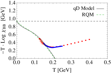
Figure 4: Plot of $-T\log|\chi_{BB}|$ as a function of temperature. We display as dots the lattice data from Refs. [5] (red) and [6] (blue). We also display the HRG model results including the spectrum of the $qD$ model (solid black), and the RQM spectrum [24] (dashed green).

where $M_{0}^{ab}$ is the mass of the lowest-lying state in the spectrum with quantum numbers $a$ and $b$. For the baryonic susceptibilities, these states are $M_{0}^{BB}=M_{0}^{BQ}=M_{p}$ the proton mass, and $M_{0}^{BS}=M_{\Lambda^{0}}$ the $\Lambda^{0}$ baryon mass. This observation, which goes beyond the HRG model as the lightest hadron saturates the QCD partition function in each sector at low enough temperature, makes it appealing to plot the lattice data for the susceptibilities in logarithmic scale. The corresponding plot for $\chi_{BB}$ is displayed in Fig. 4, and compared with the HRG approach including: i) the quark-diquark model spectrum computed in Sec. 3, and ii) the RQM baryon spectrum [24]. The horizontal dashed line represents the value of the lowest-lying state contributing to the fluctuation (the proton), cf. Eq. (27). In practice we find that at the lowest available temperatures, the contribution of excited states becomes individually small but collectively important. This is a typical problem in intermediate temperature analyses.

4.3 Baryonic susceptibilities with the $qD$ model spectrum

From the spectrum of the $qD$ model, we can obtain the baryonic susceptibilities by using the HRG approach given by Eq. (26). Since our goal is to reproduce the lowest temperature values of the lattice results for these quantities, we have chosen to minimize the function

$$\bar{\chi}^{2}=\bar{\chi}_{BB}^{2}+\bar{\chi}_{BQ}^{2}+\bar{\chi}_{BS}^{2}\,,\quad\textrm{where}\quad\bar{\chi}_{ab}^{2}=\sum_{j=1}^{j_{\max}}\frac{\left(\chi_{ab}^{{\textrm{\scriptsize lat}}}(T_{j})-\chi_{ab}^{\textrm{\tiny HRG}}(T_{j})\right)^{2}}{(\Delta\chi_{ab}^{{\textrm{\scriptsize lat}}}(T_{j}))^{2}}\,,$$ (28)

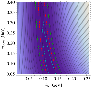
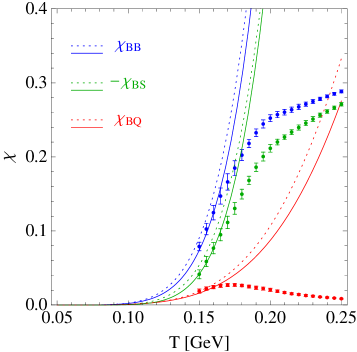
Figure 5: Left panel: $\bar{\chi}^{2}/\nu$ in the plane $(\hat{m}_{s},m_{{\textrm{\scriptsize cons}}})$ from a fit to the lattice data of the baryonic fluctuations from [6] with $T\leq 165\,{\rm MeV}$. The dashed lines correspond to $\bar{\chi}^{2}/\nu=0.77$ (curve delimiting a smaller area), $\bar{\chi}^{2}/\nu=1$, and $\bar{\chi}^{2}/\nu=1+\sqrt{2/\nu}$ (curve delimiting a larger area). Right panel: Baryonic susceptibilities from the quark-diquark model (solid) compared to the lattice data of Ref. [6]. We display also as dotted lines the results from the spectrum of the RQM [24]. For the quark-diquark model we have used the parameters in Eq. (21).

and $j_{\max}$ is the number of data points used in the fits. As explained in Sec. 3.2, the model contains three free parameters. We show in the left panel of Fig. 5 a plot of $\bar{\chi}^{2}/\nu$, where $\nu$ is the number of degrees of freedom, in the plane $(\hat{m}_{s},m_{{\textrm{\scriptsize cons}}})$.  One can observe from this figure that the current quark mass for the strange quark takes a value compatible with the PDG, i.e. $80\,{\rm MeV}\lesssim\hat{m_{s}}\lesssim 120\,{\rm MeV}$, while the constituent quark mass is in the range $100\,{\rm MeV}\lesssim m_{{\textrm{\scriptsize cons}}}\lesssim 400\,{\rm MeV}$. Based on these results, we propose the choice of the parameters of the model already presented in Eq. (21). Using them, we obtain the results for the baryonic susceptibilities that are displayed in the right panel of Fig. 5.

In some previous works, the Coulombic term of the $qD$ potential is regularized at the origin $(r=0)$ by adding a term of the form $\Delta V_{qQ}(r)=\tau e^{-\kappa r}/r$ in Eq. (15), see e.g. Refs. [31, 32]. To study the effects of this term, we have considered the following values for the regularization parameter: $\kappa=(10\,{\rm fm}^{-1},40\,{\rm fm}^{-1},80\,{\rm fm}^{-1})$. This range includes most of the values considered in the literature. Then we find that this correction increases the lowest states of the baryon spectrum by $\Delta m_{n}/m_{n}\sim~{}(0.7\%\,,0.05\%\,,0.015\%)$ for $\kappa=(10\,{\rm fm}^{-1},40\,{\rm fm}^{-1},80\,{\rm fm}^{-1})$, being this increase less important for heavier states. These effects in the spectrum induce small corrections in the baryonic susceptibilities that tend to decrease their absolute values by $|\delta\chi_{ab}^{{\textrm{\tiny HRG}}}|/|\chi_{ab}^{{\textrm{\tiny HRG}}}|\sim~{}(2\%,0.2\%,0.02\%)$ respectively, in the temperature regime $T\gtrsim 0.1\,{\rm GeV}$, which is the relevant one for the fits performed in the present work. 

4.4 Baryonic susceptibilities of higher order

Higher order fluctuations can be obtained within the HRG model by taking higher derivatives of the thermodynamical potential. The corresponding susceptibility of order $(p,q,r)$ in charges $(B,Q,S)$ reads

$$\chi^{BQS}_{pqr}(T) =\frac{\partial^{p+q+r}\left(p/T^{4}\right)}{(\partial\hat{\mu}_{B})^{p}(\partial\hat{\mu}_{Q})^{p}(\partial\hat{\mu}_{S})^{r}}\Bigg{|}_{\hat{\mu}_{a}=0}$$ (29)

$$=\frac{1}{2\pi^{2}}\sum_{i\in{\rm Hadrons}}g_{i}\,B_{i}^{p}Q_{i}^{q}S_{i}^{r}\;\sum_{n=1}^{\infty}\zeta_{i}^{n+1}n^{p+q+r-2}\,\frac{M_{i}^{2}}{T^{2}}K_{2}\!\left(\frac{nM_{i}}{T}\right)\,,$$

where $p=-\Omega/V$ is the pressure, and $\hat{\mu}_{a}=\mu_{a}/T$.  We have studied within the HRG approach some of the baryonic susceptibilities of fourth, sixth and eighth order, i.e. $p+q+r=4$, $6$ and $8$. The results, and their comparison to the lattice data, are displayed in Fig. 6. We find that the lattice data are well reproduced for $T\lesssim 160\,{\rm MeV}$. However, it can be noted that while the agreement is reasonable, these data are typically affected by larger error bars than those of the second order fluctuations studied above, and the behavior turns out to be noisier.

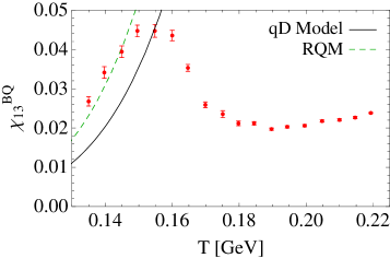
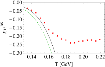
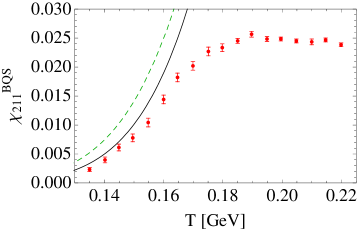
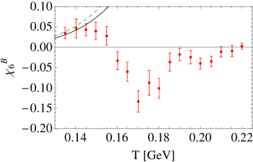
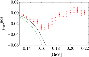
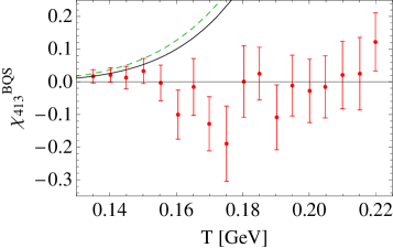
Figure 6: Baryonic susceptibilities of fourth order ($\chi_{13}^{BQ}$, $\chi_{13}^{BS}$, $\chi_{211}^{BQS}$), sixth order ($\chi_{6}^{B}$, $\chi_{312}^{BQS}$) and eighth order ($\chi_{413}^{BQS}$) from the quark-diquark model (solid black). We have used the parameters in Eq. (21). We display as dots the lattice data of Ref. [49], and as dashed (green) lines the results by using the HRG model with the baryonic spectrum of the RQM [24].

5 Semiclassical estimates of the baryonic susceptibilities

The computation of the $qD$ model spectrum in Sec. 3.3 has been performed by considering numerical methods for the solution of the quantum mechanical two body system. We will study in this section the spectrum and the baryonic susceptibilities within a semiclassical expansion, and provide some analytical formulas valid at high enough hadron masses and/or temperatures. While Eq. (26) is the basic formula that we will consider for the susceptibilities, we prefer to write it in the following form

$$\chi_{ab}(T)=\frac{1}{2\pi^{2}}\sum_{\zeta=\pm}\int_{0}^{\infty}dM\rho^{\zeta}_{ab}(M)\left(\frac{M}{T}\right)^{2}\sum_{k=1}^{\infty}\zeta^{k+1}K_{2}\left(\frac{kM}{T}\right)\,,$$ (30)

where

$$\rho^{\zeta}_{ab}(M)=\sum_{i}g_{i}\,q_{i}^{a}\,q_{i}^{b}\,\delta(M-M_{i})\,,$$ (31)

and the sum is over mesons or baryons for $\zeta=\pm 1$ respectively. Note that for the baryonic susceptibility $\chi_{BB}$, one has that $\rho_{BB}(M)$ is equal to the density of states $\rho(M)=dN(M)/dM$, as $B=\pm 1$ for (anti)baryons.

5.1 Semiclassical expansion

The spectrum of a quantum mechanical system, more specifically the density of states, can be computed in a derivative expansion, an approximation that is closely related to a semiclassical expansion (also called WKB method) in the high mass regime [35]. Within the WKB method, the leading contribution to the cumulative number writes

$$N(M)=\Tr(\Theta(M-\hat{H}))\simeq\int\frac{d^{3}xd^{3}p}{(2\pi)^{3}}\Theta(M-H)+\cdots\,,$$ (32)

where the (classical) Hamiltonian is given by 

$$H=\sqrt{{\mathbf{p}}^{2}+m_{q}^{2}}+\sqrt{{\mathbf{p}}^{2}+m_{D}^{2}}+\sigma r-\frac{4\alpha_{S}}{3r}+\mu\,.$$ (33)

The zeroth order term in Eq. (32) (which will be denoted by WKB₀) has been made explicit, while the dots stand for higher order contributions in the derivative expansion. The trace in the second equality of Eq. (32) is taken in the center of mass system subspace.

5.2 Massless quarks and diquarks

Let us consider first the case of massless quarks and diquarks, and treat the Coulomb term perturbatively, i.e. $H=H_{0}+H_{1}$ with

$$H_{0}=2p+\sigma r\,,\qquad H_{1}=-\frac{4\alpha_{S}}{3r}\,,$$ (34)

and $p=|{\mathbf{p}}|$. Using the Taylor expansion of the step function

$$\Theta(M-H)=\Theta(M-H_{0})-\delta(M-H_{0})H_{1}+\frac{1}{2}\delta^{\prime}(M-H_{0})H_{1}^{2}+\cdots\,,$$ (35)

and after performing the spatial and momentum integral of Eq. (32), one finds the following contribution of the cumulative number at leading order in the semiclassical expansion

$$N^{{\textrm{\tiny WKB}}_{0}}(M)=\frac{M^{6}}{720\pi\sigma^{3}}+\alpha_{S}\frac{M^{4}}{36\pi\sigma^{2}}+\alpha_{S}^{2}\frac{2M^{2}}{9\pi\sigma}+\cdots\,.$$ (36)

Plugging this result into Eq. (30) with $\zeta=-1$, one gets the baryonic susceptibility

$$\chi_{BB}^{{\textrm{\tiny WKB}}_{0}}(T)=\frac{127\pi^{5}}{94500}\left(\frac{T^{2}}{\sigma}\right)^{3}+\frac{31\pi^{3}}{5670}\alpha_{S}\left(\frac{T^{2}}{\sigma}\right)^{2}+\frac{7\pi}{405}\alpha_{S}^{2}\frac{T^{2}}{\sigma}+\cdots\,.$$ (37)

A factor of 2 has to be included to account for the antibaryons.

5.3 Finite mass effects

If $\alpha_{S}$ is set to zero, the integral in Eq. (32) can be computed analytically in the massive case by considering the following change of variable in the momentum integral

$$p\longrightarrow E:=\sqrt{p^{2}+m_{q}^{2}}+\sqrt{p^{2}+m_{D}^{2}}\,.$$ (38)

The result for the cumulative number turns out to be rather lengthy, but we can provide a shorter expression corresponding to the asymptotic limit of $M$ near and above the (classical) threshold $M_{\rm threshold}=m_{q}+m_{D}$, i.e.

$$N^{{\textrm{\tiny WKB}}_{0}}(M)=\frac{64\sqrt{2}}{945\pi\sigma^{3}}\left(\frac{m_{q}m_{D}}{m_{q}+m_{D}}\right)^{3/2}(M-m_{q}-m_{D})^{9/2}+\cdots\,.$$ (39)

This region dominates the behavior of the susceptibility at small temperatures, namely,

$$\chi_{BB}^{{\textrm{\tiny WKB}}_{0}}(T)=\frac{(m_{q}m_{D})^{3/2}T^{3}}{\pi^{2}\sigma^{3}}e^{-(m_{q}+m_{D})/T}+\cdots$$ (40)

for $T\ll m_{q}+m_{D}$. This temperature regime is appropriate for the values of $m_{q}$, $m_{D}$ and $T$ considered in this work. We display in Fig. 7 the result for the cumulative number and baryonic susceptibility computed with the WKB approximation presented above, and compared with the variational procedure of Sec. 3.3 and the lattice data of Ref. [6]. Notice that the WKB result correctly reproduces the baryon spectrum for masses $M\gtrsim 1500\,{\rm MeV}$.

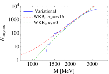
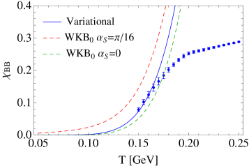
Figure 7: Left panel: Cumulative number of the spectrum of baryons with the quark-diquark model. Right panel: Baryonic $\chi_{BB}$ susceptibility obtained with that spectrum. We display as dashed lines the result from the WKB approximation at leading order. The points in the right panel are the lattice data of Ref. [6].

6 Conclusions

In the present work we have studied the baryon spectrum in the $(uds)$ flavor sector of QCD. We have argued that the asymptotic three-body phase space for confined $qqq$ systems $\sim M^{12}$ is much larger than the one actually observed in the PDG or determined in the RQM, $\sim M^{6}$. This resembles a two body confined system despite the fact that, by construction, baryons in the RQM are explicitly described as $qqq$ bound states. This strongly suggests a dynamics for excited baryons dominated by quark-diquark degrees of freedom, motivating the use of a quark-diquark model to compute the baryon spectrum. In a simplified version of the model hyperfine splittings are neglected and the pertinent quark-diquark potential is found to be identical to the quark-antiquark using the appropriate Polyakov loop correlators, and in strong agreement with lattice QCD determinations. The obtained baryon spectrum and its related baryonic susceptibilities in a thermal medium have been evaluated within the HRG approach and successfully fitted to lattice QCD data in terms of the constituent diquark mass and the current strange quark mass. The results fall in the bulk of previous intensive studies where a detailed description of the spectrum was pursued. The extension of our work to nonbaryonic susceptibilities would require a specific model for mesons. These and other issues will be addressed in a forthcoming publication [50].

References

References

- [1] Z. Citron et al., Report from Working Group 5 : Future physics opportunities for high-density QCD at the LHC with heavy-ion and proton beams, CERN Yellow Rep. Monogr. 7, 1159 (2019).
- [2] G. Odyniec [STAR Collaboration], Beam Energy Scan Program at RHIC (BES I and BES II) – Probing QCD Phase Diagram with Heavy-Ion Collisions, PoS CORFU 2018, 151 (2019).
- [3] P. Senger, The heavy-ion program of the future FAIR facility, J. Phys. Conf. Ser. 798, no. 1, 012062 (2017).
- [4] V. Kekelidze, A. Kovalenko, R. Lednicky, V. Matveev, I. Meshkov, A. Sorin and G. Trubnikov, Feasibility study of heavy-ion collision physics at NICA JINR, Nucl. Phys. A967, 884 (2017).
- [5] S. Borsanyi, Z. Fodor, S. D. Katz, S. Krieg, C. Ratti, K. Szabo, Fluctuations of conserved charges at finite temperature from lattice QCD, JHEP 01 (2012) 138.
- [6] A. Bazavov, et al., Fluctuations and Correlations of net baryon number, electric charge, and strangeness: A comparison of lattice QCD results with the hadron resonance gas model, Phys. Rev. D86 (2012) 034509.
- [7] G.y. Shao, Z.d. Tang, X.y. Gao and W.b. He, Baryon number fluctuations and the phase structure in the PNJL model, Eur. Phys. J. C78, no. 2, 138 (2018).
- [8] R. Wen, C. Huang and W. J. Fu, Baryon number fluctuations in the 2+1 flavor low energy effective model, Phys. Rev. D99, no. 9, 094019 (2019).
- [9] P. Isserstedt, M. Buballa, C. S. Fischer and P. J. Gunkel, Baryon number fluctuations in the QCD phase diagram from Dyson-Schwinger equations, Phys. Rev. D100, no. 7, 074011 (2019).
- [10] R. Hagedorn, Statistical thermodynamics of strong interactions at high-energies, Nuovo Cim. Suppl. 3 (1965) 147–186.
- [11] R. Hagedorn, How We Got to QCD Matter from the Hadron Side: 1984, Lect. Notes Phys. 221 (1985) 53–76.
- [12] M. Tanabashi, et al., Review of Particle Physics, Phys. Rev. D98 (3) (2018) 030001.
- [13] A. Miyahara, M. Ishii, H. Kouno and M. Yahiro, “A hadron-quark hybrid model reliable for the EoS in MeV,” arXiv:1907.07306 [hep-ph].
- [14] S. Borsanyi, Z. Fodor, C. Hoelbling, S. D. Katz, S. Krieg, K. K. Szabo, Full result for the QCD equation of state with 2+1 flavors, Phys. Lett. B730 (2014) 99–104.
- [15] A. Bazavov, et al., Equation of state in ( 2+1 )-flavor QCD, Phys. Rev. D90 (2014) 094503.
- [16] E. Ruiz Arriola, L.L. Salcedo, E. Megias, Quark Hadron Duality at Finite Temperature, Acta Phys. Polon. B45 (12) (2014) 2407–2454.
- [17] E. Ruiz Arriola, W. Broniowski, E. Megias, L.L. Salcedo, Thermal shifts, fluctuations, and missing states, Workshop on Excited Hyperons in QCD Thermodynamics at Freeze-Out (YSTAR2016) Mini-Proceedings (2016) 128–139. arXiv:1612.07091.
- [18] E. Megias, E. Ruiz Arriola, L.L. Salcedo, Thermodynamic characterizations of exotic and missing states, PoS Hadron2017 (2018) 232. arXiv:1711.09837.
- [19] E. Megias, E. Ruiz Arriola, L.L. Salcedo, Heavy quark-antiquark free energy and thermodynamics of string-hadron avoided crossings, Phys. Rev. D94 (9) (2016) 096010.
- [20] M. Asakawa, M. Kitazawa, Fluctuations of conserved charges in relativistic heavy ion collisions: An introduction, Prog. Part. Nucl. Phys. 90 (2016) 299–342.
- [21] H.-T. Ding, F. Karsch, S. Mukherjee, Thermodynamics of strong-interaction matter from Lattice QCD, Int. J. Mod. Phys. E24 (10) (2015) 1530007.
- [22] P. Huovinen, P. Petreczky, Hadron Resonance Gas with Repulsive Interactions and Fluctuations of Conserved Charges, Phys. Lett. B777 (2018) 125–130.
- [23] S. Godfrey, N. Isgur, Mesons in a Relativized Quark Model with Chromodynamics, Phys. Rev. D32 (1985) 189–231.
- [24] S. Capstick, N. Isgur, Baryons in a Relativized Quark Model with Chromodynamics, Phys. Rev. D34 (1986) 2809.
- [25] M. Anselmino, E. Predazzi, S. Ekelin, S. Fredriksson, D. B. Lichtenberg, Diquarks, Rev. Mod. Phys. 65 (1993) 1199–1234.
- [26] S. Fleck, B. Silvestre-Brac, J. M. Richard, Search for Diquark Clustering in Baryons, Phys. Rev. D38 (1988) 1519–1529.
- [27] E. Santopinto, An Interacting quark-diquark model of baryons, Phys. Rev. C72 (2005) 022201.
- [28] J. Ferretti, A. Vassallo, E. Santopinto, Relativistic quark-diquark model of baryons, Phys. Rev. C83 (2011) 065204.
- [29] M. De Sanctis, J. Ferretti, E. Santopinto, A. Vassallo, Electromagnetic form factors in the relativistic interacting quark-diquark model of baryons, Phys. Rev. C84 (2011) 055201.
- [30] G. Galata, E. Santopinto, Hybrid quark-diquark baryon model, Phys. Rev. C86 (2012) 045202.
- [31] E. Santopinto, J. Ferretti, Strange and nonstrange baryon spectra in the relativistic interacting quark-diquark model with a Gürsey and Radicati-inspired exchange interaction, Phys. Rev. C92 (2) (2015) 025202.
- [32] M. De Sanctis, J. Ferretti, E. Santopinto, A. Vassallo, Relativistic quark-diquark model of baryons with a spin-isospin transition interaction: Non-strange baryon spectrum and nucleon magnetic moments, Eur. Phys. J. A52 (5) (2016) 121.
- [33] C. Gutierrez, M. De Sanctis, A study of a relativistic quark-diquark model for the nucleon, Eur. Phys. J. A50 (11) (2014) 169.
- [34] C. Alexandrou, P. de Forcrand, B. Lucini, Evidence for diquarks in lattice QCD, Phys. Rev. Lett. 97 (2006) 222002.
- [35] J. Caro, E. Ruiz Arriola, L.L. Salcedo, Semiclassical expansions up to order h-bar**4 in relativistic nuclear physics, J. Phys. G22 (1996) 981–1011.
- [36] E. Ruiz Arriola, L.L. Salcedo, E. Megias, Excited Hadrons, Heavy Quarks and QCD thermodynamics, Acta Phys. Polon. Supp. 6 (3) (2013) 953–958.
- [37] E. Megias, E. Ruiz Arriola, L.L. Salcedo, The Hadron Resonance Gas Model: Thermodynamics of QCD and Polyakov Loop, Nucl. Phys. Proc. Suppl. 234 (2013) 313–316.
- [38] P. Masjuan, E. Ruiz Arriola, Regge trajectories of Excited Baryons, quark-diquark models and quark-hadron duality, Phys. Rev. D96 (5) (2017) 054006.
- [39] E. Ruiz Arriola, P. Masjuan, W. Broniowski, Excited Hadrons and Quark-Hadron Duality, Acta Phys. Polon. Supp. 10 (2017) 1079.
- [40] E. Megias, E. Ruiz Arriola, L.L. Salcedo, The Polyakov loop and the hadron resonance gas model, Phys. Rev. Lett. 109 (2012) 151601.
- [41] Y. Koma, M. Koma, Precise determination of the three-quark potential in SU(3) lattice gauge theory, Phys. Rev. D95 (9) (2017) 094513.
- [42] O. W. Greenberg, H. J. Lipkin, The Potential Model of Colored Quarks: Success for Single Hadron States, Failure for Hadron - Hadron Interactions, Nucl. Phys. A370 (1981) 349–364.
- [43] M. J. Savage, M. B. Wise, Spectrum of baryons with two heavy quarks, Phys. Lett. B248 (1990) 177–180.
- [44] E. Megias, E. Ruiz Arriola, L.L. Salcedo, Baryonic susceptibilities, quark-diquark models and quark-hadron duality at finite temperature, Phys. Rev. D99 (7) (2019) 074020.
- [45] R. L. Jaffe, Exotica, Phys. Rept. 409 (2005) 1–45.
- [46] E. Megias, E. Ruiz Arriola, L.L. Salcedo, Fluctuations and correlations in thermal QCD, Nucl. Part. Phys. Proc. 300-302 (2018) 196–202.
- [47] P. Huovinen, P. Petreczky, QCD Equation of State and Hadron Resonance Gas, Nucl. Phys. A837 (2010) 26–53.
- [48] E. Megias, E. Ruiz Arriola, L.L. Salcedo, Trace Anomaly, Thermal Power Corrections and Dimension Two condensates in the deconfined phase, Phys. Rev. D80 (2009) 056005.
- [49] S. Borsanyi, Z. Fodor, J. N. Guenther, S. K. Katz, K. K. Szabo, A. Pasztor, I. Portillo, C. Ratti, Higher order fluctuations and correlations of conserved charges from lattice QCD, JHEP 10 (2018) 205.
- [50] E. Megias, E. Ruiz Arriola, L.L. Salcedo, work in progress (2020).