AMP Chain Graphs: Minimal Separators
and Structure Learning Algorithms

Abstract

We address the problem of finding a minimal separator in an Andersson–Madigan–Perlman chain graph (AMP CG), namely, finding a set $Z$ of nodes that separates a given non-adjacent pair of nodes such that no proper subset of $Z$ separates that pair. We analyze several versions of this problem and offer polynomial time algorithms for each. These include finding a minimal separator from a restricted set of nodes, finding a minimal separator for two given disjoint sets, and testing whether a given separator is minimal. To address the problem of learning the structure of AMP CGs from data, we show that the PC-like algorithm (Peña, 2012) is order-dependent, in the sense that the output can depend on the order in which the variables are given. We propose several modifications of the PC-like algorithm that remove part or all of this order-dependence. We also extend the decomposition-based approach for learning Bayesian networks (BNs) proposed by (Xie et al., 2006) to learn AMP CGs, which include BNs as a special case, under the faithfulness assumption. We prove the correctness of our extension using the minimal separator results. Using standard benchmarks and synthetically generated models and data in our experiments demonstrate the competitive performance of our decomposition-based method, called LCD-AMP, in comparison with the (modified versions of) PC-like algorithm. The LCD-AMP algorithm usually outperforms the PC-like algorithm, and our modifications of the PC-like algorithm learn structures that are more similar to the underlying ground truth graphs than the original PC-like algorithm, especially in high-dimensional settings. In particular, we empirically show that the results of both algorithms are more accurate and stabler when the sample size is reasonably large and the underlying graph is sparse.

Keywords: AMP chain graph, conditional independence, decomposition, separator, junction tree, augmented graph, triangulation, graphical model, Markov equivalent, structural learning.

1 Introduction

Probabilistic graphical models (PGMs), and their use for reasoning intelligently under uncertainty, emerged in the 1980s within the statistical and artificial intelligence reasoning communities. Probabilistic graphical models are now widely accepted as a powerful and mature tools for reasoning under uncertainty. Unlike some of the ad hoc approaches taken in early experts systems, PGMs are based on the strong mathematical foundations of graph and probability theory. In fact, any PGM consists of two main components: (1) a graph that defines the structure of the model; and (2) a joint distribution over random variables of the model. The main advantages of using PGMs compared to other models are that the representation is intuitive, inference can often be done efficiently and practical learning algorithms exist.  This led PGMs to become arguably the most important architecture for reasoning with uncertainty in artificial intelligence (Koller and Friedman, 2009; Neapolitan and Jiang, 2018). There are many efficient algorithms for both inference and learning available in open-source (Højsgaard et al., 2012; Nagarajan et al., 2013; Scutari and Denis, 2015) and commercial software (Hugin, Netica, GeNIe, and BayesiaLab). Moreover, their power and efficacy has been proven through their successful application to an enormous range of real-world problem domains. They can be used for a wide range of reasoning tasks including prediction, monitoring, diagnosis, risk assessment and decision making (Spirtes et al., 2000; Xiang, 2002; Jensen and Nielsen, 2007; Fenton and Neil, 2018).

One of the most basic subclasses of PGMs is Markov networks. The graphical framework of Markov networks are undirected graphs (UGs), in which each undirected edge represents a symmetric relation i.e., direct correlation between the two variables it connects, while no edge means that the variables are not directly correlated. The best known and most widely used PGM class, however, is Bayesian networks. The graphical structures of Bayesian networks are directed acyclic graphs (DAGs). In a DAG the directed edges can often be seen as representing cause and effect (asymmetric) relationships e.g., see (Motzek and Möller, 2017).

Chain graphs (CGs) were introduced as a unification of directed and undirected graphs to model systems containing both symmetric and asymmetric relations. In fact, a chain graph is a type of mixed graph, admitting both directed and undirected edges, which contain no partially directed cycles. So, CGs may contain two types of edges, the directed type that corresponds to the causal relationship in DAGs and a second type of edge representing a symmetric relationship (Sonntag, 2016). In particular, $X_{1}$ is a direct cause of $X_{2}$ only if $X_{1}\to X_{2}$ (i.e., $X_{1}$ is a parent of $X_{2}$), and $X_{1}$ is a (possibly indirect) cause of $X_{2}$ only if there is a directed path from $X_{1}$ to $X_{2}$ (i.e., $X_{1}$ is an ancestor of $X_{2}$). So, while the interpretation of the directed edge in a CG is quite clear, the second type of edge can represent different types of relations and, depending on how we interpret it in the graph, we say that we have different CG interpretations with different separation criteria, i.e. different ways of reading conditional independences from the graph, and different intuitive meaning behind their edges. The three following interpretations are the best known in the literature. The first interpretation (LWF) was introduced by Lauritzen, Wermuth and Frydenberg (Lauritzen and Wermuth, 1989; Frydenberg, 1990) to combine DAGs and undirected graphs (UGs). The second interpretation (AMP), was introduced by Andersson, Madigan and Perlman, and also combines DAGs and UGs but with a Markov equivalence criterion that more closely resembles the one of DAGs (Andersson et al., 1996). The third interpretation, the multivariate regression interpretation (MVR), was introduced by Cox and Wermuth (Cox and Wermuth, 1993, 1996) to combine DAGs and bidirected (covariance) graphs.

This paper deals with chain graphs under the alternative Andersson-Madigan-Perlman (AMP) interpretation (Andersson et al., 1996, 2001). AMP CGs are useful when we have a set of variables for which the internal relations has no causal ordering, so the relations should be modelled as a Markov network, but also a second set of variables that can be seen as causes for some of these variables in the first set. The internal structure of the first set of variables can then be modelled as a Markov network, creating a chain component in an AMP CG, and the causes as parents of some of the variables in the chain component. Note that for AMP CGs the parents only affect the direct children in the chain component, not all the nodes in the chain component as in the case of LWF CGs. An example in medicine (Sonntag and Peña, 2015) when such a model might be appropriate is when we are modelling pain levels on different areas on the body of a patient. The pain levels can then be seen as correlated “geographically” over the body, and hence be modelled as a Markov network. Certain other factors do, however, exist that alters the pain levels locally at some of these areas, such as the type of body part the area is located on or if local anaesthetic has been administered in that area and so on. These outside factors can then be modeled as parents affecting the pain levels locally. AMP chain graphs are widely studied in different areas from applications in biology (Sonntag and Peña, 2015), to more advanced theoretical investigations (Richardson, 1998; Levitz et al., 2001; Roverato, 2005; Roverato and Rocca, 2006; Drton, 2009; Studený et al., 2009; Peña, 2014b, 2015; Sonntag and Peña, 2015; Peña, 2016; Peña and Gómez-Olmedo, 2016; Peña, 2018a, b).

Minimality is a desirable property to ensure efficiency and usability e.g., see (Peña, 2011). Finding minimal separators is useful for learning and inference tasks (Acid and de Campos, 1996; Javidian and Valtorta, 2019). Of course, finding these sets will take some effort, but the additional effort will be compensated by decreased computing time when using the corresponding independencies in learning and inference. Moreover, it will also increase the reliability of the results, because fewer data are needed to reliably compute a conditional dependence measure of lower order. For example, Acid and de Campos (Acid and de Campos, 2001) proposed a hybrid algorithm for learning Bayesian networks from data that uses minimal d-separators. They showed that the use of minimal $d$-separating sets is clearly useful, not only with respect to the quality of the learned network but also in terms of time complexity of the proposed algorithm. In this paper, we address the problem of finding minimal separators in AMP chain graphs and their applications in learning the structure of AMP CGs from data.

One important aspect of PGMs is the possibility of learning the structure of models directly from sampled data. Two constraint-based learning algorithms, that use a statistical analysis to test the presence of a conditional independency, exist for learning AMP CGs: (1) the PC-like algorithm (Peña, 2012; Peña and Gómez-Olmedo, 2016), and (2) the answer set programming (ASP) algorithm (Peña, 2016). In this paper, we show that the PC-like algorithm is order-dependent, in the sense that the output can depend on the order in which the variables are given. We propose several modifications of the PC-like algorithm, i.e., Stable PC-like for AMP CGs (Stable-PC4AMP), Conservative PC-like for AMP CGs (Conservative-PC4AMP), and a version that is both Stable and Conservative (Stable-Conservative-PC4AMP) for learning the structure of AMP chain graphs under the faithfulness assumption that remove part or all of the order-dependence.

(a) Observational Data

(b) Undirected Independence Graph Recovery

(c) Triangulation

(d) $p$-Separation Tree

(e) Local Skeleton Recovery

(f) Global Skeleton Recovery

(g) AMP CG Recovery

(h) Largest Deflagged Graph Recovery

Figure 1: An overview of LCD-AMP ’s steps for learning the structure of the largest deflagged AMP CG from a faithful distribution.

We use some of our findings regarding minimal separators in AMP CGs to prove the correctness of a new efficient algorithm for learning AMP chain graphs, called Learn Chain graphs via Decomposition for AMP CGs (LCD-AMP). Our proposed LCD-AMP algorithm, illustrated in Figure 1, consists of five steps: (1) An undirected graphical model for the data is chosen. Any conditional independencies that hold under this model will also hold under the selected chain graph, so this step serves to restrict the search space in the third step. (2) A junction tree as a facilitator for decomposition of structure learning is built from the triangulated graph obtained from the resulting graph at the end of step (1). (3) Local skeletons are recovered in each individual node of the obtained separation tree from the previous step. (4) The global skeleton is recovered by merging recovered local skeletons from the previous step along with removing those edges that are deleted in any local skeleton. (5) Arrowheads are added to some of the edges to obtain desired AMP chain graph. The details of each step with related definitions are provided later in the paper (Section 5). This algorithm not only reduces complexity and increases the power of computational independence tests but also achieves a better quality with respect to the learned structure.

The results of the experiments show that our proposed algorithm Learn Chain graphs via Decomposition for AMP interpretation (LCD-AMP) consistently outperforms the ( Stable-) PC-like algorithm. Our proposed algorithms, i.e., the Stable PC-like for AMP CGs (Stable-PC4AMP) and LCD-AMP  are able to exploit the parallel computations for scaling up the task of learning AMP chain graphs. This will enable AMP chain graph discovery on large datasets. In fact, lower complexity, higher power of computational independence test, better learned structure quality, along with the ability of exploiting parallel computing, make our proposed algorithms more desirable and suitable for big data analysis when AMP chain graphs are being used. Code for reproducing our results is available at https://github.com/majavid/AMPCGs2019.

Our main contributions are the following:

1. We propose several polynomial time algorithms to solve the problem of finding minimal separating sets in AMP chain graphs (Section 3).

2. We show that the original PC-like algorithm (Peña, 2012) is order-dependent, in the sense that the output can depend on the order in which the variables are given. Then, we propose modifications of the PC-like algorithm, i.e., Stable PC-like for AMP (Stable-PC4AMP), Conservative PC-like for AMP (Conservative-PC4AMP), and Stable-Conservative-PC4AMP for learning the structure of AMP chain graphs under the faithfulness assumption that remove part or all of the order-dependence (Section 4).

3. We present a computationally feasible algorithm for learning the structure of AMP chain graphs via decomposition, called LCD-AMP , that reduces complexity and increase the power of computational independence tests (Section 5).

4. We compare the performance of our algorithms with that of the PC-like algorithm proposed in (Peña, 2012), in the Gaussian and discrete cases. We empirically show that our modifications of the PC-like algorithm achieve output of better quality than the original PC-like algorithm, especially in high-dimensional settings. We also show that our decomposition based algorithm, i.e., the LCD-AMP algorithm outperforms the ( Stable-) PC-like algorithm in our experiments (Section 6).

5. We release supplementary material including data and an R package that implements the proposed algorithms.

2 Basic Definitions and Concepts

In this paper, we consider graphs containing both directed (of the form $a\to b$ or, simply, $(a,b)$) and undirected (of the form $a-b$ or, simply, $\{a,b\}$) edges and largely use the terminology of (Andersson et al., 2001), where the reader can also find further details. Below we briefly list some of the central concepts used in this paper.

If $A\subseteq V$ is a subset of the vertex set in a graph $G=(V,E)$, the induced subgraph $G_{A}=(A,E_{A})$ is a graph in which the edge set $E_{A}=E\cap(A\times A)$ is obtained from $G$ by keeping edges with both endpoints in $A$.

If there is an arrow from $a$ pointing towards $b$, $a$ is said to be a parent of $b$. The set of parents of $b$ is denoted as $pa(b)$. If there is an undirected edge between $a$ and $b$, $a$ and $b$ are said to be adjacent or neighbors. The set of neighbors of a vertex $a$ is denoted as $ne(a)$. The expressions $pa(A)$ and $ne(A)$ denote the collection of parents and neighbors of vertices in $A$ that are not themselves elements of $A$. The boundary $bd(A)$ of a subset $A$ of vertices is the set of vertices in $V\setminus A$ that are parents or neighbors to vertices in $A$. The closure of $A$ is $cl(A)=bd(A)\cup A$.

A directed path of length $n$ from $a$ to $b$ is a sequence $a=a_{0},\dots,a_{n}=b$ of distinct vertices such that $(a_{i},a_{i+1})\in E$, for all $i=0,\dots,n-1$. (A semidirected path of length $n$ from $a$ to $b$ is a sequence $a=a_{0},\dots,a_{n}=b$ of distinct vertices such that either $(a_{i},a_{i+1})$ or $\{a_{i},a_{i+1}\}\in E$, for all $i=0,\dots,n-1$.) A chain of length $n$ from $a$ to $b$ is a sequence $a=a_{0},\dots,a_{n}=b$ of distinct vertices such that $(a_{i},a_{i+1})\in E$, or $(a_{i+1},a_{i})\in E$, or $\{a_{i},a_{i+1}\}\in E$, for all $i=0,\dots,n-1$. A vertex $\alpha$ is said to be an ancestor of a vertex $\beta$ if there is a directed path $\alpha\to\dots\to\beta$ from $\alpha$ to $\beta$. We define the smallest ancestral set containing $A$ as $An(A):=an(A)\cup A$. A vertex $\alpha$ is said to be anterior to a vertex $\beta$ if there is a chain $\mu$ from $\alpha$ to $\beta$ on which every edge is either of the form $\gamma-\delta$, or $\gamma\to\delta$ with $\delta$ between $\gamma$ and $\beta$, or $\alpha=\beta$; that is, there are no edges $\gamma\leftarrow\delta$ pointing toward $\alpha$. We apply this definition to sets: $ant(X)=\{\alpha|\alpha\textrm{ is an anterior of }\beta\textrm{ for some }\beta\in X\}$.

A partially directed cycle (or semi-directed cycle) in a graph $G$ is a sequence of $n$ distinct vertices $v_{1},v_{2},\dots,v_{n}(n\geq 3)$, and $v_{n+1}\equiv v_{1}$, such that

(a) for all $i(1\leq i\leq n)$ either $v_{i}-v_{i+1}$ or $v_{i}\to v_{i+1}$, and

(b) there exists a $j(1\leq j\leq n)$ such that $v_{j}\to v_{j+1}$.

An AMP chain graph is a graph in which there are no partially directed cycles. The chain components $\mathcal{T}$ of a chain graph are the connected components of the undirected graph obtained by removing all directed edges from the chain graph. We define the smallest coherent set containing $A$ as $Co(A):=\cup_{\tau}\{\tau\in\mathcal{T}|\tau\cap A\neq\emptyset\}$. Let $\overline{G}$ be obtained by deleting all directed edges of $G$; for $A\subseteq V$ the extended subgraph G[A] is defined by $G[A]:=G_{An(A)}\cup\overline{G}_{Co(An(A))}$.

A triple of vertices $\{X,Y,Z\}$ is said to form a flag in CG if the induced subgraph $CG_{X\cup Y\cup Z}$ is $X\to Y-Z$ or $X-Y\leftarrow Z$. A triple of vertices $\{X,Y,Z\}$ is said to form a triplex in CG if the induced subgraph $CG_{X\cup Y\cup Z}$ is either $X\to Y-Z$, $X\to Y\leftarrow Z$, or $X-Y\leftarrow Z$. A triplex is augmented by adding the $X-Z$ edge. A set of four vertices $\{X,A,B,Y\}$ is said to form a bi-flag if the edges $X\to A$, $Y\to B$, and $A-B$ are present in the induced subgraph over $\{X,A,B,Y\}$. A bi-flag is augmented by adding the edge $X-Y$. A minimal complex (or simply a complex) in a chain graph is an induced subgraph of the form $a\to v_{1}-\cdots\cdots-v_{r}\leftarrow b$. The augmented CG $G^{a}$ is the undirected graph formed by augmenting all triplexes and bi-flags in CG and replacing all directed edges with undirected edges (see Fig. 2). The skeleton (underlying graph) of a CG $G$ is obtained from $G$ by changing all directed edges of $G$ into undirected edges. Vertex $Y$ is an unshielded collider (or V-structure) in a DAG $G$ if $G$ contains the induced subgraph $U\to Y\leftarrow V$.

Figure 2: (a) Triplexes and (b) the corresponding augmented triplex, (c) the four configurations that define the bi-flag; (d) the corresponding augmented bi-flag. The “?” indicates that either $X-Y\in G$, $X\to Y\in G$, $Y\to X\in G$, or $X$ and $Y$ are not adjacent in $G$.

Definition 1

(Global Markov property for AMP chain graphs) For any triple $(A,B,S)$ of disjoint subsets of $V$ such that $S$ separates $A$ from $B$ in $(G[A\cup B\cup S])^{a}$, in the augmented graph of the extended subgraph of $A\cup B\cup S$, we have $A\!\perp\!\!\!\perp B|S$ (or $\langle A,B|S\rangle$) i.e., $A$ is independent of $B$ given $S$.

An equivalent pathwise separation criterion that identifies all valid conditional independencies under the AMP Markov property was introduced in (Levitz et al., 2001):

Definition 2

(The pathwise $p$-separation criterion for AMP chain graphs) A node $B$ in a chain $\rho$ in an AMP CG $G$ is called a triplex node in $\rho$ if $A\to B\leftarrow C,A\to B-C,\textrm{ or }A-B\leftarrow C$ is a subchain of $\rho$. Moreover, $\rho$ is said to be $Z$-open with $Z\subseteq V$ when

• every triplex node in $\rho$ is in $An(Z)$, and

• every non-triplex node $B$ in $\rho$ is outside $Z$, unless $A-B-C$ is a subchain of $\rho$ and $pa_{G}(B)\setminus Z\neq\emptyset$.

Let $X,Y\neq\emptyset$ and $Z$ (may be empty) denote three disjoint subsets of $V$. When there is no Z-open chain in an AMP CG $G$ between a node in $X$ and a node in $Y$, we say that $X$ is separated from $Y$ given $Z$ in $G$ and denote it as $X\!\perp\!\!\!\perp Y|Z$.

Theorem 4.1 in (Levitz et al., 2001) establishes the equivalence of the p-separation criterion and the augmentation criterion occurring in the AMP global Markov property for CGs.

Example 1

Consider the AMP CG $G$ in Fig. 3(a). The global Markov property of AMP chain graphs implies that $X\!\perp\!\!\!\perp Y|A$ (see Fig. 3). There is no A-open chain in the AMP CG $G$ between $X$ and $Y$ because the only chain between $X$ and $Y$ i.e., $X\to A-B\leftarrow Y$ is blocked at $B$ $(B\textrm{ is a triplex node in the chain and }B\not\in An(A))$.

Figure 3: (a) The AMP CG $G$, (b) $An(X\cup Y\cup A)$, (c) the undirected edges in $Co(An(X\cup Y\cup A))$, (d) $G[X\cup Y\cup A]$, and (e) $(G[X\cup Y\cup A])^{a}$.

We say that two AMP CGs $G$ and $H$ are Markov equivalent or that they are in the same Markov equivalence class if they induce the same conditional independence restrictions. Two chain graphs $G$ and $H$ are Markov equivalent if and only if they have the same skeletons and the same triplexes (Andersson et al., 2001). Two LWF chain graphs $G$ and $H$ are Markov equivalent if and only if they have the same skeletons and the same minimal complexes (Frydenberg, 1990). Two DAGs $G$ and $H$ are Markov equivalent if and only if they have the same skeletons and the same unshielded colliders (Pearl, 1988). The condition for AMP Markov equivalence of CGs more closely resembles that for DAG Markov equivalence than does the condition for LWF Markov equivalence of CGs, in the sense that triplexes involve only three vertices, while complexes can involve arbitrarily many vertices.

We say that AMP chain graphs $G$ and $H$ belong to the same strong Markov equivalent class iff $G$ and $H$ are Markov equivalent and contain the same flags. An AMP CG $G^{*}$ is said to be the AMP essential graph of its Markov equivalence class iff for every directed edge $A\to B$ that exists in $G^{*}$ there exists no AMP CG $H$ s.t. $G^{*}$ and $H$ are Markov equivalent and $A\leftarrow B$ is in $H$. An AMP CG $G^{*}$ is said to be the largest deflagged graph of its Markov equivalence class iff there exists no other AMP CG $H$ s.t. $G^{*}$ and $H$ are Markov equivalent and either $H$ contains fewer flags than $G^{*}$ or $G^{*}$ and $H$ belong to the same strong Markov equivalence class but $H$ contains more undirected edges. Any largest deflagged graph or AMP essential graph are AMP CGs and both of these have been proven to be unique for the Markov equivalence class they represent (Roverato and Rocca, 2006; Andersson and Perlman, 2006).

Let $\bar{G}_{V}=(V,\bar{E}_{V})$ denote an undirected graph where $\bar{E}_{V}$ is a set of undirected edges. For a subset $A$ of $V$, let $\bar{G}_{A}=(A,\bar{E}_{A})$ be the subgraph induced by $A$ and $\bar{E}_{A}=\{e\in\bar{E}_{V}|e\in A\times A\}=\bar{E}_{V}\cap(A\times A)$. An undirected graph is called complete if any pair of vertices is connected by an edge. For an undirected graph, we say that vertices $u$ and $v$ are separated by a set of vertices $Z$ if each path between $u$ and $v$ passes through $Z$. We say that two distinct vertex sets $X$ and $Y$ are separated by $Z$ if and only if $Z$ separates every pair of vertices $u$ and $v$ for any $u\in X$ and $v\in Y$. We say that an undirected graph $\bar{G}_{V}$ is an undirected independence graph (UIG) for CG $G$ if the fact that a set $Z$ separates $X$ and $Y$ in $\bar{G}_{V}$ implies that $Z$ $p$-separates $X$ and $Y$ in $G$. Note that the augmented graph derived from CG $G$, $(G)^{a}$, is an undirected independence graph for $G$. We say that $\bar{G}_{V}$ can be decomposed into subgraphs $\bar{G}_{A}$ and $\bar{G}_{B}$ if

• $A\cup B=V$, and

• $C=A\cap B$ separates $V\setminus A$ and $V\setminus B$ in $\bar{G}_{V}$.

The above decomposition does not require that the separator $C$ be complete, which is required for weak decomposition defined in (Lauritzen, 1996). In this paper, we show that a problem of learning the structure of CG can also be decomposed into problems for its decomposed subgraphs even if the separator is not complete.

A triangulated (chordal) graph is an undirected graph in which all cycles of four or more vertices have a chord, which is an edge that is not part of the cycle but connects two vertices of the cycle (see, for example, Figure 4). For an undirected graph $\bar{G}_{V}$ which is not triangulated, we can add extra (“fill-in”) edges to it such that it becomes a triangulated graph, denoted by $\bar{G}_{V}^{t}$.

Figure 4: (a) An AMP CG $G$. (b) The augmented graph $G^{a}$, which is also an undirected independence graph. (c) The triangulated graph $(G^{a})^{t}$.

In this paper, we assume that all independencies of a probability distribution of variables in $V$ can be checked by $p$-separations of $G$, called the faithfulness assumption (Spirtes et al., 2000). The faithfulness assumption means that all independencies and conditional independencies among variables can be represented by $G$.

The global skeleton is an undirected graph obtained by dropping direction of CG. A local skeleton for a subset $A$ of variables is an undirected subgraph for $A$ in which the absence of an edge $u\mathrel{\leavevmode\hbox to14.63pt{\vbox to0.4pt{\text{[drawing]}}}}v$ implies that there is a subset $S$ of $A$ such that $u\!\perp\!\!\!\perp v|S$. Now, we introduce the notion of $p$-separation trees, which is used to facilitate the representation of the decomposition. The concept is similar to the junction tree of cliques and the independence tree introduced for DAGs as $d$-separation trees in (Xie et al., 2006). Let $C=\{C_{1},\dots,C_{H}\}$ be a collection of distinct variable sets such that for $h=1,\dots,H,C_{h}\subseteq V$. Let $T$ be a tree where each node corresponds to a distinct variable set in $C$, to be displayed as an oval (see, for example, Figure 5). An undirected edge $e=\{C_{i},C_{j}\}$ connecting nodes $C_{i}$ and $C_{j}$ in $T$ is labeled with a separator $S=C_{i}\cap C_{j}$, which is displayed as a rectangle. Removing an edge $e$ or, equivalently, removing a separator $S$ from $T$ splits $T$ into two subtrees $T_{1}$ and $T_{2}$ with node sets $C_{1}$ and $C_{2}$ respectively. We use $V_{i}$ to denote the union of the vertices contained in the nodes of the subtree $T_{i}$ for $i=1,2$.

Figure 5: The $p$-separation tree of CG $G$ in Figure 4.

Notice that a separator is defined in terms of a tree whose nodes consist of variable sets, while the $p$-separator is defined based on chain graph. In general, these two concepts are not related, though for a $p$-separation tree its separator must be some corresponding $p$-separator in the underlying AMP chain graph. The definition of $p$-separation trees for AMP chain graphs is similar to that of junction trees of cliques, see (Cowell et al., 1999; Lauritzen, 1996). Actually, it is not difficult to see that a junction tree of chain graph $G$ is also a $p$-separation tree. However, as in (Ma et al., 2008), we point out two differences here: (a) a $p$-separation tree is defined with $p$-separation and it does not require that every node be a clique or that every separator be complete on the augmented graph; (b) junction trees are mostly used in inference engines, while our interest in $p$-separation trees is mainly derived from their power in facilitating the decomposition of structural learning.

Given an undirected graph $G=(V,E)$, a subset $S\subseteq V$ that does not contain $a$ or $b$ is said to be an $(a,b)$-separator if all paths from $a$ to $b$ intersect $S$. A set $S$ of nodes that separates a given pair of nodes such that no proper subset of $S$ separates that pair is called a minimal separator. Note that removing an $(a,b)$-separator disconnects a graph into two connected components, one containing $a$, and another containing $b$. Conversely, if a set $S$ disconnects a graph into a connected component including $a$ and another connected component including $b$, then $S$ is an $(a,b)$-separator. Two disjoint vertex subsets $A$ and $B$ of $V$ are adjacent if there is at least one pair of adjacent vertices $u\in A$ and $v\in B$. Let $A$ and $B$ be two disjoint non-adjacent subsets of $V$. Similarly, we define an $(A,B)$-separator to be any subset of $V\setminus(A\cup B)$ whose removal separates $A$ and $B$ in distinct connected components. A minimal $(A,B)$-separator does not contain any other $(A,B)$-separator.

3 Finding Minimal Separators in AMP Chain Graphs

In this section we propose and solve an optimization problem related to the separation in AMP chain graphs. The basic problem is formulated as follows: given a pair of non-adjacent nodes, $x$ and $y$, in an AMP chain graph, $G$, find a minimal set of nodes that separates $x$ and $y$. We analyze several versions of this problem and offer polynomial time algorithms for each. Apart from the possible theoretical interest that these problems may have (Tian et al., 1998; Acid and de Campos, 1996), generally, the solution to the basic problem (Problem 2) represents the minimum information i.e., minimal set of variables, whose values we have to know in order to break the mutual influence between two sets of variables, either in the absence of any other information (Problem 5, 6), or in the presence of some previous knowledge (Problem 1, 3, 4). These include the following problems:

Problem 1

(test for minimal separation) Given two non-adjacent nodes $X$ and $Y$ in an AMP chain graph $G$ and a set $Z$ that separates $X$ from $Y$, test if $Z$ is minimal i.e., no proper subset of $Z$ separates $X$ from $Y$.

Problem 2

(minimal separation) Given two non-adjacent nodes $X$ and $Y$ in an AMP chain graph $G$, find a minimal separating set between $X$ and $Y$, namely, find a set $Z$ such that $Z$, and no proper subset of $Z$, separates $X$ from $Y$.

Problem 3

(restricted separation) Given two non-adjacent nodes $X$ and $Y$ in an AMP chain graph $G$ and a set $S$ of nodes not containing $X$ and $Y$, find a subset $Z$ of $S$ that separates $X$ from $Y$.

Problem 4

(restricted minimal separation) Given two non-adjacent nodes $X$ and $Y$ in an AMP chain graph $G$ and a set $S$ of nodes not containing $X$ and $Y$, find a subset $Z$ of $S$ which is minimal and separates $X$ from $Y$.

Problem 5

(minimal separation of two disjoint non-adjacent sets) Given two disjoint non-adjacent sets $X$ and $Y$ in an AMP chain graph $G$, find a minimal separating set between $X$ and $Y$, namely, find a set $Z$ such that $Z$, and no proper subset of $Z$, separates $X$ from $Y$.

Problem 6

(enumeration of all minimal separators) Given two non-adjacent nodes (or disjoint subsets) $X$ and $Y$ in an AMP chain graph $G$, enumerate all minimal separating sets between $X$ and $Y$.

We prove that it is possible to transform our problem into a separation problem, where the undirected graph in which we have to look for the minimal set separating $X$ from $Y$ depends only on $X$ and $Y$. For each above mentioned problem, we propose and analyze an algorithm that, taking into account the previous results, solves it.

3.1 Main Theorem: Minimal Separators in AMP Chain Graphs

In this subsection we prove that it is possible to transform our problem into a separation problem, where the undirected graph in which we have to look for the minimal set separating $X$ from $Y$ depends only on $X$ and $Y$. Later, in the next subsections, we will apply this result to developing an efficient algorithm that solves our problems.

The next proposition shows that if we want to test a separation relationship between two disjoint sets of nodes $X$ and $Y$ in an AMP chain graph, where the separating set is included in the anterior set of $X\cup Y$, then we can test this relationship in a smaller AMP chain graph, whose set of nodes is formed only by the anteriors of $X$ and $Y$.

Proposition 3

Given an AMP chain graph $G=(V,E)$. Consider that $X,Y,$ and $Z$ are three disjoint subsets of $V,$ $Z\subseteq ant(X\cup Y)$, and $H=G_{ant(X\cup Y)}$ is the subgraph of $G$ induced by $ant(X\cup Y)$. Then ${\langle X,Y|Z\rangle}_{G}\Leftrightarrow{\langle X,Y|Z\rangle}_{H}.$

Proof  ($\Rightarrow$) The necessary condition is obvious, because a separator in a graph is also a separator in all of its subgraphs.

($\Leftarrow$) Since $bd(ant(X\cup Y))=\emptyset$, so $Co(An(ant(X\cup Y)))=ant(X\cup Y)$. Let ${\langle X,Y|Z\rangle}_{H}$ and $Z\subseteq ant(X\cup Y)$, then $Co(An(X\cup Y\cup Z))\subseteq ant(X\cup Y)$. Consider that ${\langle X,Y\not|Z\rangle}_{G}$. This means that $X$ is not separated from $Y$ given $Z$ in $(G[X\cup Y\cup Z])^{a}$, which is a subgraph of $(G[ant(X\cup Y)])^{a}$. In other words, there is a chain $C$ between $X$ and $Y$ in $H^{a}=(G[ant(X\cup Y)])^{a}=(G_{ant(X\cup Y)})^{a}$ that bypasses $Z$. Once again using $Z\subseteq ant(X\cup Y)$, we obtain that $X$ and $Y$ are not separated by $Z$ in $H$, in contradiction to the assumption ${\langle X,Y|Z\rangle}_{H}$. Therefore, it has to be ${\langle X,Y|Z\rangle}_{G}$.  

The following proposition establishes the basic result necessary to solve our optimization problems.

Proposition 4

Given an AMP chain graph $G=(V,E)$. Consider that $X,Y,$ and $Z$ are three disjoint subsets of $V$ such that ${\langle X,Y|Z\rangle}$ and ${\langle X,Y\not|Z^{\prime}\rangle},\forall Z^{\prime}\subsetneq Z$. Then $Z\subseteq ant(X\cup Y).$

Proof  Suppose that $Z\not\subseteq ant(X\cup Y)$. Define $Z^{\prime}=Z\cap ant(X\cup Y)$. Then, by assumption we have ${\langle X,Y\not|Z^{\prime}\rangle}$. Since $Z^{\prime}\subseteq ant(X\cup Y)$, it is obvious that $Co(An(X\cup Y\cup Z^{\prime}))\subseteq ant(X\cup Y)$. So, $X$ and $Y$ are not separated by $Z^{\prime}$ in $(G[X\cup Y\cup Z^{\prime}])^{a}$, hence there is a chain $C$ between $X$ and $Y$ in $(G[X\cup Y\cup Z^{\prime}])^{a}$ that bypasses $Z^{\prime}$ i.e., the chain $C$ is formed from nodes in $ant(X\cup Y)$ that are outside of $Z$. Since $Co(An(X\cup Y\cup Z^{\prime}))\subseteq ant(X\cup Y)$, then $(G[X\cup Y\cup Z^{\prime}])^{a}$ is a subgraph of $(G[ant(X\cup Y)])^{a}$. Then, the previously found chain $C$ is also a chain in $(G[ant(X\cup Y)])^{a}$ that bypasses $Z$, which means that $X$ and $Y$ are not separated by $Z$ in $(G[ant(X\cup Y)])^{a}=(G_{ant(X\cup Y)})^{a}$. So, $X$ and $Y$ are not $p$-separated by $Z$ in $G_{ant(X\cup Y)}$. This implies that $X$ and $Y$ are not $p$-separated by $Z$ in $G$, in contradiction to the assumption ${\langle X,Y|Z\rangle}$. Therefore, it has to be $Z\subseteq ant(X\cup Y).$  

The next proposition shows that, by combining the results in propositions 3 and 4, we can reduce our problems to a simpler one, which involves a smaller graph.

Proposition 5

Let $G=(V,E)$ be an AMP chain graph, and $X,Y\subseteq V$ are two disjoint subsets. Then the problem of finding a minimal separating set for $X$ and $Y$ in $G$ is equivalent to the problem of finding a minimal separating set for $X$ and $Y$ in the induced subgraph $G_{ant(X\cup Y)}$.

Proof  The proof is very similar to the proof of Proposition 3 in (Acid and de Campos, 1996; Javidian and Valtorta, 2018b) and Proposition 9 in (Javidian and Valtorta, 2018a). Let $H=G_{ant(X\cup Y)}$, and let us to define sets $S_{G}=\{Z\subseteq V|\langle X,Y|Z\rangle_{G}\}$ and $S_{H}=\{Z\subseteq ant(X\cup Y)|\langle X,Y|Z\rangle_{H}\}$. Then we have to prove that $\min_{Z\in S_{G}}|Z|=\min_{Z\in S_{H}}|Z|$, and therefore, by proposition 4, the sets of minimal separators are the same. From proposition 3, we deduce that $S_{H}\subseteq S_{G}$, and therefore $\min_{Z\in S_{H}}|Z|\geq\min_{Z\in S_{G}}|Z|$.

($\Rightarrow$) Let $T=\min({Z\in S_{G}})$. Then $\forall T^{\prime}\subsetneq T$ we have $T^{\prime}\not\in S_{G}$, and from proposition 4 we obtain $T\subseteq ant(X\cup Y)$, and now using proposition 3 we get $T\in S_{H}$. So, we have $|T|=\min_{Z\in S_{H}}|Z|\geq\min_{Z\in S_{G}}|Z|=|T|$, hence $|T|=\min_{Z\in S_{H}}|Z|$.

($\Leftarrow$) Let $T=\min({Z\in S_{H}})$. If, $|T|=\min_{Z\in S_{H}}|Z|>\min_{Z\in S_{G}}|Z|=|Z_{0}|$, we have $\forall Z^{\prime}\subsetneq Z_{0},Z^{\prime}\notin S_{G}$, and therefore, once again using proposition 4 and 3, we get $Z_{0}\in S_{H}$, so that $|Z_{0}|\geq\min_{Z\in S_{H}}|Z|=|T|$, which is a contradiction. Thus, $|T|=\min_{Z\in S_{G}}|Z|$.  

Theorem 6

The problem of finding a minimal separating set for $X$ and $Y$ in an AMP chain graph $G$ is equivalent to the problem of finding a minimal separating set for $X$ and $Y$ in the undirected graph $(G_{ant(X\cup Y)})^{a}$.

Proof  The proof is very similar to the proof of Theorem 1 in (Acid and de Campos, 1996; Javidian and Valtorta, 2018b) and Theorem 10 in (Javidian and Valtorta, 2018a). Using the same notation from proposition 5, let $H^{a}$ be the augmented graph of $H=G_{ant(X\cup Y)}$, and $S_{H}^{a}=\{Z\subseteq ant(X\cup Y)|\langle X,Y|Z\rangle_{H^{a}}\}$. Let $Z$ be any subset of $ant(X\cup Y)$. Then taking into account the characteristics of anterior sets, it is clear that $H_{ant(X\cup Y\cup Z)}=H$. Then, we have $Z\in S_{H}\Leftrightarrow\langle X,Y|Z\rangle_{H}\Leftrightarrow\langle X,Y|Z\rangle_{(H_{ant(X\cup Y\cup Z)})^{a}}\Leftrightarrow\langle X,Y|Z\rangle_{H^{a}}\Leftrightarrow Z\in S_{H}^{a}.$ Hence, $S_{H}=S_{H}^{a}$. Now, using proposition 5, we obtain $|T|=\min_{Z\in S_{G}}|Z|\Leftrightarrow|T|=\min_{Z\in S_{H}^{a}}|Z|$.  

Informally, Theorem 6 says that the search space of finding a minimal separating set $S$ for $X$ and $Y$ in an AMP chain graph $G$ is limited to $ant(X\cup Y)$, as shown in Figure 6.

Figure 6: Search space for finding a minimal separating set $S$ for $X$ and $Y$ in an AMP chain graph $G$.

Input: A set $Z$ that separates two non-adjacent nodes $X,Y$ in the AMP chain graph $G$.

Output: If $Z$ is minimal then the algorithm returns TRUE otherwise, returns FALSE.

1 if $Z$ contains a node that is not in $ant(X\cup Y)$ then

2       return FALSE;

3      

4else

       /* Building the search space according to Theorem 6. */

5       Construct $G_{ant(X\cup Y)}$;

6       Construct $(G_{ant(X\cup Y)})^{a}$;

       /* Applying Theorem 7 by running BFS algorithm that starts from both $X$ and $Y$. */

7       Starting from $X$, run BFS. Whenever a node in $Z$ is met, mark it if it is not already marked, and do not continue along that path. When BFS stops;

8       if not all nodes in $Z$ are marked then

9            return FALSE;

10      else

11            Remove all markings. Starting from $Y$, run BFS. Whenever a node in $Z$ is met, mark it if it is not already marked, and do not continue along that path. When BFS stops;

12             if not all nodes in $Z$ are marked then

13                  return FALSE;

14            else

15                  return TRUE;

16             end if

17            

18       end if

19      

20 end if

Algorithm 1 Test for minimal separation (Problem 1)

3.2 Algorithms for Finding Minimal Separators

In undirected graphs we have efficient methods of testing whether a separation set is minimal, which are based on the following criterion.

Theorem 7

Given two nodes $X$ and $Y$ in an undirected graph, a separating set $Z$ between $X$ and $Y$ is minimal if and only if for each node $u$ in $Z$, there is a path from $X$ to $Y$ which passes through $u$ and does not pass through any other nodes in $Z$.

Proof  See the proof of Theorem 5 in (Tian et al., 1998).  

Applying this theorem to the undirected graph described in Theorem 6, i.e., $(G_{ant(X\cup Y)})^{a}$, leads to Algorithm 1 for Problem 1. The idea is that if $Z$ is minimal then all nodes in $Z$ can be reached using Breadth First Search (BFS) that starts from both $X$ and $Y$ without passing through any other nodes in $Z$.

Analysis of Algorithm 1 (Tian et al., 1998): Let $H=G_{ant(X\cup Y)}$ and $|E_{H}^{a}|$ stands for the number of edges in $H^{a}=(G_{ant(X\cup Y)})^{a}$. Step 4-5 each requires $O(|E_{H}^{a}|)$ time. Thus, the complexity of Algorithm 1 is $O(|E_{H}^{a}|)$.

Remark 8 (Characteristic operation and size measure)

The size measure used for graph algorithms in this paper is the sum of the number of vertices and the number of edges in a chain graph (for simplicity, in connected graphs, just the number of edges). This measure, which is used in algorithms textbooks (e.g., (Cormen et al., 2009)), is appropriate here, because the chain graph is given explicitly as an input. In contrast, in heuristic search, it is usually assumed that a graph is constructed as it is searched, and the size measure that we chose would be inappropriate (Edelkamp and Schroedl, 2011; Pearl, 1984).

A variant of Algorithm 1 solves Problem 2. Algorithm 2 lists pseudocode for this variation.

Input: Two non-adjacent nodes $X,Y$ in the AMP chain graph $G$.

Output: Set $Z$, that is a minimal separator for $X,Y$.

/* Building the search space according to Theorem 6. */

1 Construct $G_{ant(X\cup Y)}$;

2 Construct $(G_{ant(X\cup Y)})^{a}$;

3 Set $Z^{\prime}$ to be $ne(X)$ (or $ne(Y)$) in $(G_{ant(X\cup Y)})^{a}$;

/* $Z^{\prime}$ is a separator because, according to the local Markov property of an undirected graph, a vertex is conditionally independent of all other vertices in the graph, given its neighbors (Lauritzen, 1996). */

/* Applying Theorem 7 by running BFS algorithm that starts from both $X$ and $Y$. */

4 Starting from $X$, run BFS. Whenever a node in $Z^{\prime}$ is met, mark it if it is not already marked, and do not continue along that path. When BFS stops, let $Z^{\prime\prime}$ be the set of nodes which are marked. Remove all markings;

5 Starting from $Y$, run BFS. Whenever a node in $Z^{\prime\prime}$ is met, mark it if it is not already marked, and do not continue along that path. When BFS stops, let $Z$ be the set of nodes which are marked;

6 return $Z$;

Algorithm 2 Minimal separation (Problem 2)

Analysis of Algorithm 2: Each one of steps 2-5 each requires $O(|E_{H}^{a}|)$ time. Thus, the overall complexity of Algorithm 2 is $O(|E_{H}^{a}|)$.

Theorem 9

Given two nodes $X$ and $Y$ in an AMP chain graph $G$ and a set $S$ of nodes not containing $X$ and $Y$, there exists some subset of $S$ which separates $X$ and $Y$ if and only if the set $S^{\prime}=S\cap ant(X\cup Y)$ separates $X$ and $Y$.

Proof  ($\Rightarrow$) Proof by contradiction. Let $S^{\prime}=S\cap ant(X\cup Y)$ and ${\langle X,Y\not|S^{\prime}\rangle}$. Since $S^{\prime}\subseteq ant(X\cup Y)$, it is obvious that $ant(X\cup Y\cup S^{\prime})=ant(X\cup Y)$. So, $X$ and $Y$ are not separated by $S^{\prime}$ in $(G_{ant(X\cup Y)})^{a}$, hence there is a chain $C$ between $X$ and $Y$ in $(G_{ant(X\cup Y)})^{a}$ that bypasses $S^{\prime}$ i.e., the chain $C$ is formed from nodes in $ant(X\cup Y)$ that are outside of $S$. Since $ant(X\cup Y)\subseteq ant(X\cup Y\cup S^{\prime\prime})),\forall S^{\prime\prime}\subseteq S$ , then $(G_{ant(X\cup Y)})^{a}$ is a subgraph of $(G_{ant(X\cup Y\cup S)})^{a}$. Then, the previously found chain $C$ is also a chain in $(G_{ant(X\cup Y\cup S^{\prime\prime}})^{a}$ that bypasses $S^{\prime\prime}$, which means that $X$ and $Y$ are not separated by any $S^{\prime\prime}\subseteq S$ in $(G_{ant(X\cup Y\cup S})^{a}$, which is a contradiction.

($\Leftarrow$) It is obvious.  

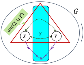
Figure 7: Search space for finding a restricted minimal separating set $Z$ for $X$ and $Y$ in an AMP chain graph $G$, when a set of nodes $S$ not containing $X$ and $Y$ is given.

Informally, search space of finding a restricted minimal separating set $Z$ for $X$ and $Y$ in an AMP chain graph $G$, when a set of nodes $S$ not containing $X$ and $Y$ is given, is limited to $ant(X\cup Y)$, as shown in Figure 7. Therefore, Problem 3 is solved by testing if $S^{\prime}=S\cap ant(X\cup Y)$ separates $X$ and $Y$.

Input: A set $S$ of nodes not containing $X$ and $Y$ in the AMP chain graph $G$.

Output: If there is a subset of $S$ that separates $X$ from $Y$ then the algorithm returns $Z\subseteq S$ that separates $X$ from $Y$ otherwise, returns FALSE.

/* Building the search space according to Theorem 9. */

1 Construct $G_{ant(X\cup Y)}$;

2 Construct $(G_{ant(X\cup Y)})^{a}$;

3 Set $S^{\prime}=S\cap ant(X\cup Y)$;

4 Remove $S^{\prime}$ from $(G_{ant(X\cup Y)})^{a}$;

/* Using BFS algorithm to test the separability of the candidate set $S^{\prime}$. */

5 Starting from $X$, run BFS;

6 if $Y$ is met then

7      return FALSE

8else

9      return $Z=S^{\prime}$

10 end if

Algorithm 3 Restricted separation (Problem 3)

Analysis of Algorithm 3: This requires $O(|E_{H}^{a}|)$ time.

According to Theorem 9, Problem 4 is solved using Algorithm 3 and then, if False not returned, Algorithm 2 with $Z^{\prime}=S\cap ant(X\cup Y)$. The time complexity of this algorithm is also $O(|E_{H}^{a}|)$.

In order to solve Problem 5, i.e., to find the minimal set separating two disjoint non-adjacent subsets of nodes $X$ and $Y$ (instead of two single nodes) in an AMP chain graph $G$, first we build the undirected graph $(G_{ant(X\cup Y)})^{a}$. Next, starting out from this graph, we construct a new undirected graph $Aug(G:\alpha_{X},\alpha_{Y})$ by adding two artificial (dummy) nodes $\alpha_{X},\alpha_{Y}$, and connect them to those nodes that are adjacent to some node in $X$ and $Y$, respectively. So, the separation of $X$ and $Y$ in $(G_{ant(X\cup Y)})^{a}$ is equivalent to the separation of $\alpha_{X}$ and $\alpha_{Y}$ in $Aug(G:\alpha_{X},\alpha_{Y})$. Moreover, the minimal separating set for $\alpha_{X}$ and $\alpha_{Y}$ in $Aug(G:\alpha_{X},\alpha_{Y})$ cannot contain nodes from $(X\cup Y)$. Therefore, in order to find the minimal separating set for $X$ and $Y$ in $G$, it is suffice to find the minimal separating set for $\alpha_{X}$ and $\alpha_{Y}$ in $Aug(G:\alpha_{X},\alpha_{Y})$. So, we have reduced this problem to one of separation for single nodes, which can be solved using Algorithm 2.

Shen and Liang in (Shen and Liang, 1997) presents an efficient algorithm for enumerating all minimal $(X,Y)$-separators, separating given non-adjacent vertices $X$ and $Y$ in an undirected connected simple graph $G=(V,E)$. This algorithm requires $O(n^{3}R_{XY})$ time, where $|V|=n$ and $R_{XY}$ is the number of minimal $(X,Y)$-separators. The algorithm can be generalized for enumerating all minimal $(X,Y)$-separators that separate non-adjacent vertex sets $X,Y\subseteq V$, and it requires $O(n^{2}(n-n_{X}-n_{Y})R_{XY})$ time. In this case, $|X|=n_{X}$, $|Y|=n_{Y}$, and $R_{XY}$ is the number of all minimal $(X,Y)$-separators. According to Theorem 6, using this algorithm for $(G_{ant(X\cup Y)})^{a}$ solves Problem 6.

Remark 10

Since DAGs (directed acyclic graphs) are subclass of AMP chain graphs, one can use the same technique to enumerate all minimal separators in DAGs.

4 PC-like Algorithm

In this section we explain the original PC-like algorithm proposed in (Peña, 2012) briefly, and we show that this version of the PC-like algorithm is order-dependent, in the sense that the output can depend on the order in which the variables are given. We propose modifications of the PC-like algorithm that remove (part or all of) this order-dependence.

4.1 Order-Dependent PC-like algorithm

The PC-like algorithm for learning AMP CGs under the faithfulness assumption proposed in (Peña, 2012) is formally described in Algorithm 4 for the reader’s convenience.

Input: A set $V$ of nodes and a probability distribution $p$ faithful to an unknown AMP CG $G$ and an ordering order($V$) on the variables.

Output: A CG $H$ that is triplex equivalent to $G$.

1 Let $H$ denote the complete undirected graph over $V$;

/* Skeleton Recovery */

2 for $i\leftarrow 0$ to $|V_{H}|-2$ do

3       while possible do

             Select any ordered pair of nodes $u$ and $v$ in $H$ such that $u\in ad_{H}(v)$ and $|[ad_{H}(u)\cup ad_{H}(ad_{H}(u))]\setminus\{u,v\}|\geq i$, using order($V$); /* $ad_{H}(x):=\{y\in V|x\mathrel{\leavevmode\hbox to16.51pt{\vbox to5.2pt{\text{[drawing]}}}}y,y\mathrel{\leavevmode\hbox to14.63pt{\vbox to5.2pt{\text{[drawing]}}}}x,\textrm{ or }x\mathrel{\leavevmode\hbox to14.63pt{\vbox to0.4pt{\text{[drawing]}}}}y\}$ */

4             if there exists $S\subseteq([ad_{H}(u)\cup ad_{H}(ad_{H}(u))]\setminus\{u,v\})$ s.t. $|S|=i$ and $u\perp\!\!\!\perp_{p}v|S$ (i.e., $u$ is independent of $v$ given $S$ in the probability distribution $p$) then

5                   Set $S_{uv}=S_{vu}=S$;

6                   Remove the edge $u\mathrel{\leavevmode\hbox to14.63pt{\vbox to0.4pt{\text{[drawing]}}}}v$ from $H$;

7                  

8             end if

9            

10       end while

11      

12 end for

/* Orientation phase: */

13 while possible do

14       Apply rules R1-R4 in Figure 10 to $H$.

15 end while

16Replace every edge $\mathrel{\leavevmode\hbox to14.63pt{\vbox to4.6pt{\text{[drawing]}}}}$ ($\mathrel{\leavevmode\hbox to14.63pt{\vbox to4.6pt{\text{[drawing]}}}}$) in $H$ with $\mathrel{\leavevmode\hbox to14.63pt{\vbox to5.2pt{\text{[drawing]}}}}$ ($\mathrel{\leavevmode\hbox to14.63pt{\vbox to0.4pt{\text{[drawing]}}}}$);

return $H$.

Algorithm 4 The order-dependent PC-like algorithm for learning AMP chain graphs (Peña, 2012)

In applications we do not have perfect conditional independence information. Instead, we assume that we have an i.i.d. sample of size $n$ of $V=(X_{1},\dots,Xp)$. In the PC-like algorithm (Peña, 2012) all conditional independence queries are estimated by statistical conditional independence tests at some pre-specified significance level (p.value) $\alpha$. For example, if the distribution of $V$ is multivariate Gaussian, one can test for zero partial correlation, see, e.g., (Kalisch and Bühlmann, 2007). For this purpose, we used the $\mathsf{gaussCItest()}$ function from the R package pcalg throughout this paper. Let order($V$) denote an ordering on the variables in $V$. We now consider the role of order($V$) in every step of the algorithm.

In the skeleton recovery phase of the PC-like algorithm (Peña, 2012; Peña and Gómez-Olmedo, 2016) (lines 2-10 of Algorithm 4), the order of variables affects the estimation of the skeleton and the separating sets. In particular, at each level of $i$, the order of variables determines the order in which pairs of adjacent vertices and subsets $S$ of their adjacency sets are considered (see lines 4 and 5 in Algorithm 4). The skeleton $H$ is updated after each edge removal. Hence, the adjacency sets typically change within one level of $i$, and this affects which other conditional independencies are checked, since the algorithm only conditions on subsets of the adjacency sets. When we have perfect conditional independence information, all orderings on the variables lead to the same output. In the sample version, however, we typically make mistakes in keeping or removing edges. In such cases, the resulting changes in the adjacency sets can lead to different skeletons, as illustrated in Example 2.

Moreover, different variable orderings can lead to different separating sets in the skeleton recovery phase. When we have perfect conditional independence information, this is not important, because any valid separating set leads to the correct triplex decision in the orientation phase. In the sample version, however, different separating sets in the skeleton recovery phase of the algorithm may yield different decisions about triplexes in the orientation phase (lines 12-15 of Algorithm 4). This is illustrated in Example 3. The examples were encountered when testing the PC-like algorithm by generating synthesized samples from the DAGs in Figure 8(a) and 9(a).

Example 2 (Order-dependent skeleton of the PC-like algorithm.)

Suppose that the distribution of $V=\{a,b,c,d,e\}$ is faithful to the DAG in Figure 8(a). This DAG encodes the following conditional independencies with minimal separating sets: $b\perp\!\!\!\perp c|a$ and $a\perp\!\!\!\perp e|\{b,c,d\}$.

Suppose that we have an i.i.d. sample of $(a,b,c,d,e)$, and that the following conditional independencies with minimal separating sets are judged to hold at some significance level $\alpha$: $b\perp\!\!\!\perp c|a$, $a\perp\!\!\!\perp e|d$,$a\perp\!\!\!\perp b|d$, $a\perp\!\!\!\perp c|d$, $b\perp\!\!\!\perp d|e$, and $c\perp\!\!\!\perp d|e$. Thus, the first conditional independence relation is correct, while the rest of them are false.

We now apply the skeleton recovery phase of the PC-like algorithm with two different orderings: $\textrm{order}_{1}(V)=(d,c,b,a,e)$ and $\textrm{order}_{2}(V)=(d,e,a,c,b)$. The resulting skeletons are shown in Figures 8(b) and 8(c), respectively.

Figure 8: Order-dependent skeleton of the PC-like algorithm. (a) The DAG $G$, (b) the skeleton returned by Algorithm 4 with $\textrm{order}_{1}(V)$, (c) the skeleton returned by Algorithm 4 with $\textrm{order}_{2}(V)$.

We see that the skeletons are different, and that both are incorrect as the edges $a\mathrel{\leavevmode\hbox to14.63pt{\vbox to0.4pt{\text{[drawing]}}}}b,a\mathrel{\leavevmode\hbox to14.63pt{\vbox to0.4pt{\text{[drawing]}}}}c,b\mathrel{\leavevmode\hbox to14.63pt{\vbox to0.4pt{\text{[drawing]}}}}d,$ and $c\mathrel{\leavevmode\hbox to14.63pt{\vbox to0.4pt{\text{[drawing]}}}}d$ are missing. The skeleton for $\textrm{order}_{2}(V)$ contains an additional error, as there is an additional edge $b\mathrel{\leavevmode\hbox to14.63pt{\vbox to0.4pt{\text{[drawing]}}}}c$. We now go through Algorithm 4 to see what happened. We start with a complete undirected graph on $V$. When $i=0$, variables are tested for marginal independence, and the algorithm correctly does not remove any edge. When $i=1$, there are six pairs of vertices that are thought to be conditionally independent given a subset of size one. Table 1 shows the trace table of Algorithm 4 for $i=1$ and $\textrm{order}_{1}(V)=(d,c,b,a,e)$.

Table 1: The trace table of Algorithm 4 for $i=1$ and $\textrm{order}_{1}(V)=(d,c,b,a,e)$. For simplicity, we define $ADJ_{H}(u):=[ad_{H}(u)\cup ad_{H}(ad_{H}(u))]\setminus\{u,v\}$.

Ordered Pair $(u,v)$	$ADJ_{H}(u)$	$S_{uv}$	Is $S_{uv}\subseteq ADJ_{H}(u)$?	Is $u\mathrel{\leavevmode\hbox to14.63pt{\vbox to0.4pt{\text{[drawing]}}}}v$ removed?
$(d,c)$	$\{a,b,e\}$	$\{e\}$	Yes	Yes
$(d,b)$	$\{a,c,e\}$	$\{e\}$	Yes	Yes
$(c,b)$	$\{a,d,e\}$	$\{a\}$	Yes	Yes
$(c,a)$	$\{b,d,e\}$	$\{d\}$	Yes	Yes
$(b,a)$	$\{c,d,e\}$	$\{d\}$	Yes	Yes
$(a,e)$	$\{d\}$	$\{d\}$	Yes	Yes

Table 2 shows the trace table of Algorithm 4 for $i=1$ and $\textrm{order}_{2}(V)=(d,e,a,c,b)$.

Table 2: The trace table of Algorithm 4 for $i=1$ and $\textrm{order}_{2}(V)=(d,e,a,c,b)$. For simplicity, we define $ADJ_{H}(u):=[ad_{H}(u)\cup ad_{H}(ad_{H}(u))]\setminus\{u,v\}$.

Ordered Pair $(u,v)$	$ADJ_{H}(u)$	$S_{uv}$	Is $S_{uv}\subseteq ADJ_{H}(u)$?	Is $u\mathrel{\leavevmode\hbox to14.63pt{\vbox to0.4pt{\text{[drawing]}}}}v$ removed?
$(d,c)$	$\{a,b,e\}$	$\{e\}$	Yes	Yes
$(d,b)$	$\{a,c,e\}$	$\{e\}$	Yes	Yes
$(e,a)$	$\{b,c,d\}$	$\{d\}$	Yes	Yes
$(a,c)$	$\{b,d,e\}$	$\{d\}$	Yes	Yes
$(a,b)$	$\{d,e\}$	$\{d\}$	Yes	Yes
$(c,b)$	$\{d,e\}$	$\{a\}$	No	No
$(b,c)$	$\{c,e\}$	$\{a\}$	No	No

No conditional independency is found when $i=2.$

Example 3 (Order-dependent separators & triplexes of the PC-like algorithm.)

Suppose that the distribution of $V=\{a,b,c,d,e\}$ is faithful to the DAG in Figure 9(a). This DAG encodes the following conditional independencies with minimal separating sets: $a\perp\!\!\!\perp d|b,a\perp\!\!\!\perp e|\{b,c\},a\perp\!\!\!\perp e|\{c,d\},b\perp\!\!\!\perp c,b\perp\!\!\!\perp e|d,$ and $c\perp\!\!\!\perp d$.

Suppose that we have an i.i.d. sample of $(a,b,c,d,e)$. Assume that all true conditional independencies are judged to hold except $c\perp\!\!\!\perp d$. Suppose that $c\perp\!\!\!\perp d|b$ and $c\perp\!\!\!\perp d|e$ are thought to hold. Thus, the first is correct, while the second is false. We now apply the orientation phase of the PC-like algorithm with two different orderings: $\textrm{order}_{1}(V)=(d,c,b,a,e)$ and $\textrm{order}_{3}(V)=(c,d,e,a,b)$. The resulting CGs are shown in Figures 9(b) and 9(c), respectively. Note that while the separating set for vertices $c$ and $d$ with $\textrm{order}_{1}(V)$ is $S_{dc}=S_{cd}=\{b\}$, the separating set for them with $\textrm{order}_{2}(V)$ is $S_{cd}=S_{dc}=\{e\}$.

Figure 9: Order-dependent separators and triplexes of the PC-like algorithm. (a) The DAG $G$, (b) the CG returned by Algorithm 4 with $\textrm{order}_{1}(V)$, (c) the CG returned by Algorithm 4 with $\textrm{order}_{3}(V)$.

This illustrates that order-dependent separating sets in the skeleton recovery phase of the sample version of the PC-algorithm can lead to order-dependent triplexes in the orientation phase of the algorithm.

4.2 Order-Independent ( Stable-) PC-like Algorithm

As shown in the previous section, the original PC-like algorithm is order-dependent. In this section we propose modifications of the PC-like algorithm, i.e., the Stable PC-like for AMP chain graphs (Stable-PC4AMP), Conservative PC-like for AMP CGs (Conservative-PC4AMP), and Stable-Conservative-PC4AMP for learning the structure of AMP chain graphs under the faithfulness assumption that remove part or all of the order-dependence. The order-dependence can become very problematic for high-dimensional data, leading to highly variable results and conclusions for different variable orderings. The second limitation of the PC-like algorithm is that the runtime of the algorithm, in the worst case, is exponential to the number of variables, and thus it is inefficient when applying to high dimensional datasets such as gene expression. We now propose several modifications of the original PC-like algorithm for learning AMP chain graphs (and hence also of the related algorithms), called stable PC-like, that remove the order-dependence in the various stages of the algorithm, analogously to what (Colombo and Maathuis, 2014) did for the original PC algorithm in the case of DAGs. The stable PC-like algorithm for AMP chain graphs can be used to parallelize the conditional independence (CI) tests at each level of the skeleton recovery algorithm. So, the CI tests at each level can be grouped and distributed over different cores of the computer, and the results can be integrated at the end of each level. Consequently, the runtime of our parallelized stable PC-like algorithm is much shorter than the original PC-like algorithm for learning AMP chain graphs. Furthermore, this approach enjoys the advantage of knowing the number of CI tests of each level in advance. This allows the CI tests to be evenly distributed over different cores, so that the parallelized algorithm can achieve maximum possible speedup. In order to explain the details of the stable PC-like algorithm for AMP chain graphs, we discuss the skeleton and the orientation rules, respectively.

We first consider estimation of the skeleton in the adjacency search (skeleton recovery phase) of the PC-like algorithm for AMP chain graphs (lines 2-10 of Algorithm 4). The pseudocode for our modification is given in Algorithm 5 (lines 2-13). The resulting PC-like algorithm for learning AMP chain graphs in Algorithm 5 is called Stable PC-like for AMP CGs (Stable-PC4AMP).

Input: A set $V$ of nodes and a probability distribution $p$ faithful to an unknown AMP CG $G$ and an ordering order($V$) on the variables.

Output: A CG $H$ that is triplex equivalent to $G$.

1 Let $H$ denote the complete undirected graph over $V=\{v_{1},\dots,v_{n}\}$;

/* Skeleton Recovery: */

2 for $i\leftarrow 0$ to $|V_{H}|-2$ do

3       for $j\leftarrow 1$ to $|V_{H}|$ do

4             Set $a_{H}(v_{j})=ad_{H}(v_{j})\cup ad_{H}(ad_{H}(v_{j}))$;

             /* $ad_{H}(x):=\{y\in V|x\mathrel{\leavevmode\hbox to14.63pt{\vbox to5.2pt{\text{[drawing]}}}}y,y\mathrel{\leavevmode\hbox to14.63pt{\vbox to5.2pt{\text{[drawing]}}}}x,\textrm{ or }x\mathrel{\leavevmode\hbox to14.63pt{\vbox to0.4pt{\text{[drawing]}}}}y\}$ */

5            

6       end for

7      while possible do

8             Select any ordered pair of nodes $u$ and $v$ in $H$ such that $u\in ad_{H}(v)$ and $|a_{H}(u)\setminus\{u,v\}|\geq i$, using order($V$);

9            if there exists $S\subseteq(a_{H}(u)\setminus\{u,v\})$ s.t. $|S|=i$ and $u\perp\!\!\!\perp_{p}v|S$ (i.e., $u$ is independent of $v$ given $S$ in the probability distribution $p$) then

10                   Set $S_{uv}=S_{vu}=S$;

11                   Remove the edge $u\mathrel{\leavevmode\hbox to14.63pt{\vbox to0.4pt{\text{[drawing]}}}}v$ from $H$;

12                  

13             end if

14            

15       end while

16      

17 end for

/* Orientation phase: */

18 while possible do

19       Apply rules R1-R4 in Figure 10 to $H$.

20 end while

21Replace every edge $\mathrel{\leavevmode\hbox to14.63pt{\vbox to4.6pt{\text{[drawing]}}}}$ ($\mathrel{\leavevmode\hbox to14.63pt{\vbox to4.6pt{\text{[drawing]}}}}$) in $H$ with $\mathrel{\leavevmode\hbox to14.63pt{\vbox to5.2pt{\text{[drawing]}}}}$ ($\mathrel{\leavevmode\hbox to14.63pt{\vbox to0.4pt{\text{[drawing]}}}}$);

return $H$.

Algorithm 5 The order-independent ( Stable-) PC-like algorithm for learning AMP CGs (Stable-PC4AMP)

Figure 10: Orientation rules in Algorithms 4 and 5: Rules R1-R4 (Peña, 2012)

The main difference between Algorithms 4 and 5 is given by the for-loop on lines 3-5 in the latter one, which computes and stores the adjacency sets $a_{H}(v_{i})$ of all variables after each new size $i$ of the conditioning sets. These stored adjacency sets $a_{H}(v_{i})$ are used whenever we search for conditioning sets of this given size $i$. Consequently, an edge deletion on line 10 no longer affects which conditional independencies are checked for other pairs of variables at this level of $i$.

In other words, at each level of $i$, Algorithm 5 records which edges should be removed, but for the purpose of the adjacency sets it removes these edges only when it goes to the next value of $i$. Besides resolving the order-dependence in the estimation of the skeleton, our algorithm has the advantage that it is easily parallelizable at each level of $i$ i.e., computations required for $i$-level can be performed in parallel. The Stable-PC4AMP algorithm is correct, i.e. it returns an AMP CG the given probability distribution is faithful to (Theorem 11), and yields order-independent skeletons in the sample version (Theorem 12). We illustrate the algorithm in Example 4.

Theorem 11

Let the distribution of $V$ be faithful to an AMP CG $G$, and assume that we are given perfect conditional independence information about all pairs of variables $(u,v)$ in $V$ given subsets $S\subseteq V\setminus\{u,v\}$. Then the output of the Stable-PC4AMP algorithm is an AMP CG that is Markov equivalent with $G$.

Proof  The proof of Theorem 11 is completely analogous to the proof of Theorem 1 for the original PC-like algorithm in (Peña, 2012).  

Theorem 12

The skeleton resulting from the sample version of the Stable-PC4AMP algorithm for AMP CGs is order-independent.

Proof  We consider the removal or retention of an arbitrary edge $u\mathrel{\leavevmode\hbox to14.63pt{\vbox to0.4pt{\text{[drawing]}}}}v$ at some level $i$. The ordering of the variables determines the order in which the edges (line 7 of Algorithm 5) and the subsets $S$ of $a_{H}(u)$ and $a_{H}(v)$ (line 8 of Algorithm 5) are considered. By construction, however, the order in which edges are considered does not affect the sets $a_{H}(u)$ and $a_{H}(v)$.

If there is at least one subset $S$ of $a_{H}(u)$ or $a_{H}(v)$ such that $u\perp\!\!\!\perp_{p}v|S$, then any ordering of the variables will find a separating set for $u$ and $v$ (but different orderings may lead to different separating sets as illustrated in Example 3). Conversely, if there is no subset $S^{\prime}$ of $a_{H}(u)$ or $a_{H}(v)$ such that $u\perp\!\!\!\perp_{p}v|S^{\prime}$, then no ordering will find a separating set.

Hence, any ordering of the variables leads to the same edge deletions, and therefore to the same skeleton.  

Example 4 (Order-independent skeletons)

We go back to Example 2, and consider the sample version of Algorithm 5. The algorithm now outputs the skeleton shown in Figure 8(b) for both orderings $\textrm{order}_{1}(V)$ and $\textrm{order}_{2}(V)$.

We again go through the algorithm step by step. We start with a complete undirected graph on $V$. No conditional independence found when $i=0$. When $i=1$, the algorithm first computes the new adjacency sets: $a_{H}(v)=V\setminus\{v\},\forall v\in V$. There are six pairs of variables that are thought to be conditionally independent given a subset of size 1 (see Table 3). Since the sets $a_{H}(v)$ are not updated after edge removals, it does not matter in which order we consider the ordered pairs. Any ordering leads to the removal of six edges.

Table 3: The trace table of Algorithm 5 for $i=1$, $\textrm{order}_{1}(V)=(d,c,b,a,e)$, and $\textrm{order}_{2}(V)=(d,e,a,c,b)$. For simplicity, we define $ADJ_{H}(u):=[ad_{H}(u)\cup ad_{H}(ad_{H}(u))]\setminus\{u,v\}$.

Ordered Pair $(u,v)$	$ADJ_{H}(u)$	$S_{uv}$	Is $S_{uv}\subseteq ADJ_{H}(u)$?	Is $u\mathrel{\leavevmode\hbox to14.63pt{\vbox to0.4pt{\text{[drawing]}}}}v$ removed?
$(d,c)$	$\{a,b,e\}$	$\{e\}$	Yes	Yes
$(d,b)$	$\{a,c,e\}$	$\{e\}$	Yes	Yes
$(c,b)$	$\{a,d,e\}$	$\{a\}$	Yes	Yes
$(c,a)$	$\{b,d,e\}$	$\{d\}$	Yes	Yes
$(b,a)$	$\{c,d,e\}$	$\{d\}$	Yes	Yes
$(a,e)$	$\{b,c,d\}$	$\{d\}$	Yes	Yes

Now, we propose a method to resolve the order-dependence in the determination of the triplexes in AMP chain graphs, by extending the approach in (Ramsey et al., 2006) for unshielded colliders recovery in DAGs.

Our proposed Conservative PC-like algorithm for AMP CGs (Conservative-PC4AMP) works as follows. Let $H$ be the undirected graph resulting from the skeleton recovery phase of the PC-like algorithm (Algorithm 4). For all unshielded triples $(X_{i},X_{j},X_{k})$ in $H$, determine all subsets $S$ of $ad_{H}(X_{i})\cup ad_{H}(ad_{H}(X_{i}))$ and of $ad_{H}(X_{k})\cup ad_{H}(ad_{H}(X_{k}))$ that make $X_{i}$ and $X_{k}$ conditionally independent, i.e., that satisfy $X_{i}\perp\!\!\!\perp_{p}X_{k}|S$. We refer to such sets as separating sets. The triple $(X_{i},X_{j},X_{k})$ is labelled as unambiguous if at least one such separating set is found and either $X_{j}$ is in all separating sets or in none of them; otherwise it is labelled as ambiguous. If the triple is unambiguous, it is labeled and then oriented as described in Algorithm 4. So, the orientation rules are adapted so that only unambiguous triples are oriented.

We refer to the combination of the Stable-PC4AMP and Conservative-PC4AMP algorithms for AMP chain graphs as the Stable-Conservative-PC4AMP algorithm.

Theorem 13

Let the distribution of $V$ be faithful to an AMP CG $G$, and assume that we are given perfect conditional independence information about all pairs of variables $(u,v)$ in $V$ given subsets $S\subseteq V\setminus\{u,v\}$. Then the output of the Conservative-PC4AMP / Stable-Conservative-PC4AMP algorithm is an AMP CG that is Markov equivalent with $G$.

Proof  The skeleton of the learned CG is correct by Theorem 11. Now, we prove that for any unshielded triple $(X_{i},X_{j},X_{k})$ in an AMP CG $G$, $X_{j}$ is either in all sets that p-separate $X_{i}$ and $X_{k}$ or in none of them. Since $X_{i},X_{k}$ are not adjacent, they are p-separated given some subset $S\setminus\{X_{i},X_{k}\}$ (see Algorithm 2). Based on the pathwise p-separation criterion for AMP CGs (see Definition 2), $X_{j}$ is a triplex node in $G$ if and only if $X_{j}\not\in An(S).$ So, $X_{j}\not\in S.$ On the other hand, if $X_{j}$ is a non-triplex node then $X_{j}\in S$, for all $S$ that p-separate $X_{i}$ and $X_{k}$. Because in this case, $X_{j}\in Co(An(X_{i}\cup X_{k}\cup S))$ and so there is an undirected path $X_{i}\mathrel{\leavevmode\hbox to14.63pt{\vbox to0.4pt{\text{[drawing]}}}}X_{j}\mathrel{\leavevmode\hbox to14.63pt{\vbox to0.4pt{\text{[drawing]}}}}X_{k}$ in $(G[X_{i}\cup X_{k}\cup S])^{a}$. Any set $S\setminus\{X_{i},X_{k}\}$ that does not contain $X_{j}$ will fail to p-separate $X_{i}$ and $X_{k}$ because of this undirected path. As a result, unshielded triples are all unambiguous. Since all unshielded triples are unambiguous, the orientation rules are as in the original ( Stable-) PC-like algorithm. Therefore, the output of the Conservative-PC4AMP/Stable-Conservative-PC4AMP algorithm is an AMP CG that is Markov equivalent with $G$.  

Theorem 14

The decisions about triplexes in the sample version of the algorithm for AMP chain graphs recovery by Stable-Conservative-PC4AMP is order-independent.

Proof  The Stable-Conservative-PC4AMP algorithm have order-independent skeleton, by Theorem 12. In particular, this means that their unshielded triples and adjacency sets are order-independent. The decision about whether an unshielded triple is unambiguous and/or a triplex is based on the adjacency sets of nodes in the triple, which are order independent.  

Example 5 (Order-independent decisions about triplexes)

We consider the sample versions of the Stable-Conservative-PC4AMP algorithm for AMP chain graphs, using the same input as in Example 3. In particular, we assume that all conditional independencies induced by the AMP CG in Figure 9(a) are judged to hold except $c\perp\!\!\!\perp d$. Suppose that $c\perp\!\!\!\perp d|b$ and $c\perp\!\!\!\perp d|e$ are thought to hold.

Denote the skeleton after the skeleton recovery phase by $H$. We consider the unshielded triple $(c,e,d)$. First, we compute $a_{H}(c)=\{a,b,d,e\}$ and $a_{H}(d)=\{a,b,c,e\}$. We now consider all subsets $S$ of these adjacency sets, and check whether $c\perp\!\!\!\perp d|S$. The following separating sets are found: $\{b\},\{e\}$, and $\{b,e\}$. Since $e$ is in some but not all of these separating sets, the Stable-Conservative-PC4AMP algorithm for AMP chain graphs determines that the triple is ambiguous, and no orientations are performed. The output of the algorithm is given in Figure 9(c).

At this point it should be clear why the modified PC-like algorithm for AMP chain graphs is labeled “conservative”: it is more cautious than the ( Stable-) PC-like algorithm for AMP chain graphs in drawing unambiguous conclusions about orientations. As we showed in Example 5, the output of the algorithm for AMP chain graphs recovery by Conservative-PC4AMP or Stable-Conservative-PC4AMP may not be triplex equivalent with the true AMP CG $G$, if the resulting CG contains an ambiguous triple.

Table 4 summarizes all order-dependence issues explained above and the corresponding modifications of the PC-like algorithm for AMP chain graphs that removes the given order-dependence problem.

Table 4: Order-dependence issues and corresponding modifications of the PC-like algorithm that remove the problem. “Yes” indicates that the corresponding aspect of the graph is estimated order-independently in the sample version.

	skeleton	triplexes decisions
PC-like algorithm for AMP CGs	No	No
Stable-PC4AMP	Yes	No
Stable-Conservative-PC4AMP	Yes	Yes

5 LCD-AMP Algorithm: Structure Learning by Decomposition

In this section, first, we address the issue of how to construct a $p$-separation tree from observed data, which is the heart of our decomposition-based algorithm. Then, we present an algorithm, called LCD-AMP, that shows how separation trees can be used to facilitate the decomposition of the structure learning of AMP chain graphs. The theoretical results are presented first, followed by descriptions of our algorithm that is the summary of the key results in our paper.

5.1 Constructing a p-Separation Tree from Observed Data

As proposed in (Xie et al., 2006), one can construct a $d$-separation tree from observed data. In this section we extend Theorem 2 of (Xie et al., 2006), and thereby prove that their method for constructing a separation tree from data is valid for AMP chain graphs. To construct an undirected independence graph in which the absence of an edge $u\mathrel{\leavevmode\hbox to14.63pt{\vbox to0.4pt{\text{[drawing]}}}}v$ implies $u\perp\!\!\!\perp v|V\setminus\{u,v\}$, we can start with a complete undirected graph, and then for each pair of variables $u$ and $v$, an undirected edge $u\mathrel{\leavevmode\hbox to14.63pt{\vbox to0.4pt{\text{[drawing]}}}}v$ is removed if $u$ and $v$ are independent conditional on the set of all other variables (Xie et al., 2006). For normally distributed data, the undirected independence graph can be efficiently constructed by removing an edge $u\mathrel{\leavevmode\hbox to14.63pt{\vbox to0.4pt{\text{[drawing]}}}}v$ if and only if the corresponding entry in the concentration matrix (inverse covariance matrix) is zero (Lauritzen, 1996, Proposition 5.2). For this purpose, performing a conditional independence test for each pair of random variables using the partial correlation coefficient can be used. If the $p$-value of the test is smaller than the given threshold, then there will be an edge on the output graph. For discrete data, a test of conditional independence given a large number of discrete variables may be of extremely low power. To cope with such difficulty, there are two fundamental ways to perform structure learning: (1) Parameter estimation techniques (Banerjee et al., 2008; Ravikumar et al., 2010) that utilize a factorization of the distribution according to the cliques of the graph to learn the underlying graph. These techniques assume a certain form of the potential function, and thereby relate the structure learning problem to one of finding a sparse maximum likelihood estimator of a distribution from its samples. (2) Algorithms based on learning conditional independence relations between the variables (Chow and Liu, 1968; Bresler et al., 2008; Netrapalli et al., 2010; Anandkumar et al., 2012) that they do not need knowledge of the underlying parametrization to learn the graph. These methods are based on comparing all possible neighborhoods of a node to find one which has the maximum influence on the node. In (Edwards, 2000, Chapter 6), (Bromberg et al., 2009), and (de Abreu et al., 2010b) there are other methods for UIG learning, including some for data with both continuous and discrete variables. All these methods can be used to construct separation trees from data.

Theorem 15

A junction tree constructed from an undirected independence graph for AMP CG $G$ is a $p$-separation tree for $G$.

Proof  See Appendix A.  

A $p$-separation tree $T$ only requires that all $p$-separation properties of $T$ also hold for AMP CG $G$, but the reverse is not required. Thus we only need to construct an undirected independence graph that may have fewer conditional independencies than the augmented graph, and this means that the undirected independence graph may have extra edges added to the augmented graph. As (Xie et al., 2006) observe for $d$-separation in DAGs, if all nodes of a $p$-separation tree contain only a few variables, “the null hypothesis of the absence of an undirected edge may be tested statistically at a larger significance level.”

Since there are standard algorithms for constructing junction trees from UIGs (Cowell et al., 1999, Chapter 4, Section 4), the construction of separation trees reduces to the construction of UIGs. In this sense, Theorem 15 enables us to exploit various techniques for learning UIGs to serve our purpose. More suggested methods for learning UIGs from data, in addition to the above mentioned techniques, can be found in (Ma et al., 2008).

Example 6

To construct a $p$-separation tree for the AMP CG $G$ in Figure 4(a), at first an undirected independence graph is constructed by starting with a complete graph and removing an edge $u\mathrel{\leavevmode\hbox to14.63pt{\vbox to0.4pt{\text{[drawing]}}}}v$ if $u\perp\!\!\!\perp v|V\setminus\{u,v\}$. An undirected graph obtained in this way is the augmented graph of AMP CG $G$. In fact, we only need to construct an undirected independence graph which may have extra edges added to the augmented graph. Next triangulate the undirected graph and finally obtain the $p$-separation tree, as shown in Figure 4(c) and Figure 5 respectively.

5.2 The LCD-AMP Algorithm for Learning AMP Chain Graphs

By applying the following theorem to structural learning, we can split a problem of searching for $p$-separators and building the skeleton of a CG into small problems for every node of $p$-separation tree $T$.

Theorem 16

Let $T$ be a $p$-separation tree for AMP CG $G$ and $u$ and $v$ be two vertices that do not belong to the same chain component. So, vertices $u$ and $v$ are $p$-separated by $S\subseteq V$ in $G$ if and only if (i) $u$ and $v$ are not contained together in any node $C$ of $T$ or (ii) there exists a node $C$ that contains both $u$ and $v$ such that a subset $S^{\prime}$ of $C$ $p$-separates $u$ and $v$.

Proof  See Appendix A.  

According to Theorem 16, a problem of searching for a $p$-separator $S$ of $u$ and $v$ in all possible subsets of $V$ is localized to all possible subsets of nodes in a $p$-separation tree that contain $u$ and $v$. For a given $p$-separation tree $T$ with the node set $C=\{C_{1},\dots,C_{H}\}$, we can recover the skeleton and all triplexes for an AMP CG using a constraint-based algorithm, called LCD-AMP, that contains two main steps: (a) determining the skeleton by a divide-and-conquer approach; (b) determining triplexes and orienting some of the undirected edges into directed edges according to a set of rules applied iteratively with localized search for $p$-separators. We elaborate on each phase of this algorithm below.

LCD-AMP Description: (a) Skeleton Recovery. This phase has two steps. First, we construct a local skeleton for every node $C_{h}$ of $T$, which is constructed by starting with a complete undirected subgraph and removing an undirected edge $u\mathrel{\leavevmode\hbox to14.63pt{\vbox to0.4pt{\text{[drawing]}}}}v$ if there is a subset $S$ of $C_{h}$ such that $u$ and $v$ are independent conditional on $S$. For this purpose, we can use the PC-like algorithm Peña (2012) or the Stable-PC4AMP algorithm (Algorithm 5, line 2-13) in Algorithm 6 (line 3-11). Second, in order to construct the global skeleton (line 13-23 of Algorithm 6), we combine all these local skeletons together. Note that it is possible that some edges that are present in some local skeletons may be absent in other local skeletons. Also, two non-adjacent vertices $u$ and $v$ in the AMP CG $G$ that belong to the same chain component may be adjacent in the temporary global skeleton. (Note that Theorem 16 only guarantees the existence of the $p$-separators for those non-adjacent vertices that do not belong to the same chain component. In Appendix A, we provide an example that shows that Theorem 16 cannot be strengthened.) In order to remove the extra edges in the resulting undirected graph, we apply a removal procedure that is similar to the skeleton recovery phase of the PC-like algorithm. However, instead of the complete undirected graph we use the resulting undirected graph obtained in the previous step. (b) Orientation phase. In this phase (line 25-28 of Algorithm 6), we orient undirected edges using rules R1-R4 in (Peña, 2012; Peña and Gómez-Olmedo, 2016) (illustrated in Figure 10 for the reader’s convenience). The whole process is formally described in Algorithm 6.

Input: A probability distribution $p$ faithful to an unknown AMP CG $G$.

Output: A chain graph $H$ that is triplex equivalent to the AMP CG $G$.

1 Construct a $p$-separation tree $T$ with a node set $C=\{C_{1},\dots,C_{I}\}$ as discussed in Section 5.1;

2 Set $S=\emptyset$;

/* Local skeleton recovery: */

3 for $i\leftarrow 1$ to $I$ do

4       Start from a complete undirected graph $\bar{G}_{i}$ with vertex set $C_{i}$;

5       for each vertex pair $\{u,v\}\subseteq C_{i}$  do

6            if $\exists S_{uv}\subseteq C_{i}\textrm{ such that }u\perp\!\!\!\perp v|S_{uv}$ then

7                   Delete the edge $u\mathrel{\leavevmode\hbox to14.63pt{\vbox to0.4pt{\text{[drawing]}}}}v$ in $\bar{G}_{i}$;

8                   Add $S_{uv}$ to $S$;

9             end if

10            

11       end for

12      

13 end for

/* Global skeleton recovery: */

14 Initialize the edge set $\bar{E}_{V}$ of $\bar{G}_{V}$ as the union of all edge sets of $\bar{G}_{i},i=1,\dots,I$;

15 Set $H=\bar{G}_{V}$;

16 for $i\leftarrow 0$ to $|V_{H}|-2$ do

17       while possible do

             Select any ordered pair of nodes $u$ and $v$ in $H$ such that $u\in ad_{H}(v)$ and $|[ad_{H}(u)\cup ad_{H}(ad_{H}(u))]\setminus\{u,v\}|\geq i$; /* $ad_{H}(x):=\{y\in V|x\mathrel{\leavevmode\hbox to14.63pt{\vbox to5.2pt{\text{[drawing]}}}}y,y\mathrel{\leavevmode\hbox to14.63pt{\vbox to5.2pt{\text{[drawing]}}}}x,\textrm{ or }x\mathrel{\leavevmode\hbox to14.63pt{\vbox to0.4pt{\text{[drawing]}}}}y\}$ */

18             if there exists $S\subseteq([ad_{H}(u)\cup ad_{H}(ad_{H}(u))]\setminus\{u,v\})$ s.t. $|S|=i$ and $u\perp\!\!\!\perp_{p}v|S$ (i.e., $u$ is independent of $v$ given $S$ in the probability distribution $p$) then

19                   Set $S_{uv}=S_{vu}=S$;

20                   Remove the edge $u\mathrel{\leavevmode\hbox to14.63pt{\vbox to0.4pt{\text{[drawing]}}}}v$ from $H$;

21                  

22             end if

23            

24       end while

25      

26 end for

/* Orientation phase (Peña, 2012): */

27 while possible do

28       Apply rules R1-R4 in Figure 10 to $H$.

      /* A block is represented by a perpendicular line at the edge end such as in $\mathrel{\leavevmode\hbox to14.63pt{\vbox to4.6pt{\text{[drawing]}}}}$ or $\mathrel{\leavevmode\hbox to14.63pt{\vbox to4.6pt{\text{[drawing]}}}}$, and it means that the edge cannot be a directed edge pointing in the direction of the block. Note that $\mathrel{\leavevmode\hbox to14.63pt{\vbox to4.6pt{\text{[drawing]}}}}$ means that the edge must be undirected. The ends of some of the edges in the rules are labeled with a circle such as in $\mathrel{\leavevmode\hbox to14.63pt{\vbox to4.32pt{\text{[drawing]}}}}$ or $\mathrel{\leavevmode\hbox to14.63pt{\vbox to0.4pt{\text{[drawing]}}}}$. The circle represents an unspecified end, i.e. a block or nothing. */

29      

30 end while

31Replace every edge $\mathrel{\leavevmode\hbox to14.63pt{\vbox to4.6pt{\text{[drawing]}}}}$ ($\mathrel{\leavevmode\hbox to14.63pt{\vbox to4.6pt{\text{[drawing]}}}}$) in $H$ with $\mathrel{\leavevmode\hbox to14.63pt{\vbox to5.2pt{\text{[drawing]}}}}$ ($\mathrel{\leavevmode\hbox to14.63pt{\vbox to0.4pt{\text{[drawing]}}}}$);

32 return $H$.

Algorithm 6 LCD-AMP : A decomposition-based recovery algorithm for AMP CGs

We prove that the global skeleton and all triplexes obtained by applying the decomposition in Algorithm 6 are correct, that is, they are the same as those obtained from the joint distribution of $V$. In other words, LCD-AMP  returns a chain graph that is a member of a class of triplex equivalent AMP chain graphs; see Appendix A for proof details. Note that separators in a $p$-separation tree may not be complete in the augmented graph. Thus the decomposition is weaker than the decomposition usually defined for parameter estimation (Cowell et al., 1999; Lauritzen, 1996).

Remark 17

One can apply Algorithm 3 in (Roverato and Rocca, 2006) to to the resulting chain graph of Algorithm 6 to obtain the largest deflagged graph. Also, one can apply Algorithm 1 in (Sonntag and Peña, 2015) to the resulting chain graph of Algorithm 6 to obtain the AMP essential graph.

5.3 Complexity Analysis of the LCD-AMP Algorithm

Here we start by comparing our algorithm with the main algorithm in (Xie et al., 2006) that is designed specifically for DAG structural learning when the underlying graph structure is a DAG. We make this choice of the DAG specific algorithm so that both algorithms can have the same separation tree as input and hence are directly comparable.

The same advantages mentioned by (Xie et al., 2006) for their BN structural learning algorithm hold for our algorithm when applied to AMP CGs. For the reader’s convenience, we list them here. First, by using the $p$-separation tree, independence tests are performed only conditionally on smaller sets contained in a node of the $p$-separation tree rather than on the full set of all other variables. Thus our algorithm has higher power for statistical tests. Second, the computational complexity can be reduced. The number of conditional independence tests for constructing the equivalence class is used as characteristic operation for this complexity analysis. Decomposition of graphs is a computationally simple task compared to the task of testing conditional independence for a large number of triples of sets of variables. The triangulation of an undirected graph is used in our algorithms to construct a $p$-separation tree from an undirected independence graph. Although the problem for optimally triangulating an undirected graph is NP-hard, sub-optimal triangulation methods (Berry et al., 2004) may be used provided that the obtained tree does not contain too large nodes to test conditional independencies. Two of the best known algorithms are lexicographic search and maximum cardinality search, and their complexities are $O(|V||E|)$ and $O(|V|+|E|)$, respectively (Berry et al., 2004). Thus in our algorithms, conditional independence tests dominate algorithmic complexity.

For the sake of complexity analysis, Algorithm 6 can be divided into four parts: (1) construction of the p-separation tree, (2) local skeleton recovery (lines 3–11), (3) global skeleton recovery (lines 12–22), and (4) orientation phase (lines 23-25). Part (1) includes the construction of the UIG, which takes at most $O(n^{2})$ conditional independence tests, where $n$ is the number of variables in the data set. Part (2) and (3) together require $O(Hm^{2}2^{m})$ as claimed in (Xie et al., 2006, Section 6), where $H$ is the number of $p$-separation tree nodes (usually $H\ll|V|$) and $m=\max_{h}|C_{h}|$ where $|C_{h}|$ denotes the number of variables in $C_{h}$ ($m$ usually is much less than $|V|$). Part (4) does not require any conditional independence tests.

6 Experimental Evaluation

In this section we evaluate the performance of our algorithms in various setups using simulated / synthetic data sets. We first compare the performance of our proposed algorithms, i.e., Stable-PC4AMP, Conservative-PC4AMP, Stable-Conservative-PC4AMP and LCD-AMP with the original PC-like  learning algorithms by running them on randomly generated AMP chain graphs. We then compare our algorithms, i.e., Stable-PC4AMP and LCD-AMP algorithms with the PC-like algorithm on different discrete Bayesian networks such as ASIA, INSURANCE, ALARM, and HAILFINDER that have been widely used in evaluating the performance of structural learning algorithms. Empirical simulations show that our algorithm achieves competitive results with the PC-like and Stable-PC4AMP learning algorithms; in particular, in the Gaussian case the decomposition-based algorithm outperforms the PC-like and Stable-PC4AMP algorithms. Algorithms 6 and the PC-like and Stable-PC4AMP algorithms have been implemented in the R language. All code, data, and the results reported here are based on our R implementation available at the following GitHub link https://github.com/majavid/AMPCGs2019. We do not consider the case of mixed continuous and discrete data in this paper, and leave this important and complex issue for future work; we only observe that this problem has been studied in the case of Markov networks and Bayesian networks, for example see (de Abreu et al., 2010a; Lauritzen and Jensen, 2001; Raghu et al., 2018; Andrews et al., 2018).

6.1 Performance Evaluation Metrics

We evaluate the performance of the proposed algorithms in terms of the six measurements that are commonly used by (Colombo and Maathuis, 2014; Ma et al., 2008; Tsamardinos et al., 2006) for constraint-based learning algorithms:

1. the true positive rate (TPR) is the ratio of the number of correctly identified edges over total number of edges (in true graph), i.e.,

   $$TPR=\frac{\textrm{true positive }(TP)}{\textrm{the number of real positive cases in the data }(Pos)},$$

2. the false positive rate (FPR) is the ratio of the number of incorrectly identified edges over total number of gaps, i.e.,

   $$FPR=\frac{\textrm{false positive }(FP)}{\textrm{the number of real negative cases in the data }(Neg)},$$

3. the true discovery rate (TDR) is the ratio of the number of correctly identified edges over total number of edges (both in estimated graph), i.e.,

   $$TDR=\frac{\textrm{true positive }(TP)}{\textrm{the total number of edges in the recovered CG}},$$

4. accuracy (ACC) is defined as

   $$ACC=\frac{\textrm{true positive }(TP)+\textrm{ true negative }(TN)}{Pos+Neg},$$

5. the structural Hamming distance (SHD) is the number of legitimate operations needed to change the current resulting graph to the true CG, where legitimate operations are: (i) add or delete an edge and (ii) insert, delete or reverse an edge orientation, and

6. run-time for the chain graph recovery algorithms.

Note that we use TPR, FPR, TDR, and ACC for comparing the skeletons of a learned structure and a ground truth graph. In principle, a large TDR, TPR and ACC, a small FPR and SHD indicate good performance.

To investigate the performance of the proposed learning methods in this paper, we use the same approach that Ma et al. (2008) used in evaluating the performance of the LCD algorithm on LWF chain graphs. We run our algorithms on randomly generated AMP chain graphs and then we compare the results and report summary error measures in all cases.

6.2 Performance Evaluation on Random AMP Chain Graphs (Gaussian case)

To investigate the performance of the proposed learning methods in this paper, we use the same approach that (Ma et al., 2008) used in evaluating the performance of the LCD algorithm on LWF chain graphs. We run our algorithms on randomly generated AMP chain graphs and then we compare the results and report summary error measures in all cases.

6.2.1 Data Generation Procedure

First we explain the way in which the random AMP chain graphs and random samples are generated. Given a vertex set $V$ , let $p=|V|$ and $N$ denote the average degree of edges (including undirected and pointing out and pointing in) for each vertex. We generate a random AMP chain graph on $V$ as follows:

• Order the $p$ vertices and initialize a $p\times p$ adjacency matrix $A$ with zeros;

• For each element in the lower triangle part of $A$, set it to be a random number generated from a Bernoulli distribution with probability of occurrence $s=N/(p-1)$;

• Symmetrize $A$ according to its lower triangle;

• Select an integer $k$ randomly from $\{1,\dots,p\}$ as the number of chain components;

• Split the interval $[1,p]$ into $k$ equal-length subintervals $I_{1},\dots,I_{k}$ so that the set of variables falling into each subinterval $I_{m}$ forms a chain component $C_{m}$;

• Set $A_{ij}=0$ for any $(i,j)$ pair such that $i\in I_{l},j\in I_{m}$ with $l>m$.

This procedure yields an adjacency matrix $A$ for a chain graph with $(A_{ij}=A_{ji}=1)$ representing an undirected edge between $V_{i}$ and $V_{j}$ and $(A_{ij}=1,A_{ji}=0)$ representing a directed edge from $V_{i}$ to $V_{j}$. Moreover, it is not difficult to see that $\mathbb{E}[\textrm{vertex degree}]=N$, where an adjacent vertex can be linked by either an undirected or a directed edge. In order to sample from the artificial CGs, we first transformed them into DAGs and then sampled from these DAGs under marginalization and conditioning as indicated in (Peña, 2014b). The transformation of an AMP CG $G$ into a DAG $H$ is as follows: First, every node $X$ in $G$ gets a new parent $\epsilon^{X}$ representing an error term, which by definition is never observed. Then, every undirected edge $X\mathrel{\leavevmode\hbox to14.63pt{\vbox to0.4pt{\text{[drawing]}}}}Y$ in $G$ is replaced by $\epsilon^{X}\mathrel{\leavevmode\hbox to14.63pt{\vbox to5.2pt{\text{[drawing]}}}}S_{XY}\mathrel{\leavevmode\hbox to14.63pt{\vbox to5.2pt{\text{[drawing]}}}}\epsilon^{Y}$ where $S_{XY}$ denotes a selection bias node, i.e. a node that is always observed. Given a randomly generated chain graph $G$ with ordered chain components $C_{1},\dots,C_{k}$, we generate a Gaussian distribution on the corresponding transformed DAG $H$ using the Hugin API. Note that the probability distributions of samples are likely to satisfy the faithfulness assumption, but there is no guarantee i.e., samples can have additional independencies that cannot be represented by the CG $G$.

6.2.2 Experimental Results in Low-Dimensional Settings

Experimental Setting

In our simulation, we change three parameters $p$ (the number of vertices), $n$ (sample size) and $N$ (expected number of adjacent vertices) as follows:

• $p\in\{10,20,30,40,50\}$,

• $n\in\{500,1000,5000,10000\}$, and

• $N\in\{2,3\}$.

For each $(p,N)$ combination, we first generate 30 random AMP CGs. We then generate a random Gaussian distribution based on each graph and draw an identically independently distributed (i.i.d.) sample of size $n$ from this distribution for each possible $n$. For each sample, three different significance levels $(\alpha=0.005,0.01,0.05)$ are used to perform the hypothesis tests. The null hypothesis $H_{0}$ is “two variables $u$ and $v$ are conditionally independent given a set $C$ of variables” and alternative $H_{1}$ is that $H_{0}$ may not hold. We then compare the results to access the influence of the significance testing level on the performance of our algorithms.

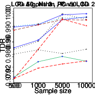
Figure 11:

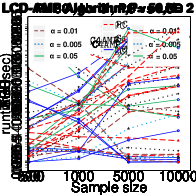
Figure 12: First two columns show the performance of the decomposition based (LCD-AMP), original PC-like and Stable-PC4AMP algorithms for randomly generated Gaussian chain graph models: average over 30 repetitions with 50 variables correspond to N = 2, 3, and the significance level $\alpha=0.005$. In each plot, the solid blue line corresponds to the LCD-AMP  algorithm, the dashed red line corresponds to the original PC-like algorithm, and the dotted grey line corresponds to the stable PC-like (Stable-PC4AMP) algorithm. The third column shows the performance of the decomposition-based (LCD-AMP) algorithm for randomly generated Gaussian chain graph models: average over 30 repetitions with 50 variables correspond to N = 2, and significance levels $\alpha=0.05,0.01,0.005$. In each plot, the solid green line corresponds to $\alpha=0.05$, the dashed brown line corresponds to $\alpha=0.01$, and the dotted blue line corresponds to $\alpha=0.005$.

Figure 13: First two columns show the running times of the decomposition-based (LCD-AMP), original PC-like and Stable-PC4AMP algorithms for randomly generated Gaussian chain graph models: average over 30 repetitions with 50 variables correspond to N = 2,3 and significance levels $\alpha=0.005$. In each plot, the solid blue line corresponds to the LCD-AMP  algorithm, the dashed red line corresponds to the original PC-like algorithm, and the dotted grey line corresponds to the Stable-PC4AMP algorithm. The third column shows the running times of the decomposition-based (LCD-AMP) algorithm for randomly generated Gaussian chain graph models: average over 30 repetitions with 50 variables correspond to N = 2, and significance levels $\alpha=0.05,0.01,0.005$. In each plot, the solid green line corresponds to $\alpha=0.05$, the dashed brown line corresponds to $\alpha=0.01$, and the dotted blue line corresponds to $\alpha=0.005$.

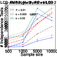
Figure 14: First two columns show the number of independence tests used by the decomposition-based (LCD-AMP), original PC-like and Stable-PC4AMP algorithms for randomly generated Gaussian chain graph models: average over 30 repetitions with 50 variables corresponding to average degrees N = 2,3 and significance level $\alpha=0.005$. In each plot, the solid blue line corresponds to the LCD-AMP  algorithm, the dashed red line corresponds to the original PC-like algorithm, and the dotted grey line corresponds to the Stable-PC4AMP algorithm. The third column shows the number of independence tests used by the decomposition-based (LCD-AMP) algorithm for randomly generated Gaussian chain graph models: average over 30 repetitions with 50 variables corresponding to average degree N = 2, and significance levels $\alpha=0.05,0.01,0.005$. In each plot, the solid green line corresponds to $\alpha=0.05$, the dashed brown line corresponds to $\alpha=0.01$, and the dotted blue line corresponds to $\alpha=0.005$.

Results

The experimental results in Figure 12 shows that:

• Both algorithms work well on sparse graphs $(N=2,3)$.

• For both algorithms, typically the TPR, TDR, and ACC increase with sample size.

• The SHD and FPR decrease with sample size.

• A large significance level $(\alpha=0.05)$ typically yields large TPR, FPR, and SHD.

• In almost all cases, the performance of the LCD-AMP algorithm based on all error measures i.e., TPR, FPR, TDR, ACC, and SHD is better than the performance of the PC-like and Stable-PC4AMP algorithms.

• In most cases, error measures based on $\alpha=0.01$ and $\alpha=0.005$ are very close. Generally, our empirical results suggests that in order to obtain a better performance, we can choose a small value (say $\alpha=0.005$ or 0.01) for the significance level of individual tests along with large sample if at all possible. However, the optimal value for a desired overall error rate may depend on the sample size, significance level, and the sparsity of the underlying graph.

• While the Stable-PC4AMP algorithm has a better TDR and FPR in comparison with the original PC-like algorithm, the original PC-like algorithm has a better TPR as observed in the case of DAGs (Colombo and Maathuis, 2014). This can be explained by the fact that the Stable-PC4AMP algorithm tends to perform more tests than the original PC-like algorithm.

• There is no meaningful difference between the performance of the Stable-PC4AMP algorithm and the original PC-like algorithm in terms of error measures ACC and SHD.

When considering average running times versus sample sizes, as shown in Figures 13, we observe that:

• The average run time increases when sample size increases.

• The average run times based on $\alpha=0.01$ and $\alpha=0.005$ are very close and in all cases better than $\alpha=0.05$, while choosing $\alpha=0.005$ yields a consistently (albeit slightly) lower average run time across all the settings.

• Generally, the average run time for the decomposition-based algorithm is lower than that for the ( Stable-) PC-like algorithm.

In Figure 14, the algorithms are compared by counting the number of independence tests, rather than runtime, in order to reduce the impact of different implementations (R packages). We observe that:

• The average number of independence tests increases when sample size increases.

• The average number of independence tests based on $\alpha=0.01$ and $\alpha=0.005$ are close and in all cases better than $\alpha=0.05$, while choosing $\alpha=0.005$ yields a consistently lower average number of independence tests across all the settings.

• Generally, the average number of independence tests for the decomposition-based algorithm is better than that for the (Stable-) PC-like algorithm.

These observations are consistent with the theoretical complexity analysis that we discussed in Section 5.3. In fact, our findings confirm that the decomposition-based algorithm reduces complexity and increases the power of computational independence tests.

6.2.3 Experimental Results in High-Dimensional Settings

Although the results in Figure 15 show that our proposed modifications of PC-like, i.e., Stable-PC4AMP, Conservative-PC4AMP, and Stable-Conservative-PC4AMP provide stabler estimations and closer to the true underlying structure in sparse high-dimensional settings for simulated Gaussian data compared with PC-like, we are interested to test whether the difference is statistically significant.

Experimental Setting

To show that the order-dependence of PC-like algorithm is problematic in high-dimensional data, we compared the SHD of the original PC-like algorithm against its modifications for randomly generated Gaussian chain graph models: average over 30 repetitions with 1000 variables with $N=2$, sample size $S=50$, and the significance level $\alpha=0.05,0.01,0.005,0.001$. We used an independent t-test to quantitatively evaluate whether the means of SHDs in different structure discovery algorithms are different.

Results

The t-test results in Tables 5 and 6 show that:

• Except for the p-value $\alpha=0.001$, the mean SHD of our proposed algorithms (i.e., Stable-PC4AMP, Conservative-PC4AMP, and Stable-Conservative-PC4AMP) is significantly different (lower) from the mean of PC-like’s SHD. This confirms that our proposed modifications provide more reliable and better-learned structures in comparison with the PC-like algorithm.

• The mean of Stable-Conservative-PC4AMP’s SHD is significantly different from the mean of Stable-PC4AMPand Conservative-PC4AMPalgorithms’ SHD for the p-value $\alpha=0.05$. However, for the other p-values the difference is not meaningful.

• Taken together, the quantitative t-test analysis confirms what one would expect from visual inspection of Figure 15.

In addition to t-test, we also performed F-test to test statistical difference between the corresponding pairwise SHD variances. Our results show that the p-value of F-test in all pairwise comparisons between all algorithms (Stable-PC4AMP,Conservative-PC4AMP, Stable-Conservative-PC4AMP, and PC-like) is greater than the significance level $\alpha=0.05$. In conclusion, there is no significant difference between the variances of the pairwise SHDs. The similarity of SHD variances indicates that requiring stability does not control error propagation in constraint-based algorithms, and that there remains a common source of errors to be discovered in future work.

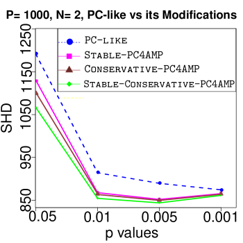
Figure 15: The SHD of the original PC-like algorithm against its modifications for randomly generated Gaussian chain graph models: average over 30 repetitions with 1000 variables correspond to $N=2$, sample size $S=50$, and the significance level $\alpha=0.05,0.01,0.005,0.001$.

Table 5: P-values for pairwise t-tests. Bold numbers in the table mean that PC-like’s average SHD is significantly different from other’s average SHD with the given p-value ($\alpha$).

	PC-like	PC-like	PC-like	PC-like
	($\alpha=0.05$)	($\alpha=0.01$)	($\alpha=0.005$)	($\alpha=0.001$)
Stable-PC4AMP	$\mathbf{7.84\mathrm{e}{-11}}$	$\mathbf{3.338\mathrm{e}{-06}}$	$\mathbf{0.0001399}$	$0.1781$
Conservative-PC4AMP	$\mathbf{9.8\mathrm{e}{-13}}$	$\mathbf{1.682\mathrm{e}{-05}}$	$\mathbf{0.001254}$	0.6045
Stable-Conservative-PC4AMP	$\mathbf{4.997\mathrm{e}{-16}}$	$\mathbf{7.368\mathrm{e}{-07}}$	$\mathbf{0.0001269}$	0.3511

Table 6: P-values for pairwise t-tests. Bold numbers in the table mean that the average SHD is significantly different when executing the given pair of algorithms for the p-value $\alpha=0.05$.

	Stable-	Conservative-	Stable-Conservative-
	PC4AMP	PC4AMP	PC4AMP
Stable-PC4AMP	-	0.116	$\mathbf{0.0003893}$
Conservative-PC4AMP	0.116	-	$\mathbf{0.04492}$
Stable-Conservative-PC4AMP	$\mathbf{0.0003893}$	$\mathbf{0.04492}$	-

6.3 Performance on Discrete Bayesian Networks

Since Bayesian networks are special cases of AMP CGs, it is of interest to see whether our proposed algorithms still work well when the data are actually generated from a Bayesian network. This matters because we often do not have the information that the underlying graph is a DAG, which is usually untestable from data alone. For this purpose, we perform simulation studies for four well-known Bayesian networks from Bayesian Network Repository (Scutari, 2017): ASIA, INSURANCE, ALARM, and HAILFINDER. We purposefully selected these networks because they have different sizes (from small to large numbers of nodes, edges, and parameters), and they are often used to evaluate structure learning algorithms. We briefly introduce these networks here:

• ASIA (Lauritzen and Spiegelhalter, 1988) with 8 nodes, 8 edges, and 18 parameters, it describes the diagnosis of a patient at a chest clinic who may have just come back from a trip to Asia and may be showing dyspnea. Standard constraint-based learning algorithms are not able to recover the true structure of the network because of the presence of a functional node.

• INSURANCE (Binder et al., 1997) with 27 nodes, 52 edges, and 984 parameters, it evaluates car insurance risks.

• ALARM (Beinlich et al., 1989) with 37 nodes, 46 edges and 509 parameters, it was designed by medical experts to provide an alarm message system for intensive care unit patients based on the output a number of vital signs monitoring devices.

• HAILFINDER (Abramson et al., 1996) with 56 nodes, 66 edges, and 2656 parameters, it was designed to forecast severe summer hail in northeastern Colorado.

We compared the performance of our algorithms for these Bayesian networks for significance level $\alpha=0.05$. The Structural Hamming Distance (SHD) compares the structure of the largest deflagged of the learned and the original networks, for a fair comparison.

Table 7: Results for discrete samples from the ASIA (5000 observations), INSURANCE (20000 observations), ALARM (20000 observations), and HAILFINDER (20000 observations) networks from the bnlearn R package respectively. Each row corresponds to the significance level: $\alpha=0.05$. In order to learn an undirected independence graph from a given data set in the LCD-AMP  algorithm we used the Incremental Association with FDR (IAMB-FDR) algorithm (Peña, 2008) from the bnlearn R package (Scutari, 2017) and the stepwise forward selection (FWD-AIC or FWD-BIC) algorithms in (de Abreu et al., 2010a).

Algorithm	TPR	TDR	FPR	ACC	SHD
LCD-AMP  Algorithm (IAMB-FDR)	0.5	0.8	0.05	0.821	7
LCD-AMP  Algorithm (FWD-AIC)	0.75	1	0	0.929	3
LCD-AMP  Algorithm (FWD-BIC)	0.875	1	0	0.964	1
Stable-PC4AMP Algorithm	0.5	1	0	0.8571	5
Original PC-like Algorithm	0.5	1	0	0.8571	5
LCD-AMP  Algorithm (IAMB-FDR)	0.558	0.935	0.0067	0.929	33
LCD-AMP  Algorithm (FWD-AIC)	0.385	0.952	0.0033	0.906	42
LCD-AMP Algorithm (FWD-BIC)	0.538	0.875	0.0134	0.920	36
Stable-PC4AMP Algorithm	0.173	1	0	0.877	43
Original PC-like Algorithm	0.346	1	0	0.903	41
LCD-AMP  Algorithm (IAMB-FDR)	0.783	0.878	0.0081	0.977	24
LCD-AMP  Algorithm (FWD-AIC)	0.696	0.914	0.0048	0.974	27
LCD-AMP  Algorithm (FWD-BIC)	0.760	0.921	0.0048	0.979	20
Stable-PC4AMP Algorithm	0.587	1	0	0.971	25
Original PC-like Algorithm	0.696	1	0	0.979	18
LCD-AMP  Algorithm (IAMB-FDR)	0.515	0.971	0.00068	0.979	40
LCD-AMP  Algorithm (FWD-AIC)
LCD-AMP  Algorithm (FWD-BIC)	0.803	0.930	0.0027	0.989	38
Stable-PC4AMP Algorithm	0.394	1	0	0.974	46
Original PC-like Algorithm	0.455	0.811	0.0047	0.972	49

6.3.1 Experimental Results

The results of comparing all learning methods in Table 7 indicate that the performance of LCD-AMP  algorithm in many cases is better than that of the PC-like and Stable-PC4AMP algorithms. In particular, we observed:

• Although the performance of our LCD-AMP  algorithm, overall, is better than the PC-like and Stable-PC4AMP algorithms, it is highly variable depending on the procedure that is used for the UIG discovery, especially in TPR and SHD. One of the most important implications of this observation is that there is much room for improvement to the UIG recovery algorithms and decomposition-based learning algorithms, and hopefully the present paper will inspire other researchers to address this important class of algorithms. In general, the more accurate the UIG discovery algorithm, the more robust the result. In our experiments, generally, the IAMB-FDR  algorithm (Peña, 2008) and the stepwise forward selection (FWD-BIC) algorithm (de Abreu et al., 2010a) are more effective as a preliminary step (UIG recovery) towards understanding the overall dependence structure of high-dimensional discrete data.

• The PC-like and Stable-PC4AMP algorithms tend to have better TDR and FPR. This comes at the expense, however, of much worse TPR. This suggests that the PC-like and Stable-PC4AMP algorithms tend to add too many edges to the skeleton of the learned graph.

7 Related Work

The contributions of this paper regarding finding minimal separators and structure learning algorithms intersect with various works in the literature as follows.

7.1 Finding Minimal Separators in Probabilistic Graphical Models

A challenging task of model testing is to detect for any given pair of nodes a minimal or minimum separator. Nontrivial algorithms for testing and for finding a minimal $d$-separator in a DAG were first proposed in (Acid and de Campos, 1996; Tian et al., 1998). An algorithm for learning the structure of Bayesian networks from data, based on the idea of finding minimal $d$-separating sets, proposed in (Acid and de Campos, 2001). In (van der Zander and Liskiewicz, 2019), the authors show that testing and finding a minimal separator in DAGs can be done in linear time. As shown in (van der Zander and Liskiewicz, 2019; van der Zander et al., 2019), (minimal) separating sets have important applications in causal inference tasks like finding (minimal) covariate adjustment sets or conditional instrumental variables. In (Javidian and Valtorta, 2018a, b), the authors proposed algorithms for testing and for finding a minimal separator in an LWF CG and an MVR CG, respectively. In this paper, we proposed algorithms for testing and finding minimal separators in AMP chain graphs (see Section 3).

7.2 PC-like Algorithms for Probabilistic Graphical Models

The PC algorithm proposed by Peter Spirtes and Clark Glymour (Spirtes et al., 2000) learns the Bayesian network structure from data by testing for conditional independence between various sets of variables. Given the results of these tests, a network pattern is constructed so that the Markov property holds and $d$-separation confirms the resulting graph mirroring those conditional independencies found in the data. The PC algorithm consists of two phases: In the first phase, an undirected graph is learned. This is known as the skeleton of the Bayesian network. In the second phase, arrowheads are added to some of the edges where they can be inferred. The output graph may not be fully oriented and is called a pattern. When the pattern contains undirected edges, these indicate that the data are consistent with models in which either orientation is possible.

The PC algorithm is known to be order-dependent, in the sense that the output can depend on the order in which the variables are given. This order-dependence can be very pronounced in high-dimensional settings, where it can lead to highly variable results. In order to resolve the order-dependence problem, Colombo and Maathuis (Colombo and Maathuis, 2014) proposed several modifications of the PC algorithm that remove part or all of this order-dependence.

PC-like algorithms currently exist for all three chain graph interpretations (Javidian, 2019; Peña, 2012; Sonntag and Peña, 2012) where the different phases are slightly altered according to the interpretation but the basic ideas are kept the same. The first phase finds the adjacencies (skeleton), the second orients the edges that must be oriented the same in every CG in the Markov equivalence class and the third phase transforms this graph into a CG. Order-independent versions of the PC-like algorithm for LWF CGs and MVR CGs were proposed in (Javidian, 2019; Javidian et al., 2019), respectively. In this paper, we proved that the proposed PC-like algorithm for AMP CGs in (Peña, 2012) is order-dependent. Then, we proposed several modifications of the PC-like algorithm that remove part or all of this order-dependence, but the proposed algorithms do not change the result when perfect conditional independence information is used (see Section 4).

7.3 Decomposition Based Learning (LCD-Like) Algorithms for PGMs

Structure learning of Bayesian networks via decomposition was proposed in (Xie et al., 2006). This approach starts with finding a decomposition of the entire variable set into subsets, on each of which the local skeleton is then recovered. In the next phase, the adjacency graph (global skeleton) is reconstructed by merging the decomposed graphs (local skeletons) together. In the last phase, arrowheads are added to some of the edges where they can be inferred in an efficient manner with lower complexity than the PC algorithm (Xie et al., 2006).

Following the same idea, a decomposition-based algorithm called LCD (Learn Chain graphs via Decomposition) was proposed in (Ma et al., 2008; Javidian, 2019) to learn LWF CGs and MVR CGs, respectively; where the different phases are slightly altered according to the interpretation but the basic ideas in (Xie et al., 2006) are kept the same. In this paper, we developed an LCD-like algorithm, called LCD-AMP , for learning the structure of AMP chain graphs based on the idea of decomposing the learning problem into a set of smaller scale problems on its decomposed subgraphs. Similarities and differences between LCD-AMP  and other LCD-like algorithms are discussed in Section 5.

8 Conclusion

This paper addresses two main problems in the context of AMP chain graphs (CGs): finding minimal separators and structure learning. We first studied and solved the problem of finding minimal separating sets for pairs of variables in an AMP CGs. We also studied some extensions of the basic problem that include finding a minimal separator from a restricted set of nodes, finding a minimal separator for two given disjoint sets, testing whether a given separator is minimal, and listing all minimal separators, given two non-adjacent nodes (or disjoint subsets) $X$ and $Y$. Applications of this research include: (1) learning chain graphs from data and (2) problems related to the selection of the variables to be instantiated when using chain graphs for inference tasks, a topic for future work.

Experimental evaluations in the Gaussian case show that both (Stable-) PC-like  and LCD-AMP algorithms yield good results when the underlying graph is sparse; this holds also in the discrete case, according to experiments with standard benchmark Bayesian networks. This is important because Bayesian networks are special cases of AMP CGs and we often do not know the information that the true underlying structure is a DAG, which is not usually testable from data. The LCD-AMP algorithm achieves competitive results with the PC-like and Stable-PC4AMP learning algorithms in both the Gaussian and discrete cases. In fact, our LCD-AMP  usually outperforms the PC-like and Stable-PC4AMP algorithms in all five performance metrics i.e., TPR, FPR, TDR, ACC, and SHD.

The local skeletons of our LCD-AMP  algorithm and CI tests at each level of the skeleton recovery of the Stable-PC4AMP algorithm can be learned independently from each other, and later merged and reconciled to produce a coherent AMP chain graph. This allows the parallel implementations for scaling up the task of learning AMP chain graphs from data containing more than hundreds of variables, which is crucial for big data analysis tasks. The correctness proof of the decomposition-based algorithm (i.e., LCD-AMP) is built upon our results on separating sets. This algorithm exhibits reduced complexity, as measured by run time and number of conditional independence tests, enhances the power of conditional independence tests by reducing the number of separating sets that need to be considered, and, according to our experimental evaluation, achieves better quality with respect to the learned structure.

A direction for future work is the design of a hybrid algorithm for learning AMP chain graphs that exploits minimal separators directly, as done in (Acid and de Campos, 2001) for learning Bayesian networks. Another natural continuation of the work presented here would be to develop a learning algorithm with weaker assumptions than the faithfulness assumption. This could for example be a learning algorithm that only assumes that the probability distribution satisfies the composition property. It should be mentioned that (Peña et al., 2014) developed an algorithm for learning LWF CGs under the composition property. However, (Peña, 2014a) proved that the same technique cannot be used for AMP chain graphs. We believe that our decomposition-based approach is extendable to the structural learning of marginal AMP chain graphs (Peña and Gómez-Olmedo, 2016) and ancestral graphs (Richardson and Spirtes, 2002). Also, a potential continuation of the work presented here would be to develop a learning algorithm via decomposition for marginal AMP chain graphs and ancestral graphs under the faithfulness assumption. As we mentioned before, our LCD-AMP algorithm works better than the (Stable-) PC-like in many settings. The reason is that LCD-AMP algorithm takes advantage of local computations that makes it robust against the choice of learning parameters. In Bayesian networks, the concept that enables us to take advantage of local computation is Markov blanket. Recently, (Javidian et al., 2020) extended the concept of Markov blankets to LWF CGs and proved what variables make up the Markov blanket of a target variable in an LWF CG. Characterizing Markov blankets in AMP CGs and designing a Markov blanket based algorithm for learning AMP CGs nother interesting direction for future work.

Appendix A. Proofs of Theorems 15 and 16

In Theorem 9, we showed that if we find a separator over $S$ in $(G_{ant(u\cup v)})^{a}$ then it is a $p$-separator in $G$. On the other hand, if there exists a $p$-separator over $S$ in $G$ then there must exist a separator over $S$ in $(G_{ant(u\cup v)})^{a}$ by removing all nodes which are not in $ant(u\cup v)$ from it. This observation yield the following results.

Lemma 18

Let $u$ and $v$ be two non-adjacent vertices in AMP CG $G$, and let $\rho$ be a chain from $u$ to $v$. If $\rho$ is not contained in $ant(u\cup v)$, then $\rho$ is blocked by any subset $S$ of $ant(u\cup v)\setminus\{u,v\}$.

Proof  Since $\rho\not\subseteq ant(u\cup v)$, there is a sequence from $s$ (may be $u$) to $y$ (may be $v$) in $\rho=(u,\dots,s,t,\dots,x,y,\dots,v)$ such that $s$ and $y$ are contained in $ant(u\cup v)$ and all vertices from $t$ to $x$ are out of $ant(u\cup v)$.Then the edges $s-t$ and $x-y$ must be oriented as $s\to t$ and $x\leftarrow y$, otherwise $t$ or $x$ belongs to $ant(u\cup v)$. Thus there exist at least one triplex between $s$ and $y$ on $\rho$. The middle vertex $w$ of the triplex closest to $s$ between $s$ and $y$ is not contained in $ant(u\cup v)$, and any descendant of $w$ is not in $ant(u\cup v)$. So $\rho$ is blocked by this triplex, and it cannot be activated conditionally on any vertex in $S$ where $S\subseteq ant(u\cup v)\setminus\{u,v\}$.  

Lemma 19

Let $T$ be a $p$-separation tree for the AMP CG $G$. For any vertex $u$ there exists at least one node of $T$ that contains $u$ and $pa(u)$.

Proof  If $pa(u)$ is empty, the result is trivial. Otherwise let $C$ denote the node of $T$ which contains $u$ and the most elements of $u$’s parent. Since no set can separate $u$ from a parent, there must be a node of $T$ that contains $u$ and the parent. If $u$ has only one parent, then we obtain the lemma. If $u$ has two or more parents, we choose two arbitrary elements $v$ and $w$ of $u$’s parent that are not contained in a single node of $T$ but are contained in two different nodes of $T$, say $\{u,v\}\subseteq C$ and $\{u,w\}\subseteq C^{\prime}$ respectively, since all vertices in $V$ appear in $T$. On the chain from $C$ to $C^{\prime}$ in $T$, all separators must contain $u$, otherwise they cannot separate $C$ from $C^{\prime}$. However, any separator containing $u$ cannot separate $v$ and $w$ because $v\to u\leftarrow w$ is an active triplex between $v$ and $w$ in $G$. Thus we got a contradiction.  

Lemma 20

Let $T$ be a $p$-separation tree for AMP CG $G$ and $C$ a node of $T$. If $u$ and $v$ are two vertices in $C$ that are non-adjacent in $G$ and belong to two different chain components, then there exists a node $C^{\prime}$ of $T$ containing $u,v$ and a set $S$ such that $S$ $p$-separates $u$ and $v$ in $G$.

Proof  Assume that $u$ and $v$ are two vertices in $G$ that are non-adjacent and belong to two different chain components. Without loss of generality, we can suppose that $v$ is not a descendant of the vertex $u$ in $G$, i.e., $v\not\in nd(u)$. According to the pairwise Markov property for AMP chain graphs in (Andersson et al., 2001), $u\perp\!\!\!\perp v|pa(u).$ By Lemma 19, there is a node $C_{1}$ of $T$ that contains $u$ and $pa(u)$. If $v\in C_{1}$, then $S$ defined as the parents of $u$ $p$-separates $u$ from $v$.

If $v\not\in C_{1}$, choose the node $C_{2}$ that is the closest node in $T$ to the node $C_{1}$ and that contains $u$ and $v$. Consider that there is at least one parent $p$ of $u$ that is not contained in $C_{2}$. Thus there is a separator $K$ connecting $C_{2}$ toward $C_{1}$ in $T$ such that $K$ $p$-separates $p$ from all vertices in $C_{2}\setminus K$. Note that on the chain from $C_{1}$ to $C_{2}$ in $T$, all separators must contain $u$, otherwise they cannot separate $C_{1}$ from $C_{2}$. So, we have $u\in K$ but $v\not\in K$ (if $v\in K$, then $C_{2}$ is not the closest node of $T$ to the node $C_{1}$). In fact, for every parent $p^{\prime}$ of $u$ that is contained in $C_{1}$ but not in $C_{2}$, $K$ separates $p^{\prime}$ from all vertices in $C_{2}\setminus K$, especially the vertex $v$.

Define $S=[ant(u\cup v)\cap(K\cup\{p\in pa(u)|p\in C_{2}\})]\setminus\tau_{u}$, where $\tau_{u}$ is the chain component that includes $u$. It is not difficult to see that $S$ is a subset of $C_{2}$. We need to show that $u$ and $v$ are $p$-separated by $S$, that is, every chain between $u$ and $v$ in $G$, say $\rho$, is blocked by $S$.

If $\rho$ is not contained in $ant(u\cup v)$, then we obtain from Lemma 18 that $\rho$ is blocked by $S$.

When $\rho$ is contained in $ant(u\cup v)$, let $x$ be adjacent to $u$ on $\rho$, that is, $\rho=(u,x,y,\dots,v)$. We consider the three possible orientations of the edge between $u$ and $x$. We now show that $\rho$ is blocked in all three cases by $S$.

• $u\leftarrow x$, so it is obvious that $x$ is not a triplex node and we have two possible sub-cases:

  1. $x\in C_{2}$. In this case the chain $\rho$ is blocked at $x$.

  2. $x\not\in C_{2}$. In this case $K$ $p$-separates $x$ from $v$. Theorem 9 guarantees that the set $S^{\prime}=K\cap ant(x\cup v)$ also $p$-separates $x$ from $v$. Note that $S^{\prime}\cap\tau_{u}=\emptyset$ to prevent a partially directed cycle, and $S^{\prime}\subseteq S$. So, $S$ $p$-separates $x$ from $v$ i.e., the chain between $v$ and $x$ is blocked by $S$. Hence the chain $\rho$ is blocked by $S$.

• $u\to x$. We have the following sub-cases:

  1. $x\in ant(u)$. This case is impossible because a partially directed cycle would occur.

  2. $x\in an(v)$. This case is impossible because $v$ cannot be a descendant of $u$.

• $u\mathrel{\leavevmode\hbox to14.63pt{\vbox to0.4pt{\text{[drawing]}}}}x$, so $x\in\tau_{u}$. In this case the chain $\rho$ between $u$ and $v$ has a triplex node at $y\in\tau_{u}$ that is not in $S$. So, the chain $\rho$ is blocked at $y$ and cannot be activated by $S$.

 

Proof [Proof of Theorem 15] From (Cowell et al., 1999), we know that any separator $S$ in junction tree $T$ separates $V_{1}\setminus S$ and $V_{2}\setminus S$ in the triangulated graph $\bar{G}_{V}^{t}$, where $V_{i}$ denotes the variable set of the subtree $T_{i}$ induced by removing the edge with a separator $S$ attached, for $i=1,2$. Since the edge set of $\bar{G}_{V}^{t}$ contains that of undirected independence graph $\bar{G}_{V}$ for $G$, $V_{1}\setminus S$ and $V_{2}\setminus S$ are also separated in $\bar{G}_{V}$. Since $\bar{G}_{V}$ is an undirected independence graph for $G$, using the definition of $p$-separation tree we obtain that $T$ is a $p$-separation tree for $G$.  

Proof [Proof of Theorem 16] ($\Rightarrow$) If condition (i) is the case, nothing remains to prove. Otherwise, Lemma 20 implies condition (ii).

($\Leftarrow$) Assume that $u$ and $v$ are not contained together in any chain component and any node $C$ of $T$. Also, assume that $C_{1}$ and $C_{2}$ are two nodes of $T$ that contain $u$ and $v$, respectively. Consider that $C_{1}^{\prime}$ is the most distant node from $C_{1}$, between $C_{1}$ and $C_{2}$, that contains $u$ and $C_{2}^{\prime}$ is the most distant node from $C_{2}$, between $C_{1}$ and $C_{2}$, that contains $v$. Note that it is possible that $C_{1}^{\prime}=C_{1}$ or $C_{2}^{\prime}=C_{2}$. By the condition (i) we know that $C_{1}^{\prime}\neq C_{2}^{\prime}$. The sufficiency of condition (i) is given by the definition of the $p$-separation tree, because any separator between $C_{1}^{\prime}$ and $C_{2}^{\prime}$ $p$-separates $u$ from $v$.

The sufficiency of conditions (ii) is trivial by the definition of $p$-separation.  

The following example shows that Theorem 16 cannot be strengthened.

(a)

(b)

(c)

(d)

Figure 16: (a) AMP CG $G$, (b) augmented graph $G^{a}$, (c) triangulated graph $(G^{a})^{t}$, and (d) p-separation tree $T$.

Example 7

Consider the AMP CG $G$ in Figure 16(a). Vertices $f$ and $h$ are not adjacent but both of them belong to the same chain component. As one can see in the Figure 16(d), vertices $f$ and $h$ belong to nodes tree $C_{1}=\{b,c,d,f,g,h\}$ and $C_{2}=\{a,b,d,e,f,h\}$. However, none of them contains a subset of $V_{G}$ that $p$-separates $f$ from $h$.

Proof  [Correctness of Algorithm 6] By the definition of p-separation trees and Theorem 16, the initializations at local and global skeleton recovery phases guarantee that no edge is created between any two variables which are not in the same node of the $p$-separation tree. Also, deleting edges at local and global skeleton recovery phases guarantees that any other edge between two $p$-separated variables can be deleted in some local skeleton or in the removal procedure at the global skeleton recovery phase. Thus the global skeleton obtained after line 22 is correct. Note that, in an AMP CG, every missing edge corresponds to at least one independency in the corresponding independence model. Therefore, each augmented edge $u\mathrel{\leavevmode\hbox to14.63pt{\vbox to0.4pt{\text{[drawing]}}}}v$ in the undirected independence graph must be deleted at some subgraph over a node of the $p$-separation tree or at some point of the removal procedure of the global skeleton recovery. The proof of the correctness of orientation rules R1-R4 can be found in (Peña, 2012).

References

- Abramson et al. (1996) Bruce Abramson, John Brown, Ward Edwards, Allan Murphy, and Robert L. Winkler. Hailfinder: A Bayesian system for forecasting severe weather. International Journal of Forecasting, 12(1):57 – 71, 1996. Probability Judgmental Forecasting.
- Acid and de Campos (1996) Silvia Acid and Luis M. de Campos. An algorithm for finding minimum d-separating sets in belief networks. Proceedings of the Twelfth international conference on Uncertainty in artificial intelligence, pages 3–10, 1996.
- Acid and de Campos (2001) Silvia Acid and Luis M. de Campos. A hybrid methodology for learning belief networks: Benedict. International Journal of Approximate Reasoning, 27(3):235–262, 2001.
- Anandkumar et al. (2012) Animashree Anandkumar, Vincent Y. F. Tan, Furong Huang, and Alan S. Willsky. High-dimensional structure estimation in Ising models: Local separation criterion. Ann. Statist., 40(3):1346–1375, 06 2012. doi: 10.1214/12-AOS1009. URL https://doi.org/10.1214/12-AOS1009.
- Andersson and Perlman (2006) Steen A. Andersson and Michael D. Perlman. Characterizing Markov equivalence classes for AMP chain graph models. The Annals of Statistics, 34(2):939–972, 04 2006.
- Andersson et al. (1996) Steen A. Andersson, David Madigan, and Michael D. Perlman. An alternative Markov property for chain graphs. In Eric Horvitz and Finn V. Jensen, editors, Proceedings of the Twelfth Conference on Uncertainty in artificial intelligence, pages 40–48, 1996.
- Andersson et al. (2001) Steen A. Andersson, David Madigan, and Michael D. Perlman. Alternative Markov properties for chain graphs. Scandinavian Journal of Statistics, 28(1):33–85, 2001.
- Andrews et al. (2018) Bryan Andrews, Joseph Ramsey, and Gregory F Cooper. Scoring Bayesian networks of mixed variables. International journal of data science and analytics, 6(1):3–18, 2018.
- Banerjee et al. (2008) Onureena Banerjee, Laurent El Ghaoui, and Alexandre d’Aspremont. Model selection through sparse maximum likelihood estimation for multivariate Gaussian or binary data. Journal of Machine Learning Research, 9:485–516, 2008.
- Beinlich et al. (1989) Ingo A. Beinlich, H. J. Suermondt, R. Martin Chavez, and Gregory F. Cooper. The alarm monitoring system: A case study with two probabilistic inference techniques for belief networks. In Jim Hunter, John Cookson, and Jeremy Wyatt, editors, AIME 89, pages 247–256, Berlin, Heidelberg, 1989. Springer Berlin Heidelberg.
- Berry et al. (2004) Anne Berry, Jean Blair, Pinar Heggernes, and Barry Peyton. Maximum cardinality search for computing minimal triangulations of graphs. Algorithmica, 39:287–298, 2004.
- Binder et al. (1997) John Binder, Daphne Koller, Stuart Russell, and Keiji Kanazawa. Adaptive probabilistic networks with hidden variables. Machine Learning, 29(2):213–244, Nov 1997.
- Bresler et al. (2008) Guy Bresler, Elchanan Mossel, and Allan Sly. Reconstruction of Markov random fields from samples: Some observations and algorithms. In Ashish Goel, Klaus Jansen, José D. P. Rolim, and Ronitt Rubinfeld, editors, Approximation, Randomization and Combinatorial Optimization. Algorithms and Techniques, pages 343–356, Berlin, Heidelberg, 2008. Springer Berlin Heidelberg. ISBN 978-3-540-85363-3.
- Bromberg et al. (2009) Facundo Bromberg, Dimitris Margaritis, and Vasant Honavar. Efficient Markov network structure discovery using independence tests. J. Artif. Int. Res., 35(1):449–484, July 2009. ISSN 1076-9757.
- Chow and Liu (1968) C. Chow and C. Liu. Approximating discrete probability distributions with dependence trees. IEEE Transactions on Information Theory, 14(3):462–467, May 1968. ISSN 1557-9654. doi: 10.1109/TIT.1968.1054142.
- Colombo and Maathuis (2014) Diego Colombo and Marloes H. Maathuis. Order-independent constraint-based causal structure learning. The Journal of Machine Learning Research, 15(1):3741–3782, 2014.
- Cooper (1990) Gregory F. Cooper. The computational complexity of probabilistic inference using Bayesian belief networks. Artificial Intelligence, 42(2):393 – 405, 1990. ISSN 0004-3702. doi: https://doi.org/10.1016/0004-3702(90)90060-D. URL http://www.sciencedirect.com/science/article/pii/000437029090060D.
- Cormen et al. (2009) Thomas H. Cormen, Charles E. Leiserson, Ronald L. Rivest, and Clifford Stein. Introduction to Algorithms, Third Edition. The MIT Press, 3rd edition, 2009. ISBN 0262033844, 9780262033848.
- Cowell et al. (1999) R. Cowell, A. P. Dawid, S. Lauritzen, and D. J. Spiegelhalter. Probabilistic networks and expert systems. Statistics for Engineering and Information Science. Springer-Verlag, 1999.
- Cox and Wermuth (1993) D. R. Cox and Nanny Wermuth. Linear dependencies represented by chain graphs. Statistical Science, 8(3):204–218, 1993.
- Cox and Wermuth (1996) D. R. Cox and Nanny Wermuth. Multivariate Dependencies-Models, Analysis and Interpretation. Chapman and Hall, 1996.
- de Abreu et al. (2010a) Gabriel de Abreu, Rodrigo Labouriau, and David Edwards. High-dimensional graphical model search with the graphd R package. Journal of Statistical Software, Articles, 37(1):1–18, 2010a. ISSN 1548-7660. doi: 10.18637/jss.v037.i01. URL https://www.jstatsoft.org/v037/i01.
- de Abreu et al. (2010b) Gabriel de Abreu, Rodrigo Labouriau, and David Edwards. Selecting high-dimensional mixed graphical models using minimal AIC or BIC forests. BMC Bioinformatics, 11(18), 2010b. ISSN 1548-7660. doi: 10.18637/jss.v037.i01. URL https://www.jstatsoft.org/v037/i01.
- Drton (2009) Mathias Drton. Discrete chain graph models. Bernoulli, 15(3):736–753, 2009.
- Edelkamp and Schroedl (2011) Stefan Edelkamp and Stefan Schroedl. Heuristic Search: Theory and Applications. Morgan Kaufmann Publishers Inc., San Francisco, CA, USA, 2011.
- Edwards (2000) D. Edwards. Introduction to Graphical Modelling. 2nd Ed. Springer-Verlag, New York, 2000.
- Fenton and Neil (2018) Norman Fenton and Martin Neil. Risk Assessment and Decision Analysis with Bayesian Networks. Chapman and Hall/CRC, New York, 2nd edition, 2018.
- Frydenberg (1990) Morten Frydenberg. The chain graph Markov property. Scandinavian Journal of Statistics, 17(4):333–353, 1990.
- Højsgaard et al. (2012) S. Højsgaard, D. Edwards, and S. Lauritzen. Graphical Models with R. Springer, 2012.
- Javidian and Valtorta (2018a) M. A. Javidian and M. Valtorta. Finding minimal separators in LWF chain graphs. In The 9th International Conference on Probabilistic Graphical Models (PGM 2018), pages 193–200, 2018a.
- Javidian and Valtorta (2018b) M. A. Javidian and M. Valtorta. Finding minimal separators in ancestral graphs. In Seventh Causal Inference Workshop at the 34th Conference on Artifical Intelligence (UAI-18), 2018b.
- Javidian and Valtorta (2019) M. A. Javidian and M. Valtorta. A decomposition-based algorithm for learning the structure of MVR chain graphs. https://arxiv.org/abs/1806.00882, 2019.
- Javidian et al. (2020) M. A. Javidian, M. Valtorta, and P. Jamshidi. Learning LWF chain graphs: A Markov blanket discovery approach. In Proceedings of the Thirty-Six Conference on Uncertainty in Artificial Intelligence, UAI’20. AUAI Press, 2020.
- Javidian (2019) Mohammad Ali Javidian. Properties, Learning Algorithms, and Applications of Chain Graphs and Bayesian Hypergraphs. PhD thesis, University of South Carolina, 2019.
- Javidian et al. (2019) Mohammad Ali Javidian, Marco Valtorta, and Pooyan Jamshidi. Order-independent structure learning of multivariate regression chain graphs. In International Conference on Scalable Uncertainty Management, pages 324–338. Springer, 2019.
- Jensen and Nielsen (2007) Finn V. Jensen and Thomas D. Nielsen. Bayesian Networks and Decision Graphs. Springer, 2nd edition, 2007.
- Kalisch and Bühlmann (2007) Markus Kalisch and Peter Bühlmann. Estimating high-dimensional directed acyclic graphs with the PC-algorithm. J. Mach. Learn. Res., 8:613–636, 2007.
- Koller and Friedman (2009) Daphne Koller and Nir Friedman. Probabilistic Graphical Models: Principles and Techniques. The MIT Press, 2009.
- Lauritzen (1996) S. Lauritzen. Graphical Models. Oxford Science Publications, 1996.
- Lauritzen and Wermuth (1989) S. Lauritzen and N. Wermuth. Graphical models for associations between variables, some of which are qualitative and some quantitative. The Annals of Statistics, 17(1):31–57, 1989.
- Lauritzen and Spiegelhalter (1988) S. L. Lauritzen and D. J. Spiegelhalter. Local computations with probabilities on graphical structures and their application to expert systems. Journal of the Royal Statistical Society. Series B (Methodological), 50(2):157–224, 1988.
- Lauritzen and Jensen (2001) Steffen L Lauritzen and Frank Jensen. Stable local computation with conditional Gaussian distributions. Statistics and Computing, 11(2):191–203, 2001.
- Levitz et al. (2001) Michael Levitz, Michael D. Perlman, and David Madigan. Separation and completeness properties for AMP chain graph Markov models. The Annals of Statistics, 29(6):1751–1784, 2001.
- Ma et al. (2008) Z. Ma, X. Xie, and Z. Geng. Structural learning of chain graphs via decomposition. Journal of Machine Learning Research, 9:2847–2880, 2008.
- Motzek and Möller (2017) Alexander Motzek and Ralf Möller. Indirect causes in dynamic Bayesian networks revisited. J. Artif. Int. Res., 59(1):1–58, May 2017. ISSN 1076-9757.
- Nagarajan et al. (2013) Radhakrishnan Nagarajan, Marco Scutari, and Sophie Lèbre. Bayesian Networks in R: With Applications in Systems Biology. Springer, 2013.
- Neapolitan and Jiang (2018) Richard E. Neapolitan and Xia Jiang. Artificial Intelligence: With an Introduction to Machine Learning. Chapman and Hall, 2nd edition, 2018.
- Netrapalli et al. (2010) P. Netrapalli, S. Banerjee, S. Sanghavi, and S. Shakkottai. Greedy learning of Markov network structure. In 2010 48th Annual Allerton Conference on Communication, Control, and Computing (Allerton), pages 1295–1302, Sep. 2010.
- Peña (2011) Jose M. Peña. Finding consensus Bayesian network structures. J. Artif. Int. Res., 42(1):661–687, September 2011. ISSN 1076-9757.
- Pearl (1988) J. Pearl. Probabilistic Reasoning in Intelligent Systems: Networks of Plausible Inference. Morgan Kaufmann Publishers Inc. San Francisco, CA, USA, 1988.
- Pearl (1984) Judea Pearl. Heuristics: Intelligent Search Strategies for Computer Problem Solving. Addison-Wesley Longman Publishing Co., Inc., Boston, MA, USA, 1984. ISBN 0-201-05594-5.
- Peña (2014a) J. M. Peña. Learning multivariate regression chain graphs under faithfulness: Addendum. Available at the author’s website, 2014a.
- Peña (2015) J. M. Peña. Every LWF and AMP chain graph originates from a set of causal models. Symbolic and quantitative approaches to reasoning with uncertainty, Lecture Notes in Comput. Sci., 9161, Lecture Notes in Artificial Intelligence, Springer, Cham, pages 325–334, 2015.
- Peña (2018a) J. M. Peña. Reasoning with alternative acyclic directed mixed graphs. Behaviormetrika, pages 1–34, 2018a.
- Peña (2018b) J. M. Peña. Identification of strong edges in AMP chain graphs. In Amir Globerson and Ricardo Silva, editors, Proceedings of the 34th Conference on Uncertainty in artificial intelligence, pages 33–42, 2018b.
- Peña et al. (2014) J. M. Peña, D. Sonntag, and J. Nielsen. An inclusion optimal algorithm for chain graph structure learning. In Proceedings of the 17th International Conference on Artificial Intelligence and Statistics, pages 778–786, 2014.
- Peña (2008) Jose M. Peña. Learning Gaussian graphical models of gene networks with false discovery rate control. In Elena Marchiori and Jason H. Moore, editors, Evolutionary Computation, Machine Learning and Data Mining in Bioinformatics, pages 165–176, 2008.
- Peña (2012) Jose M. Peña. Learning AMP chain graphs under faithfulness. In Proceedings of the Sixth European Workshop on Probabilistic Graphical Models, pages 251–258, 2012.
- Peña (2014b) Jose M. Peña. Marginal AMP chain graphs. International Journal of Approximate Reasoning, 55(5):1185–1206, 2014b.
- Peña (2016) Jose M. Peña. Alternative Markov and causal properties for acyclic directed mixed graphs. In Proceedings of the Thirty-Second Conference on Uncertainty in Artificial Intelligence, UAI’16, pages 577–586, Arlington, Virginia, United States, 2016. AUAI Press.
- Peña and Gómez-Olmedo (2016) Jose M. Peña and Manuel Gómez-Olmedo. Learning marginal AMP chain graphs under faithfulness revisited. International Journal of Approximate Reasoning, 68:108 – 126, 2016.
- Raghu et al. (2018) Vineet K Raghu, Joseph D Ramsey, Alison Morris, Dimitrios V Manatakis, Peter Sprites, Panos K Chrysanthis, Clark Glymour, and Panayiotis V Benos. Comparison of strategies for scalable causal discovery of latent variable models from mixed data. International journal of data science and analytics, 6(1):33–45, 2018.
- Ramsey et al. (2006) Joseph Ramsey, Peter Spirtes, and Jiji Zhang. Adjacency-faithfulness and conservative causal inference. In Proceedings of the Twenty-Second Conference on Uncertainty in Artificial Intelligence, UAI’06, pages 401–408, Arlington, Virginia, United States, 2006. AUAI Press.
- Ravikumar et al. (2010) Pradeep Ravikumar, Martin J. Wainwright, and John D. Lafferty. High-dimensional Ising model selection using l1 -regularized logistic regression. Ann. Statist., 38(3):1287–1319, 06 2010. doi: 10.1214/09-AOS691. URL https://doi.org/10.1214/09-AOS691.
- Richardson (1998) T. S. Richardson. Chain graphs and symmetric associations. In: Jordan M.I. (eds) Learning in Graphical Models. NATO ASI Series (Series D: Behavioural and Social Sciences), vol 89, pages 229–259, 1998.
- Richardson and Spirtes (2002) T. S. Richardson and P. Spirtes. Ancestral graph Markov models. The Annals of Statistics, 30(4):962–1030, 2002.
- Roverato and Rocca (2006) A. Roverato and L. La Rocca. On block ordering of variables in graphical modelling. Scandinavian Journal of Statistics, 33(1):65–81, 2006.
- Roverato (2005) Alberto Roverato. A unified approach to the characterization of equivalence classes of DAGs, chain graphs with no flags and chain graphs. Scandinavian Journal of Statistics, 32(2):295–312, 2005.
- Scutari (2017) Marco Scutari. Bayesian network constraint-based structure learning algorithms: Parallel and optimized implementations in the bnlearn R package. Journal of Statistical Software, Articles, 77(2):1–20, 2017. ISSN 1548-7660. doi: 10.18637/jss.v077.i02. URL https://www.jstatsoft.org/v077/i02.
- Scutari and Denis (2015) Marco Scutari and Jean-Baptiste Denis. Bayesian Networks with Examples in R. Chapman and Hall, 2015.
- Shen and Liang (1997) Hong Shen and Weifa Liang. Efficient enumeration of all minimal separators in a graph. Theoretical Computer Science, 180:169–180, 1997.
- Sonntag (2016) D. Sonntag. Chain Graphs: Interpretations, Expressiveness and Learning Algorithms. PhD thesis, Linköping University, 2016.
- Sonntag and Peña (2012) D. Sonntag and J. M. Peña. Learning multivariate regression chain graphs under faithfulness. Proceedings of the 6th European Workshop on Probabilistic Graphical Models, pages 299–306, 2012.
- Sonntag and Peña (2015) Dag Sonntag and Jose M. Peña. Chain graphs and gene networks. In Arjen Hommersom and Peter J.F. Lucas, editors, Foundations of Biomedical Knowledge Representation: Methods and Applications, pages 159–178. Springer, 2015.
- Sonntag and Peña (2015) Dag Sonntag and Jose M. Peña. Chain graph interpretations and their relations revisited. International Journal of Approximate Reasoning, 58:39 – 56, 2015. Special Issue of the Twelfth European Conference on Symbolic and Quantitative Approaches to Reasoning with Uncertainty (ECSQARU 2013).
- Spirtes et al. (2000) P. Spirtes, C. Glymour, and R. Scheines. Causation, Prediction and Search, second ed. MIT Press, Cambridge, MA., 2000.
- Studený et al. (2009) M. Studený, A. Roverato, and Š. Štěpánová. Two operations of merging and splitting components in a chain graph. Kybernetika, 45(2):208–248, 2009.
- Tian et al. (1998) Jin Tian, Azaria Paz, and Judea Pearl. Finding minimal d-separators. Technical report, R-254, 1998.
- Tsamardinos et al. (2006) Ioannis Tsamardinos, Laura E. Brown, and Constantin F. Aliferis. The max-min hill-climbing Bayesian network structure learning algorithm. Machine Learning, 65(1):31–78, Oct 2006.
- van der Zander and Liskiewicz (2019) Benito van der Zander and Maciej Liskiewicz. Finding minimal d-separators in linear time and applications. In Ryan Adams and Vibhav Gogate, editors, Proceedings of the 35th Conference on Uncertainty in artificial intelligence. UAI, 2019.
- van der Zander et al. (2019) Benito van der Zander, Maciej Liśkiewicz, and Johannes Textor. Separators and adjustment sets in causal graphs: Complete criteria and an algorithmic framework. Artificial Intelligence, 270:1–40, 2019.
- Xiang (2002) Yang Xiang. Probabilistic Reasoning in Multi-Agent Systems: A Graphical Models Approach. Cambridge University Press, New York, NY, USA, 2002.
- Xie et al. (2006) Xianchao Xie, Zhi Geng, and Qiang Zhao. Decomposition of structural learning about directed acyclic graphs. Artificial Intelligence, 170(4-5):422–439, 2006.