Robust-Adaptive Control of Linear Systems:
beyond Quadratic Costs

Abstract

We consider the problem of robust and adaptive model predictive control (MPC) of a linear system, with unknown parameters that are learned along the way (adaptive), in a critical setting where failures must be prevented (robust). This problem has been studied from different perspectives by different communities. However, the existing theory deals only with the case of quadratic costs (the LQ problem), which limits applications to stabilisation and tracking tasks only. In order to handle more general (non-convex) costs that naturally arise in many practical problems, we carefully select and bring together several tools from different communities, namely non-asymptotic linear regression, recent results in interval prediction, and tree-based planning. Combining and adapting the theoretical guarantees at each layer is non trivial, and we provide the first end-to-end suboptimality analysis for this setting. Interestingly, our analysis naturally adapts to handle many models and combines with a data-driven robust model selection strategy, which enables to relax the modelling assumptions. Last, we strive to preserve tractability at any stage of the method, that we illustrate on two challenging simulated environments.

1 Introduction

Despite the recent successes of Reinforcement Learning [e.g. 33, 40], it has hardly been applied in real industrial issues. This could be attributed to two undesirable properties which limit its practical applications. First, it depends on a tremendous amount of interaction data that cannot always be simulated. This issue can be alleviated by model-based methods – which we consider in this work – that often benefit from better sample efficiencies than their model-free counterparts. Second, it relies on trial-and-error and random exploration. In order to overcome these shortages, and motivated by the path planning problem for a self-driving car, in this paper we consider the problem of controlling an unknown linear system $x(t)$ so as to maximise an arbitrary bounded reward function $R$, in a critical setting where mistakes are costly and must be avoided at all times. This choice of rich reward space is crucial to have sufficient flexibility to model non-convex and non-smooth functions that naturally arise in many practical problems involving combinatorial optimisation, branching decisions, etc., while quadratic costs are mostly suited for tracking a fixed reference trajectory [e.g. 23]. Since experiencing failures is out of question, the only way to prevent them from the outset is to rely on some sort of prior knowledge. In this work, we assume that the system dynamics are partially known, in the form of a linear differential equation with unknown parameters and inputs. More precisely, we consider a linear system with state $x\in\mathbb{R}^{p}$, acted on by controls $u\in\mathbb{R}^{q}$ and disturbances $\omega\in\mathbb{R}^{r}$, and following dynamics in the form:

$$\dot{x}(t)=A(\theta)x(t)+Bu(t)+D\omega(t),\;t\geq 0,$$ (1)

where the parameter vector $\theta$ in the state matrix $A(\theta)\in\mathbb{R}^{p\times p}$ belongs to a compact set $\Theta\subset\mathbb{R}^{d}$. The control matrix $B\in\mathbb{R}^{p\times q}$ and disturbance matrix $D\in\mathbb{R}^{p\times r}$ are known. We also assume having access to the observation of $x(t)$ and to a noisy measurement of $\dot{x}(t)$ in the form $y(t)=\dot{x}(t)+C\nu(t)$, where $\nu(t)\in\mathbb{R}^{s}$ is a measurement noise and $C\in\mathbb{R}^{p\times s}$ is known. Assumptions over the disturbance $\omega$ and noise $\nu$ will be detailed further, and we denote $\eta(t)=C\nu(t)+D\omega(t)$. We argue that this structure assumption is realistic given that most industrial applications to date have been relying on physical models to describe their processes and well-engineered controllers to operate them, rather than machine learning. Our framework relaxes this modelling effort by allowing some structured uncertainty around the nominal model. We adopt a data-driven scheme to estimate the parameters more accurately as we interact with the true system. Many model-based reinforcement learning algorithms rely on the estimated dynamics to derive the corresponding optimal controls [e.g. 24, 29], but suffer from model bias: they ignore the error between the learned and true dynamics, which can dramatically degrade control performances [39].

To address this issue, we turn to the framework of robust decision-making: instead of merely considering a point estimate of the dynamics, for any $N\in\mathbb{N}$, we build an entire confidence region $\mathcal{C}_{N,\delta}\subset\Theta$, illustrated in Figure 2, that contains the true dynamics parameter with high probability:

$$\mathbb{P}\left(\theta\in\mathcal{C}_{N,\delta}\right)\geq 1-\delta,$$ (2)

where $\delta\in(0,1)$. In Section 2, having observed a history $\mathcal{D}_{N}=\{(x_{n},y_{n},u_{n})\}_{n\in\left[N\right]}$ of transitions, our first contribution extends the work of Abbasi-Yadkori et al. [2] who provide a confidence ellipsoid for the least-square estimator to our setting of feature matrices, rather than feature vectors.

The robust control objective $V^{r}$ [8, 9, 18] aims to maximise the worst-case outcome with respect to this confidence region $\mathcal{C}_{N,\delta}$:

$$\sup_{\mathbf{u}\in{(\mathbb{R}^{q})}^{\mathbb{N}}}{V^{r}(\mathbf{u})},\qquad\text{ where }\qquad{V^{r}(\mathbf{u})}\stackrel{{\scriptstyle def}}{{=}}\inf_{\begin{subarray}{c}\theta\in\mathcal{C}_{N,\delta}\\ \omega\in[\underline{\omega},\overline{\omega}]^{\mathbb{R}}\end{subarray}}\left[\sum_{n=N+1}^{\infty}\gamma^{n}R(x_{n}(\mathbf{u},\omega))\right],$$ (3)

$\gamma\in(0,1)$ is a discount factor, and $x_{n}(\mathbf{u},\bm{\omega})$ is the state reached at step $n$ under controls $\mathbf{u}$ and disturbances $\omega(t)$ within the given admissible bounds $[\underline{\omega}(t),\overline{\omega}(t)]$. Maximin problems such as $\eqref{eq:robust-control}$ are notoriously hard if the reward $R$ has a simple form. However, without a restriction on the shape of functions $R$, we cannot hope to derive an explicit solution. In our second contribution, we propose a robust MPC algorithm for solving (3) numerically. In Section 3, we leverage recent results from the uncertain system simulation literature to derive an interval predictor $[\underline{x}(t),\overline{x}(t)]$ for the system (1), illustrated in Figure 2. For any $N\in\mathbb{N}$, this predictor takes the information on the current state ${x}_{N}$, the confidence region $\mathcal{C}_{N,\delta}$, planned control sequence $\mathbf{u}$ and admissible disturbance bounds $[\underline{\omega}(t),\overline{\omega}(t)]$; and must verify the inclusion property:

$$\underline{x}(t)\leq x(t)\leq\overline{x}(t),\forall t\geq t_{N}.$$ (4)

Since $R$ is generic, potentially non-smooth and non-convex, solving the optimal – not to mention the robust – control objective is intractable. In Section 4, facing a sequential decision problem with continuous states, we turn to the literature of tree-based planning algorithms. Although there exist works addressing continuous actions [10, 43], we resort to a first approximation and discretise the continuous decision $(\mathbb{R}^{q})^{\mathbb{N}}$ space by adopting a hierarchical control architecture: at each time, the agent can select a high-level action $a$ from a finite space $\mathcal{A}$. Each action $a\in\mathcal{A}$ corresponds to the selection of a low-level controller $\pi_{a}$, that we take affine: $u(t)=\pi_{a}(x(t))\stackrel{{\scriptstyle def}}{{=}}-K_{a}x(t)+u_{a}.$ For instance, a tracking a subgoal $x_{g}$ can be achieved with $\pi_{g}=K(x_{g}-x)$. This discretisation induces a suboptimality, but it can be mitigated by diversifying the controller basis. The robust objective (3) becomes $\sup_{\mathbf{a}\in{\mathcal{A}}^{\mathbb{N}}}V^{r}(\mathbf{a})$, where $x_{n}(\mathbf{a},\omega)$ stems from (1) with $u_{n}=\pi_{a_{n}}(x_{n})$. However, tree-based planning algorithms are designed for a single known generative model rather than a confidence region for the system dynamics. Our third contribution adapts them to the robust objective (3) by approximating it with a tractable surrogate $\hat{V}^{r}$ that exploits the interval predictions (4) to define a pessimistic reward. In our main result, we show that the best surrogate performance achieved during planning is guaranteed to be attained on the true system, and provide an upper bound for the approximation gap and suboptimality of our framework in Theorem 3. This is the first result of this kind for maximin control with generic costs to the best of our knowledge. Algorithm 1 shows the full integration of the three procedures of estimation, prediction and control.

In Section 5, our forth contribution extends the proposed framework to consider multiple modelling assumptions, while narrowing uncertainty through data-driven model rejection, and still ensuring safety via robust model-selection during planning.

Finally, in Section 6 we demonstrate the applicability of Algorithm 1 in two numerical experiments: a simple illustrative example and a more challenging simulation for safe autonomous driving.

Notation

The system dynamics are described in continuous time, but sensing and control happen in discrete time with time-step $\mathrm{d}t>0$. For any variable $z$, we use subscript to refer to these discrete times: $z_{n}=z(t_{n})$ with $t_{n}=n\mathrm{d}t$ and $n\in\mathbb{N}$. We use bold symbols to denote temporal sequences $\mathbf{z}=(z_{n})_{n\in\mathbb{N}}$. We denote $z^{+}=\max(z,0)$, $z^{-}=z^{+}-z$, $|z|=z^{+}+z^{-}$ and $[n]=\{1,\dots,n\}$.

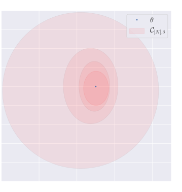
Figure 1: The model estimation procedure, running on the obstacle avoidance problem of Section 6. The confidence region $C_{N,\delta}$ shrinks with the number of samples $N$.

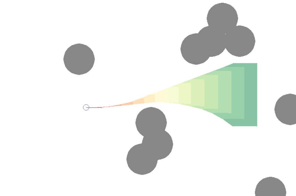
Figure 2: The state prediction procedure running on the obstacle avoidance problem of Section 6. At each time step (red to green), we bound the set of reachable states under model uncertainty (2)

Algorithm 1 Robust Estimation, Prediction and Control

  Input: confidence level $\delta$, structure $(A,\phi)$, reward $R$, $\mathcal{D}_{[0]}\leftarrow\emptyset,\,\mathbf{a}_{1}\leftarrow\emptyset$

  for $N=0,1,2,\dots$ do

     $\mathcal{C}_{N,\delta}\leftarrow$Model Estimation$(\mathcal{D}_{N})$. (9)

     for each planning step $k\in\{N,\dots,N+K\}=N+[K]$ do

        $[\underline{x}_{k+1},\overline{x}_{k+1}]\leftarrow$ Interval Prediction($\mathcal{C}_{N,\delta},\mathbf{a}_{k}b$) for each action $b\in\mathcal{A}$. (11)

        $\mathbf{a}_{k+1}$ $\leftarrow$Pessimistic Planning$(\underline{R_{k+1}}([\underline{x}_{k+1},\overline{x}_{k+1}]))$. (13)

     end for

     Execute the recommended control $u_{N+1}$, and add the transition $(x_{N+1},y_{N+1},u_{N+1})$ to $\mathcal{D}_{[N+1]}$.

  end for

1.1 Related Work

The control of uncertain systems is a long-standing problem, to which a vast body of literature is dedicated. Existing work is mostly concerned with the problem of stabilisation around a fixed reference state or trajectory, including approaches such as $\mathcal{H}_{\infty}$ control [7], sliding-mode control [32] or system-level synthesis [11, 12]. This paper fits in the popular MPC framework, for which adaptive data-driven schemes have been developed to deal with model uncertainty [38, 41, 5], but lack guarantees. The family of tube-MPC algorithms seeks to derive theoretical guarantees of robust constraint satisfaction: the state $x$ is constrained in a safe region $\mathbb{X}$ around the origin, often chosen convex [17, 4, 6, 42, 30, 22, 31, 28]. Yet, many tasks cannot be framed as stabilisation problems (e.g. obstacle avoidance) and are better addressed with the minimax control objective, which allows more flexible goal formulations. Minimax control has mostly been studied in two particular instances.

Finite states

Minimax control of finite Markov Decision Processes with uncertain parameters was studied in [21, 34, 44], who showed that the main results of Dynamic Programming can be extended to their robust counterparts only when the dynamics ambiguity set verifies a certain rectangularity property. Since we consider continuous states, these methods do not apply.

Linear dynamics and quadratic costs

Several approaches have been proposed for cumulative regret minimisation in the LQ problem. In the Optimism in the Face of Uncertainty paradigm, the best possible dynamics within a high-confidence region is selected under a controllability constraint, to compute the corresponding optimal control in closed-form by solving a Riccati equation. The results of [1, 20, 16] show that this procedure achieves a $\widetilde{\mathcal{O}}\left(N^{1/2}\right)$ regret. Posterior sampling algorithms [35, 3] select candidate dynamics randomly instead, and obtain the same result. Other works use noise injection for exploration such as [11, 12]. However, neither optimism nor random exploration fit a critical setting, where ensuring safety requires instead to consider pessimistic outcomes. The work of Dean et al. [11] is close to our setting: after an offline estimation phase, they estimate a suboptimality between a minimax controller and the optimal performance. Our work differs in that it addresses a generic shape cost. Another work of interest is [37] where worst-case generic costs are considered. However, they assume the knowledge of the dynamics, and their rollout-based solution only produces inner-approximations and does not yield any guarantee. In this paper, interval prediction is used to produce oversets, while a near-optimal control is found using a tree-based planning procedure.

2 Model Estimation

To derive a confidence region (2) for $\theta$, the functional relationship $A(\theta)$ must be specified.

Assumption 1 (Structure).

There exists a known feature tensor $\phi\in\mathbb{R}^{d\times p\times p}$ such that for all $\theta\in\Theta$,

$$A(\theta)=A+\sum_{i=1}^{d}\theta_{i}\phi_{i},$$ (5)

where $A,\phi_{1},\dots,\phi_{d}\in\mathbb{R}^{p\times p}$ are known. For all $n$, we denote $\Phi_{n}=[\phi_{1}x_{n}\dots\phi_{d}x_{n}]\in\mathbb{R}^{p\times d}$. We also assume to know a bound $S$ such that $\theta\in[-S,S]^{d}$.

We slightly abuse notations and include additional known terms in the measurement signal $y(t)=\dot{x}(t)+C\nu(t)-Ax(t)-Bu(t),$ to obtain a linear regression system $y_{n}=\Phi_{n}\theta+\eta_{n}.$

Regularised least square

To derive an estimate on $\theta$, we consider the $L_{2}$-regularised regression problem with weights $\Sigma_{p}\in\mathbb{R}^{p\times p}$ and $\lambda\in\mathbb{R}^{+}_{*}$:

$$\min_{\theta\in\mathbb{R}^{d}}\sum_{n=1}^{N}\|y_{n}-\Phi_{n}\theta\|_{\Sigma_{p}^{-1}}^{2}+\lambda\|\theta\|^{2}.~{}(6)$$

Proposition 1 (Regularised solution).

The solution to (2) is

$$\theta_{N,\lambda}=G_{N,\lambda}^{-1}\sum_{n=1}^{N}\Phi_{n}^{\mathsf{\scriptscriptstyle T}}\Sigma_{p}^{-1}y_{n},\qquad\text{where }\quad G_{N,\lambda}=\sum_{n=1}^{N}\Phi_{n}^{\mathsf{\scriptscriptstyle T}}\Sigma_{p}^{-1}\Phi_{n}+\lambda I_{d}\in\mathbb{R}^{d\times d}.$$ (7)

Substituting $y_{n}$ into (7) yields the regression error: $\theta_{N,\lambda}-\theta=G_{N,\lambda}^{-1}\sum_{n=1}^{N}\Phi_{n}^{\mathsf{\scriptscriptstyle T}}\Sigma_{p}^{-1}\eta_{n}-\lambda G_{N,\lambda}^{-1}\theta.$ To bound this error, we need the noise $\eta_{n}$ to concentrate.

Assumption 2 (Noise Model).

We assume that

1. at each time $t\geq 0$, the combined noise $\eta(t)$ is an independent sub-Gaussian noise with covariance proxy $\Sigma_{p}\in\mathbb{R}^{p\times p}$:

   $$\forall u\in\mathbb{R}^{p},\;\operatorname*{\mathbb{E}}\left[\exp{\left(u^{\mathsf{\scriptscriptstyle T}}\eta(t)\right)}\right]\leq\exp{\left(\frac{1}{2}u^{\mathsf{\scriptscriptstyle T}}\Sigma_{p}u\right)};$$

2. at each time $t\geq 0$, the disturbance $\omega(t)$ is enclosed by known bounds $\underline{\omega}(t)\leq\omega(t)\leq\overline{\omega}(t)$, whose amplitude verifies $\sum_{n=0}^{\infty}\gamma^{n}C_{\omega}(t_{n})<\infty$, where

   $$C_{\omega}(t)\stackrel{{\scriptstyle def}}{{=}}\sup_{\tau\in[0,t]}\|\overline{\omega}(\tau)-\underline{\omega}(\tau)\|_{2}.$$

Theorem 1 (Confidence ellipsoid, a matricial version of Abbasi-Yadkori et al. 2).

Under 2, it holds with probability at least $1-\delta$ that

$$\|\theta_{N,\lambda}-\theta\|_{G_{N,\lambda}}\leq\beta_{N}(\delta),\quad\text{with}\quad\beta_{N}(\delta)\stackrel{{\scriptstyle def}}{{=}}\sqrt{2\ln\left(\frac{\det(G_{N,\lambda})^{1/2}}{\delta\det(\lambda I_{d})^{1/2}}\right)}+(\lambda d)^{1/2}S.$$ (8)

We convert this confidence ellipsoid $\mathcal{C}_{N,\delta}$ from (8) into a polytope for $A(\theta)$. For simplicity, we present here a simple but coarse strategy: bound the ellipsoid by its enclosing axis-aligned hypercube:

$$A(\theta)\in\left\{A_{N}+\sum_{i=1}^{2^{d}}\alpha_{i}\Delta A_{N,i}:\alpha\geq 0,\sum_{i=1}^{2^{d}}\alpha_{i}=1\right\}$$ (9)

where $A_{N}=A(\theta_{N,\lambda}),\;h_{i}\in\{-1,1\}^{d},\;\Delta A_{N,i}={h_{i}}\sqrt{\frac{\beta_{N}(\delta)}{\lambda_{\max}(G_{N,\lambda})}}$. A tighter polytope derivation is presented in the Supplementary Material.

3 State Prediction

A simple solution to (4) is proposed in [14], where, given bounds $\underline{A}\leq A(\theta)\leq\overline{A}$ from $\mathcal{C}_{N,\delta}$ they use matrix interval arithmetic to derive the predictor:

Proposition 2 (Simple predictor of Efimov et al. 14).

Assuming that (2) is satisfied for the system (1), then the interval predictor following $\underline{x}(t_{N})=\overline{x}(t_{N})={x}(t_{N})$ and:

$$\dot{\underline{x}}(t)=\underline{A}^{+}\underline{x}^{+}(t)-\overline{A}^{+}\underline{x}^{-}(t)-\underline{A}^{-}\overline{x}^{+}(t)+\overline{A}^{-}\overline{x}^{-}(t)+Bu(t)+D^{+}\underline{\omega}(t)-D^{-}\overline{\omega}(t),$$ (10)

$$\dot{\overline{x}}(t)=\overline{A}^{+}\overline{x}^{+}(t)-\underline{A}^{+}\overline{x}^{-}(t)-\overline{A}^{-}\underline{x}^{+}(t)+\underline{A}^{-}\underline{x}^{-}(t)+Bu(t)+D^{+}\overline{\omega}(t)-D^{-}\underline{\omega}(t),$$

ensures the inclusion property (4) with confidence level $\delta$.

However, Leurent et al. [27] showed that this predictor can have unstable dynamics, even for stable systems, which causes a fast build-up of uncertainty. They proposed an enhanced predictor which exploits the polytopic structure (9) to produce more stable predictions, at the price of a requirement:

Assumption 3.

There exists an orthogonal matrix $Z\in\mathbb{R}^{p\times p}$ such that $Z^{\mathsf{\scriptscriptstyle T}}A_{N}Z$ is Metzler.

In practice, this assumption is often verified: it is for instance the case whenever $A_{N}$ is diagonalisable. The similarity transformation of [15] provides a method to compute such $Z$ when the system is observable. To simplify the notation, we will further assume that $Z=I_{p}$. Denote $\Delta A_{+}=\sum_{i=1}^{2^{d}}\Delta A_{N,i}^{+},\;\Delta A_{-}=\sum_{i=1}^{2^{d}}\Delta A_{N,i}^{-}$.

Proposition 3 (Enhanced predictor of Leurent et al. 27).

Assuming that (9) and 3 are satisfied for the system (1), then the interval predictor following $\underline{x}(t_{N})=\overline{x}(t_{N})={x}(t_{N})$ and:

$$\dot{\underline{x}}(t) = A_{N}\underline{x}(t)-\Delta A_{+}\underline{x}^{-}(t)-\Delta A_{-}\overline{x}^{+}(t)+Bu(t)+D^{+}\underline{\omega}(t)-D^{-}\overline{\omega}(t),$$ (11)

$$\dot{\overline{x}}(t) = A_{N}\overline{x}(t)+\Delta A_{+}\overline{x}^{+}(t)+\Delta A_{-}\underline{x}^{-}(t)+Bu(t)+D^{+}\overline{\omega}(t)-D^{-}\underline{\omega}(t),$$

ensures the inclusion property (4) with confidence level $\delta$.

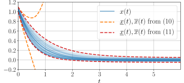
Figure 3: Comparison of (10) and (11) for a simple system $\dot{x}(t)=-\theta x(t)+\omega(t)$, with $\theta\in[1,2]$ and $\omega(t)\in[-0.05,0.05]$.

Figure 3 compares the performance of the predictors (10) and (11) in a simple example. It suggests to always prefer (11) whenever 3 is verified, and only fallback to (10) as a last resort.

4 Robust Control

To evaluate the robust objective $V^{r}$ (3), we approximate it thanks to the interval prediction $[\underline{x}(t),\overline{x}(t)]$.

Definition 1 (Surrogate objective).

Let $\underline{x}_{n}(\mathbf{u}),\overline{x}_{n}(\mathbf{u})$ following the dynamics defined in (11) and

$$\hat{V}^{r}(\mathbf{u})\stackrel{{\scriptstyle def}}{{=}}\sum_{n=N+1}^{\infty}\gamma^{n}\underline{R}_{n}(\mathbf{u})\quad\text{where}\quad\underline{R}_{n}(\mathbf{u})\stackrel{{\scriptstyle def}}{{=}}\min_{x\in[\underline{x}_{n}(\mathbf{u}),\overline{x}_{n}(\mathbf{u})]}R(x).$$ (12)

Such a substitution makes this pessimistic reward $\underline{R_{n}}$ not Markovian, since the worst case is assessed over the whole past trajectory.

Theorem 2 (Lower bound).

The surrogate objective (12) is a lower bound of the objective (3).

$$\hat{V}^{r}(\mathbf{u})\leq V^{r}(\mathbf{u})\leq V(\mathbf{u})$$

Consequently, since all our approximations are conservative, if we manage to find a control sequence such that no “bad event” (e.g. a collision) happens according to the surrogate objective $\hat{V}^{r}$, they are guaranteed not to happen either when the controls are executed on the true system.

To maximise $\hat{V}^{r}$, we cannot use DP algorithms since the state space is continuous and the pessimistic rewards are non-Markovian. Rather, we turn to tree-based planning algorithms, which optimise a sequence of actions based on the corresponding sequence of rewards, without requiring Markovity nor state enumeration. In particular, we consider the Optimistic Planning of Deterministic Systems (OPD) algorithm [19] tailored for the case when the relationship between actions and rewards is deterministic. Indeed, the stochasticity of the disturbances and measurements is encased in $\hat{V}^{r}$: given the observations up to time $N$ both the predictor dynamics (11) and the pessimistic rewards in (12) are deterministic. At each planning iteration $k\in[K]$, OPD progressively builds a tree $\mathcal{T}_{k+1}$ by forming upper-bounds $B_{a}(k)$ over the value of sequences of actions $a$, and expanding the leaf $a_{k}$ with highest upper-bound:

$$a_{k}=\operatorname*{arg\,max}_{a\in\mathcal{L}_{k}}B_{a}(k),\quad B_{a}(k)=\sum_{n=0}^{h(a)-1}\underline{R}_{n}(a)+\frac{\gamma^{h(a)}}{1-\gamma}$$ (13)

where $\mathcal{L}_{k}$ is the set of leaves of $\mathcal{T}_{k}$, $h(a)$ is the length of the sequence $a$, and $\underline{R}_{n}(a)$ the pessimistic reward (12) obtained at time $n$ by following the controls $u_{n}=\pi_{a_{n}}(x_{n})$.

Lemma 1 (Planning performance of Hren & Munos 19).

The suboptimality of the OPD algorithm (13) applied to the surrogate objective (12) after $K$ planning iterations is:

$$\hat{V}^{r}(a_{\star})-\hat{V}^{r}({a_{K}})=\mathcal{O}\left(K^{-\frac{\log 1/\gamma}{\log\kappa}}\right);$$

where $\kappa\stackrel{{\scriptstyle def}}{{=}}\limsup_{h\rightarrow\infty}\left|\left\{a\in A^{h}:\hat{V}^{r}(a)\geq\hat{V}^{r}(a^{\star})-\frac{\gamma^{h+1}}{1-\gamma}\right\}\right|^{1/h}$ is a problem-dependent measure of the proportion of near-optimal paths.

Hence, by using enough computational budget $K$ for planning we can get as close as we want to the optimal surrogate value $\hat{V}^{r}(a^{\star})$, at a polynomial rate. Unfortunately, there exists a gap between $\hat{V}^{r}$ and the true robust objective $V^{r}$, which stems from three approximations: (i) the true reachable set was approximated by an enclosing interval in (4); (ii) the time-invariance of the dynamics uncertainty $A(\theta)\in\mathcal{C}_{N,\delta}$ was handled by the interval predictor (11) as if it were a time-varying uncertainty $A(\theta(t))\in\mathcal{C}_{N,\delta},\forall t$ ; and (iii) the lower-bound $\sum\min\leq\min\sum$ used to define the surrogate objective (12) is not tight. However, this gap can be bounded under additional assumptions.

Theorem 3 (Suboptimality bound).

Under two conditions:

1. a Lipschitz regularity assumption for the reward function $R$:

2. a stability condition: there exist $P>0,Q_{0}\in\mathbb{R}^{p\times p}$, $\rho>0$, and $N_{0}\in\mathbb{N}$ such that

   $$\forall N>N_{0},\quad\begin{bmatrix}A_{N}^{\mathsf{\scriptscriptstyle T}}P+PA_{N}+Q_{0}&P|D|\\ |D|^{\mathsf{\scriptscriptstyle T}}P&-\rho I_{r}\\ \end{bmatrix}<0;$$

we can bound the suboptimality of Algorithm 1 with planning budget $K$ as:

$$V(a_{\star})-\hat{V}^{r}(a_{K})\leq{\color[rgb]{1,0,0}\underbrace{\Delta_{\omega}}_{\begin{subarray}{c}\text{robustness to}\\ \text{disturbances}\end{subarray}}}+{\color[rgb]{0,0,1}\underbrace{\mathcal{O}\left(\frac{\beta_{N}(\delta)^{2}}{\lambda_{\min}(G_{N,\lambda})}\right)}_{\text{estimation error}}}+{\color[rgb]{0.0,0.42,0.24}\underbrace{\mathcal{O}\left(K^{-\frac{\log 1/\gamma}{\log\kappa}}\right)}_{\text{planning error}}}$$

with probability at least $1-\delta$, where $V(a)$ is the optimal expected return when executing an action $a\in\mathcal{A}$, $a_{\star}$ is an optimal action, and ${\color[rgb]{1,0,0}\Delta_{\omega}}$ is a constant which corresponds to an irreducible suboptimality suffered from being robust to instantaneous disturbances $\omega(t)$.

It is difficult to check the validity of the stability condition 2. since it applies to matrices $A_{N}$ produced by the algorithm rather than to the system parameters. A stronger but easier to check condition is that the polytope (9) at some iteration becomes included in a set where this property is uniformly satisfied. For instance, if the features are sufficiently excited, the estimation converges to a neighbourhood of the true dynamics $A(\theta)$. This also allows to further bound the input-dependent estimation error term.

Corollary 1 (Asymptotic near-optimality).

Under an additional persistent excitation (PE) assumption

$$\exists\underline{\phi},\overline{\phi}>0:\forall n\geq n_{0},\quad\underline{\phi}^{2}\leq\lambda_{\min}(\Phi_{n}^{\mathsf{\scriptscriptstyle T}}\Sigma_{p}^{-1}\Phi_{n})\leq\overline{\phi}^{2},$$ (14)

the stability condition 2. of Theorem 3 can be relaxed to apply to the true system: there exist $P,Q_{0},\rho$ such that

$$\begin{bmatrix}A(\theta)^{\mathsf{\scriptscriptstyle T}}P+PA(\theta)+Q_{0}&P|D|\\ |D|^{\mathsf{\scriptscriptstyle T}}P&-\rho I_{r}\\ \end{bmatrix}<0;$$

and the suboptimality bound takes the more explicit form

$$V(a_{\star})-\hat{V}^{r}(a_{K})\leq{\color[rgb]{1,0,0}{\Delta_{\omega}}}+{\color[rgb]{0,0,1}{\mathcal{O}\left(\frac{\log\left(N^{d/2}/\delta\right)}{N}\right)}}+{\color[rgb]{0.0,0.42,0.24}{\mathcal{O}\left(K^{-\frac{\log 1/\gamma}{\log\kappa}}\right)}}$$

which ensures asymptotic near-optimality when $N\to\infty$ and $K\to\infty$.

5 Multi-model Selection

The procedure we developed in Sections 2, 3 and 4 relies on strong modelling assumptions, such as the linear dynamics (1) and 1. But what if they are wrong?

Model adequacy

One of the major benefits of using the family of linear models, compared to richer model classes, is that they provide strict conditions allowing to quantify the adequacy of the modelling assumptions to the observations. Given $N-1$ observations, Section 2 provides a polytopic confidence region (9) that contains $A(\theta)$ with probability at least $1-\delta$. Since the dynamics are linear, we can propagate this confidence region to the next observation: $y_{N}$ must belong to the Minkowski sum of a polytope representing model uncertainty $\mathcal{P}(A_{0}x_{N}+Bu_{N},\Delta A_{1}x_{N},\dots,\Delta A_{2^{d}}x_{N})$ and a polytope $\mathcal{P}(0_{p},\underline{\eta},\overline{\eta})$ bounding the disturbance and measurement noises. Delos & Teissandier [13] provide a way to test this membership in polynomial time using linear programming. Whenever it is not verified, we can confidently reject the $(A,\phi)$-modelling 1. This enables us to consider a rich set of potential features $\left((A^{1},\phi^{1}),\dots,(A^{M},\phi^{M})\right)$ rather than relying on a single assumption, and only retain those that are consistent with the observations so far. Then, every remaining hypothesis must be considered during planning.

Robust selection

We temporarily ignore the parametric uncertainty on $\theta$ to simply consider several candidate dynamics models, which all correspond to different modelling assumptions. We also restrict to deterministic dynamics, which is the case of (11).

Assumption 4 (Multi-model ambiguity).

The dynamics $f$ lie in a finite set of candidates $(f^{m})_{m\in[M]}$.

We adapt our planning algorithm to balance these concurrent hypotheses in a robust fashion, i.e. maximise a robust objective with discrete ambiguity:

$$V^{r}=\sup_{a\in\mathcal{A}^{\mathbb{N}}}\min_{m\in[M]}\sum_{n=N+1}^{\infty}\gamma^{n}R_{n}^{m},$$ (15)

where $R_{n}^{m}$ is the reward obtained by following the action sequence $a$ up to step $n$ under the dynamics $f^{m}$. This objective could be optimised in the same way as in Section 4, but this would result in a coarse and lossy approximation. Instead, we exploit the finite uncertainty structure of 4 to asymptotically recover the true $V^{r}$ by modifying the OPD algorithm in the following way:

Definition 2 (Robust UCB).

We replace the upper-bound (13) on sequence values in OPD by:

$$B_{a}^{r}(k)\stackrel{{\scriptstyle def}}{{=}}\min_{m\in[M]}\sum_{n=0}^{h-1}\gamma^{n}R_{n}^{m}+\frac{\gamma^{h}}{1-\gamma}.$$ (16)

Note that it is not equivalent to solving each control problem independently and following the action with highest worst-case value, as we show in the Supplementary Material. We analyse the sample complexity of the corresponding robust planning algorithm.

Proposition 4 (Robust planning performance).

The robust version of OPD (16) enjoys the same regret bound as OPD in Lemma 1, with respect to the multi-model objective (15).

This result is of independent interest: the solution of a robust objective (15) with discrete ambiguity $f\in\{f^{m}\}_{m\in[M]}$ can be recovered exactly, asymptotically when the planning budget $K$ goes to infinity, which Robust DP algorithms do not allow. This also contrasts with the results obtained in Section 4 for the robust objective (3) with continuous ambiguity $A(\theta)\in\mathcal{C}_{N,\delta}$, for which OPD only recovers the surrogate approximation $\hat{V}^{r}$, as discussed in Theorem 3. Note that here the regret depends on the number $K$ of node expansions, but each expansion now requires $M$ times more simulations than in the single-model setting. Finally, the two approaches of Sections 4 and 5 can be merged by using the pessimistic reward (12) in (16).

6 Experiments

Videos and code are available at https://eleurent.github.io/robust-beyond-quadratic/.

Obstacle avoidance with unknown friction

We first consider a simple illustrative example, shown in Figure 2: the control of a 2D system moving by means of a force $(u_{x},u_{y})$ in an medium with anisotropic linear friction with unknown coefficients $(\theta_{x},\theta_{y})$. The reward encodes the task of navigating to reach a goal state $x_{g}$ while avoiding collisions with obstacles: $R(x)=\delta(x)/(1+\|x-x_{g}\|_{2})$ where $\delta(x)$ is $0$ whenever $x$ collides with an obstacle, $1$ otherwise. The actions $\mathcal{A}$ are constant controls in the up, down, left and right directions. For the reasons mentioned above, no robust baseline applies to our setting. We compare Algorithm 1 to the non-robust adaptive control approach that plans with the estimated dynamics $\theta_{N,\lambda}$, and thus enjoys the same prior knowledge of dynamics structure and reward. This highlights the benefits of the robust formulation solely rather than stemming from algorithm design. We show in Figure 6(a) the results of 100 simulations of a single episode: the robust agent performs worse than the nominal agent on average, but manages to ensure safety while the nominal agent collides with obstacles in $4\%$ of simulations. We also compare to a standard model-free approach, DQN, which does not benefit from the prior knowledge on the system dynamics, and is instead trained over multiple episodes. The reported performance is that of the final policy obtained after training for 3000 episodes, during which $897\pm 64$ collisions occurred ($29.9\pm 2.1$%). We study the evolution of the suboptimality $V(x_{N})-\sum_{n>N}\gamma^{n-N}R(x_{n})$ with respect to the number of samples $N$, by comparing the empirical returns from a state $x_{N}$ to the value $V(x_{N})$ that the agent would get by acting optimally from $x_{N}$ with knowledge of the dynamics. Although the assumptions of Theorem 3 are not satisfied (e.g. non-smooth reward), the mean suboptimality of the robust agent, shown in Figure 5, still decreases polynomially with $N$: Algorithm 1 gets more efficient as it is more confident while ensuring safety at all times. In comparison, the nominal agent enjoys a smaller suboptimality on average, but higher in the worst-case.

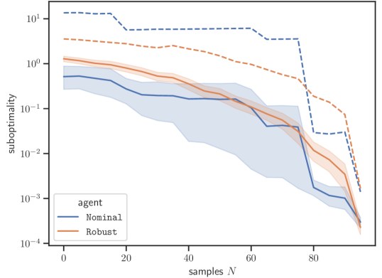
Figure 4: The mean (solid), $95\%$ CI for the mean (shaded) and maximum (dashed) suboptimality with respect to $N$.

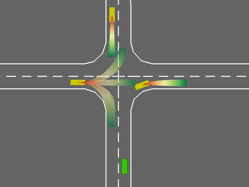
Figure 5: The intersection crossing task. Trajectory intervals show behavioural uncertainty for each vehicle, with a multi-model assumption over their route.

Table 1: Frequency of collision, minimum and average return achieved on a single episode, repeated with 100 random seeds. In both tasks, the robust agent performs worse than the nominal agent on average, but manages to ensure safety and attains a better worst-case performance.

Performance	failures	min	avg $\pm$ std
Oracle	0%	11.6	$14.2\pm 1.3$
Nominal	4%	2.8	$\mathbf{13.8}\pm 2.0$
Algorithm 1	0%	10.4	$13.0\pm 1.5$
DQN (trained)	6%	1.7	$12.3\pm 2.5$

(a) Performances on the obstacle task

Performance	failures	min	avg $\pm$ std
Oracle	0%	6.9	$7.4\pm 0.5$
Nominal 1	4%	5.2	$\mathbf{7.3}\pm 1.5$
Nominal 2	33%	3.5	$6.4\pm 0.3$
Algorithm 1	0%	6.8	$7.1\pm 0.3$
DQN (trained)	3%	5.4	$6.3\pm 0.6$

(b) Performances on the driving task

Motion planning for an autonomous vehicle   We consider the highway-env environment [25] for simulated driving decision problems. An autonomous vehicle with state $\chi_{0}\in\mathbb{R}^{4}$ is approaching an intersection among $V$ other vehicles with states $\chi_{i}\in\mathbb{R}^{4}$, resulting in a joint traffic state $x=[\chi_{0},\dots,\chi_{V}]^{\top}\in\mathbb{R}^{4V+4}$. These vehicles follow parametrized behaviours $\dot{\chi}_{i}=f_{i}(x,\theta_{i})$ with unknown parameters $\theta_{i}\in\mathbb{R}^{5}$. We appreciate a first advantage of the structure imposed in 1: the uncertainty space of $\theta$ is $\mathbb{R}^{5V}$. In comparison, the traditional LQ setting where the whole state matrix $A$ is estimated would have resulted in a much larger parameter space $\theta\in\mathbb{R}^{16V^{2}}$. The system dynamics $f$, which describes the interactions between vehicles, can only be expressed in the form of 1 given the knowledge of the desired route for each vehicle, with features $\phi$ expressing deviations to the centerline of the followed lane. Since these intentions are unknown to the agent, we adopt the multi-model perspective of Section 5 and consider one model per possible route for every observed vehicle before an intersection. In Figure 6(b), we compare Algorithm 1 to a nominal agent planning with two different modelling assumptions: Nominal 1 has access to the true followed route for each vehicle, while Nominal 2 does not and picks the model with minimal prediction error. Again we also compare to a DQN baseline trained over 3000 episodes, causing $1058\pm 113$ collisions while training ($35\pm 4\%$). As before, the robust agent has a higher worst-case performance and avoids collisions at all times, at the price of a decreased average performance..

Conclusion

We present a framework for the robust estimation, prediction and control of a partially known linear system with generic costs. Leveraging tools from linear regression, interval prediction, and tree-based planning, we guarantee the predicted performance and provide a suboptimality bound. The method applicability is further improved by a multi-model extension and demonstrated on two simulations.

Broader Impact

The motivation behind this work is to enable the development of Reinforcement Learning solutions for industrial applications, when it has been mainly limited to simulated games so far. In particular, many industries already rely on non-adaptive control systems and could benefit from an increased efficiency, including Oil and Gas, robotics for industrial automation, Data Center cooling, etc. But more often than not, safety-critical constraints proscribe the use of exploration, and industrials are reluctant to turn to learning-based methods that lack accountability. This work addresses these concerns by focusing on risk-averse decisions and by providing worst-case guarantees. Note however that these guarantees are only as good as the validity of the underlying hypotheses, and 1 in particular should be submitted to a comprehensive validation procedure; otherwise, decisions formed on a wrong basis could easily lead to dramatic consequences in such critical settings. Beyond industrial perspectives, this work could be of general interest for risk-averse decision-making. For instance, parametrized epidemiological models have been used to represent the propagation of Covid-19 and study the impact of lockdown policies. These model parameters are estimated from observational data and corresponding confidence intervals are often available, but rarely used in the decision-making loop. In contrast, our approach would enable evaluating and optimising the worst-case outcome of such public policies.

Supplementary Material

Outline

In Appendix A, we provide a proof for every novel result introduced in this paper. Appendix B provides additional details on our experiments. Appendix C gives a better method of conversion from ellipsoid to polytope than that of (9). Finally, Appendix D highlights the fact that robustness cannot be recovered by aggregating independent solutions to many optimal control problem.

Appendix A Proofs

A.1 Proof of Proposition 1

Proof.

We differentiate $J(\theta)=\sum_{n=1}^{N}\|y_{n}-\Phi_{n}\theta\|_{\Sigma_{p}^{-1}}^{2}+\lambda\|\theta\|^{2}$ as in (2) with respect to $\theta$:

$$\nabla_{\theta}J(\theta) =\sum_{n=1}^{N}\nabla_{\theta}(y_{n}-\Phi_{n}\theta)^{\mathsf{\scriptscriptstyle T}}\Sigma_{p}^{-1}(y_{n}-\Phi_{n}\theta)+\nabla_{\theta}\lambda\|\theta\|^{2}$$

$$=-2\sum_{n=1}^{N}y_{n}^{\mathsf{\scriptscriptstyle T}}\Sigma_{p}^{-1}\Phi_{n}+2\sum_{n=1}^{N}\theta^{\mathsf{\scriptscriptstyle T}}(\Phi_{n}^{\mathsf{\scriptscriptstyle T}}\Sigma^{-1}\Phi_{n})+2\lambda\theta^{\mathsf{\scriptscriptstyle T}}$$

Hence,

$$\nabla_{\theta}J(\theta)=0\iff\left(\sum_{n=1}^{N}\Phi_{n}^{\mathsf{\scriptscriptstyle T}}\Sigma_{p}^{-1}\Phi_{n}+I_{d}\right)\theta=\sum_{n=1}^{N}y_{n}^{\mathsf{\scriptscriptstyle T}}\Sigma_{p}^{-1}\Phi_{n}$$

∎

A.2 Proof of Theorem 1

We start by showing a preliminary proposition:

Proposition 5 (Matrix version of Theorem 1 of Abbasi-Yadkori et al. 2).

Let $\{F_{n}\}_{n=0}$ be a filtration. Let $\{\eta_{n}\}_{n=1}^{\infty}$ be a $\mathbb{R}^{p}$-valued stochastic process such that $\eta_{n}$ is $F_{n}$-measurable and $\operatorname*{\mathbb{E}}\left[\eta_{n}\;\middle|\;F_{n-1}\right]$ is $\Sigma_{p}$-sub-Gaussian.

Let $\{\Phi_{n}\}_{n=1}^{\infty}$ be an $\mathbb{R}^{p\times d}$-valued stochastic process such that $\Phi_{n}$ is $F_{n}$-measurable. Assume that $G$ is a $d\times d$ positive definite matrix. For any $n\geq 0$, define:

$$\overline{G}_{n}=G+\sum_{s=1}^{n}\Phi_{s}^{\mathsf{\scriptscriptstyle T}}\Sigma_{p}^{-1}\Phi_{s}\in\mathbb{R}^{d\times d}\quad S_{n}=\sum_{s=1}^{n}\Phi_{s}^{\mathsf{\scriptscriptstyle T}}\Sigma_{p}^{-1}\eta_{s}\in\mathbb{R}^{d}.$$

Then, for any $\delta>0$, with probability at least $1-\delta$, for all $n\geq 0$,

$$\|S_{n}\|_{\overline{G}_{n}^{-1}}\leq\sqrt{2\ln\left(\frac{\det\left(\overline{G}_{n}\right)^{1/2}}{\delta\det(G)^{1/2}}\right)}.$$

Proof.

Let

$$G_{t}=\sum_{s=1}^{t}\Phi_{s}^{\mathsf{\scriptscriptstyle T}}\Sigma_{p}^{-1}\Phi_{s}\in\mathbb{R}^{d\times d}$$

And for any $z\in\mathbb{R}^{d}$,

$$M_{t}^{z}=\exp{\left(\langle z,S_{t}\rangle-\frac{1}{2}\|z\|_{G_{t}}\right)}$$

$$D_{t}^{z}=\exp{\left(\langle\Phi_{t}z,\eta_{t}\rangle_{\Sigma_{p}^{-1}}-\frac{1}{2}\|\Phi_{t}z\|_{\Sigma_{p}^{-1}}\right)}$$

Then,

$$M_{t}^{z} =\exp{\left(\sum_{s=1}^{t}z^{\mathsf{\scriptscriptstyle T}}\Phi_{s}^{\mathsf{\scriptscriptstyle T}}\Sigma_{p}^{-1}\eta_{s}-\frac{1}{2}(\Phi_{s}z)^{\mathsf{\scriptscriptstyle T}}\Sigma_{p}^{-1}(\Phi_{s}z)\right)}$$

$$=\prod_{s=1}^{t}D_{s}^{z}$$

and using the Sub-Gaussianity of $\eta_{t}$

$$\operatorname*{\mathbb{E}}\left[D_{t}^{z}\;\middle|\;F_{t-1}\right]={} \exp{\left(-\frac{1}{2}\|\Phi_{t}z\|_{\Sigma_{p}^{-1}}\right)}$$

$$\operatorname*{\mathbb{E}}\left[\exp{\left(\langle\Phi_{t}z,\eta_{t}\rangle_{\Sigma_{p}^{-1}}\right)}\;\middle|\;F_{t-1}\right]$$

$$\leq{} \exp{\left(-\frac{1}{2}\|\Phi_{t}z\|_{\Sigma_{p}^{-1}}\right)}$$

$$\exp{\left((z^{\mathsf{\scriptscriptstyle T}}\Phi_{t}^{\mathsf{\scriptscriptstyle T}}\Sigma_{p}^{-1})\Sigma_{p}(\Sigma_{p}^{-1}\Phi_{t}z)\right)}$$

$$=1$$

$$\operatorname*{\mathbb{E}}\left[M_{t}^{z}\;\middle|\;F_{t-1}\right]=\left(\prod_{s=1}^{t-1}D_{s}^{z}\right)\operatorname*{\mathbb{E}}\left[D_{t}^{z}\;\middle|\;F_{t-1}\right]\leq M_{t-1}^{z}$$

Showing that $(M_{t}^{z})_{t=1}^{\infty}$ is indeed a supermartingale and in fact $\operatorname*{\mathbb{E}}[M_{t}^{z}]\leq 1$. It then follows by Doob’s upcrossing lemma for supermartingale that $M_{\infty}^{z}=\lim_{t\to\infty}M_{t}^{z}$ is almost surely well-defined, and so is $M_{\tau}^{z}$ for any random stopping time $\tau$.

Next, we consider the stopped martingale $M_{\min(\tau,t)}^{z}$. Since $(M_{t}^{z})_{t=1}^{\infty}$ is a non-negative supermartingale and $\tau$ is a random stopping time, we deduce by Doob’s decomposition that

$$\operatorname*{\mathbb{E}}[M_{\min(\tau,t)}^{z}] =\operatorname*{\mathbb{E}}[M_{0}^{z}]+\operatorname*{\mathbb{E}}[\sum_{s=0}^{t-1}(M_{s+1}^{z}-M_{s}^{z})\mathbb{I}\{\tau>s\}]$$

$$\leq 1+\operatorname*{\mathbb{E}}[\sum_{s=0}^{t-1}\operatorname*{\mathbb{E}}[M_{s+1}^{z}-M_{s}^{z}|F_{s}]\mathbb{I}\{\tau>s\}]$$

$$\leq 1$$

Finally, an application of Fatou’s lemma show that $\operatorname*{\mathbb{E}}[M_{\tau}^{z}]=\operatorname*{\mathbb{E}}[\liminf_{t\to\infty}M_{\min(\tau,t)}^{z}]\leq\liminf_{t\to\infty}\operatorname*{\mathbb{E}}[M_{\min(\tau,t)}^{z}]\leq 1.$

This results allows to apply a result from [36]:

Lemma 2 (Theorem 14.7 of [36]).

If $Z$ is a random vector and $B$ is a symmetric positive definite matrix such that

$$\forall\gamma\in\mathbb{R}^{d},\ln\operatorname*{\mathbb{E}}\exp\left(\gamma^{\mathsf{\scriptscriptstyle T}}Z-\frac{1}{2}\gamma^{\mathsf{\scriptscriptstyle T}}B\gamma\right)\leq 0,$$

then for any positive definite non-random matrix C, it holds

$$\operatorname*{\mathbb{E}}\left[\sqrt{\frac{\det(C)}{\det(B+C)}}\exp\left(\frac{1}{2}\|Z\|^{2}_{(B+C)^{-1}}\right)\right]\leq 1.$$

In particular, by Markov inequality, for all $\delta\in(0,1)$,

$$\mathbb{P}\left(\|Z\|_{(B+C)^{-1}}\geq\sqrt{2\ln\left(\frac{\det\left((B+C)^{1/2}\right)}{\delta\det(C)^{1/2}}\right)}\right)\leq\delta.$$

Here, by using $Z=\sum_{s=1}^{t}\Phi_{s}\Sigma_{p}^{-1}\eta_{s}$, $B=G_{t}$, $C=G$,

$$\mathbb{P}\left(\|S_{t}\|_{(G_{t}+G)^{-1}}\geq\sqrt{2\ln\left(\frac{\det(G_{t}+G)^{1/2}}{\delta\det(G)^{1/2}}\right)}\right)\leq\delta$$

∎

Having shown this preliminary result, we move on to the proof of Theorem 1.

Proof.

For all $x\in\mathbb{R}^{d}$, (7) gives:

$$x^{\mathsf{\scriptscriptstyle T}}\theta_{N,\lambda}-x^{\mathsf{\scriptscriptstyle T}}\theta =x^{\mathsf{\scriptscriptstyle T}}G_{N,\lambda}^{-1}\sum_{n=1}^{N}\Phi_{n}^{\mathsf{\scriptscriptstyle T}}\Sigma_{p}^{-1}\eta_{n}-\lambda x^{\mathsf{\scriptscriptstyle T}}G_{N,\lambda}^{-1}\theta$$

$$=\langle x,\sum_{n=1}^{N}\Phi_{n}^{\mathsf{\scriptscriptstyle T}}\Sigma_{p}^{-1}\eta_{n}\rangle_{G_{N,\lambda}^{-1}}-\lambda\langle x,\theta\rangle_{G_{N,\lambda}^{-1}}$$

Using the Cauchy-Schwartz inequality, we get:

$$|x^{\mathsf{\scriptscriptstyle T}}\theta_{N,\lambda}-x^{\mathsf{\scriptscriptstyle T}}\theta|\leq{} \|x\|_{G_{N,\lambda}^{-1}}\left(\left\|\sum_{n=1}^{N}\Phi_{n}^{\mathsf{\scriptscriptstyle T}}\Sigma_{p}^{-1}\eta_{n}\right\|_{G_{N,\lambda}^{-1}}\right.$$

$$+\left.\lambda\|\theta\|_{G_{N,\lambda}^{-1}}\right)$$

In particular, for $x=G_{N,\lambda}(\theta_{N,\lambda}-\theta)$, we get after simplifying with $\|\theta_{N,\lambda}-\theta\|_{G_{N,\lambda}}$:

$$\|\theta_{N,\lambda}-\theta\|_{G_{N,\lambda}} \leq\left\|\sum_{n=1}^{N}\Phi_{n}^{\mathsf{\scriptscriptstyle T}}\Sigma_{p}^{-1}\eta_{n}\right\|_{G_{N,\lambda}^{-1}}+\lambda\|\theta\|_{G_{N,\lambda}^{-1}}$$

By applying Proposition 5 with $G=\lambda I_{d}$, we obtain that with probability at least $1-\delta$,

$$\|\theta_{N,\lambda}-\theta\|_{G_{N,\lambda}} \leq\sqrt{2\ln\left(\frac{\det(G_{N,\lambda})^{1/2}}{\delta\det(\lambda I_{d})^{1/2}}\right)}+\lambda\|\theta\|_{G_{N,\lambda}^{-1}}$$

And since $\|\theta\|_{G_{N,\lambda}^{-1}}^{2}\leq 1/\lambda_{\min}(G_{N,\lambda})\|\theta\|_{2}^{2}\leq 1/\lambda\|\theta\|_{2}^{2}$ and $\|\theta\|_{2}^{2}\leq d\|\theta\|_{\infty}^{2}\leq dS^{2}$,

$$\|\theta_{N,\lambda}-\theta\|_{G_{N,\lambda}} \leq\sqrt{2\ln\left(\frac{\det(G_{N,\lambda})^{1/2}}{\delta\det(\lambda I_{d})^{1/2}}\right)}+(\lambda d)^{1/2}S$$

∎

A.3 Proof of Theorem 2

Proof.

The predictor designed in Section 3 verifies the inclusion property (4). Thus, for sequence of controls $\mathbf{u}$, any dynamics $A(\theta)\in C_{N,\delta}$, and disturbances $\underline{\omega}\leq\omega\leq\overline{\omega}$, the corresponding state at time $t_{n}$ is bounded by $\underline{x}_{n}\leq x_{n}\leq\overline{x}_{n}$, which implies that $R(x_{n})\geq\min_{x\in[\underline{x}_{n}(\mathbf{u}),\overline{x}_{n}(\mathbf{u})]}R(x)=\underline{R}_{n}(\mathbf{u})$.

Thus, by taking the min over $C_{N,\delta}$ and $[\underline{\omega},\overline{\omega}]$, we also have for any sequence of controls $\mathbf{u}$:

$$V^{r}(\mathbf{u}) =\min_{\begin{subarray}{c}A(\theta)\in C_{N,\delta}\\ \underline{\omega}\leq\omega\leq\overline{\omega}\end{subarray}}\sum_{n=N+1}^{\infty}\gamma^{n}R(x_{n})$$

$$\geq\sum_{n=N+1}^{\infty}\gamma^{n}\underline{R}_{n}(\mathbf{u})$$

$$=\hat{V}^{r}(\mathbf{u})$$

And $V^{r}(\mathbf{u})\leq V(\mathbf{u})=\operatorname*{\mathbb{E}}_{\omega}\left[\sum_{n=N+1}^{\infty}\gamma^{n}R(x_{n})\right]$ by definition. ∎

A.4 Proof of Theorem 3

We first bound the model estimation error.

Lemma 3.

$$\|A(\theta)-A(\theta_{N,\lambda})\|_{F}=\mathcal{O}\left(\sqrt{{\frac{\beta_{N}(\delta)^{2}}{\lambda_{\min}(G_{N,\lambda})}}}\right)$$

Proof.

We have

$$\|\theta-\theta_{N,\lambda}\|_{G_{N,\lambda}}^{2}\geq\lambda_{\min}(G_{N,\lambda})\|\theta-\theta_{N,\lambda}\|_{2}^{2}$$

And (8) gives

$$\|\theta-\theta_{N,\lambda}\|_{G_{N,\lambda}}^{2}=\mathcal{O}(\beta_{N}(\delta)^{2})$$

Moreover, $A(\theta)$ belongs to a linear image of this $L^{2}$-ball. By writing a the $j^{th}$ column of a matrix $M$ as $M_{j}$, and its coefficient $i,j$ as $M_{i,j}$,

$$((A(\theta)-A(\theta_{N,\lambda}))^{\mathsf{\scriptscriptstyle T}}(A(\theta)-A(\theta_{N,\lambda})))_{i,j} =(\theta-\theta_{N,\lambda})^{\mathsf{\scriptscriptstyle T}}\phi_{i}^{\mathsf{\scriptscriptstyle T}}\phi_{j}(\theta-\theta_{N,\lambda})$$

$$\leq\lambda_{\max}(\phi_{i}^{\mathsf{\scriptscriptstyle T}}\phi_{j})\|\theta-\theta_{N,\lambda}\|_{2}^{2}$$

Thus, $\|A(\theta)-A(\theta_{N,\lambda})\|_{F}^{2}=\operatorname{Tr}{\left[(A(\theta)-A(\theta_{N,\lambda}))^{\mathsf{\scriptscriptstyle T}}(A(\theta)-A(\theta_{N,\lambda}))\right]}=\mathcal{O}\left({\frac{\beta_{N}(\delta)^{2}}{\lambda_{\min}(G_{N,\lambda})}}\right)$

∎

Then, we propagate this estimation error through the state prediction.

Lemma 4.

If there exist $P>0,Q_{0}\in\mathbb{R}^{p\times p}$, $\rho>0$ such that

$$\begin{bmatrix}A_{N}^{\mathsf{\scriptscriptstyle T}}P+PA_{N}+Q_{0}&P|D|\\ |D|^{\mathsf{\scriptscriptstyle T}}P&-\rho I_{r}\\ \end{bmatrix}<0,$$

then for all $t>t_{N}$,

$$\|\overline{x}(t)-\underline{x}(t)\|\leq\left(C_{0}+\mathcal{O}\left({\frac{\beta_{N}(\delta)}{\sqrt{\lambda_{\min}(G_{N,\lambda})}}}\right)\right)C_{\omega}(t),$$

where

$$C_{0}=\sqrt{\frac{2\rho\lambda_{\max}(P)}{\lambda_{\min}(P)\lambda_{\min}(Q_{0})}},$$

and

$$C_{\omega}(t)=\sup_{\tau\in[0,t]}\|\overline{\omega}(\tau)-\underline{\omega}(\tau)\|_{2}.$$

Proof.

Let $e=\overline{x}-\underline{x}$. (11) gives the dynamics

$$\dot{e}=A_{N}e+|\Delta A|(\overline{x}^{+}+\underline{x}^{-})+|D|(\overline{\omega}-\underline{\omega})$$

where recall that $|M|=M^{+}+M^{-}$ for any matrix $M\in\mathbb{R}^{p\times p}$.

We define the Lyapunov function $V=e^{\mathsf{\scriptscriptstyle T}}Pe$, which is non-negative definite provided that $P>0,$ and compute its derivative

$$\dot{V}={} X^{\mathsf{\scriptscriptstyle T}}\begin{bmatrix}A_{N}^{\mathsf{\scriptscriptstyle T}}P+PA_{N}+Q&P|D|&P|\Delta A|\\ |D|^{\mathsf{\scriptscriptstyle T}}P&-\rho I_{r}&0\\ |\Delta A|^{\mathsf{\scriptscriptstyle T}}P&0&-\alpha I_{p}\end{bmatrix}X$$

$$-e^{\mathsf{\scriptscriptstyle T}}Qe+\alpha|\underline{x}^{+}+\overline{x}^{-}|^{2}+\rho|\overline{\omega}-\underline{\omega}|^{2}$$

with $X=\begin{bmatrix}e&\overline{\omega}-\underline{\omega}&\underline{x}^{+}+\overline{x}^{-}\end{bmatrix}^{\mathsf{\scriptscriptstyle T}}$, for any $Q\in\mathbb{R}^{p\times p}$, $\rho,\alpha\in\mathbb{R}$ .

Moreover, it holds that $-\underline{x}^{+}-\overline{x}^{-}\leq e\leq\overline{x}^{+}+\underline{x}^{-}$, which implies $|\underline{x}^{+}+\overline{x}^{-}|\leq 2|e|$. Hence,

$$\dot{V}\leq{} X^{\mathsf{\scriptscriptstyle T}}\underbrace{\left[\begin{array}[]{cc|c}A_{N}^{\mathsf{\scriptscriptstyle T}}P+PA_{N}+Q+4\alpha I_{p}&P|D|&P|\Delta A|\\ |D|^{\mathsf{\scriptscriptstyle T}}P&-\rho I_{r}&0\\ \hline\cr|\Delta A|^{\mathsf{\scriptscriptstyle T}}P&0&-\alpha I_{p}\end{array}\right]}_{\Upsilon}X$$

$$-e^{\mathsf{\scriptscriptstyle T}}Qe+\rho\|\overline{\omega}-\underline{\omega}\|_{2}^{2}$$

Thus, if we had $\Upsilon\leq 0$, $Q>0$, $\rho>0$, then we would have

$$\dot{V}\leq-\mu V+\rho\|\overline{\omega}-\underline{\omega}\|_{2}^{2}$$

with $\mu=\frac{\lambda_{\min}(Q)}{\lambda_{\max}(P)}$. Since $V(t_{N})=0$, this further implies that for all $t>t_{N}$,

$$V(t)\leq\frac{\rho}{\mu}C_{\omega}^{2}(t)$$ (17)

We now examine the condition $\Upsilon\leq 0$. We resort to its Schur complement: given $\alpha>0$, $\Upsilon\leq 0$ if and only if $R\geq S$, where $S=\alpha^{-1}\begin{bmatrix}|\Delta A|^{\mathsf{\scriptscriptstyle T}}P&0\end{bmatrix}^{\mathsf{\scriptscriptstyle T}}\begin{bmatrix}|\Delta A|^{\mathsf{\scriptscriptstyle T}}P&0\end{bmatrix}$ and $R$ is the top-left block of $-\Upsilon$:

$$R=\begin{bmatrix}-A_{N}^{\mathsf{\scriptscriptstyle T}}P-PA_{N}-Q-4\alpha I_{p}&-P|D|\\ -|D|^{\mathsf{\scriptscriptstyle T}}P&\rho I_{r}\\ \end{bmatrix}$$

Choose $Q=\frac{1}{2}Q_{0}-4\alpha I_{p}$. Assume that $P$ is fixed and satisfies the conditions of the lemma. We have

$$\lambda_{\max}(S) \leq\alpha^{-1}\lambda_{\max}(P)^{2}\lambda_{\max}(|\Delta A|^{\top}|\Delta A|)$$

$$\leq\alpha^{-1}\lambda_{\max}(P)^{2}\|\Delta A\|_{F}^{2}$$

Thus, by taking $\alpha=\frac{2\lambda_{\max}(P)^{2}\|\Delta A\|_{F}^{2}}{\lambda_{\min}(Q_{0})}=\mathcal{O}({\frac{\beta_{N}(\delta)^{2}}{\lambda_{\min}(G_{N,\lambda})}})$, we can obtain that $S\leq\begin{bmatrix}\frac{1}{2}Q_{0}&0\\ 0&0\end{bmatrix}$. Thus,

$$R-S\geq\begin{bmatrix}-A_{N}^{\mathsf{\scriptscriptstyle T}}P-PA_{N}-Q_{0}&-P|D|\\ -|D|^{\mathsf{\scriptscriptstyle T}}P&\rho I_{r}\\ \end{bmatrix}>0$$

as it is assumed in the conditions of the lemma. Hence, under such a choice of $\alpha$ and $Q$, we recover $\Upsilon\leq 0$. (17) follows with $\mu=\frac{\lambda_{\min}(Q)}{\lambda_{\max}(P)}=\frac{\frac{1}{2}\lambda_{\min}(Q_{0})-4\alpha}{\lambda_{\max}(P)}$. Finally, we obtain

$$\|e(t)\|_{2}^{2} \leq\lambda_{\min}(P)^{-1}V(t)$$

$$\leq\frac{2\rho\lambda_{\max}(P)/\lambda_{\min}(P)}{\lambda_{\min}(Q_{0})-8\alpha}C_{\omega}^{2}(t)$$

Developing at the first order in $\alpha$ gives

$$\|e(t)\|_{2} \leq C_{0}\left(1+\frac{4\alpha}{\lambda_{\min}(Q_{0})}+\mathcal{O}(\alpha^{2})\right)C_{\omega}(t)$$

$$\leq\left(C_{0}+\mathcal{O}\left({\frac{\beta_{N}(\delta)^{2}}{\lambda_{\min}(G_{N,\lambda})}}\right)\right)C_{\omega}(t)$$

∎

Finally, we propagate the state prediction error bound to the pessimistic rewards and surrogate objective to get our final result.

Proof.

For any sequence of controls $\mathbf{u}$, dynamical parameters $\theta\in C_{N,\delta}$ and disturbances $\underline{\bm{\omega}}\leq\bm{\omega}\leq\overline{\bm{\omega}}$, we clearly have

$$V(\mathbf{u})^{r}\leq V(\mathbf{u})=\operatorname*{\mathbb{E}}_{\bm{\omega}}\sum_{n}\gamma^{n}R(x_{n})$$

Moreover, by the inclusion property (4), we have that $\underline{x}_{n}\leq x_{n}\leq\overline{x}_{n}$, which implies that $R(x_{n})\leq\max_{x\in[\underline{x}_{n}(\mathbf{u}),\overline{x}_{n}(\mathbf{u})]}R(x)$. Assuming $R$ is $L$-lipschitz,

$$V(\mathbf{u})-\hat{V}^{r}(\mathbf{u}) \leq\sum_{n=N+1}^{\infty}\gamma^{n}\underset{{x\in[\underline{x}_{n}(\mathbf{u}),\overline{x}_{n}(\mathbf{u})]}}{(\max-\min)}R(x)$$

$$\leq\sum_{n=N+1}^{\infty}\gamma^{n}L\left\|\underline{x}_{n}(\mathbf{u})-\overline{x}_{n}(\mathbf{u})\right\|_{2}$$

$$\leq L\left(C_{0}+\mathcal{O}\left({\frac{\beta_{N}(\delta)^{2}}{\lambda_{\min}(G_{N,\lambda})}}\right)\right)\sum_{n>N}\gamma^{n}C_{\omega}(t_{n})$$

$$=\Delta_{\omega}+\mathcal{O}\left({\frac{\beta_{N}(\delta)^{2}}{\lambda_{\min}(G_{N,\lambda})}}\right)$$

with $\Delta_{\omega}=LC_{0}\sum_{n>N}\gamma^{n}C_{\omega}(t_{n})$, which is finite by 2.

Finally, we use the result of Lemma 1 to account for planning with a finite budget, and relate $\hat{V}^{r}(a^{\star})$ to $\hat{V}^{r}(a_{K})$. ∎

A.5 Proof of Corollary 1

Proof.

By (7) and (14), we have

$$\lambda_{\min}(G_{N,\lambda})\geq(N-n_{0})\underline{\phi}^{2}+\sum_{n<n_{0}}\Phi_{n}^{\mathsf{\scriptscriptstyle T}}\Sigma_{p}^{-1}\Phi_{n}$$

and by (8),

$$\beta_{N}(\delta) =\sqrt{2\log\left(\frac{\det(G_{N,\lambda})^{1/2}}{\delta\det(\lambda I_{d})^{1/2}}\right)}+(\lambda d)^{1/2}S$$

$$\leq\sqrt{\log\left(N^{d/2}\overline{\phi}^{d}/(\delta\lambda^{d/2})\right)}+\mathcal{O}(1)$$

Thus,

$$\frac{\beta_{N}(\delta)^{2}}{\lambda_{\min}(G_{N,\lambda})}=\mathcal{O}\left(\frac{\log(N^{d/2}/\delta)}{N}\right)$$

Stability condition 2.

By Lemma 3 and the above, the sequence $(A_{N})_{N}$ converges to $A(\theta)$ in Frobenius norm. Thus,

$$M_{n}\stackrel{{\scriptstyle def}}{{=}}\begin{bmatrix}A_{N}^{\mathsf{\scriptscriptstyle T}}P+PA_{N}+Q_{0}&P|D|\\ |D|^{\mathsf{\scriptscriptstyle T}}P&-\rho I_{r}\\ \end{bmatrix}\text{ also converges to }M\stackrel{{\scriptstyle def}}{{=}}\begin{bmatrix}A(\theta)^{\mathsf{\scriptscriptstyle T}}P+PA(\theta)+Q_{0}&P|D|\\ |D|^{\mathsf{\scriptscriptstyle T}}P&-\rho I_{r}\\ \end{bmatrix},$$

which is assumed to be negative definite.

Moreover, the two functions that map a matrix to its characteristic polynomial and a polynomial to its roots, are both continuous. Thus, by continuity, the largest eigenvalue of $M_{n}$ converges to that of $M$, which is strictly negative. Hence, there exists some $N_{0}\in\mathbb{N}$ such that for all $N>N_{0}$, $M_{N}$ is negative definite, as required in the condition 2. of Theorem 3. ∎

A.6 Proof of Proposition 4

We start by showing the following lemma:

Lemma 5 (Robust values ordering).

In addition to the robust B-value defined in (16), that we extend to inner nodes

$$B_{a}^{r}(k)\stackrel{{\scriptstyle def}}{{=}}\begin{cases}\min_{m\in[M]}\sum_{n=0}^{h-1}\gamma^{n}R_{n}^{m}+\frac{\gamma^{h}}{1-\gamma}&\text{if }a\text{ is a leaf;}\\ \max_{b\in\mathcal{A}}B_{ab}^{r}(k)&\text{else.}\end{cases},$$ (18)

we also define the robust value of a sequence of actions $a$

$$V_{a}^{r}\stackrel{{\scriptstyle def}}{{=}}\max_{\mathbf{u}\in a\mathcal{A^{\infty}}}\min_{m\in[M]}\sum_{n=h(a)+1}^{\infty}\gamma^{n}R^{m}_{n}$$ (19)

and the robust U-values of a sequence of action $a$

$$U_{a}^{r}(K)\stackrel{{\scriptstyle def}}{{=}}\begin{cases}\min_{m\in[M]}\sum_{n=0}^{h-1}\gamma^{n}R_{n}^{m}&\text{if }a\text{ is a leaf;}\\ \max_{b\in\mathcal{A}}U_{ab}^{r}(n)&\text{else.}\end{cases}$$ (20)

Then, the robust values, U-values and B-values exhibit similar properties as the optimal values, U-values and B-values, that is: for all $0<k<K$ and $a\in\mathcal{T}_{T}$,

$$U^{r}_{a}(k)\leq U^{r}_{a}(K)\leq V^{r}_{a}\leq B^{r}_{a}(K)\leq B^{r}_{a}(k)$$ (21)

Proof.

By definition, when starting with sequence $a$, the value $U_{a}^{m}(k)$ represents the minimum admissible reward, while $B_{a}^{m}(k)$ corresponds to the best admissible reward achievable with respect to the the possible continuations of $a$. Thus, for all $a\in\mathcal{A}^{*}$, $U_{a}^{m}(k)$ and $U_{a}^{r}(k)$ are non-decreasing functions of $k$ and $B_{a}^{m}(k)$ and $B_{a}^{r}(k)$ are a non-increasing functions of $k$, while $V_{a}^{m}$ and $V_{a}^{r}$ do not depend on $k$.

Moreover, since the reward function $R$ is assumed be bounded in $[0,1]$, the sum of discounted rewards from a node of depth $d$ is at most $\gamma^{d}+\gamma^{d+1}+\dots=\frac{\gamma^{d}}{1-\gamma}$. As a consequence, for all $k\geq 0$ , $a\in\mathcal{L}_{k}$ of depth $d$, and any sequence of rewards $(R_{n})_{n\in\mathbb{N}}$ obtained from following a path in $a\mathcal{A}^{\infty}$ with any dynamics $m\in[M]$:

$$U^{m}_{a}(k)=\sum_{n=0}^{d-1}\gamma^{n}R_{n}^{m}\leq\sum_{n=0}^{\infty}\gamma^{n}R_{n}^{m}\leq\sum_{n=0}^{d-1}\gamma^{n}R_{n}^{m}+\frac{\gamma^{d}}{1-\gamma}=B^{m}_{a}(k)$$

Hence,

$$\min_{m\in[M]}U^{m}_{a}(k)\leq\min_{m\in[M]}\sum_{n=0}^{\infty}\gamma^{n}R_{n}\leq\min_{m\in[M]}B^{m}_{a}(k)$$ (22)

And as the left-hand and right-hand sides of (22) are independent of the particular path that was followed in $a\mathcal{A}^{\infty}$, it also holds for the robust path:

$$\min_{m\in[M]}U^{m}_{i}(k)\leq\max_{a^{\prime}\in a\mathcal{A}^{\infty}}\min_{m\in[M]}\sum_{t=0}^{\infty}\gamma^{n}R_{n}^{m}\leq\min_{m\in[M]}B^{m}_{i}(k)$$

that is,

$$U^{r}_{a}(k)\leq V^{r}_{a}\leq B^{r}_{a}(k)$$ (23)

Finally, (23) is extended to the rest of $\mathcal{T}_{k}$ by recursive application of (19), (20) and (18). ∎

We now turn to the proof of the theorem.

Proof.

Hren & Munos [19] first show in Theorem 2 that the simple regret $r_{K}$ of their optimistic planner is bounded by $\frac{\gamma^{d_{K}}}{1-\gamma}$ where $d_{K}$ is the depth of $\mathcal{T}_{K}$. This properties relies on the fact that the returned action belongs to the deepest explored branch, which we can show likewise by contradiction using Lemma 21. This yields directly that the returned action $a=i_{0}$ where $i$ is some node of maximal depth $d_{K}$ expanded at round $k\leq K$, which by selection rule verifies $B_{a}^{r}(k)=B_{i}^{r}(k)=\max_{x\in\mathcal{A}}B_{x}^{r}(k)$ and:

$$V^{r}-V_{a}^{r}=V_{a^{\star}}^{r}-V_{a}^{r}\leq B_{a^{\star}}^{r}(k)-V_{a}^{r} \leq B_{a}^{r}(k)-U_{a}^{r}(k)$$

$$=B_{i}^{r}(k)-U_{i}^{r}(k)$$

$$=\frac{\gamma^{d_{K}}}{1-\gamma}.$$

Secondly, they bound the depth $d_{K}$ of $\mathcal{T}_{K}$ with respect to $K$. To that end, they show that the expanded nodes always belong to the sub-tree $\mathcal{T}_{\infty}$ of all the nodes of depth $d$ that are $\frac{\gamma^{d}}{1-\gamma}$-optimal. Indeed, if a node $i$ of depth $d$ is expanded at round $k$, then $B_{i}^{r}(k)\geq B_{j}^{r}(k)$ for all $j\in\mathcal{L}_{k}$ by selection rule, thus the max-backups of (16) up to the root yield $B^{r}_{i}(k)=B_{\emptyset}^{r}(k)$. Moreover, by Lemma 21 we have that $B_{\emptyset}^{r}(k)\geq V_{\emptyset}^{r}=V^{r}$ and so $V_{i}^{r}\geq U_{i}^{r}(k)=B_{i}^{r}(k)-\frac{\gamma^{d}}{1-\gamma}\geq V^{r}-\frac{\gamma^{d}}{1-\gamma}$, thus $i\in\mathcal{T}_{\infty}$.

Then from the definition of $\kappa$ applied to nodes in $\mathcal{T}_{\infty}$, there exists $d_{0}$ and $c$ such that the number $n_{d}$ of nodes of depth $d\geq d_{0}$ in $\mathcal{T}_{\infty}$ is bounded by $c\kappa^{d}$. As a consequence,

$$K =\sum_{d=0}^{d_{K}}n_{d}=n_{0}+\sum_{d=d_{0}+1}^{d_{K}}n_{d}\leq n_{0}+c\sum_{d={d_{0}+1}}^{d_{K}}\kappa^{d}.$$

• If $\kappa>1$, then $K\leq n_{0}+c\kappa^{d_{0}+1}\frac{\kappa^{d_{K}-d_{0}}-1}{\kappa-1}$ and thus $d_{K}\geq d_{0}+\log_{\kappa}\frac{(K-n_{0})(\kappa-1)}{c\kappa^{d_{0}+1}}$.

  We conclude that $r_{K}\leq\frac{\gamma^{d_{K}}}{1-\gamma}=\frac{1}{1-\gamma}\left(\frac{(K-n_{0})(\kappa-1)}{c\kappa^{d_{0}+1}}\right)^{\frac{\log\gamma}{\log\kappa}}=\mathcal{O}\left(K^{-\frac{\log 1/\gamma}{\log\kappa}}\right)$.

• If $\kappa=1$, then $K\leq n_{0}+c(d_{K}-d_{0})$, hence we have $r_{K}=O\left(\gamma^{Kc}\right)$.

∎

Appendix B Experimental details

In both experiments, we used $\gamma=0.9$, $\delta=0.9$ and a planning budget $K=100$. The disturbances were sampled uniformly in $[-0.1,0.1]^{r}$ while the measurements are Gaussian with covariance $\Sigma_{s}=0.1^{2}I_{s}$.

B.1 Obstacle Avoidance

States

The system is described by its position $(p_{x},p_{y})$ and velocity $(v_{x},v_{y})$:

$$x=\begin{bmatrix}p_{x}&p_{y}&v_{x}&v_{y}\end{bmatrix}^{\mathsf{\scriptscriptstyle T}}$$

Actions

It is acted upon by means horizontal and vertical forces $u=(u_{x},u_{y})\in[-1,1]^{2}$. We discretise the action space into four constant controls, for each direction:

$$\mathcal{A}=\{(-1,-1),(-1,1),(1,-1),(1,1)\}$$

Reward

The reward encodes the task of navigating to reach a goal state $x_{g}$ while avoiding collisions with obstacles:

$$R(x)=\delta(x)/(1+\|x-x_{g}\|_{2}),$$

where $\delta(x)$ is $0$ whenever $x$ collides with an obstacle, $1$ otherwise.

Dynamics

The system dynamics consist in a double integrator, with friction parameters $(\theta_{x},\theta_{y})$:

$$\begin{bmatrix}\dot{p_{x}}\\ \dot{p_{y}}\\ \dot{v_{x}}\\ \dot{v_{y}}\\ \end{bmatrix}=\begin{bmatrix}0&0&1&0\\ 0&0&0&1\\ 0&0&-\theta_{x}&0\\ 0&0&0&-\theta_{y}\end{bmatrix}\begin{bmatrix}{p_{x}}\\ {p_{y}}\\ {v_{x}}\\ {v_{y}}\\ \end{bmatrix}+\begin{bmatrix}0\\ 0\\ {u_{x}}\\ {u_{y}}\\ \end{bmatrix}.$$

Note that 3 is always verified.

DQN baseline

In addition to the state, knowledge of the obstacles is encoded in the observation as an angular grid of laser-like distance measurements, as well as the goal location relative to the system position. As a model for the $Q$-function, we used a Multi-Layer Perceptron with two hidden layers of size $100$. An $\varepsilon$-greedy strategy was used for exploration.

B.2 Autonomous Driving

In the following, we describe the structure of the dynamical system $f$ representing the couplings and interactions between several vehicles.

States

In addition to the ego-vehicle, the scene contains $V$ other vehicles. Any vehicle $i\in[0,V]$ is represented by its position $(x_{i},y_{i})$, its forward velocity $v_{i}$ its heading $\psi_{i}$. The resulting joint state is the traffic description: $x=(x_{i},y_{i},v_{i},\psi_{i})_{i\in[0,V]}\in\mathbb{R}^{4V+4}$.

Actions

The ego-vehicle is following a fixed path, and the tasks consists in adapting its velocity by means of three actions $\mathcal{A}=\{$faster, constant velocity, slower$\}$. They are achieved by a longitudinal linear controller that tracks the desired velocity $v_{0}$, as described below in the system dynamics.

Reward

The reward function $R$ is the following:

$$R(x)=\begin{cases}1&\text{if the ego-vehicle is at full velocity;}\\ 0&\text{if the ego-vehicle has collided with another vehicle;}\\ 0.5&\text{else.}\end{cases}$$

Dynamics

The kinematics of any vehicle $i\in[V]$ are represented by the Kinematic Bicycle Model:

$$\dot{x}_{i} =v_{i}\cos(\psi_{i}),$$

$$\dot{y}_{i} =v_{i}\sin(\psi_{i}),$$

$$\dot{v}_{i} =a_{i},$$

$$\dot{\psi}_{i} =\frac{v_{i}}{l}\sin(\beta_{i}),$$

where $(x_{i},y_{i})$ is the vehicle position, $v_{i}$ is its forward velocity and $\psi_{i}$ is its heading, $l$ is the vehicle half-length, $a_{i}$ is the acceleration command and $\beta_{i}$ is the slip angle at the centre of gravity, used as a steering command.

Longitudinal dynamics

Longitudinal behaviour is modelled by a linear controller using three features: a desired velocity, a braking term to drive slower than the front vehicle, and a braking term to respect a safe distance to the front vehicle.

Denoting $f_{i}$ the index of the front vehicle preceding vehicle $i$, the acceleration command can be presented as follows:

$$a_{i}=\begin{bmatrix}\theta_{i,1}&\theta_{i,2}&\theta_{i,3}\end{bmatrix}\begin{bmatrix}v_{0}-v_{i}\\ -(v_{f_{i}}-v_{i})^{-}\\ -(x_{f_{i}}-x_{i}-(d_{0}+v_{i}T))^{-}\\ \end{bmatrix},$$

where $v_{0},d_{0}$ and $T$ respectively denote the speed limit, jam distance and time gap given by traffic rules.

Lateral dynamics

The lane $L_{i}$ with the lateral position $y_{L_{i}}$ and heading $\psi_{L_{i}}$ is tracked by a cascade controller of lateral position and heading $\beta_{i}$, which is selected in a way the closed-loop dynamics take the form:

$$\dot{\psi}_{i} =\theta_{i,5}\left(\psi_{L_{i}}+\sin^{-1}\left(\frac{\widetilde{v}_{i,y}}{v_{i}}\right)-\psi_{i}\right),$$ (24)

$$\widetilde{v}_{i,y} =\theta_{i,4}(y_{L_{i}}-y_{i}).$$

We assume that the drivers choose their steering command $\beta_{i}$ such that (24) is always achieved: $\beta_{i}=\sin^{-1}(\frac{l}{v_{i}}\dot{\psi}_{i})$.

LPV formulation

The system presented so far is non-linear and must be cast into the LPV form. We approximate the non-linearities induced by the trigonometric operators through equilibrium linearisation around $y_{i}=y_{L_{i}}$ and $\psi_{i}=\psi_{L_{i}}$.

This yields the following longitudinal dynamics:

$$\dot{x}_{i} =v_{i},$$

$$\dot{v}_{i} =\theta_{i,1}(v_{0}-v_{i})+\theta_{i,2}(v_{f_{i}}-v_{i})+\theta_{i,3}(x_{f_{i}}-x_{i}-d_{0}-v_{i}T),$$

where $\theta_{i,2}$ and $\theta_{i,3}$ are set to $0$ whenever the corresponding features are not active.

It can be rewritten in the form

$$\dot{X}=A(\theta)(X-X_{c})+\omega.$$

For example, in the case of two vehicles only:

$$X=\begin{bmatrix}x_{i}\\ x_{f_{i}}\\ v_{i}\\ v_{f_{i}}\\ \end{bmatrix},\quad X_{c}=\begin{bmatrix}-d_{0}-v_{0}T\\ 0\\ v_{0}\\ v_{0}\\ \end{bmatrix},\quad\omega=\begin{bmatrix}v_{0}\\ v_{0}\\ 0\\ 0\\ \end{bmatrix}$$

$$A(\theta)=\blockarray{ccccc}&if_{i}if_{i}\\ \block{c[cccc]}i0010\\ f_{i}0001\\ i-\theta_{i,3}\theta_{i,3}-\theta_{i,1}-\theta_{i,2}-\theta_{i,3}\theta_{i,2}\\ f_{i}000-\theta_{f_{i},1}\\$$

The lateral dynamics are in a similar form:

$$\begin{bmatrix}\dot{y}_{i}\\ \dot{\psi}_{i}\\ \end{bmatrix}=\begin{bmatrix}0&v_{i}\\ -\frac{\theta_{i,4}\theta_{i,5}}{v_{i}}&-\theta_{i,5}\end{bmatrix}\begin{bmatrix}y_{i}-y_{L_{i}}\\ \psi_{i}-\psi_{L_{i}}\end{bmatrix}+\begin{bmatrix}v_{i}\psi_{L_{i}}\\ 0\end{bmatrix}$$

Here, the dependency in $v_{i}$ is seen as an uncertain parametric dependency, i.e. $\theta_{i,6}=v_{i}$, with constant bounds assumed for $v_{i}$ using an overset of the longitudinal interval predictor.

Change of coordinates

In both cases, the obtained polytope centre $A_{N}$ is non-Metzler. We use the similarity transformation of coordinates of Efimov et al. [15]. Precisely, we choose $\Theta$ such that for any $\theta\in\Theta$, $A(\theta)$ is always diagonalisable with real eigenvalues, and perform an eigendecomposition to compute its change of basis matrix $Z$. The transformed system $X^{\prime}=Z^{-1}(X-X_{c})$ verifies (2) with $A_{N}$ Metlzer as required to apply the interval predictor of Proposition 3. Finally, the obtained predictor is transformed back to the original coordinates $Z$ by using the following lemma:

Lemma 6 (Interval arithmetic of Efimov et al. 14).

Let $x\in\mathbb{R}^{n}$ be a vector variable, $\underline{x}\leq x\leq\overline{x}$ for some $\underline{x},\overline{x}\in\mathbb{R}^{n}$.

1. If $A\in\mathbb{R}^{m\times n}$ is a constant matrix, then

   $$A^{+}\underline{x}-A^{-}\overline{x}\leq Ax\leq A^{+}\overline{x}-A^{-}\underline{x}.$$ (25)

2. If $A\in\mathbb{R}^{m\times n}$ is a matrix variable and $\underline{A}\leq A\leq\overline{A}$ for some $\underline{A},\overline{A}\in\mathbb{R}^{m\times n}$, then

   $$\underline{A}^{+}\underline{x}^{+}-\overline{A}^{+}\underline{x}^{-}-\underline{A}^{-}\overline{x}^{+}+\overline{A}^{-}\overline{x}^{-}\leq Ax$$ (26)

   $$\leq\overline{A}^{+}\overline{x}^{+}-\underline{A}^{+}\overline{x}^{-}-\overline{A}^{-}\underline{x}^{+}+\underline{A}^{-}\underline{x}^{-}.$$

DQN baseline

In order to avoid discontinuities in the vehicles headings, the state is encoded as $x=(x_{i},y_{i},v^{x}_{i},v^{y}_{i},\cos\psi_{i},\sin\psi_{i})_{i\in[0,V]}\in\mathbb{R}^{6V+6}$, with the ego-vehicle always in the first position. As a model for the $Q$-function, we used the Social Attention architecture from [26], that allows to support an arbitrary number of vehicles as input and enforce an invariance to their order.

Appendix C A tighter conversion from ellipsoid to polytope

Lemma 7 (Confidence polytope).

We can enclose the confidence ellipsoid obtained in $\eqref{eq:confidence-ellipsoid}$ within a polytope $C_{\delta}$:

$$\mathcal{C}_{\delta}=\left\{A_{1}+\sum_{i=1}^{2^{d}}\lambda_{i}\Delta A_{i}:\lambda\in[0,1]^{2^{d}},\sum_{i=1}^{2^{d}}\lambda_{i}=1\right\}.$$ (27)

with

$$h_{k}\text{ is the }k^{\text{th}}\text{ element of }\{-1,1\}^{d}\text{ for }k\in[2^{d}],$$

$$G_{N,\lambda}=PDP^{-1},\quad\Delta\theta_{k}=\beta_{N}(\delta)P^{-1}D^{-1/2}h_{k},$$

$$A_{N}=A(\theta_{N,\lambda}),\quad\Delta A_{k}=\Delta\theta_{k}^{\mathsf{\scriptscriptstyle T}}\Phi.$$

Proof.

The ellipsoid in (8) is described by:

$$\theta\in\mathcal{C}_{\delta} \implies(\theta-\theta_{N,\lambda})^{\mathsf{\scriptscriptstyle T}}G_{N,\lambda}(\theta-\theta_{N,\lambda})\leq\beta_{N}(\delta)^{2}$$

$$\implies(\theta^{\prime}-\theta^{\prime}_{N,\lambda})^{\mathsf{\scriptscriptstyle T}}D(\theta^{\prime}-\theta^{\prime}_{N,\lambda})\leq\beta_{N}(\delta)^{2}$$

$$\implies\sum_{i=1}^{d}D_{i,i}(\theta^{\prime}_{i}-\theta^{\prime}_{N,\lambda,i})^{2}\leq\beta_{N}(\delta)^{2}$$

$$\implies\forall i,|\theta^{\prime}_{i}-\theta^{\prime}_{N,\lambda,i}|\leq D_{i,i}^{-1/2}\beta_{N}(\delta)$$

This describes a $\mathbb{R}^{d}$ box containing $\theta^{\prime}=P\theta$, whose $k^{\text{th}}$ vertex is represented by $\theta_{N,\lambda}^{\prime}+\beta_{N}(\delta)D^{-1/2}h_{k}$. We obtain the corresponding box on $\theta$ by transforming each vertex of the box with $P^{-1}$. ∎

Appendix D On the ordering of min and max

In the definition of $B_{a}^{r}(k)$ (18) and $U_{a}^{r}(k)$ (20) it is essential that the minimum over the models is only taken at the end of trajectories, in the same way as for the robust objective (15) in which the worst-case dynamics is only determined after the action sequence has been fully specified. Assume that $U_{a}^{r}(k)$ is instead naively defined as:

$$U_{a}^{r}(k)=\min_{m\in[1,M]}U_{a}^{m}(k),$$

This would not recover the robust policy, as we show in Figure 6 with a simple counter-example.

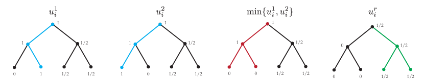
Figure 6: From left to right: two simple models and corresponding u-values with optimal sequences in blue; the naive version of the robust values returns sub-optimal paths in red; our robust U-value properly recovers the robust policy in green.

References

- Abbasi-Yadkori & Szepesvári [2011] Abbasi-Yadkori, Y. and Szepesvári, C. Regret bounds for the adaptive control of linear quadratic systems. In Kakade, S. M. and von Luxburg, U. (eds.), Proceedings of the 24th Annual Conference on Learning Theory, volume 19 of Proceedings of Machine Learning Research, pp. 1–26, Budapest, Hungary, 09–11 Jun 2011. PMLR.
- Abbasi-Yadkori et al. [2011] Abbasi-Yadkori, Y., Pál, D., and Szepesvári, C. Improved algorithms for linear stochastic bandits. In Shawe-Taylor, J., Zemel, R. S., Bartlett, P. L., Pereira, F., and Weinberger, K. Q. (eds.), Advances in Neural Information Processing Systems 24, pp. 2312–2320. Curran Associates, Inc., 2011.
- Abeille & Lazaric [2018] Abeille, M. and Lazaric, A. Improved regret bounds for thompson sampling in linear quadratic control problems. In Dy, J. and Krause, A. (eds.), Proceedings of the 35th International Conference on Machine Learning, volume 80 of Proceedings of Machine Learning Research, pp. 1–9, Stockholmsmässan, Stockholm Sweden, 10–15 Jul 2018. PMLR.
- Adetola et al. [2009] Adetola, V., DeHaan, D., and Guay, M. Adaptive model predictive control for constrained nonlinear systems. Systems and Control Letters, 2009. ISSN 01676911. doi: 10.1016/j.sysconle.2008.12.002.
- Amos et al. [2018] Amos, B., Rodriguez, I. D. J., Sacks, J., Boots, B., and Zico Kolter, J. Differentiable MPC for end-to-end planning and control. In Advances in Neural Information Processing Systems, 2018.
- Aswani et al. [2013] Aswani, A., Gonzalez, H., Sastry, S. S., and Tomlin, C. Provably safe and robust learning-based model predictive control. Automatica, 2013. ISSN 00051098. doi: 10.1016/j.automatica.2013.02.003.
- Basar & Bernhard [1996] Basar, T. and Bernhard, P. H infinity - Optimal Control and Related Minimax Design Problems: A Dynamic Game Approach, volume 41. 1996.
- Ben-Tal et al. [2009] Ben-Tal, A., El Ghaoui, L., and Nemirovski, A. Robust optimization, volume 28. Princeton University Press, 2009.
- Bertsimas et al. [2011] Bertsimas, D., Brown, D. B., and Caramanis, C. Theory and applications of robust optimization. SIAM review, 53(3):464–501, 2011.
- Busoniu et al. [2018] Busoniu, L., Pall, E., and Munos, R. Continuous-action planning for discounted infinite-horizon nonlinear optimal control with lipschitz values. Automatica, 92:100–108, 06 2018.
- Dean et al. [2017] Dean, S., Mania, H., Matni, N., Recht, B., and Tu, S. On the sample complexity of the linear quadratic regulator. ArXiv, abs/1710.01688, 2017.
- Dean et al. [2018] Dean, S., Mania, H., Matni, N., Recht, B., and Tu, S. Regret bounds for robust adaptive control of the linear quadratic regulator. In Bengio, S., Wallach, H., Larochelle, H., Grauman, K., Cesa-Bianchi, N., and Garnett, R. (eds.), Advances in Neural Information Processing Systems 31, pp. 4188–4197. Curran Associates, Inc., 2018.
- Delos & Teissandier [2015] Delos, V. and Teissandier, D. Minkowski Sum of Polytopes Defined by Their Vertices. Journal of Applied Mathematics and Physics (JAMP), 3(1):62–67, January 2015.
- Efimov et al. [2012] Efimov, D., Fridman, L., Raïssi, T., Zolghadri, A., and Seydou, R. Interval estimation for LPV systems applying high order sliding mode techniques. Automatica, 48:2365–2371, 2012.
- Efimov et al. [2013] Efimov, D., Raïssi, T., Chebotarev, S., and Zolghadri, A. Interval state observer for nonlinear time varying systems. Automatica, 49(1):200–205, 2013.
- Faradonbeh et al. [2017] Faradonbeh, M. K. S., Tewari, A., and Michailidis, G. Finite time analysis of optimal adaptive policies for linear-quadratic systems. CoRR, abs/1711.07230, 2017.
- Fukushima et al. [2007] Fukushima, H., Kim, T. H., and Sugie, T. Adaptive model predictive control for a class of constrained linear systems based on the comparison model. Automatica, 2007. ISSN 00051098. doi: 10.1016/j.automatica.2006.08.026.
- Gorissen et al. [2015] Gorissen, B. L., İhsan Yanıkoğlu, and den Hertog, D. A practical guide to robust optimization. Omega, 53:124 – 137, 2015.
- Hren & Munos [2008] Hren, J.-F. and Munos, R. Optimistic planning of deterministic systems. In European Workshop on Reinforcement Learning, pp. 151–164, France, 2008.
- Ibrahimi et al. [2013] Ibrahimi, M., Javanmard, A., and Roy, B. Efficient reinforcement learning for high dimensional linear quadratic systems. Advances in Neural Information Processing Systems, 4, 03 2013.
- Iyengar [2005] Iyengar, G. N. Robust Dynamic Programming. Mathematics of Operations Research, 30:257–280, 2005.
- Köhler et al. [2019] Köhler, J., Andina, E., Soloperto, R., Müller, M. A., and Allgöwer, F. Linear robust adaptive model predictive control: Computational complexity and conservatism. In 2019 IEEE 58th Conference on Decision and Control (CDC), pp. 1383–1388, 2019.
- Kumar & Jerome [2013] Kumar, E. V. and Jerome, J. Robust lqr controller design for stabilizing and trajectory tracking of inverted pendulum. Procedia Engineering, 64:169 – 178, 2013. International Conference on Design and Manufacturing.
- Lenz et al. [2015] Lenz, I., Knepper, R. A., and Saxena, A. Deepmpc: Learning deep latent features for model predictive control. In Robotics: Science and Systems, 2015.
- Leurent [2018] Leurent, E. An environment for autonomous driving decision-making. https://github.com/eleurent/highway-env, 2018.
- Leurent & Mercat [2019] Leurent, E. and Mercat, J. Social attention for autonomous decision-making in dense traffic. In Machine Learning for Autonomous Driving Workshop at NeurIPS 2019, 2019.
- Leurent et al. [2019] Leurent, E., Efimov, D., Raïssi, T., and Perruquetti, W. Interval prediction for continuous-time systems with parametric uncertainties. In Proc. IEEE Conference on Decision and Control (CDC), Nice, 2019.
- Leurent et al. [2020] Leurent, E., Efimov, D., and Maillard, O.-A. Robust-Adaptive Interval Predictive Control for Linear Uncertain Systems. In 2020 IEEE 59th Conference on Decision and Control (CDC), Jeju Island, Republic of Korea, 8–11 Dec 2020.
- Levine et al. [2015] Levine, S., Finn, C., Darrell, T., and Abbeel, P. End-to-end training of deep visuomotor policies. CoRR, abs/1504.00702, 2015.
- Lorenzen et al. [2017] Lorenzen, M., Allgöwer, F., and Cannon, M. Adaptive model predictive control with robust constraint satisfaction. IFAC-PapersOnLine, 50(1):3313–3318, Jul 2017. ISSN 2405-8963.
- Lu & Cannon [2019] Lu, X. and Cannon, M. Robust adaptive tube model predictive control. In Proceedings of the American Control Conference, 2019. ISBN 9781538679265.
- Lu & Spurgeon [1997] Lu, X.-Y. and Spurgeon, S. K. Robust sliding mode control of uncertain nonlinear systems. Systems & Control Letters, 32(2):75–90, Nov 1997. ISSN 0167-6911.
- Mnih et al. [2015] Mnih, V., Kavukcuoglu, K., Silver, D., Rusu, A. A., Veness, J., Bellemare, M. G., Graves, A., Riedmiller, M., Fidjeland, A. K., Ostrovski, G., Petersen, S., Beattie, C., Sadik, A., Antonoglou, I., King, H., Kumaran, D., Wierstra, D., Legg, S., and Hassabis, D. Human-level control through deep reinforcement learning. Nature, 518(7540):529–533, February 2015.
- Nilim & El Ghaoui [2005] Nilim, A. and El Ghaoui, L. Robust Control of Markov Decision Processes with Uncertain Transition Matrices. Operations Research, 53:780–798, 2005.
- Ouyang et al. [2017] Ouyang, Y., Gagrani, M., and Jain, R. Learning-based control of unknown linear systems with thompson sampling. CoRR, abs/1709.04047, 2017.
- Peña et al. [2008] Peña, V. H., Lai, T. L., and Shao, Q.-M. Self-normalized processes: Limit theory and Statistical Applications. Springer Science & Business Media, 2008.
- Rosolia & Borrelli [2019] Rosolia, U. and Borrelli, F. Sample-Based Learning Model Predictive Control for Linear Uncertain Systems. In Proceedings of the IEEE Conference on Decision and Control, 2019. ISBN 9781728113982. doi: 10.1109/CDC40024.2019.9030270.
- Sastry et al. [1990] Sastry, S., Bodson, M., and Bartram, J. F. Adaptive Control: Stability, Convergence, and Robustness. The Journal of the Acoustical Society of America, 1990. ISSN 0001-4966. doi: 10.1121/1.399905.
- Schneider [1997] Schneider, J. Exploiting model uncertainty estimates for safe dynamic control learning. Advances in neural information processing systems, pp. 1047—-1053, 1997.
- Silver et al. [2018] Silver, D., Hubert, T., Schrittwieser, J., Antonoglou, I., Lai, M., Guez, A., Lanctot, M., Sifre, L., Kumaran, D., Graepel, T., Lillicrap, T., Simonyan, K., and Hassabis, D. A general reinforcement learning algorithm that masters chess, shogi, and go through self-play. Science, 362(6419):1140–1144, 2018.
- Tanaskovic et al. [2014] Tanaskovic, M., Fagiano, L., Smith, R., and Morari, M. Adaptive receding horizon control for constrained MIMO systems. Automatica, 2014. ISSN 00051098. doi: 10.1016/j.automatica.2014.10.036.
- Turchetta et al. [2016] Turchetta, M., Berkenkamp, F., and Krause, A. Safe exploration in finite Markov decision processes with Gaussian processes. In Advances in Neural Information Processing Systems, 2016.
- Weinstein & Littman [2012] Weinstein, A. and Littman, M. Bandit-based planning and learning in continuous-action markov decision processes. Proceedings of the 22nd International Conference on Automated Planning and Scheduling, pp. 306–314, 01 2012.
- Wiesemann et al. [2013] Wiesemann, W., Kuhn, D., and Rustem, B. Robust Markov Decision Processes. Mathematics of Operations Research, pp. 1–52, 2013.