Testing Goodness of Fit of Conditional Density Models with Kernels

Abstract

We propose two nonparametric statistical tests of goodness of fit for conditional distributions: given a conditional probability density function $p(\mathbf{y}|\mathbf{x})$ and a joint sample, decide whether the sample is drawn from $p(\mathbf{y}|\mathbf{x})r_{x}(\mathbf{x})$ for some density $r_{x}$. Our tests, formulated with a Stein operator, can be applied to any differentiable conditional density model, and require no knowledge of the normalizing constant. We show that 1) our tests are consistent against any fixed alternative conditional model; 2) the statistics can be estimated easily, requiring no density estimation as an intermediate step; and 3) our second test offers an interpretable test result providing insight on where the conditional model does not fit well in the domain of the covariate. We demonstrate the interpretability of our test on a task of modeling the distribution of New York City’s taxi drop-off location given a pick-up point. To our knowledge, our work is the first to propose such conditional goodness-of-fit tests that simultaneously have all these desirable properties.

1 INTRODUCTION

Conditional distributions provide a versatile tool for capturing the relationship between a target variable and a conditioning variable (or covariate). The last few decades has seen a broad range of modeling applications across multiple disciplines including econometrics in particular (Moreira, 2003; Zheng, 2000), machine learning (Dutordoir et al., 2018; Uria et al., 2016), among others. In many cases, estimating a conditional density function from the observed data is a one of the first crucial steps in the data analysis pipeline. While the task of conditional density estimation has received a considerable attention in the literature, fewer works have investigated the equally important task of evaluating the goodness of fit of a given conditional density model.

Several approaches that address the task of conditional model evaluation take the form of a hypothesis test. Given a conditional density model, and a joint sample containing realizations of both target variables and covariates, test the null hypothesis stating that the model is correctly specified, against the alternative stating that it is not. The model does not specify the marginal distribution of the covariates. We refer to this task as conditional goodness-of-fit testing. One of the early nonparametric tests is Andrews (1997), which extended the classic Kolmogorov test to the conditional case. Zheng (2000) considered the first-order linear expansion of the Kullback-Leibler divergence as the test statistic, and showed that the resulting test is consistent against any fixed alternative under technical assumptions. The conditional Kolmogorov test however requires estimation of the cumulative distribution function (CDF), and may only be applied to data of low dimension. Zheng’s test involves density estimation as part the test statistic, and test consistency is only guaranteed with a decaying smoothing bandwidth whose rate can be challenging to control. While there are other tests which are more computationally tractable, these tests are only designed for conditional models from a specific family: Moreira (2003) for structural equation models, Stute and Zhu (2002) for generalized linear models, to name a few.

Another line of work which is prominent in econometrics is based on the conditional moment restrictions (CMR). In CMR based tests, the conditional model is specified by a conditional moment function which has an important property that its conditional expectation under the true data distribution is zero if and only if the model is correct. This formulation is general, and in fact nests testing a conditional mean regression model as a special case. To guarantee consistency, Bierens and Ploberger (1997); Bierens (1990) use a class of weight functions indexed by a continuous nuisance parameter so that an infinite number of moment conditions can be considered, resulting in a powerful test which detects any departure from the null model. For testing the conditional mean of a regression model, the conditional moment function can be set to the squared loss between the model output and the target variable. However, for testing the goodness of fit of a conditional density model, specifying the conditional moment function is challenging, especially for a complex model whose normalizing constant is intractable.

A related thread of development of omnibus tests for model goodness of fit has arisen in the machine learning community recently through the use of kernel methods and Stein operators. The combination of Stein’s identity and kernel methods was investigated in Oates et al. (2017) for the purpose of reducing the variance of Monte Carlo integration. Chwialkowski et al. (2016); Liu et al. (2016) independently proposed a consistent, nonparametric test of goodness of fit of a marginal density model known as the Kernel Stein Discrepancy (KSD) test. The KSD test has proved successful in many applications and has spawned a number of further studies including Gorham and Mackey (2017) which considered the KSD for checking the convergence of an MCMC procedure, Yang et al. (2018) which extended the KSD test to a discrete domain, and Huggins and Mackey (2018); Jitkrittum et al. (2017a) which developed linear-time variants of the KSD. While proven to be powerful, an issue with the KSD is that it is only applicable to marginal (unconditional) density models. To our knowledge, there has been no attempt of extending the KSD test to handle conditional density models.

In the present work, we are interested in constructing omnibus statistics which can detect any departure from the specified conditional density model in the null hypothesis. We propose two nonparametric, general conditional goodness-of-fit tests which require no density estimation as an intermediate step. Our first test, the Kernel Conditional Stein Discrepancy (KCSD, described in Section 3), generalizes the KSD to conditional goodness-of-fit testing. Briefly, we consider the KSD’s Stein witness function conditioned on the covariate. The KCSD statistic is defined as the norm, in a vector-valued reproducing kernel Hilbert space (RKHS), of a kernel integral operator applied to the conditional witness function. The use of the kernel integral operator ensures that the discrepancy between the conditional model and the data can be detected for any realization of the conditioning variable. We prove that the KCSD test is consistent against any fixed alternative conditional model, for any $C_{0}$-universal positive definite kernels used; importantly, in the case of Gaussian kernels, the consistency holds regardless of the bandwidth parameter (not necessarily decaying in contrast to Zheng (2000)).

Our second proposed test, referred to as the Finite Set Conditional Discrepancy (FSCD, described in Section 4), further extends the KCSD test to also return test locations (a set of points) that indicate realizations of the covariate at which the conditional model does not fit well. The FSCD test thus offers an interpretable indication of where the conditional model fails as evidence for rejecting the null hypothesis. Thanks to the Stein operator, our proposed tests do not require the normalizing constant of the conditional model. In experiments on both homoscedastic and heteroscedastic models, we show that the KCSD test is suited for detecting global differences, whereas the use of test locations in the FSCD makes it more sensitive to local departure from the null model.

2 BACKGROUND

This section gives background materials which will be needed when we propose our new tests: the Kernel Conditional Stein Discrepancy (KCSD, Section 3) and the Finite Set Conditional Discrepancy (FSCD, Section 4). We describe two known (unconditional) goodness-of-fit tests: the Kernel Stein Discrepancy (KSD) test of Chwialkowski et al. (2016); Liu et al. (2016) in Section 2.1, and the Finite Set Stein Discrepancy (FSSD) of Jitkrittum et al. (2017b) in Section 2.2. We will see in Sections 3 and 4 that our proposed KCSD and FSCD are generalizations of KSD and FSSD, respectively, to the conditional goodness-of-fit testing problem.

2.1 KERNEL STEIN DISCREPANCY (KSD)

Consider probability distributions supported on an open subset $\mathcal{X}\subseteq\mathbb{R}^{d}$ for $d\in\mathbb{N}$. The Kernel Stein Discrepancy (KSD) between probability distributions $P$ and $R$ is a divergence measure defined as $S_{P}(R)\coloneqq\sup_{\|\mathbf{f}\|_{\mathcal{F}^{d}}\leq 1}\left|\mathbb{E}_{\mathbf{x}\sim R}T_{P}\mathbf{f}(\mathbf{x})-\mathbb{E}_{\mathbf{x}\sim P}T_{P}\mathbf{f}(\mathbf{x})\right|$, where $\mathbf{f}\in\mathcal{F}^{d}$, $\mathcal{F}^{d}=\times_{j=1}^{d}\mathcal{F}$, and $\mathcal{F}$ is the reproducing kernel Hilbert space (RKHS, Berlinet and Thomas-Agnan (2011)) associated with a positive definite kernel $k:\mathbb{R}^{d}\times\mathbb{R}^{d}\to\mathbb{R}$.

Key to the KSD is $T_{P}$, a Stein operator constructed such that the expectation under the distribution $P$ vanishes, i.e., $\mathbb{E}_{\mathbf{x}\sim P}T_{P}\mathbf{f}(\mathbf{x})=0$, for any function $\mathbf{f}\in\mathcal{F}^{d}$. For a distribution $P$ admitting a differentiable, strictly positive density $p:\mathcal{X}\to(0,\infty)$, the Langevin Stein operator of differentiable functions defined by $T_{p}\mathbf{f}(\mathbf{x})=\mathbf{s}_{p}(\mathbf{x)}{}^{\top}\mathbf{f}(\mathbf{x})+\nabla_{\mathbf{x}}\mathbf{f}(\mathbf{x})\in\mathbb{R}^{d}$ satisfies the aforementioned condition, where $\mathbf{s}_{p}(\mathbf{x}):=\nabla_{\mathbf{x}}\log p(\mathbf{x})$ is the score function (under suitable boundary conditions (Oates et al., 2017, Assumption A2’)). Thus, the KSD can be equivalently written as $\sup_{\|\mathbf{f}\|_{\mathcal{F}^{d}}\leq 1}\left|\mathbb{E}_{\mathbf{x}\sim R}T_{p}\mathbf{f}(\mathbf{x})\right|$ It can be shown that if the kernel $k$ is $C_{0}$-universal (Sriperumbudur et al., 2011), and $R$ has a density $r$ such that $\mathbb{E}_{\mathbf{x}\sim r}\lVert\nabla_{\mathbf{x}}\log p(\mathbf{x})-\nabla_{\mathbf{x}}\log r(\mathbf{x})\rVert_{2}^{2}<\infty$, then $S_{p}(r)=0$ if and only if $p=r$ (Chwialkowski et al., 2015, Theorem 2.2).

The KSD can be rewritten in a form that can be estimated easily. Assume that the kernel $k$ is differentiable. Then, for any function $\mathbf{f}\in\mathcal{F}^{d}$, we have $T_{p}\mathbf{f}(\mathbf{x})=\langle\mathbf{f},\xi_{p}(\mathbf{x},\cdot)\rangle_{\mathcal{F}^{d}}$ where $\xi_{p}(\mathbf{x},\cdot):=\mathbf{s}_{p}(\mathbf{x})k(\mathbf{x},\cdot)+\nabla_{x}k(\mathbf{x},\cdot)$, due to the reproducing property of $k$, where $\langle\mathbf{f},\mathbf{g}\rangle_{\mathcal{F}^{d}}=\sum_{j=1}^{d}\langle f_{j},g_{j}\rangle_{\mathcal{F}}$ is the inner product on $\mathcal{F}^{d}$. Assuming Bochner integrability of $\xi_{p}(\mathbf{x},\cdot)$ as in Chwialkowski et al. (2016); Liu et al. (2016), it follows that

$$S_{p}(r) =\sup_{\mathbf{f}\in\mathcal{F}^{d}}\left|\langle\mathbf{f},\mathbb{E}_{\mathbf{x}\sim r}\xi_{p}(\mathbf{x},\cdot)\rangle_{\mathcal{F}^{d}}\right|=\lVert\mathbf{g}_{p,r}\rVert_{\mathcal{F}^{d},}$$

where $\mathbf{g}_{p,r}(\cdot)=\mathbb{E}_{\mathbf{x}\sim r}\xi_{p}(\mathbf{x},\cdot)\in\mathcal{F}^{d}$ is the function that achieves the supremum, and is known as the Stein witness function (Jitkrittum et al., 2017a). The squared KSD admits the expression $S_{p}^{2}(r)=\lVert\mathbf{g}_{p,r}\rVert_{\mathcal{F}^{d},}^{2}=\mathbb{E}_{\mathbf{x},\mathbf{x}^{\prime}\sim r}h_{p}(\mathbf{x},\mathbf{x}^{\prime})$ where

$$h_{p}(\mathbf{x,\mathbf{x}^{\prime}}): =k(\mathbf{x},\mathbf{x}^{\prime})\mathbf{s}_{p}^{\top}(\mathbf{x})\mathbf{s}_{p}(\mathbf{x}^{\prime})+\sum_{i=1}^{d}\frac{\partial^{2}k(\mathbf{x},\mathbf{x}^{\prime})}{\partial x_{i}\partial x_{i}^{\prime}}$$

$$\phantom{=}+\mathbf{s}_{p}^{\top}(\mathbf{x})\nabla_{\mathbf{x}^{\prime}}k(\mathbf{x},\mathbf{x}^{\prime})+\mathbf{s}_{p}^{\top}(\mathbf{x}^{\prime})\nabla_{\mathbf{x}}k(\mathbf{x},\mathbf{x}^{\prime}).$$

Given a sample $\{\mathbf{x}_{i}\}_{i=1}^{n}\sim r$, the squared KSD has an unbiased estimator $\hat{S}_{p}^{2}(r)\coloneqq\frac{1}{n(n-1)}\sum_{i\neq j}h_{p}(\mathbf{x}_{i},\mathbf{x}_{j})$, which is a U-statistic (Serfling, 2009). Since the KSD only depends on $p$ through $\nabla_{\mathbf{x}}\log p(\mathbf{x})$, the normalizing constant of $p$ is not required. The squared KSD has been successfully used in Chwialkowski et al. (2016); Liu et al. (2016) as the test statistic for goodness-of-fit testing: given a marginal density model $p$ (known up to the normalizing constant), and a sample $\{\mathbf{x}_{i}\}_{i=1}^{n}\sim r$, test whether $p$ is the correct model.

2.2 FINITE SET STEIN DISCREPANCY (FSSD)

The Finite Set Stein Discrepancy (FSSD, Jitkrittum et al. (2017a)) is one of several extensions of the original KSD aiming to construct a goodness-of-fit test of an unconditional density model that runs in linear time (i.e., $\mathcal{O}(n)$ runtime complexity), and that offers an interpretable test result. Key to the FSSD is the observation that the KSD $S_{p}(r)=0$ if and only if $p=r$, assuming conditions described in Section 2.1. As a result, $\mathbf{g}_{p,r}$ is a zero function if and only if $p=r$, implying that the departure of $\mathbf{g}_{p,r}$ from the zero function can be used to determine whether $p$ and $r$ are the same. In contrast to the KSD which relies on the RKHS norm $\|\cdot\|_{\mathcal{F}^{d}}$, the FSSD statistic evaluates the Stein witness function to check this departure. Specifically, given a finite set $V:=\{\mathbf{v}_{1},\ldots,\mathbf{v}_{J}\}\subset\mathcal{X}$ (known as the set of test locations), the squared FSSD is defined as $\mathrm{FSSD}_{p}^{2}(r):=\frac{1}{dJ}\sum_{j=1}^{J}\|\mathbf{g}_{p,r}(\mathbf{v}_{j})\|_{2}^{2}$. It is shown in Jitkrittum et al. (2017b) that if $V$ is drawn from a distribution with a density supported on $\mathcal{X}$, then $\mathrm{FSSD}_{p}^{2}(r)=0$ if and only if $p=r$. The squared FSSD can be estimated in linear time, and $V$ can be optimized by maximizing the test power of the FSSD statistic. The optimized $V$ reveals where $p$ and $r$ differ.

3 THE KERNEL CONDITIONAL STEIN DISCREPANCY (KCSD)

In this section, we propose our first test statistic called the Kernel Conditional Stein Discrepancy (KCSD) for distinguishing two conditional probability density functions. All omitted proofs can be found in Section A (appendix).

Problem Setting Let $X$ and $Y$ be two random vectors taking values in $\mathcal{X}\times\mathcal{Y}\subset\mathbb{R}^{d_{x}}\times\mathbb{R}^{d_{y}}$. Let $p=p(\mathbf{y}|\mathbf{x})$ be a conditional density function representing a candidate model for modeling the conditional distribution of $\mathbf{y}$ given $\mathbf{x}$. Given a joint sample $Z_{n}=\{(\mathbf{x}_{i},\mathbf{y}_{i})\}_{i=1}^{n}\stackrel{{\scriptstyle i.i.d.}}{{\sim}}r_{xy}$ where $r_{xy}(\mathbf{x},\mathbf{y})=r(\mathbf{y}|\mathbf{x})r_{x}(\mathbf{x})$ is a joint density defined on $\mathcal{X}\times\mathcal{Y}$, conditional goodness-of-fit testing tests

$$H_{0}\colon p \stackrel{{\scriptstyle r_{x}}}{{=}}r\text{ $\quad$vs$\quad$}H_{1}\colon p\stackrel{{\scriptstyle r_{x}}}{{\neq}}r,$$ (1)

where we write $p\stackrel{{\scriptstyle r_{x}}}{{=}}r$ if for $r_{x}$-almost all $\mathbf{x}$ and for all $\mathbf{y}\in\mathcal{Y}$, $p(\mathbf{y}|\mathbf{x})=r(\mathbf{y}|\mathbf{x})$. The alternative hypothesis $H_{1}$ is the negation of $H_{0}$ and is equivalent to the statement “there exists a set $U\subseteq\mathcal{X}$ with $r_{x}(U)>0$ such that $p(\cdot|\mathbf{x})\neq r(\cdot|\mathbf{x})$ for all $\mathbf{x}\in U$.” Note that $r_{xy}$ is only observed through the joint sample $Z_{n}$; and $p$ only specifies the conditional model. That is, $p$ does not specify a marginal model for $\mathbf{x}$. This subtlety is what distinguishes the conditional goodness-of-fit testing from testing the difference between two joint distributions.

Rationale For machine learning applications, the proposed null hypothesis in (1) allows testing the goodness of fit of a wide range of conditional density models, including regression models with homoscedastic or heteroscedastic noise. The underlying prediction function can be a neural network or other arbitrarily nonlinear functions as long as $\nabla_{\mathbf{y}}\log p(\mathbf{y}|\mathbf{x})$ is differentiable, and satisfies conditions in Theorem 1. In this work we consider $Y$ to be a continuous random vector. However, our proposed tests can be extended to handle a discrete $Y$ to allow testing, for instance, Bayesian classifier models $p(y|\mathbf{x})$ where $y$ represents the classification label. While the formulated hypothesis in the current form allows testing only a fixed conditional model (i.e., all model parameters if any must have been learned before the test) and may appear restrictive in some cases, our goal is not to advocate this particular null hypothesis. Rather, we see this formulation as a first step for more realistic null hypotheses that are yet to come; for instance, testing whether $p(\mathbf{y}|\mathbf{x},\theta)=r(\mathbf{y}|\mathbf{x})$ for some parameter vector $\theta\in\Theta$, or testing the relative fit (with respect to the true distribution $r$) of two competing candidate conditional models $p$ and $q$. Future tests that consider these hypotheses can build on the results in this paper. We leave these questions for future work.

Vector-valued reproducing kernels We will require vector-valued reproducing kernels for the construction of our new tests. We briefly give a brief introduction to this concept here. For further details, please see Section 2.2 of Carmeli et al. (2008) and Carmeli et al. (2006); Sriperumbudur et al. (2011); Szabó and Sriperumbudur (2018). Let $\mathcal{L}(\mathcal{H};\mathcal{H}^{\prime})$ be the Banach space of bounded operators from a Hilbert space $\mathcal{H}$ to $\mathcal{H}^{\prime}$ endowed with the uniform norm. We write $\mathcal{L}(\mathcal{H})$ for $\mathcal{L}(\mathcal{H};\mathcal{H})$. A kernel $K\colon\mathcal{X}\times\mathcal{X}\to\mathcal{L}(\mathcal{Z})$ is said to be a $\mathcal{Z}$-reproducing kernel if $\sum_{i=1}^{N}\sum_{j=1}^{N}\left\langle K(\mathbf{x}_{i},\mathbf{x}_{j})\mathbf{z}_{i},\mathbf{z}_{j}\right\rangle_{\mathcal{Z}}\geq 0$ for any $N\geq 1,\{\mathbf{x}_{i}\}_{i=1}^{N}\subset\mathcal{X},\{\mathbf{z}_{i}\}_{i=1}^{N}\subset\mathcal{Z},$ and $\left\langle\diamond,\diamond\right\rangle_{\mathcal{Z}}$ denotes the inner product on $\mathcal{Z}$. Given $\mathbf{x}\in\mathcal{X}$, we write $K_{\mathbf{x}}\colon\mathcal{Z}\to\mathcal{L}(\mathcal{X};\mathcal{Z})$ to denote the linear operator such that $K_{\mathbf{x}}\mathbf{z}\in\mathcal{L}(\mathcal{X};\mathcal{Z})$ and $(K_{\mathbf{x}}\mathbf{z})(\mathbf{t})=K(\mathbf{x},\mathbf{t})\mathbf{z}\in\mathcal{Z}$, for all $\mathbf{x},\mathbf{t}\in\mathcal{X}$ and all $\mathbf{z}\in\mathcal{Z}$. As in the case of a real-valued reproducing kernel, given a $\mathcal{Z}$-reproducing kernel $K$, there exists a unique reproducing kernel Hilbert space (RKHS) $\mathcal{F}_{K}$ such that $K_{\mathbf{x}}\in\mathcal{L}(\mathcal{Z};\mathcal{F}_{K})$ and $f(\mathbf{x})=K_{\mathbf{x}}^{*}f$ (the reproducing property) for all $\mathbf{x}\in\mathcal{X},f\in\mathcal{F}_{K}$ and $K_{\mathbf{x}}^{*}\colon\mathcal{F}_{K}\to\mathcal{Z}$ denotes the adjoint operator of $K_{\mathbf{x}}$.

Let $\mathcal{C}(\mathcal{X};\mathcal{Z})$ be the vector space of continuous functions mapping from $\mathcal{X}$ to $\mathcal{Z}$. In this work, we will assume that $\mathcal{X}$ and $\mathcal{Z}$ are Banach spaces. Let $\mathcal{C}_{0}(\mathcal{X};\mathcal{Z})\subset\mathcal{C}(\mathcal{X};\mathcal{Z})$ denote the subspace of continuous functions that vanish at infinity i.e., $\|f(\mathbf{x})\|_{\mathcal{Z}}\to 0$ as $\|\mathbf{x}\|\to\infty$. A $\mathcal{Z}$-reproducing kernel $K\colon\mathcal{X}\times\mathcal{X}\to\mathcal{L}(\mathcal{Z})$ is said to be $C_{0}$ if $\mathcal{F}_{K}$ is a subspace of $\mathcal{C}_{0}(\mathcal{X};\mathcal{Z})$ (Carmeli et al., 2008, Section 2.3, Definition 1). A $C_{0}$-kernel $K$ is said to be universal if $\mathcal{F}_{K}$ is dense in $L^{2}(\mathcal{X},\mu;\mathcal{Z})$ for any probability measure $\mu$ (Carmeli et al., 2008, Section 4.1).

Let $l\colon\mathcal{Y}\times\mathcal{Y}\to\mathbb{R}$ be a positive definite kernel associated with the RKHS $\mathcal{F}_{l}$. Write $\mathcal{F}_{l}^{d_{y}}:=\times_{i=1}^{d_{y}}\mathcal{F}_{l}$ and define $\left\langle\mathbf{a},\mathbf{b}\right\rangle_{\mathcal{F}_{l}^{d_{y}}}:=\sum_{i=1}^{d_{y}}\left\langle a_{i},b_{i}\right\rangle_{\mathcal{F}_{l}}$ to be the inner product on $\mathcal{F}_{l}^{d_{y}}$ for $\mathbf{a}:=(a_{1},\ldots,a_{d_{y}}),\mathbf{b}:=(b_{1},\ldots,b_{d_{y}})\in\mathcal{F}_{l}^{d_{y}}$. Let $K\colon\mathcal{X}\times\mathcal{X}\to\mathcal{F}_{l}^{d_{y}}$ be a $\mathcal{F}_{l}^{d_{y}}$-reproducing kernel i.e., $\mathcal{Z}=\mathcal{F}_{l}^{d_{y}}$. Let $k\colon\mathcal{X}\times\mathcal{X}\to\mathbb{R}$ be a real-valued kernel associated with the RKHS $\mathcal{F}_{k}$. For brevity, we write $\mathbb{E}_{\mathbf{xy}}$ for $\mathbb{E}_{(\mathbf{x},\mathbf{y})\sim r_{xy}}$. In what follows, we will interchangeably write $p_{|\mathbf{x}}$ and $p(\cdot|\mathbf{x})$.

Proposed statistic Consider the following population statistic defining a discrepancy between $p$ and $r$:

$$D_{p}(r): =\big{\|}\mathbb{E}_{(\mathbf{x},\mathbf{y})\sim r_{xy}}K_{\mathbf{x}}\xi_{p_{|\mathbf{x}}}(\mathbf{y},\diamond)\big{\|}_{\mathcal{F}_{K}}^{2},$$ (2)

where $\xi_{p_{|\mathbf{x}}}(\mathbf{y},\cdot):=l(\mathbf{y},\cdot)\nabla_{\mathbf{y}}\log p(\mathbf{y}|\mathbf{x})+\nabla_{\mathbf{y}}l(\mathbf{y},\cdot)\in\mathcal{F}_{l}^{d_{y}}$. We refer to $D_{p}(r)$ as the Kernel Conditional Stein Discrepancy (KCSD). Our first result in Theorem 1 shows that the KCSD is zero if and only if $p\stackrel{{\scriptstyle r_{x}}}{{=}}r$.

Theorem 1 ($D_{p}(r)$ distinguishes conditional density functions).

Let $K\colon\mathcal{X}\times\mathcal{X}\to\mathcal{L}(\mathcal{F}_{l}^{d_{y}})$ and $l\colon\mathcal{Y}\times\mathcal{Y}\to\mathbb{R}$ be positive definite kernels. Define $\mathbf{g}_{p,r}(\mathbf{w}|\mathbf{x}):=\mathbb{E}_{\mathbf{y}\sim r_{|\mathbf{x}}}\xi_{p_{|\mathbf{x}}}(\mathbf{y},\mathbf{w})\in\mathbb{R}^{d_{y}}$ where $\mathbf{g}_{p,r}(\cdot|\mathbf{x})\in\mathcal{F}_{l}^{d_{y}}$ for each $\mathbf{x}$. Assume that

1. $K$ and $l$ are $C_{0}$-universal;

2. $r_{x}\mbox{-}\mathrm{ess}\sup_{\mathbf{x}}\mathbb{E}_{\mathbf{y}\sim r(\mathbf{y}|\mathbf{x})}\big{\|}\nabla_{\mathbf{y}}\log\frac{p(\mathbf{y}|\mathbf{x})}{r(\mathbf{y}|\mathbf{x})}\big{\|}_{2}^{2}<\infty$;

3. $\int_{\mathcal{X}}\|\mathbf{g}_{p,r}(\diamond|\mathbf{x})\|_{\mathcal{F}_{l}^{d_{y}}}^{2}r_{x}(\mathbf{x})\thinspace\mathrm{d}\mathbf{x}<\infty$.

4. $\mathbb{E}_{\mathbf{xy}}\|K_{\mathbf{x}}\xi_{p_{|\mathbf{x}}}(\mathbf{y},\diamond)\|_{\mathcal{F}_{K}}<\infty$;

Then $D_{p}(r)=0$ if and only if $p\stackrel{{\scriptstyle r_{x}}}{{=}}r$ i.e., for $r_{x}$-almost all $\mathbf{x}\in\mathcal{X}$, $p(\cdot|\mathbf{x})=r(\cdot|\mathbf{x})$.

Proof (sketch).

The idea is to rewrite (2) into a form that involves the Stein witness function (as described in Section 2) $\mathbf{g}_{p,r}(\diamond|\mathbf{x})$ between $p(\cdot|\mathbf{x})$ and $r(\cdot|\mathbf{x})$. It then amounts to showing that $\mathbf{g}_{p,r}(\diamond|\mathbf{x})$ is a zero function for $r_{x}$-almost all $\mathbf{x}$. This is done by applying the integral operator $\mathbf{f}_{\mathbf{x}}\mapsto\int K_{\mathbf{x}}\mathbf{f}_{\mathbf{x}}r_{x}(\mathbf{x})\thinspace\mathrm{d}\mathbf{x}$ on $\mathbf{g}_{p,r}(\diamond|\mathbf{x})$ to incorporate ($r_{x}$-almost) all $\mathbf{x}$. The result is $G_{p,r}=\int K_{\mathbf{x}}\mathbf{g}_{p,r}(\diamond|\mathbf{x})r_{x}(\mathbf{x})\thinspace\mathrm{d}\mathbf{x}$. Since $K$ is $C_{0}$-universal, this operator is injective, implying $G_{p,r}$ is zero if and only if $\mathbf{g}_{p,r}(\diamond|\mathbf{x})$ is a zero function for $r_{x}$-almost all $\mathbf{x}$. But, $G_{p,r}=\mathbb{E}_{(\mathbf{x},\mathbf{y})\sim r_{xy}}K_{\mathbf{x}}\xi_{p_{|\mathbf{x}}}(\mathbf{y},\diamond)$. Thus, taking the norm gives (2). See Section A.1 for the complete proof. ∎

In the proof sketch, we can see the application of the integral operator $\mathbf{f}_{\mathbf{x}}\mapsto\int K_{\mathbf{x}}\mathbf{f}_{\mathbf{x}}r_{x}(\mathbf{x})\thinspace\mathrm{d}\mathbf{x}$ as taking into account the conditional Stein witness function $\mathbf{g}_{p,r}(\diamond|\mathbf{x})$ of ($r_{x}$-almost) all $\mathbf{x}$ at the same time. Theorem 1 states that the population statistic in (2) distinguishes two conditional density functions under regularity conditions given above. In particular, it is required that the two kernels $K$ and $l$ are $C_{0}$-universal. Examples of a real-valued $C_{0}$-universal kernels are the Gaussian kernel $l(\mathbf{y},\mathbf{y}^{\prime}):=\exp\left(-\frac{\|\mathbf{y}-\mathbf{y}^{\prime}\|_{2}^{2}}{2\sigma_{y}^{2}}\right)\in\mathbb{R}$, Laplace kernel, and the inverse multiquadrics kernel (Sriperumbudur et al., 2011, p. 2397). An example of a $\mathcal{F}_{l}^{d_{y}}$-reproducing, $C_{0}$-universal kernel $K$ is $K(\mathbf{x},\mathbf{x}^{\prime})=k(\mathbf{x},\mathbf{x}^{\prime})I$ where $k$ is a real-valued $C_{0}$-universal kernel, and $I\in\mathcal{L}(\mathcal{F}_{l}^{d_{y}})$ is the identity operator (Carmeli et al., 2008, Example 14). For simplicity, in this work, we will assume a kernel $K$ that takes this form.

3.1 HYPOTHESIS TESTING WITH KCSD

To construct a statistical test for conditional goodness of fit, we start by rewriting $D_{p}(r)$ in (2) in a form that can be estimated easily as shown in Proposition 2.

Proposition 2.

Assume that $K(\mathbf{x},\mathbf{x}^{\prime}):=k(\mathbf{x},\mathbf{x}^{\prime})I$ for a positive definite kernel $k\colon\mathcal{X}\times\mathcal{X}\to\mathbb{R}$. Define $\mathbf{s}_{p}(\mathbf{y}|\mathbf{x}):=\nabla_{\mathbf{y}}\log p(\mathbf{y}|\mathbf{x})$. Then,

$$D_{p}(r)=\mathbb{E}_{\mathbf{xy}}\mathbb{E}_{\mathbf{x^{\prime}y^{\prime}}}k(\mathbf{x},\mathbf{x}^{\prime})h_{p}((\mathbf{x},\mathbf{y}),(\mathbf{x}^{\prime},\mathbf{y}^{\prime})),$$ (3)

where $h_{p}((\mathbf{x},\mathbf{y}),(\mathbf{x}^{\prime},\mathbf{y}^{\prime}))$

$$:=l(\mathbf{y},\mathbf{y}^{\prime})\mathbf{s}_{p}^{\top}(\mathbf{y}|\mathbf{x})\mathbf{s}_{p}(\mathbf{y}^{\prime}|\mathbf{x}^{\prime})+\sum_{i=1}^{d_{y}}\frac{\partial^{2}}{\partial y_{i}\partial y_{i}^{\prime}}l(\mathbf{y},\mathbf{y}^{\prime})$$

$$\phantom{:=}+\mathbf{s}_{p}^{\top}(\mathbf{y}|\mathbf{x})\nabla_{\mathbf{y}^{\prime}}l(\mathbf{y},\mathbf{y}^{\prime})+\mathbf{s}_{p}^{\top}(\mathbf{y}^{\prime}|\mathbf{x}^{\prime})\nabla_{\mathbf{y}}l(\mathbf{y},\mathbf{y}^{\prime}),$$ (4)

Define $H_{p}((\mathbf{x},\mathbf{y}),(\mathbf{x}^{\prime},\mathbf{y}^{\prime})):=k(\mathbf{x},\mathbf{x}^{\prime})h_{p}((\mathbf{x},\mathbf{y}),(\mathbf{x}^{\prime},\mathbf{y}^{\prime}))$. Given an i.i.d. sample $\{(\mathbf{x}_{i},\mathbf{y}_{i})\}_{i=1}^{n}\sim r_{xy}$. an unbiased, consistent estimator for (3) is given by

$$\widehat{D_{p}}:= \frac{1}{n(n-1)}\sum_{i\neq j}H_{p}((\mathbf{x}_{i},\mathbf{y}_{i}),(\mathbf{x}_{j},\mathbf{y}_{j})),$$ (5)

which is a second-order U-statistic with $H_{p}$ as the U-statistic kernel (Serfling, 2009, Section 5), and can be computed easily. It is clear from (4) that the KCSD statistic (both population and its estimator) depends on the model $p$ only through $\nabla_{\mathbf{y}}\log p(\mathbf{y}|\mathbf{x})=\nabla_{\mathbf{y}}\log p(\mathbf{y},\mathbf{x})$ which is independent of the normalizer $p(\mathbf{x})$. The fact that the KCSD does not require the normalizer is a big advantage since modern conditional models tend to be complex and their normalizers may not be tractable. A consequence of being a U-statistic is that its asymptotic behaviors can be derived straightforwardly, as given in Proposition 3.

Proposition 3 (Asymptotic distributions of $\widehat{D_{p}}$).

Assume all conditions in Theorem 1 and assume that $\mathbb{E}_{\mathbf{xy}}\mathbb{E}_{\mathbf{x^{\prime}y^{\prime}}}H_{p}^{2}((\mathbf{x},\mathbf{y}),(\mathbf{x}^{\prime},\mathbf{y}^{\prime}))<\infty$. Then,

1. Under $H_{0}$, $n\widehat{D_{p}}\stackrel{{\scriptstyle d}}{{\to}}\sum_{j=1}^{\infty}\lambda_{j}(\chi_{j1}^{2}-1)$, where $\{\chi_{1j}^{2}\}_{j}$ are independent $\chi_{1}^{2}$ random variables, $\lambda_{j}$ are eigenvalues of the operator $A$ defined as $(A\varphi)(\mathbf{z})=\int H_{p}(\mathbf{z},\mathbf{z}^{\prime})\varphi(\mathbf{z}^{\prime})r_{xy}(\mathbf{z}^{\prime})\thinspace\mathrm{d}\mathbf{z}^{\prime}$ for non-zero $\varphi$, $\mathbf{z}:=(\mathbf{x},\mathbf{y})$ and $\mathbf{z}^{\prime}:=(\mathbf{x}^{\prime},\mathbf{y}^{\prime})$;

2. Under $H_{1}$, $\sqrt{n}\left(\widehat{D_{p}}-D_{p}(r)\right)\stackrel{{\scriptstyle d}}{{\to}}\mathcal{N}(0,\sigma_{H_{1}}^{2})$ where $\sigma_{H_{1}}^{2}:=4\mathbb{V}[\mathbb{E}_{\mathbf{xy}}[H_{p}((\mathbf{x},\mathbf{y}),(\mathbf{x}^{\prime},\mathbf{y}^{\prime}))]]$.

A proof of Proposition 3 can be found in Section A.3 (appendix). Proposition 3 suggests that under $H_{0}$, $n\widehat{D_{p}}$ converges to a limit distribution given by an infinite weighted sum of chi-squared random variables. Under $H_{1}$, for any fixed $p$ and $r$, we have $n\widehat{D_{p}}=\mathcal{O}_{p}(\sqrt{n})$, which diverges to $+\infty$, and allows the test to reject $H_{0}$ when $n$ is sufficiently large. The behaviors are common in many recently developed nonparametric tests (Yang et al., 2018; Chwialkowski et al., 2016; Liu et al., 2016; Gretton et al., 2008, 2012a). A consistent test that has an asymptotic false rejection rate no larger than a specified significance level $\alpha\in(0,1)$ can be constructed by setting the rejection threshold (critical value) to be $\gamma_{1-\alpha}=(1-\alpha)$-quantile of the asymptotic null distribution. That is, the test rejects the null hypothesis $H_{0}$ if $n\widehat{D_{p}}>\gamma_{1-\alpha}$. In practice however, the limiting distribution under $H_{0}$ is not available in closed form, and we have to resort to approximating the test threshold either by bootstrapping (Arcones and Gine, 1992; Huskova and Janssen, 1993) or estimating the eigenvalues $\{\lambda_{j}\}_{j}$ which can cost $\mathcal{O}(n^{3})$ runtime (Gretton et al., 2009).

Test threshold In our work, we use the bootstrap procedure of Arcones and Gine (1992); Huskova and Janssen (1993) as also used in the KSD test of Liu et al. (2016); Yang et al. (2018) (with a U-statistic estimator) and Chwialkowski et al. (2015) (with a V-statistic estimator). To generate a bootstrap sample, we draw $w_{1},\ldots,w_{n}\sim\mathrm{Multinomial}\left(n;\frac{1}{n},\ldots,\frac{1}{n}\right)$, define $\tilde{w}_{i}:=\frac{1}{n}(w_{i}-1)$, and compute $\widehat{D_{p}}^{*}=\sum_{i=1}^{n}\sum_{j\neq i}\tilde{w}_{i}\tilde{w}_{j}H_{p}((\mathbf{x}_{i},\mathbf{y}_{i}),(\mathbf{x}_{i},\mathbf{y}_{j})).$ By bootstrapping $m$ times to generate $\widehat{D_{p}}_{1}^{*},\ldots\widehat{D_{p}}_{m}^{*}$, the test threshold can be estimated by computing the empirical $(1-\alpha)$-quantile of these bootstrapped samples. The overall computational cost of this bootstrap procedure is $\mathcal{O}(mn^{2})$, which is the same cost as testing a marginal probability model in the KSD test.

4 THE FINITE SET CONDITIONAL DISCREPANCY (FSCD)

In this section, we extend the KCSD statistic presented in Section 3 to enable it to also pinpoint the location(s) in the domain of $\mathcal{X}$ that best distinguish $p(\cdot|\mathbf{x})$ and $r(\cdot|\mathbf{x})$. The result is a goodness-of-fit test for conditional density functions which gives an interpretable output (in terms of locations in $\mathcal{X})$ to justify a rejection of the null hypothesis.

We start by noting that Theorem 1 and (2) implies that $G_{p,r}\colon\mathcal{X}\to\mathcal{F}_{l}^{d_{y}}$ defined as $G_{p,r}(\mathbf{v}):=\left[\mathbb{E}_{(\mathbf{x},\mathbf{y})\sim r_{xy}}K_{\mathbf{x}}\xi_{p_{|\mathbf{x}}}(\mathbf{y},\diamond)\right](\mathbf{v})\in\mathcal{F}_{l}^{d_{y}}$ is a zero function if and only if $p\stackrel{{\scriptstyle r_{x}}}{{=}}r$, under the conditions described in the theorem statement. Note that the KCSD $D_{p}(r)=\|G_{p,r}\|_{\mathcal{F}_{K}}^{2}$. For a fixed $\mathbf{v}\in\mathcal{X}$, the function $\mathbf{v}\mapsto\frac{1}{d_{y}}\|G(\mathbf{v})\|_{\mathcal{F}_{l}^{d_{y}}}^{2}\geq 0$ can be seen as quantifying the extent to which $p$ and $r$ differ, as measured at $\mathbf{v}\in\mathcal{X}$; that is, the higher $\frac{1}{d_{y}}\|G(\mathbf{v})\|_{\mathcal{F}_{l}^{d_{y}}}^{2}$, the larger the discrepancy between $p(\cdot|\mathbf{v})$ and $r(\cdot|\mathbf{v})$. Inspired by Jitkrittum et al. (2017b), one can thus construct a variant of the KCSD statistic as follows. Given a set of $J$ test locations $V:=\{\mathbf{v}_{i}\}_{i=1}^{J}\subset\mathcal{X}$, we evaluate $G_{p,r}(\mathbf{v})$ at these locations instead of taking the norm $\|\cdot\|_{\mathcal{F}_{K}}$ (Jitkrittum et al., 2016, 2017a, 2017b; Scetbon and Varoquaux, 2019). More formally, we propose a statistic defined as

$$T_{p}^{V}(r):=\frac{1}{Jd_{y}}\sum_{i=1}^{J}\|G_{p,r}(\mathbf{v}_{i})\|_{\mathcal{F}_{l}^{d_{y}}}^{2},$$ (6)

which we refer to as the Finite Set Conditional Discrepancy (FSCD). Later in Section 4.2, we will describe how $V$ can be automatically optimized by maximizing the test power of the FSCD test. The optimized test locations in $V$ are interpretable in the sense that they specify points $\{\mathbf{v}_{i}\}_{i=1}^{J}$ in $\mathcal{X}$ that best reveal the differences between the two conditional density functions. For the purpose of describing the statistic in this section, we assume that $V$ is given. We first show in Theorem 4 that the FSCD almost surely distinguishes two conditional probability density functions.

Theorem 4.

Assume all conditions in Theorem 1. Further assume that $\mathcal{X}\subseteq\mathbb{R}^{d_{x}}$ is a connected open set, and $K(\mathbf{x},\mathbf{x}^{\prime})=k(\mathbf{x},\mathbf{x}^{\prime})I$ where $k\colon\mathcal{X}\times\mathcal{X}\to\mathbb{R}$ is a real analytic kernel i.e., for any $\mathbf{x}\in\mathcal{X}$, $\mathbf{v}\mapsto k(\mathbf{x},\mathbf{v})$ is a real analytic function. Then, for any $J\in\mathbb{N}$, the following statements hold:

1. Under $H_{0}$, $T_{p}^{V}(r)=0$ for any $V=\{\mathbf{v}_{j}\}_{j=1}^{J}\subset\mathcal{X}$.

2. Under $H_{1}$, if $\mathbf{v}_{1},\ldots,\mathbf{v}_{J}$ in $V$ are drawn from a probability density $\eta$ whose support is $\mathcal{X}$, then $\eta$-almost surely $T_{p}^{V}(r)>0$.

Theorem 4 states that given $p$ and $r$, $T_{p}^{V}(r)=0$ if and only if $p\stackrel{{\scriptstyle r_{x}}}{{=}}r$ when $V$ is drawn from any probability density supported on $\mathcal{X}$. The core idea is that $\|G_{p,r}(\mathbf{v})\|_{\mathcal{F}_{l}^{d_{y}}}^{2}$ is a real analytic function of $\mathbf{v}$ if $k$ is a real analytic kernel. It is known that the set of roots of a non-zero real analytic function has zero Lebesgue measure (Mityagin, 2015). So, pointwise evaluations at the $J$ random test locations suffice to check whether $G_{p,r}$ is a zero function, and the result follows. The FSCD statistic in (6) can thus be seen as quantifying the average discrepancy between $p(\cdot|\mathbf{x})$ and $r(\cdot|\mathbf{x})$ as measured at the locations $\mathbf{x}\in V$.

4.1 HYPOTHESIS TESTING WITH FSCD

To perform hypothesis testing the FSCD, we first show in Proposition 5 that $T_{p}^{V}(r)$ in (6) can be written as a U-statistic.

Proposition 5.

Given a set of test locations $V=\{\mathbf{v}_{j}\}_{j=1}^{J}\subset\mathcal{X}$, in (6), $\|G_{p,r}(\mathbf{v})\|_{\mathcal{F}_{l}^{d_{y}}}^{2}=\mathbb{E}_{\mathbf{x}\mathbf{y}}\mathbb{E}_{\mathbf{x^{\prime}y^{\prime}}}k(\mathbf{x},\mathbf{v})k(\mathbf{x}^{\prime},\mathbf{v})h_{p}((\mathbf{x},\mathbf{y}),(\mathbf{x}^{\prime},\mathbf{y}^{\prime}))$ ($h_{p}$ is defined in (4)) and

$$T_{p}^{V}(r)=\mathbb{E}_{\mathbf{x}\mathbf{y}}\mathbb{E}_{\mathbf{x^{\prime}y^{\prime}}}\overline{H}_{p}^{V}((\mathbf{x},\mathbf{y}),(\mathbf{x}^{\prime},\mathbf{y}^{\prime})),$$ (7)

where $\overline{H}_{p}^{V}((\mathbf{x},\mathbf{y}),(\mathbf{x}^{\prime},\mathbf{y}^{\prime})):=\frac{1}{d_{y}}\overline{k}_{V}(\mathbf{x},\mathbf{x}^{\prime})h_{p}((\mathbf{x},\mathbf{y}),(\mathbf{x}^{\prime},\mathbf{y}^{\prime}))$ and $\overline{k}_{V}(\mathbf{x},\mathbf{x}^{\prime}):=\frac{1}{J}\sum_{i=1}^{J}k(\mathbf{x},\mathbf{v}_{i})k(\mathbf{x}^{\prime},\mathbf{v}_{i})$.

Similarly to (5), an unbiased estimator of $T_{p}^{V}$ is given by a second-order U-statistic: $\widehat{T_{p}^{V}}:=\frac{1}{n(n-1)}\sum_{i\neq j}\overline{H}_{p}^{V}((\mathbf{x}_{i},\mathbf{y}_{i}),(\mathbf{x}_{j},\mathbf{y}_{j})).$ It is clear from (7) and the definition of $\overline{H}_{p}^{V}$ that the FSCD statistic is in fact a special case of the KCSD with the kernel $k$ in (3) replaced with $\overline{k}_{V}$. For this reason, the asymptotic distributions of $\widehat{T_{p}^{V}}$ under both $H_{0}$ and $H_{1}$ are almost identical to those of the KCSD. We omit the result here and present it in Proposition 9 in the appendix. Since $\widehat{T_{p}^{V}}$ is also a degenerate U-statistic, the test threshold can be obtained by bootstrapping with weights drawn from the multinomial distribution as in the case of the KCSD.

4.2 OPTIMIZING TEST LOCATIONS

While Theorem 4 guarantees that the FSCD can distinguish two conditional density functions with any $V$ drawn from any probability density supported on $\mathcal{X}$, in practice, optimizing $V$ will further increase the power of the test, and allow us to interpret $V$ as the locations in $\mathcal{X}$ for which the difference between $p(\cdot|\mathbf{x})$ and $r(\cdot|\mathbf{x})$ can be detected with largest probability. Inspired by the recent approaches of Jitkrittum et al. (2017b); Sutherland et al. (2016); Gretton et al. (2012b), we propose optimizing the test locations in $V$ by maximizing the asymptotic test power of the test statistic $\widehat{T_{p}^{V}}$. The test power is defined as the probability of rejecting $H_{0}$ when it is false. We start by giving the expression for the asymptotic test power of $\widehat{T_{p}^{V}}$ in Corollary 6. For brevity, we write $T_{p}^{V}$ for $T_{p}^{V}(r)$.

Corollary 6.

Assume that $H_{1}$ holds. Given a set $V$ of test locations, and a rejection threshold $\gamma\in\mathbb{R}$, the test power of the FSCD test is $P\left(\widehat{T_{p}^{V}}>\gamma\right)\approx\Phi\left(\sqrt{n}\frac{T_{p}^{V}}{\sigma_{V}}-\frac{\gamma}{\sqrt{n}\sigma_{V}}\right)$ for sufficiently large $n$, where $\Phi$ is the CDF of the standard normal distribution, and $\sigma_{V}=\sqrt{4\mathbb{V}[\mathbb{E}_{\mathbf{xy}}[\overline{H}_{p}^{V}((\mathbf{x},\mathbf{y}),(\mathbf{x}^{\prime},\mathbf{y}^{\prime}))]]}$ is the standard deviation of the distribution of $\widehat{T_{p}^{V}}$ under $H_{1}$.

The result directly follows from the fact that $\widehat{T_{p}^{V}}$ is asymptotically normally distributed (see Proposition 9 in the appendix). Following the same line of reasoning as in Jitkrittum et al. (2017b); Sutherland et al. (2016), for large $n$, the power expression is dominated by $T_{p}^{V}/\sigma_{V}$, which is called the power criterion (Jitkrittum et al., 2017b). Assume that $n$ is sufficiently large. It follows that finding the test locations $V$ which maximize the test power amounts to finding $V^{*}=\arg\max_{V}P\left(\widehat{T_{p}^{V}}>\gamma\right)\approx\arg\max_{V}T_{p}^{V}/\sigma_{V}$. We also use the same objective function to tune the two kernels $k$ and $l$.

To optimize, we split the data into two independent sets: training and test sets. We then optimize this ratio with its consistent estimator $\widehat{T_{p}^{V}}/\hat{\sigma}_{V}$ estimated from the training set. The hypothesis test is performed on the test set using the optimized parameters. Indeed, this data splitting scheme has also been used in several modern statistical tests (Jitkrittum et al., 2016; Sutherland et al., 2016; Jitkrittum et al., 2018; Scetbon and Varoquaux, 2019). There are two reasons for doing so: firstly, conducting a test on an independent test set avoids overfitting to the training set — the false rejection rate of $H_{0}$ may be higher than the specified significance level $\alpha$ otherwise; secondly, for the statistic to be a U-statistic, its U-statistic kernel (i.e., $\overline{H}_{p}^{V}$) must be independent of the samples used to estimate the summands. In Section 5, we shall see that finding $V$ in this way leads to a higher test power when the difference between $p$ and $r$ is localized.

5 EXPERIMENTS

In this section, we empirically investigate the two proposed tests.

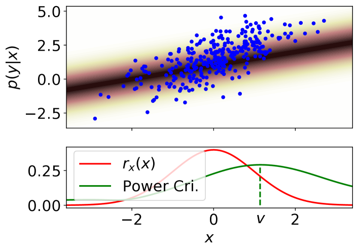
1. Illustration of the FSCD power criterion Our first task is to illustrate that the power criterion of the proposed FSCD test reveals where $p$ and $r$ differ in the domain of the conditioning variable ($\mathbf{x}$). We consider a simple univariate problem where the model is $p(y|x):=\mathcal{N}\left(x/2,1\right)$, the data generating distribution is $r(y|x):=\mathcal{N}(x,1)$, and $r_{x}(x)=\mathcal{N}(0,1)$. We use Gaussian kernels for both $k$ and $l$. The power criterion function is shown in Figure 1. More examples can be found in Section B (appendix).

Figure 1: The power criterion of FSCD as a function of $x$ is high where the difference between $p(y|x)$ and $r(y|x)$ can be best detected.

2. Test power

(a) Linear Gaussian Model ($H_{0}$)

(b) Hetero. Gaussian Model ($H_{1}$)

(c) Quadratic Gaussian Model ($H_{1}$)

Figure 2: Rejection rates of of the five tests with significance level $\alpha=0.05$. (a): $H_{0}$ is true. All test have false rejection rates no larger than $\alpha$ (up to sampling noise). (b): $H_{1}$ is true. FSCD-opt is good for detecting local difference. (c): KCSD is good for detecting global difference.

We investigate the test power of the following methods.

KCSD: our proposed KCSD test using Gaussian kernels $k(\mathbf{x},\mathbf{x}^{\prime})=\exp\left(-\frac{\|\mathbf{x}-\mathbf{x}^{\prime}\|^{2}}{2\sigma_{x}^{2}}\right)$ and $l(\mathbf{y},\mathbf{y}^{\prime})=\exp\left(-\frac{\|\mathbf{y}-\mathbf{y}^{\prime}\|^{2}}{2\sigma_{y}^{2}}\right)$ where the bandwidths are set with $\sigma_{x}:=\mathrm{median}\left(\left\{\|\mathbf{x}_{i}-\mathbf{x}_{j}\|_{2}\right\}_{i,j=1}^{n}\right)$ and $\sigma_{y}:=\mathrm{median}\left(\left\{\|\mathbf{y}_{i}-\mathbf{y}_{j}\|_{2}\right\}_{i,j=1}^{n}\right)$. This median heuristic has been used to set the bandwidth in many existing kernel-based tests (Gretton et al., 2012a; Bounliphone et al., 2015; Liu et al., 2016; Chwialkowski et al., 2016).

FSCD: our proposed FSCD test using Gaussian kernels for $k$ and $l$. There are two variations of the FSCD. In FSCD-rand, the $J$ test locations are randomly drawn from a Gaussian distribution fitted to the data with maximum likelihood. In the second variant FSCD-opt, 30% of the observed data are used for optimizing the two bandwidths and the $J$ test locations by maximizing the power criterion, and the rest 70% of the data are used for testing. All parameters of FSCD-opt are optimized jointly with Adam (Kingma and Ba, 2014) with default parameters implemented in Pytorch. We consider $J\in\{1,5\}$.

MMD: the Maximum Mean Discrepancy (MMD) test (Gretton et al., 2012a). The MMD test was originally created for two-sample testing. Here, we adapt it to conditional goodness-of-fit testing by splitting the data into two disjoint sets $\{(\mathbf{x}_{i}^{(1)},\mathbf{y}_{i}^{(1)})\}_{i=1}^{n/2}$ and $\{(\mathbf{x}_{i}^{(2)},\mathbf{y}_{i}^{(2)})\}_{i=1}^{n/2}\}$ of equal size $n/2$. We then sample $\mathbf{y}^{\prime}_{i}\sim p(\cdot|\mathbf{x}_{i}^{(2)})$ for each $i$. The test is performed on the first set, and $\{(\mathbf{x}_{i}^{(2)},\mathbf{y}_{i}^{\prime})\}_{i=1}^{n/2}$. The data splitting is performed to guarantee the independence between the two sets of samples, which is a requirement of the MMD test. We use the product of Gaussian kernels with bandwidths chosen by the median heuristic. This approach serves as a nonparametric baseline where the conditional model $p$ may be sampled easily.

Zheng: Zheng’s test (Zheng, 2012) is a specification test for parametric families of conditional distributions. It is based on an (average) squared difference between the empirical and the model CDFs, which is estimated by a U-statistic combined with a kernel density estimator. We found that Epanechnikov kernel suggested in (Zheng, 2012) resulted in a poor performance and therefore choose the standard Gaussian density as the smoothing kernel. We use a heuristic similar to (Zheng, 2012) to choose the kernel width parameters $h_{j}=\hat{s}_{{}_{j}}n^{-1/(12d_{x})}$, where $h_{j}$ is the bandwidth for the $j$-th coordinate of the covariate $\mathcal{\mathbf{x}}$, and $\hat{s}_{j}$ the standard deviation of the coordinate. The test requires the best fitting parameter in order to determine the fit of a given parametric family. Instead of a maximum likelihood estimator as proposed by Zheng (2012), in our experiments, the reference and the model distributions share the same parameter values, as the model family is a singleton set in our setting.

These methods are tested on the following problems:

Linear Gaussian Model (LGM): In this problem, $(\mathbf{x},y)\in\mathbb{R}^{5}\times\mathbb{R}$ and we set $p(y|\mathbf{x})=\mathcal{N}\left(\sum_{i=1}^{5}ix_{i},1\right)$, set $r:=p$ and $r_{x}(\mathbf{x})=\mathcal{N}(\mathbf{0},\mathbf{I})$. $H_{0}$ is true.

Heteroscedastic Gaussian Model (HGM): $(\mathbf{x},y)\in\mathbb{R}^{3}\times\mathbb{R}$ and $p(y|\mathbf{x})=\mathcal{N}\left(\sum_{i=1}^{3}x_{i},\sigma^{2}(\mathbf{x})\right)$ where $\sigma^{2}(\mathbf{x}):=1+10\exp\left(-\frac{\|\mathbf{x}-\mathbf{c}\|^{2}}{2\times 0.8^{2}}\right)$ and $\mathbf{c}=\frac{2}{3}\mathbf{1}$. We set the observation model to be $r(y|\mathbf{x})=\mathcal{N}\left(\sum_{i=1}^{3}x_{i},1\right)$ and set $r_{x}(\mathbf{x})=\mathcal{N}(\mathbf{0},\mathbf{I})$. In this problem, the observations are drawn from $r$ given by a linear Gaussian model with unit variance. The model $p$ is heteroscedastic (i.e., the noise depends on $\mathbf{x}$) where the variance function is created such that it is roughly 1 everywhere in the domain of $\mathbf{x}$, except in the region near $\mathbf{c}$. This problem is challenging since the difference is local in $\mathcal{X}$.

Quadratic Gaussian Model (QGM): $(x,y)\in\mathbb{R}\times\mathbb{R}$ and we define $p(y|x)=\mathcal{N}\left(x+1,1\right)$, $r\left(y|x\right)=\mathcal{N}\left(0.1x^{2}+x+1,1\right)$, and $r_{x}(x)=\mathrm{Uniform}\left(-2,2\right)$. Here, the conditional mean of the true distribution $r$ is given by a quadratic function, whereas the model $p$ is linear. This simulates a typical scenario where the model is too simplistic to model the data. Note that the quadratic term carries a small weight of 0.1, making the difference between $p$ and $r$ challenging to detect. In this case, $H_{1}$ is true.

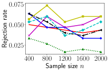
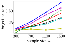
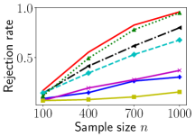
We report the rejection rates of these tests on all the three problems in Figure 2, where we conduct 300 independent trials for each experiment with the significance level set to $\alpha=0.05$. In Figure 2a, we observe that all the tests correctly have their false rejection rates no larger than $\alpha=0.05$ (up to sampling noise) since $H_{0}$ is true. In the HGM problem (Figure 2b) where the difference between $p$ and $r$ is local in the domain $\mathcal{X}$, we observe the optimized test locations of FSCD-opt are effective in identifying where to pinpoint to difference in $\mathcal{X}$. This can be seen by noting that the performance of FSCD-rand (random test locations) is significantly lower than FSCD-opt, since the test locations are randomized, and may be far from $\mathbf{c}$ which specifies the neighborhood that reveals the difference (see the specification of the HGM problem). While FSCD-opt has less test data since 30% of the data is spent on parameter tuning, the gain in the test power from having optimized test locations in the right region outweighs the small reduction of the test sample size.

In the QGM problem (Figure 2c), while the quadratic term in $r$ carries a small weight, as the sample size increases, all the power of all the tests increases as expected. We observe that the KCSD has higher performance than all variants of the FSCD in this case. This is because the difference between $p$ and $r$ is spatially diffuse in a manner that a pointwise evaluation of $\mathbf{v}\mapsto\|G_{p,r}(\mathbf{v})\|_{\mathcal{F}_{l}^{d_{y}}}^{2}$ (recall the FSCD statistic in (6)) is small everywhere in $\mathcal{X}=(-2,2)$. Thus, evaluating $G_{p,r}$ is less effective in this problem. In the case where the difference is spatially diffuse, it is more appropriate to take the norm of $G_{p,r}$, which explains the superior performance of the KCSD. We also note that in constrast to the HGM problem, in this case, FSCD-rand has higher performance than FSCD-opt because there is no particular region in $\mathcal{X}$ that gives higher signal than other. As a result, optimizing for test locations is less effective, and the test power drops because of smaller test sample size. Finally, we observe that in both HGM and QGM problems, the MMD has lower test power than other approaches due to the loss of information from representing a model $p$ with samples. Zheng’s test performs well in the QGM problem. Its statistic given by the expected squared difference between the empirical and the model CDFs can be seen as capturing global differences. However, its use of kernel density estimation may suffer when the data dimension is high as hinted in Figure 2a where it is overly conservative.

(a) Low power criterion
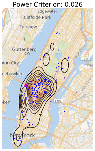
(relatively good fit)

(b) High power criterion
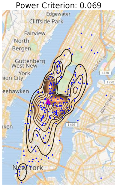
(relatively poor fit)

Figure 3: Mixture Density Network $p(\mathbf{y}|\mathbf{x})$ (black contour) trained on five million records in the NYC taxi dataset. Here, $\mathbf{y}$ is the drop-off location and $\mathbf{x}$ is the pick-up location. Blue points indicate real drop-off locations conditioned on the pick-up location at $\blacktriangle$ (shown in purple). The FSCD power criterion is evaluated at $J=1$ test location set to be at $\blacktriangle$. Since the model $p(\mathbf{y}|\mathbf{x}=\blacktriangle)$ fits less well in Figure 3b, the power criterion is larger than in Figure 3a.

3. Informative power criterion In our final experiment, we show with real data that the power criterion of the FSCD, as a function of $\mathbf{v}\in\mathcal{X}$ is a dimensionless quantity that roughly coincides with the degree of mismatch between $p(\mathbf{y}|\mathbf{v})$ and the data. We train a Mixture Density Network (MDN, Bishop (2006, Section 5.6)) on the New York City (NYC) taxi dataset. The dataset contains millions of trip records that include pick-up locations, drop-off locations, time, etc. The MDN models the conditional probability of the drop-off location $\mathbf{y}$ given a pick-up location $\mathbf{x}$, expressed as a latitude/longitude coordinate (i.e., $\mathcal{X},\mathcal{Y}\subset\mathbb{R}^{2}$). We train the model on five million trip records of yellow cabs from January 2015 using 20 Gaussian components, and a ReLU-based architecture for the mean, mixing proportion, and variance functions. For simplicity, only trips with pick-up and drop-off locations within or close to Manhattan are used.

We use Gaussian kernels for both $k$ and $l$ with their bandwidths chosen by the median heuristic, and separately compute the power criterion of the FSCD test at two manually chosen test locations, using a held-out data of size 12000. The results are shown in Figure 3 where blue points indicate observed drop-off locations conditioned on the pick-up location denoted by $\blacktriangle$. We consider conditioning separately on two pick-up locations $\blacktriangle_{1}$ and $\blacktriangle_{2}$, shown in Figure 3a and Figure 3b, respectively.

In Figure 3a, $p(\mathbf{y}|\mathbf{x}=\blacktriangle_{1})$ fits relatively well to the data compared to $p(\mathbf{y}|\mathbf{x}=\blacktriangle_{2})$ shown in 3b. In Figure 3b, the observed data (blue) do not respect the multimodality suggested by the model. As a result, the power criterion evaluated at $\blacktriangle_{2}$ is higher, indicating a poorer fit at $\blacktriangle_{2}$. This suggests that the power criterion function of the FSCD gives an interpretable indication for where the conditional model does not fit well. More details on the MDN and more results can be found in Section C (appendix).

6 CONCLUSION

We have proposed two novel conditional goodness-of-fit tests: the Kernel Conditional Stein Discrepancy (KCSD), and the Finite Set Conditional Discrepancy (FSCD). We prove that the population statistics of the two test define a proper divergence measure between two conditional density functions. There are several possible future directions. Both KCSD and FSCD can be extended to handle a discrete domain $\mathcal{Y}$ by considering a Stein operator defined in terms of forward and backward differences as in Yang et al. (2018). Further, our two tests can be sped up to have a runtime complexity linear in the sample size (instead of quadratic in the current version) by considering random Fourier features as in Huggins and Mackey (2018). The two tests can also be extended to compare the relative fit of two competing models as in Jitkrittum et al. (2018); Bounliphone et al. (2015). We leave these research directions for future work.

Acknowledgment

We thank Patsorn Sangkloy for helping us with the experiment on the NYC taxi dataset. HK thanks the Gatsby Charitable Foundation for the financial support

Appendix A PROOFS

This section contains proofs of the theoretical results we gave in the main text. We first give two known lemmas that will be needed.

Lemma 7 (Carmeli et al., 2008, Theorem 2b, Section 4 (rephrased)).

Let $\mathcal{X}$ be a locally compact second countable topological space, and $\mathcal{Z}$ be a complex separable Hilbert space. Let $K\colon\mathcal{X}\times\mathcal{X}\to\mathcal{L}(\mathcal{Z})$ be a $C_{0}$ universal kernel associated with the vector-valued RKHS $\mathcal{F}_{K}$, where $\mathcal{L}(\mathcal{Z})$ denotes the Banach space of bounded operators from $\mathcal{Z}$ to $\mathcal{Z}$. Let $P$ be a probability measure on $\mathcal{X}$. Then, the operator $L_{P}\colon L^{2}(\mathcal{X},P;\mathcal{Z})\rightarrow\mathcal{F}_{K}$ given by $(L_{P}f)(\mathbf{t})=\int_{\mathcal{X}}K(\mathbf{t},\mathbf{x})f(\mathbf{x})\thinspace\mathrm{d}P(\mathbf{x})$ is injective, for all $f\in L^{2}(\mathcal{X},P;\mathcal{Z})$.

Lemma 8 (Chwialkowski et al. 2015, Lemma 1).

If $k\colon\mathbb{R}^{d_{x}}\times\mathbb{R}^{d_{x}}\to\mathbb{R}$ is a bounded, real analytic kernel (i.e., for any $\mathbf{v}\in\mathcal{X}$, $\mathbf{x}\mapsto k(\mathbf{x},\mathbf{v})$ is a real analytic function), then all functions in the RKHS defined by $k$ are real analytic.

A.1 PROOF OF THEOREM 1

Recall the theorem: See 1

Proof.

We first rewrite the statistic as

$$D_{p}^{2}(r) =\big{\|}\mathbb{E}_{(\mathbf{x},\mathbf{y})\sim r_{xy}}K_{\mathbf{x}}\xi_{p_{|\mathbf{x}}}(\mathbf{y},\diamond)\big{\|}_{\mathcal{F}_{K}}^{2}$$

$$=\big{\|}\mathbb{E}_{\mathbf{x}\sim r_{x}}K_{\mathbf{x}}\mathbb{E}_{\mathbf{y}\sim r_{|\mathbf{x}}}\xi_{p_{|\mathbf{x}}}(\mathbf{y},\diamond)\big{\|}_{\mathcal{F}_{K}}^{2}$$

$$=\big{\|}\mathbb{E}_{\mathbf{x}\sim r_{x}}K_{\mathbf{x}}\mathbf{g}_{p,r}(\diamond|\mathbf{x})\big{\|}_{\mathcal{F}_{K}}^{2},$$

where $\mathbf{g}_{p,r}(\mathbf{w}|\mathbf{x}):=\mathbb{E}_{\mathbf{y}\sim r_{|\mathbf{x}}}\xi_{p_{|\mathbf{x}}}(\mathbf{y},\mathbf{w})\in\mathbb{R}^{d_{y}}$ is the Stein witness function between $p_{|\mathbf{x}}$ and $r_{|\mathbf{x}}$, and $\xi_{p_{|\mathbf{x}}}(\mathbf{y},\cdot):=l(\mathbf{y},\cdot)\nabla_{\mathbf{y}}\log p(\mathbf{y}|\mathbf{x})+\nabla_{\mathbf{y}}l(\mathbf{y},\cdot)\in\mathcal{F}_{l}^{d_{y}}$ for $r_{x}$-almost all $\mathbf{x}$ (Chwialkowski et al., 2016; Liu et al., 2016; Jitkrittum et al., 2017b). By Chwialkowski et al. (2016, Theorem 2.2), for $r_{x}$-almost all $\mathbf{x}\in\mathcal{X}$, the Kernel Stein Discrepancy (KSD) between the two probability density functions $p_{|\mathbf{x}}$ and $r_{|\mathbf{x}}$ is 0 if and only if they coincide. That is, given $\mathbf{x}\sim r_{x}$, $\mathrm{KSD}_{p_{|\mathbf{x}}}^{2}(r_{|\mathbf{x}})=0=\|\mathbf{g}_{p,r}(\diamond|\mathbf{x})\|_{\mathcal{F}_{l}^{d_{y}}}^{2}$ if and only if $p_{|\mathbf{x}}=r_{|\mathbf{x}}$. Thus, proving the claim amounts to showing $\mathbf{g}_{p,r}(\diamond|\mathbf{x})=\mathbf{0}$ for $r_{x}$-almost all $\mathbf{x}$ if and only if $p\stackrel{{\scriptstyle r_{x}}}{{=}}r$. Since $\mathbf{g}_{p,r}\in L^{2}(\mathcal{X},r_{x};\mathcal{F}_{l}^{d_{y}})$ and $K$ is $C_{0}$-universal, Lemma 7 (by setting $\mathcal{Z}=\mathcal{F}_{l}^{d_{y}}$) implies that the map $\mathbf{g}_{p,r}\mapsto\mathbb{E}_{\mathbf{x}\sim r_{x}}K_{\mathbf{x}}\mathbf{g}_{p,r}(\diamond|\mathbf{x})$ is injective. As a result of the injectivity and the fact that $A\mathbf{0}=\mathbf{0}$ if $A$ is a linear operator, we have $\mathbb{E}_{\mathbf{x}\sim r_{x}}K_{\mathbf{x}}\mathbf{g}_{p,r}(\diamond|\mathbf{x})=\mathbf{0}$ if and only if $\mathbf{g}_{p,r}=\mathbf{0}$ or equivalently $\mathbf{g}_{p,r}(\diamond|\mathbf{x})=\mathbf{0}$ for all $r_{x}$-almost all $\mathbf{x}$. ∎

A.2 PROOF OF PROPOSITION 2

From (2), we have

$$D_{p}(r) =\big{\|}\mathbb{E}_{(\mathbf{x},\mathbf{y})\sim r_{xy}}K_{\mathbf{x}}\xi_{p_{|\mathbf{x}}}(\mathbf{y},\diamond)\big{\|}_{\mathcal{F}_{K}}^{2}$$

$$=\left\langle\mathbb{E}_{\mathbf{xy}}K_{\mathbf{x}}\xi_{p_{|\mathbf{x}}}(\mathbf{y},\diamond),\mathbb{E}_{\mathbf{x^{\prime}y^{\prime}}}K_{\mathbf{x^{\prime}}}\xi_{p_{|\mathbf{x}^{\prime}}}(\mathbf{y}^{\prime},\diamond)\right\rangle_{\mathcal{F}_{K}}$$

$$\stackrel{{\scriptstyle(a)}}{{=}}\mathbb{E}_{\mathbf{xy}}\mathbb{E}_{\mathbf{x^{\prime}y^{\prime}}}\left\langle K_{\mathbf{x}}\xi_{p_{|\mathbf{x}}}(\mathbf{y},\diamond),K_{\mathbf{x^{\prime}}}\xi_{p_{|\mathbf{x}^{\prime}}}(\mathbf{y}^{\prime},\diamond)\right\rangle_{\mathcal{F}_{K}}$$

$$\stackrel{{\scriptstyle(b)}}{{=}}\mathbb{E}_{\mathbf{xy}}\mathbb{E}_{\mathbf{x^{\prime}y^{\prime}}}\left\langle K_{\mathbf{x}^{\prime}}^{*}K_{\mathbf{x}}\xi_{p_{|\mathbf{x}}}(\mathbf{y},\diamond),\xi_{p_{|\mathbf{x}^{\prime}}}(\mathbf{y}^{\prime},\diamond)\right\rangle_{\mathcal{F}_{l}^{d_{y}}}$$

$$=\mathbb{E}_{\mathbf{xy}}\mathbb{E}_{\mathbf{x^{\prime}y^{\prime}}}k(\mathbf{x},\mathbf{x}^{\prime})h_{p}((\mathbf{x},\mathbf{y}),(\mathbf{x}^{\prime},\mathbf{y}^{\prime})),$$

where at $(a)$ the expectation and the inner product commute because of Bochner integrability of $(\mathbf{x},\mathbf{y})\mapsto K_{\mathbf{x}}\xi_{p_{|\mathbf{x}}}(\mathbf{y},\diamond)$ (see assumption 4 in Theorem 1, and Steinwart and Christmann (2008, Definition A.5.20)), at $(b)$ we use the adjoint $K_{\mathbf{x}^{\prime}}^{*}$ and the reproducing property i.e., $K_{\mathbf{x}^{\prime}}^{*}K_{\mathbf{x}}=K(\mathbf{x},\mathbf{x}^{\prime})=k(\mathbf{x},\mathbf{x}^{\prime})I$,

$$h_{p}((\mathbf{x},\mathbf{y}),(\mathbf{x}^{\prime},\mathbf{y}^{\prime})):=\left\langle\xi_{p_{|\mathbf{x}}}(\mathbf{y},\diamond),\xi_{p_{|\mathbf{x}^{\prime}}}(\mathbf{y}^{\prime},\diamond)\right\rangle_{\mathcal{F}_{l}^{d_{y}}}$$

$$=l(\mathbf{y},\mathbf{y}^{\prime})\mathbf{s}_{p}^{\top}(\mathbf{y}|\mathbf{x})\mathbf{s}_{p}(\mathbf{y}^{\prime}|\mathbf{x}^{\prime})+\sum_{i=1}^{d_{y}}\frac{\partial^{2}}{\partial y_{i}\partial y_{i}^{\prime}}l(\mathbf{y},\mathbf{y}^{\prime})$$

$$\phantom{=}+\mathbf{s}_{p}^{\top}(\mathbf{y}|\mathbf{x})\nabla_{\mathbf{y}^{\prime}}l(\mathbf{y},\mathbf{y}^{\prime})+\mathbf{s}_{p}^{\top}(\mathbf{y}^{\prime}|\mathbf{x}^{\prime})\nabla_{\mathbf{y}}l(\mathbf{y},\mathbf{y}^{\prime}),$$

and $\mathbf{s}_{p}(\mathbf{y}|\mathbf{x}):=\nabla_{\mathbf{y}}\log p(\mathbf{y}|\mathbf{x})$.

A.3 PROOF OF PROPOSITION 3

Define $\zeta_{1}:=\mathbb{V}\left[\mathbb{E}_{(\mathbf{x},\mathbf{y})\sim r_{xy}}H_{p}((\mathbf{x},\mathbf{y}),(\mathbf{x}^{\prime},\mathbf{y}^{\prime}))\right]$. We only need to show that under $H_{0}$, $\widehat{D_{p}}$ is a degenerate U-statistic i.e., $\zeta_{1}=0$, and under $H_{1}$, $\widehat{D_{p}}$ is non-degenerate i.e., $\zeta_{1}>0$. Then, the asymptotic distributions in the two cases follow from Serfling (2009, Section 5.5).

Case: $H_{0}$ is true

$$\mathbb{E}_{(\mathbf{x},\mathbf{y})\sim r_{xy}}H_{p}((\mathbf{x},\mathbf{y}),(\mathbf{x}^{\prime},\mathbf{y}^{\prime})) =\mathbb{E}_{(\mathbf{x},\mathbf{y})\sim r_{xy}}\left\langle K_{\mathbf{x}}\xi_{p_{|\mathbf{x}}}(\mathbf{y},\diamond),K_{\mathbf{x^{\prime}}}\xi_{p_{|\mathbf{x}^{\prime}}}(\mathbf{y}^{\prime},\diamond)\right\rangle_{\mathcal{F}_{K}}$$

$$\stackrel{{\scriptstyle(a)}}{{=}}\left\langle\mathbb{E}_{(\mathbf{x},\mathbf{y})\sim r_{xy}}K_{\mathbf{x}}\xi_{p_{|\mathbf{x}}}(\mathbf{y},\diamond),K_{\mathbf{x^{\prime}}}\xi_{p_{|\mathbf{x}^{\prime}}}(\mathbf{y}^{\prime},\diamond)\right\rangle_{\mathcal{F}_{K}},$$ (8)

where the interchange of the inner product and the expectation is justified since $\mathbb{E}_{\mathbf{xy}}\|K_{\mathbf{x}}\xi_{p_{|\mathbf{x}}}(\mathbf{y},\diamond)\|_{\mathcal{F}_{K}}<\infty$ (Bochner integrability). But by Theorem 1 and (2), we have that $G_{p,r}:=\mathbb{E}_{(\mathbf{x},\mathbf{y})\sim r_{xy}}K_{\mathbf{x}}\xi_{p_{|\mathbf{x}}}(\mathbf{y},\diamond)=\mathbf{0}$. So, $\zeta_{1}=0$ and the result under $H_{0}$ follows from Serfling (2009, Section 5.5.2).

Case: $H_{1}$ is true

From (3), it can be seen that

$$\eqref{eq:kssd_half_eval_ustat} =\mathbb{E}_{\mathbf{xy}}k(\mathbf{x},\mathbf{x}^{\prime})h_{p}((\mathbf{x},\mathbf{y}),(\mathbf{x}^{\prime},\mathbf{y}^{\prime})):=t(\mathbf{x}^{\prime},\mathbf{y}^{\prime}).$$

Since $\zeta_{1}=\mathbb{V}[t(\mathbf{x},\mathbf{y})]$, it suffices to show that $t$ is not a constant function. To see this, note that the kernel $k$ is $C_{0}$-universal and cannot be a constant function. The function $h_{p}$ (see (4)) includes the kernel $l$ which is also $C_{0}$-universal. Therefore, $t$ is not a constant function and $\zeta_{1}>0$. We get the asymptotic normality from the result in Serfling (2009, Section 5.5.1).

A.4 PROOF OF THEOREM 4

Recall the proposition from the main text:See 4

Proof.

Recall that $T_{p}^{V}(r):=\frac{1}{Jd_{y}}\sum_{i=1}^{J}\|G_{p,r}(\mathbf{v}_{i})\|_{\mathcal{F}_{l}^{d_{y}}}^{2}.$ If $H_{0}$ is true, then $G_{p,r}=\mathbf{0}$ by Theorem 1. As a result, $T_{p}^{V}(r)=0$. Now suppose that $H_{1}$ is true. We first show that $\tilde{G}(\mathbf{v}):=\|G_{p,r}(\mathbf{v})\|_{\mathcal{F}_{l}^{d_{y}}}^{2}$ is a real analytic function. Consider

$$\bar{G}(\mathbf{v},\mathbf{v^{\prime}}) =\mathbb{E}_{\mathbf{x}\mathbf{y}}\mathbb{E}_{\mathbf{x^{\prime}y^{\prime}}}k(\mathbf{x},\mathbf{v})k(\mathbf{x}^{\prime},\mathbf{v}^{\prime})h_{p}((\mathbf{x},\mathbf{y}),(\mathbf{x}^{\prime},\mathbf{y}^{\prime}))$$

$$=\mathbb{E}_{\mathbf{x,x^{\prime}}}\tilde{k}[(\mathbf{x},\mathbf{x}^{\prime}),(\mathbf{v},\mathbf{v}^{\prime})]\tilde{h}_{p}(\mathbf{x},\mathbf{x}^{\prime}),$$

where $\tilde{k}[(\mathbf{x},\mathbf{x}^{\prime}),(\mathbf{v},\mathbf{v}^{\prime})]:=k(\mathbf{x},\mathbf{v})k(\mathbf{x}^{\prime},\mathbf{v}^{\prime})$ and $\tilde{h}_{p}(\mathbf{x},\mathbf{x^{\prime}})=\mathbf{\mathbb{E}_{y|\mathbf{x}}\mathbb{E}_{\mathbf{y^{\prime}}|\mathbf{x^{\prime}}}}h_{p}((\mathbf{x},\mathbf{y}),(\mathbf{x}^{\prime},\mathbf{y}^{\prime}))$. Note that $\tilde{h}_{p}(\mathbf{x},\mathbf{x}^{\prime})=\langle\mathbf{g}_{p,r}(\diamond|\mathbf{x}),\mathbf{g}_{p,r}(\diamond|\mathbf{x}^{\prime})\rangle_{\mathcal{F}_{l}^{d_{y}}}$, and thus we have

$$\mathbb{E}_{\mathbf{x,x^{\prime}}} \langle\mathbf{g}_{p,r}(\diamond|\mathbf{x}),\mathbf{g}_{p,r}(\diamond|\mathbf{x}^{\prime})\rangle_{\mathcal{F}_{l}^{d_{y}}}^{2}\leq\left(\mathbf{\mathbb{E}_{\mathbb{\mathbf{x}}}}\lVert\mathbf{g}_{p,r}(\diamond|\mathbf{x})\rVert_{\mathcal{F}_{l}^{d_{y}}}^{2}\right)^{2}.$$

The RHS is finite by Assumption 3 in Theorem 1, and so $\tilde{h}_{p}\in L^{2}(\mathcal{X\times\mathcal{X}},r_{x}\otimes r_{x})$. Therefore, $\bar{G}$ is given by the integral transform of $\tilde{h}_{p}$ with respect to the kernel $\tilde{k}$, which implies that $\bar{G}$ is an element of the RKHS of $\tilde{k}$ (Steinwart and Christmann, 2008, Theorem 4.26). Since the product of real analytic functions is real analytic, consequently for any $(\mathbf{v},\mathbf{v}^{\prime})$, $(\mathbf{z},\mathbf{z}^{\prime})\mapsto\tilde{k}[\mathbf{(z},\mathbf{z}^{\prime}),\mathbf{(v,\mathbf{v^{\prime})}}]$ is real analytic and bounded by our assumption. Thus, by Lemma 8, $\bar{G}(\mathbf{v},\mathbf{v}^{\prime})$ is analytic. From (9), we have $\tilde{G}(\mathbb{\mathbf{v}})=\bar{G}(\mathbf{v},\mathbf{v})$; hence $\tilde{G}$ is analytic and not a zero function by Theorem 1. Since the zero set of $\tilde{G}(\mathbf{v})$, $\{\mathbf{v}^{\prime}\in\mathcal{X}\mid\tilde{G}(\mathbf{v}^{\prime})=0\}$, has zero Lebesgue measure (Mityagin, 2015), we have that $\eta$-almost surely $\tilde{G}(\mathbf{v})>0$ for any $\mathbf{v}\sim\eta$, and the result follows. ∎

A.5 PROOF OF PROPOSITION 5

From (6), we first rewrite $\|G_{p,r}(\mathbf{v})\|_{\mathcal{F}_{l}^{d_{y}}}^{2}$ as

$$\|G_{p,r}(\mathbf{v})\|_{\mathcal{F}_{l}^{d_{y}}}^{2}=\big{\|}\left[\mathbb{E}_{(\mathbf{x},\mathbf{y})\sim r_{xy}}K_{\mathbf{x}}\xi_{p_{|\mathbf{x}}}(\mathbf{y},\diamond)\right](\mathbf{v})\big{\|}_{\mathcal{F}_{l}^{d_{y}}}^{2}$$

$$\stackrel{{\scriptstyle(a)}}{{=}}\big{\|}\mathbb{E}_{(\mathbf{x},\mathbf{y})\sim r_{xy}}K(\mathbf{x},\mathbf{v})\xi_{p_{|\mathbf{x}}}(\mathbf{y},\diamond)\big{\|}_{\mathcal{F}_{l}^{d_{y}}}^{2}$$

$$\stackrel{{\scriptstyle(b)}}{{=}}\mathbb{E}_{\mathbf{x}\mathbf{y}}\mathbb{E}_{\mathbf{x^{\prime}y^{\prime}}}k(\mathbf{x},\mathbf{v})k(\mathbf{x}^{\prime},\mathbf{v})h_{p}((\mathbf{x},\mathbf{y}),(\mathbf{x}^{\prime},\mathbf{y}^{\prime}))$$ (9)

where at $(a)$ we use $(K_{\mathbf{x}}f)(\mathbf{v})=K(\mathbf{x},\mathbf{v})f$ for $f\in\mathcal{F}_{l}^{d_{y}}$, and at $(b)$ we use $h_{p}((\mathbf{x},\mathbf{y}),(\mathbf{x}^{\prime},\mathbf{y}^{\prime}))=\left\langle\xi_{p_{|\mathbf{x}}}(\mathbf{y},\diamond),\xi_{p_{|\mathbf{x}^{\prime}}}(\mathbf{y}^{\prime},\diamond)\right\rangle_{\mathcal{F}_{l}^{d_{y}}}$ as in (3). It follows from (6) that

$$T_{p}^{V}(r) =\mathbb{E}_{\mathbf{x}\mathbf{y}}\mathbb{E}_{\mathbf{x^{\prime}y^{\prime}}}\overline{H}_{p}^{V}((\mathbf{x},\mathbf{y}),(\mathbf{x}^{\prime},\mathbf{y}^{\prime})),$$

where $(\mathbf{x},\mathbf{y}),(\mathbf{x}^{\prime},\mathbf{y}^{\prime})$ are i.i.d. random variables following $r_{xy}$,

$$\overline{H}_{p}^{V}((\mathbf{x},\mathbf{y}),(\mathbf{x}^{\prime},\mathbf{y}^{\prime})):=\frac{1}{d_{y}}\overline{k}_{V}(\mathbf{x},\mathbf{x}^{\prime})h_{p}((\mathbf{x},\mathbf{y}),(\mathbf{x}^{\prime},\mathbf{y}^{\prime})),$$

and $\overline{k}_{V}(\mathbf{x},\mathbf{x}^{\prime}):=\frac{1}{J}\sum_{i=1}^{J}k(\mathbf{x},\mathbf{v}_{i})k(\mathbf{x}^{\prime},\mathbf{v}_{i})$ is a kernel that depends on $V$.

Proposition 9 (Asymptotic distributions of $\widehat{T_{p}^{V}}$).

Assume that $\mathbb{E}\overline{k}_{V}^{2}(\mathbf{x},\mathbf{x}^{\prime})h_{p}^{2}((\mathbf{x},\mathbf{y}),(\mathbf{x}^{\prime},\mathbf{y}^{\prime}))<\infty$. The following statements hold.

1. If $\sigma_{V}^{2}:=4\mathbb{V}[\mathbb{E}_{\mathbf{xy}}[\overline{H}_{p}^{V}((\mathbf{x},\mathbf{y}),(\mathbf{x}^{\prime},\mathbf{y}^{\prime}))]]>0$, then $\sqrt{n}\left(\widehat{T_{p}^{V}}-T_{p}^{V}(r)\right)\stackrel{{\scriptstyle d}}{{\to}}\mathcal{N}(0,\sigma_{V}^{2})$;

2. If $\sigma_{V}^{2}=0$, then $n\widehat{T_{p}^{V}}\stackrel{{\scriptstyle d}}{{\to}}\sum_{j=1}^{\infty}\lambda_{j}(\chi_{1j}^{2}-1)$, where $\{\chi_{1j}^{2}\}_{j}$ are independent $\chi_{1}^{2}$ random variables, $\lambda_{j}$ are eigenvalues of the operator $A$ defined as $(A\varphi)(\mathbf{z})=\int\overline{H}_{p}^{V}(\mathbf{z},\mathbf{z}^{\prime})\varphi(\mathbf{z}^{\prime})r_{xy}(\mathbf{z}^{\prime})\thinspace\mathrm{d}\mathbf{z}^{\prime}$ for non-zero $\varphi$, $\mathbf{z}:=(\mathbf{x},\mathbf{y})$ and $\mathbf{z}^{\prime}:=(\mathbf{x}^{\prime},\mathbf{y}^{\prime})$.

Appendix B ILLUSTRATION OF THE FSCD POWER CRITERION

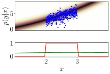
To complement Figure 1, in this section, we illustrate the behavior of the power criterion of the FSCD as a function of the test location on a number of one-dimensional problems. These are shown in Figure 4 where observed data from $r$ are shown in blue. In all cases, the two kernels $k$ and $l$ are set to Gaussian kernels.

(a) Quadratic Gaussian Model (Gaussian $r_{x}$)

(b) Hetero. Gaussian Model

(c) Quadratic Gaussian Model (uniform $r_{x}$)

Figure 4: The power criterion as a function of $x$ on a number of synthetic one-dimensional problems.

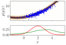
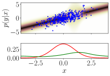
In Figure 4a, $p(y|x):=\mathcal{N}\left(x+0.5x^{2}-1,1\right),r(y|x):=\mathcal{N}\left(x+0.4x^{2}-1,1\right),$ and $r_{x}(x):=\mathcal{N}(2,1)$. Here, the difference between the data generating distribution $r$ and the model $p$ is the in the coefficients of the second-order term in the mean, which differ only slightly. We observe that the power criterion function is non-zero almost everywhere.

In Figure 4b, $p(y|x):=\mathcal{N}\left(x,\sigma^{2}(x)\right)$ where the variance function is $\sigma^{2}(x):=1+8\exp\left(-\frac{(x-1)^{2}}{2\times 0.3^{2}}\right)$. This is a linear regression model with heteroscedastic noise, and is similar to the HGM model considered in Section 5. We set $r(y|x):=\mathcal{N}(x,1)$ and $r_{x}(x):=\mathcal{N}(0,1)$. The problem is designed so that the model and the true conditional density have the same (conditional) mean, but differ locally in the conditional variance i.e., at $x=1$. We observe that the power criterion function indeed has a peak around $x=1$, indicating that it is sensitive to local differences. Note that theoretically the power criterion function is non-zero almost everywhere (but could be arbitrarily close to zero).

In Figure 4c, we consider the same $p$ and $r$ as specified in Figure 4a, but change $r_{x}$ to be a uniform distribution defined on $[2,3]$. Since $p$ is different from $r$, the power criterion function is non-zero almost everywhere (implied by Theorem 4), and this is indeed the case. We note that this statement holds true regardless of $r_{x}$, as evident in Figure 4c (cf. Figure 4a). In particular, the support of $r_{x}$ may not cover the whole domain $\mathcal{X}$.

Appendix C NYC TAXI DATA EXPERIMENT

C.1 TRAINING OF THE MIXTURE DENSITY NETWORK

Here, we describe technical details of the Mixture Density Network (MDN) used in the NYC taxi data experiment for estimating the conditional probability of a drop-off location given a pick-up location. The NYC taxi dataset is available at https://www1.nyc.gov/site/tlc/about/tlc-trip-record-data.page. An MDN specifies a conditional density model of the form

$$p(\mathbf{y}|\mathbf{x}) =\sum_{i=1}^{C}\pi_{i}(\mathbf{x})\mathcal{N}\left(\mathbf{y}\mid\bm{\mu}_{i}(\mathbf{x}),\mathrm{diag}\left(\sigma_{i,1}^{2}(\mathbf{x}),\ldots,\sigma_{i,d_{y}}^{2}(\mathbf{x})\right)\right),$$

where $C$ is the number of Gaussian components, $\mathbf{x}\in\mathbb{R}^{d_{x}},\mathbf{y}\in\mathbb{R}^{d_{y}}$ and $\mathrm{diag}(\mathbf{s})$ constructs a diagonal matrix with the diagonal entries given by $\mathbf{v}$. In our problem, $\mathbf{x}$ (pick-up location) and $\mathbf{y}$ (drop-off location) contain latitude/longitude coordinates; so, $d_{x}=d_{x}=2$. The mixing proportion function $\bm{\pi}(\mathbf{x}):=(\pi_{1}(\mathbf{x}),\ldots,\pi_{C}(\mathbf{x}))$, the mean function $\bm{\mu}(\mathbf{x}):=(\bm{\mu}_{1}(\mathbf{x}),\ldots,\bm{\mu}_{C}(\mathbf{x}))^{\top}\in\mathbb{R}^{C\times d_{y}}$, and the variance function $\bm{\sigma}^{2}(\mathbf{x}):=\left(\sigma_{i,j}^{2}(\mathbf{x})\right)_{i,j}\in\mathbb{R}_{+}^{C\times d_{y}}$ for $i\in\{1,\ldots,C\},j\in\{1,2\}$ depend on $\mathbf{x}$ and are specified by neural networks. The network architecture is as follows:

Layer $\downarrow$	Input	Output
Linear	$d_{x}=2$	128
Batch normalization	-	-
ReLU activation	-	-
Linear	128	64
Batch normalization	-	-
ReLU activation	-	-
Linear	64	$C=20$
Softmax	-	-

tableNetwork architecture for $\bm{\pi}$.

Layer $\downarrow$	Input	Output
Linear	$d_{x}=2$	128
Batch normalization	-	-
ReLU activation	-	-
Linear	128	64
Batch normalization	-	-
Linear	64	$C\times d_{y}$

tableNetwork architecture for $\bm{\mu}$.

Layer $\downarrow$	Input	Output
Linear	$d_{x}=2$	128
Batch normalization	-	-
ReLU activation	-	-
Linear	128	64
Batch normalization	-	-
Linear	64	$C\times d_{y}$

tableNetwork architecture for $\bm{\sigma}^{2}$.

We train the model on five million trip records of New York’s yellow cabs from January 2015 using $C=20$ Gaussian components. Only trips with pick-up and drop-off locations within or close to Manhattan are used. The training objective function is the negative log likelihood. We train the model for three epochs using Adam (Kingma and Ba, 2014) as the optimization procedure, with a minibatch size of 2000, and a learning rate of 0.001.

C.2 POWER CRITERION OF THE FSCD

In this section, we show more results akin to Figure 3. Here, we sample a number of candidate test location $\mathbf{v}$’s, and evaluate the FSCD power criterion (see Section 4.2) at each of these locations separately. The test location is denoted by $\blacktriangle$ in the following figures. We use the same setting as used to produce Figure 3. It is worth reiterating that the same sample $\{(\mathbf{x}_{i},\mathbf{y}_{i})\}_{i=1}^{12000}$ is used to compute the power criterion in all cases. Each of the following figures corresponds to one realization of $\mathbf{v}$. Only sample points $\{(\mathbf{x}_{i},\mathbf{y}_{i})\mid i=1,\ldots,12000\text{ and }\mathbf{x}_{i}\text{ is close to }\text{{v }}\}$ are shown (in blue), and not the full sample. The trained MDN’s density function $p(\cdot|\mathbf{v})$ is shown as a contour plot (in black).

We observe that the power criterion (dimensionless quantity) roughly corresponds to the degree of mismatch between the conditional model $p(\cdot|\mathbf{v})$ and the observed data i.e., high when the mismatch is large. We note that power criterion values are affected by the choice of the two kernels $k,l$, quality of the trained model, and the sample size used to compute the power criterion. Changing the two kernels may (and likely will) change the values of the power criterion, and the ordering of these cases. Thoroughly studying the effects of these factors on the computed power criterion will be an interesting topic of future research.

References

- Andrews (1997) D. W. K. Andrews. A conditional Kolmogorov test. Econometrica, 65(5):1097–1128, 1997.
- Arcones and Gine (1992) M. A. Arcones and E. Gine. On the bootstrap of U and V statistics. The Annals of Statistics, pages 655–674, 1992.
- Berlinet and Thomas-Agnan (2011) A. Berlinet and C. Thomas-Agnan. Reproducing kernel Hilbert spaces in probability and statistics. Springer Science & Business Media, 2011.
- Bierens (1982) H. J. Bierens. Consistent model specification tests. Journal of Econometrics, 20(1):105 – 134, 1982. ISSN 0304-4076.
- Bierens (1990) H. J. Bierens. A consistent conditional moment test of functional form. Econometrica: Journal of the Econometric Society, pages 1443–1458, 1990.
- Bierens and Ploberger (1997) H. J. Bierens and W. Ploberger. Asymptotic theory of integrated conditional moment tests. Econometrica: Journal of the Econometric Society, pages 1129–1151, 1997.
- Bishop (2006) C. M. Bishop. Pattern recognition and machine learning. Springer, 2006.
- Bounliphone et al. (2015) W. Bounliphone, E. Belilovsky, M. B. Blaschko, I. Antonoglou, and A. Gretton. A test of relative similarity for model selection in generative models. In ICLR, 2015.
- Carmeli et al. (2008) C. Carmeli, E. De Vito, A. Toigo, and V. Umanità. Vector valued reproducing kernel Hilbert spaces and universality. arXiv e-prints, Jul 2008.
- Carmeli et al. (2006) C. Carmeli, E. De Vito, and A. Toigo. Vector valued reproducing kernel Hilbert spaces of integrable functions and Mercer theorem. Analysis and Applications, 4(04):377–408, 2006.
- Chwialkowski et al. (2015) K. Chwialkowski, A. Ramdas, D. Sejdinovic, and A. Gretton. Fast two-sample testing with analytic representations of probability measures. In Advances in Neural Information Processing Systems, pages 1981–1989, 2015.
- Chwialkowski et al. (2016) K. Chwialkowski, H. Strathmann, and A. Gretton. A kernel test of goodness of fit. In ICML, pages 2606–2615, 2016.
- Dutordoir et al. (2018) V. Dutordoir, H. Salimbeni, J. Hensman, and M. Deisenroth. Gaussian process conditional density estimation. In NeurIPS, pages 2385–2395, 2018.
- Gorham and Mackey (2017) J. Gorham and L. Mackey. Measuring sample quality with kernels. In ICML, pages 1292–1301, 2017.
- Gretton et al. (2008) A. Gretton, K. Fukumizu, C. H. Teo, L. Song, B. Schölkopf, and A. J. Smola. A kernel statistical test of independence. In NeurIPS, pages 585–592, 2008.
- Gretton et al. (2009) A. Gretton, K. Fukumizu, Z. Harchaoui, and B. K. Sriperumbudur. A fast, consistent kernel two-sample test. In NeurIPS, pages 673–681. 2009.
- Gretton et al. (2012a) A. Gretton, K. M. Borgwardt, M. J. Rasch, B. Schölkopf, and A. Smola. A kernel two-sample test. Journal of Machine Learning Research, 13:723–773, 2012a.
- Gretton et al. (2012b) A. Gretton, D. Sejdinovic, H. Strathmann, S. Balakrishnan, M. Pontil, K. Fukumizu, and B. K. Sriperumbudur. Optimal kernel choice for large-scale two-sample tests. In NeurIPS, pages 1205–1213, 2012b.
- Huggins and Mackey (2018) J. Huggins and L. Mackey. Random feature Stein discrepancies. In NeurIPS, pages 1899–1909, 2018.
- Huskova and Janssen (1993) M. Huskova and P. Janssen. Consistency of the generalized bootstrap for degenerate -statistics. Ann. Statist., 21(4):1811–1823, 12 1993.
- Jitkrittum et al. (2016) W. Jitkrittum, Z. Szabó, K. P. Chwialkowski, and A. Gretton. Interpretable distribution features with maximum testing power. In NeurIPS, pages 181–189. 2016.
- Jitkrittum et al. (2017a) W. Jitkrittum, Z. Szabó, and A. Gretton. An adaptive test of independence with analytic kernel embeddings. In ICML. 2017a.
- Jitkrittum et al. (2017b) W. Jitkrittum, W. Xu, Z. Szabo, K. Fukumizu, and A. Gretton. A linear-time kernel goodness-of-fit test. In NeurIPS, 2017b.
- Jitkrittum et al. (2018) W. Jitkrittum, H. Kanagawa, P. Sangkloy, J. Hays, B. Schölkopf, and A. Gretton. Informative features for model comparison. In NeurIPS, pages 808–819, 2018.
- Kingma and Ba (2014) D. P. Kingma and J. Ba. Adam: A method for stochastic optimization. arXiv preprint arXiv:1412.6980, 2014.
- Liu et al. (2016) Q. Liu, J. Lee, and M. Jordan. A kernelized Stein discrepancy for goodness-of-fit tests. In ICML, pages 276–284, 2016.
- Mityagin (2015) B. Mityagin. The zero set of a real analytic function. arXiv e-prints, art. arXiv:1512.07276, Dec 2015.
- Moreira (2003) M. J. Moreira. A conditional likelihood ratio test for structural models. Econometrica, 71(4):1027–1048, 2003.
- Oates et al. (2017) C. J. Oates, M. Girolami, and N. Chopin. Control functionals for Monte Carlo integration. Journal of the Royal Statistical Society: Series B (Statistical Methodology), 79(3):695–718, 2017. doi: 10.1111/rssb.12185.
- Scetbon and Varoquaux (2019) M. Scetbon and G. Varoquaux. Comparing distributions: L1 geometry improves kernel two-sample testing. In NeurIPS, pages 12306–12316. 2019.
- Serfling (2009) R. J. Serfling. Approximation Theorems of Mathematical Statistics. John Wiley & Sons, 2009.
- Sriperumbudur et al. (2011) B. K. Sriperumbudur, K. Fukumizu, and G. R. G. Lanckriet. Universality, characteristic kernels and RKHS embedding of measures. Journal of Machine Learning Research, 12:2389–2410, 2011.
- Steinwart and Christmann (2008) I. Steinwart and A. Christmann. Support vector machines. Springer Science & Business Media, 2008.
- Stute and Zhu (2002) W. Stute and L.-X. Zhu. Model checks for generalized linear models. Scandinavian Journal of Statistics, 29(3):535–545, 2002. ISSN 03036898, 14679469.
- Sutherland et al. (2016) D. J. Sutherland, H.-Y. Tung, H. Strathmann, S. De, A. Ramdas, A. Smola, and A. Gretton. Generative models and model criticism via optimized maximum mean discrepancy. In ICLR. 2016.
- Szabó and Sriperumbudur (2018) Z. Szabó and B. K. Sriperumbudur. Characteristic and universal tensor product kernels. Journal of Machine Learning Research, 18(233):1–29, 2018.
- Tripathi et al. (2003) G. Tripathi, Y. Kitamura, et al. Testing conditional moment restrictions. The Annals of Statistics, 31(6):2059–2095, 2003.
- Uria et al. (2016) B. Uria, M.-A. Côté, K. Gregor, I. Murray, and H. Larochelle. Neural autoregressive distribution estimation. The Journal of Machine Learning Research, 17(1):7184–7220, 2016.
- Yang et al. (2018) J. Yang, Q. Liu, V. Rao, and J. Neville. Goodness-of-fit testing for discrete distributions via Stein discrepancy. In ICML, pages 5561–5570, 2018.
- Zheng (2000) J. X. Zheng. A consistent test of conditional parametric distributions. Econometric Theory, 16(5):667–691, 2000.
- Zheng (2012) X. Zheng. Testing parametric conditional distributions using the nonparametric smoothing method. Metrika, 75(4):455–469, May 2012.