Intensity Estimation on Geometric Networks with Penalized Splines

Abstract

In the past decades, the growing amount of network data has lead to many novel statistical models. In this paper we consider so called geometric networks. Typical examples are road networks or other infrastructure networks. But also the neurons or the blood vessels in a human body can be interpreted as a geometric network embedded in a three-dimensional space. In all these applications a network specific metric rather than the Euclidean metric is usually used, which makes the analyses on network data challenging. We consider network based point processes and our task is to estimate the intensity (or density) of the process which allows to detect high- and low- intensity regions of the underlying stochastic processes. Available routines that tackle this problem are commonly based on kernel smoothing methods. However, kernel based estimation in general exhibits some drawbacks such as suffering from boundary effects and the locality of the smoother. In an Euclidean space, the disadvantages of kernel methods can be overcome by using penalized spline smoothing. We here extend penalized spline smoothing towards smooth intensity estimation on geometric networks and apply the approach to both, simulated and real world data. The results show that penalized spline based intensity estimation is numerically efficient and outperforms kernel based methods. Furthermore, our approach easily allows to incorporate covariates, which allows to respect the network geometry in a regression model framework.

Keywords: Intensity Estimation of Stochastic Point Processes; Generalized Additive Models; Geometric Networks; Penalized Splines; Poisson Regression with Offset; spatstat package

1 Introduction

In statistical network analysis, a (static) network is usually considered as a graph that is characterized by a set of vertices which are connected by a set of, possibly weighted, edges. In this matter, the interest usually lies in the mutual relationship and the dependencies of the vertices, sometimes called “actors” (Snijders, 1996), that are induced by the edges. For a general overview, see e.g. Goldenberg et al. (2010). In the context of this paper, a network is rather considered as a geometric object embedded in an Euclidean space. We use the term “geometric network” and a typical example is a network of streets. The setting is that we observe a spatial point process on the network edges and focus is on estimating the intensity (or density) of this process.

Regarding the data structure, the question arises why one should analyze data points on a geometric network and not in the Euclidean space itself. To illustrate this, consider a point pattern that seems to be clustered in the plane. However, the points might just be uniformly distributed on a network where many network segments are clustered within a small area. A typical example is the distribution of traffic accidents in an urban area (McSwiggan et al., 2017). Theoretically, such events can only occur on a network of streets which is often considered being embedded in the plane. Therefore, the statistical analyses of point patterns which are distributed across an Euclidean space and point patterns which are distributed only on a geometric network are tremendously different.

Due to the increasing availability of network based data, the last 25 years have seen a broad range of literature that is concerned with network based point processes. Amongst the first statistical analyses of spatial point patterns on a network were proposed by Okabe et al. (1995), Okabe and Yamada (2001) and Spooner et al. (2004). They all noted that in the context of geometric network data the Euclidean distance needs to be replaced by the shortest path distance in order to respect the network geometry. This resulted e.g. in the geometrically corrected network K-function, a modified version of Ripley’s K-function in two dimensions. The network K-function can be used to analyze the correlation structure of point patterns on a network (Ang et al., 2012). Baddeley et al. (2015) discuss the topic in general, and from an application point of view, including the R package spatstat, which is also maintained by the same authors. Among other contributions, a huge library of functions is provided in order to create, manipulate and analyze both, a point pattern on a network, which is embedded in the plane, and the network itself. Furthermore, Baddeley et al. (2015) also treat marked point processes, intensities of point processes depending on covariates and point processes on trees which are networks without loops. Marked point processes on directed linear networks are further discussed by Rasmussen and Christensen (2018) for various kinds of stochastic point processes.

Borruso (2008) and Xie and Yan (2008) developed kernel density estimation on a network geometry which is performed by exploiting the shortest path distance. However, both articles did not take into account that around vertices with more than two adjoining segments, there is more network mass within a certain shortest path distance. Hence, this approach leads to biased estimates, especially if the point pattern is distributed according to a uniform distribution on the network. Okabe et al. (2009) solved this problem by introducing equal-split (dis-)continuous kernel density estimation. The idea is to split the mass of the kernel functions equally across all other segments that depart from a vertex when approaching this vertex from one side. The estimation procedure, including automatic bandwidth selection, is implemented in the R package spatstat. The approach was refined in McSwiggan et al. (2017), also including automatic bandwidth selection. Instead of a finite sum of paths over the network, they consider an infinite sum leading to a diffusion estimate that can be computed via a heat equation on the network. Furthermore, Moradi et al. (2018) showed in their application that an extension of Diggle’s (Diggle, 1985) non-parametric edge-corrected kernel-based intensity estimator is superior to the equal-split discontinuous estimator that was proposed by Okabe et al. (2009). Recently, fused density estimation was proposed by Bassett and Sharpnack (2018) to estimate the density on a geometric network. This estimator is the solution of a total variation regularized maximum-likelihood problem. However, the method does not produce continuous density estimates. In the special case of a river network, which results as a directed and acyclic network, O’Donnell et al. (2014) used penalized piecewise constant functions to estimate the river flow, which can be interpreted as penalized splines (P-splines, Eilers and Marx, 1996) of order 0. Hence, the density estimate here is also not continuous. The paper was reviewed by Rushworth et al. (2015) who implemented the theory in the R package smnet.

Amongst others, Eilers and Marx (1996) argued that the kernel density estimators of points on the real line suffer from boundary effects, e.g. if the domain of the data is not specified correctly. Instead, the authors proposed to estimate the density by making use of penalized splines in order to smooth the histogram that is created by binning the data with small bin widths. In the course of time, this concept has been extended, among others, to allow for density estimation of multiple dimensional data (Currie et al., 2006) or to represent the density as a mixture of weighted penalized spline densities (Schellhase and Kauermann, 2012). A comprehensive survey of penalized spline theory and its application is given in Eilers et al. (2015). Generally, penalized spline estimation has become a major workhorse in statistical modeling as demonstrated in Ruppert et al. (2003, 2009).

In this paper we extend the penalized spline approach to work on geometric networks. The focus is to estimate the intensity (or density) of a point process on the network given realizations of this process as data. The remainder of this paper is structured as follows. Section 2 introduces some basic notation related to network graphs (Kolaczyk and Csárdi, 2014), geometric networks and stochastic point processes on networks. Section 3 treats our new methodology to estimate the intensity of a point process on a geometric network with penalized splines which is followed by some examples exploiting both, simulated data (Section 4) and real world data (Section 5). In Section 6 we discuss the results of this paper and present some prospects of how our approach can be extended and generalized.

2 Notation and Problem

Consider a set $V=\{v_{1},\dots,v_{W}\}$ of $W\in\mathbb{N}$ elements which we call vertices. Further, let $E=\{e_{1},\dots,e_{M}\}\subset V\times V$ be a set of $M\in\mathbb{N}$ pairs $e_{m}=(v_{i},v_{j})$ which we call edges. Putting these together leads to the network graph $L=(V,E)$ and we denote $L$ as the graph representation of the network defined by a set of vertices $V$ and a set of edges $E$. In this paper, we only consider undirected networks, i.e. there is an edge from $v_{i}$ to $v_{j}$ if and only if there is an edge from $v_{j}$ to $v_{i}$. An edge $e$ is called incident to a vertex $v$ if there is another vertex $v_{i}\in V(v_{i}\neq v)$ such that $e=(v,v_{i})\in E$ . The degree of a vertex $v$, denoted by $\text{deg}(v)$ is defined as the count of edges which are incident to $v$ and for our purpose we always remove a vertex $v$ from $V$ if $\text{deg}(v)=0$.

A geometric network also typically exhibits a geometric representation as a subset of an Euclidean space $\mathbb{R}^{q}$ for $q\geq 2$. In this case, the set of vertices $V$ in the network graph representation can be viewed as a set $\mathbold{V}=\{\mathbold{v}_{1},\dots,\mathbold{v}_{W}\}$ of vectors with $\mathbold{v}_{i}\in\mathbb{R}^{q}$ for $i=1,\dots,W$. Consequently, the edges can be viewed as a set $\mathbold{E}=\{\mathbold{e_{1}},\dots,\mathbold{e}_{M}\}$ of line or curve segments with each $\mathbold{e}_{m}\subset\mathbb{R}^{q}$ being the connection between two vertices $\mathbold{v}_{i}$ and $\mathbold{v}_{j}$. If $\mathbold{e}_{m}$ is a straight line in $\mathbb{R}^{q}$ between its endpoints $\mathbold{v}_{i}$ and $\mathbold{v}_{j}$, then $\mathbold{e}_{m}=\{\mathbold{v}_{i}+(1-t)\mathbold{v_{j}}\mid 0\leq t\leq 1\}$ and the length $d_{m}$ of the line $\mathbold{e}_{m}$ is equal to the Euclidean distance between $\mathbold{v}_{i}$ and $\mathbold{v}_{j}$ in $\mathbb{R}^{q}$, i.e. $d_{m}=|\mathbold{e}_{m}|=||\mathbold{v}_{i}-\mathbold{v}_{j}||_{2}$. More generally, such an edge can be rather described by the image set $\mathbold{e}_{m}=\nu_{m}([a_{m},b_{m}])$ of a parametric curve (Heuser, 2006) $\nu_{m}\mathrel{\mathop{\mathchar 58\relax}}[a_{m},b_{m}]\rightarrow\mathbb{R}^{q}$ with $a_{m}<b_{m},\nu_{m}(a_{m})=\mathbold{v}_{i}$ and $\nu_{m}(b_{m})=\mathbold{v}_{j}$. Then, the length of the curve segment $\mathbold{e}_{m}$ is given by

$$d_{m}=|\mathbold{e}_{m}|=\lim_{N\rightarrow\infty}\sum_{i=1}^{N}||\nu_{m}(t_{i})-\nu_{m}(t_{i-1})||_{2}=\int_{a}^{b}||\nu_{m}^{\prime}(t)||_{2}dt,$$ (1)

with $t_{i}=a_{m}+i(b_{m}-a_{m})/N$ for $i=1,\dots,N$. The last equation in (1) holds if the parametric curve $\nu_{m}$ is (piecewise) differentiable on $[a_{m},b_{m}]$, which we generally assume throughout the paper. The distance measure defined in (1) is usually denoted as arc length of the curve $\nu_{m}(\cdot)$ and is independent from its parameterization.

We can now define the geometric representation of a network graph $L$ as $\mathbold{L}=\bigcup_{m=1}^{M}\mathbold{e}_{m}\subset\mathbb{R}^{q}$. Hence, there is a one-to-one correspondence between $L$ and $\mathbold{L}$ which we exploit consistently in this paper. According to the network graph representation, we also define a vertex degree for the geometric network representation, meaning that $\text{deg}(\mathbold{v})$ denotes the count of segments which have an endpoint equal to $\mathbold{v}$. Furthermore, the lengths $d_{m}$ of the curves $\mathbold{e}_{m}$ from (1) imply a metric $d_{\mathbold}{L}\mathrel{\mathop{\mathchar 58\relax}}\mathbold{L}\times\mathbold{L}\rightarrow[0,\infty)$ on $\mathbold{L}$. More precisely, $d_{\mathbold}{L}(\mathbold{z}_{1},\mathbold{z}_{2})$ denotes the shortest path distance between two points $\mathbold{z}_{1},\mathbold{z}_{2}$ on $\mathbold{L}$ and with $[\mathbold{z}_{1};\mathbold{z}_{2}]\subset\mathbold{L}$ or with $[\mathbold{z}_{1};\mathbold{z}_{2})\subset\mathbold{L}$ we denote the corresponding path, where a round bracket indicates that an endpoint is not contained in the set. The total length of the geometric network is $|\mathbold{L}|=\sum_{m=1}^{M}d_{m}$. If the network is not connected, i.e. the corresponding network graph $L$ consists of more than one connected component, we can use the extended metric (Beer, 2013) $d_{\mathbold}{L}\mathrel{\mathop{\mathchar 58\relax}}\mathbold{L}\times\mathbold{L}\rightarrow[0,\infty)\cup\infty$. In this case, the same methodology can be applied unmodified.

Figure 1: Two different representations of a network: Left panel: Network graph representation $L$; Right Panel: Geometric network representation $\mathbold{L}$.

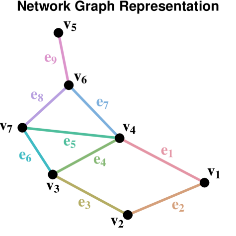
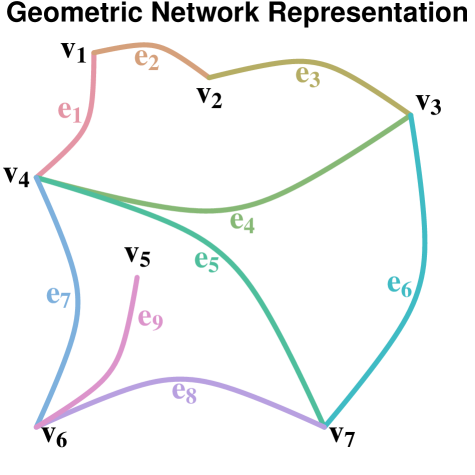
Also note that the geometric representation $\mathbold{L}$ is not necessarily unique which can be seen from the following consideration: Let $v$ be a vertex (in network graph representation) with exactly two incident edges $e_{m}=(v_{i},v)$ and $e_{n}=(v,v_{j})$, i.e. $\text{deg}(v)=2$ and $(v_{i},v_{j})\notin E$. If we remove $v$ from $V$ as well as $e_{m},e_{n}$ from $E$ but add the edge $e=(v_{i},v_{j})$ to $E$, the network graph representation of $L=(V,E)$ has changed. In the geometric representation, we can remove $\mathbold{v}$ from $\mathbold{V}$ as well as $\mathbold{e}_{m},\mathbold{e}_{n}$ from $\mathbold{E}$ and add the segment $\mathbold{e}=\mathbold{e}_{m}\cup\mathbold{e}_{n}$ to $\mathbold{E}$ which does not change $\mathbold{L}$. To exemplify the notation introduced in this section, Figure 1 shows a small network as a network graph (left panel) and as a geometric network embedded in the plane (right panel). The figure also visualizes that the function of a vertex $\mathbold{v}$ in the geometric network representation is merely being the endpoint of $\text{deg}(\mathbold{v})$ curves. Hence, in this network the vertex $\mathbold{v}_{2}$ could be removed from $\mathbold{L}$ without changing its geometric representation.

We now consider the following setting, see also McSwiggan et al. (2017). Let $\mathcal{X}$ be a stochastic point process on the geometric network $\mathbold{L}$ with continuous intensity $\varphi_{\mathcal{X}}\mathrel{\mathop{\mathchar 58\relax}}\mathbold{L}\rightarrow[0,\infty)$. The expected number of points in a set $\mathbold{K}\subset\mathbold{L}$ is then defined through

$$\int_{\mathbold}{K}\varphi_{\mathcal{X}}(\mathbold{z})\operatorname{d\!}\mathbold{z}=\sum_{m=1}^{M}\int_{\mathbold{K}\subset\mathbold{e}_{m}}\varphi_{\mathcal{X}}(\mathbold{z})\operatorname{d\!}_{\text{ }|m}\mathbold{z},$$

where $\operatorname{d\!}_{\text{ }|m}\mathbold{z}$ denotes integration with respect to the curve $\mathbold{e}_{m}$. Our aim is to estimate the intensity of the point process $\mathcal{X}$ on $\mathbold{L}$ given that we observe realizations $\mathbold{x}_{1},\dots,\mathbold{x}_{n}$ of this process. The point process $\mathcal{X}$ can equivalently be defined through a density function $f_{\mathcal{X}}\mathrel{\mathop{\mathchar 58\relax}}\mathbold{L}\rightarrow[0,\infty)$. The probability that a random point $\mathbold{X}_{i}\sim f_{\mathcal{X}}$ falls into a subset $\mathbold{K}\subset\mathbold{L}$ is then given by $\mathbb{P}(\mathbold{X}_{i}\in\mathbold{K})=\int_{\mathbold}{K}f_{\mathcal{X}}(\mathbold{z})\operatorname{d\!}\mathbold{z}$.

3 Methodology

3.1 B-Splines on a Network

First, we briefly review B-splines (compare Ruppert et al., 2003 or Fahrmeir et al., 2013). To start, assume first a simple point process $\mathcal{X}$ with intensity $\varphi_{\mathcal{X}}(z)$, where $z$ is univariate and takes values in the bounded interval $[a,b]$. The goal is to estimate $\varphi_{\mathcal{X}}(z)$ in a smooth and flexible way. To do so, we approximate the logarithmized intensity $\nu_{\mathcal{X}}=\log\varphi_{\mathcal{X}}$ through a B-spline basis representation $\nu_{\mathcal{X}}(z)=\sum_{j=1}^{J}\gamma_{j}B_{j}^{l}(z)$, where $B_{j}^{l}(\cdot)$ are B-splines of order $l\in\mathbb{N}_{0}$ and $\mathbold{\gamma}=(\gamma_{1},\dots,\gamma_{J})^{\top}$ is a vector of regression coefficients that needs to be estimated from the data. For the construction of B-splines, we use $I$ interior knots $a=\tau_{1}<\dots<\tau_{I}=b$. The $J=I+l-1$ basis functions $B_{j}^{l}(\cdot)$ are each locally supported on $l+2$ adjacent knots and can be calculated recursively from lower order basis functions (De Boor, 1972). An important property of a B-spline basis is that $\sum_{j=1}^{J}B_{j}^{l}(z)=1$ holds for $z\in[a,b]$ and any order of B-splines $l$. This property also needs to be respected in the geometric network case.

Subsequently, we restrict ourselves to linear B-spline bases for simplicity of presentation. For simplicity of notation we drop the superscript $l$ in the B-spline notation, i.e. we construct B-splines of order $l=1$ on a geometric network $\mathbold{L}$. Such a basis can be constructed straightforwardly using the one-dimensional definitions from above. On every curve $\mathbold{e}_{m}$, which has endpoints $\mathbold{v}_{i}$ and $\mathbold{v}_{j}$, we specify an equidistant sequence of $I_{m}$ knots $\mathbold{v}_{i}=\mathbold{\tau}_{m,1},\dots,\mathbold{\tau}_{m,{I_{m}}}=\mathbold{v}_{j}$ with $\mathbold{\tau}_{m,k}\in\mathbold{e}_{m}$ for $k=1,\dots,I_{m}$, where $d_{\mathbold}{L}(\mathbold{\tau}_{m,k},\mathbold{\tau}_{m,{k-1}})=\delta_{m}$. Note that a knot which is equal to a vertex $\mathbold{v}$ is contained in the knot sequence of $\text{deg}(\mathbold{v})$ segments but it is still the same knot. Unlike to the one-dimensional setup, it is in general not possible to choose the set of knots to be equidistant on the entire geometric network $\mathbold{L}$ with respect to all curve lengths $d_{m}$. However, we may choose a global knot distance $\delta$ such that it is close to an equidistant allocation of knots on the entire geometric network. Let therefore $\lceil\cdot\rceil$ denote the upwards rounded integer and $\lfloor\cdot\rfloor$ the corresponding downwards rounded integer. We then define

$$\delta_{m}=\begin{cases}d_{m}/\lfloor\frac{d_{m}}{\delta}\rfloor,\quad\frac{d_{m}}{\delta}-\lfloor\frac{d_{m}}{\delta}\rfloor<0.5\\ d_{m}/\lceil\frac{d_{m}}{\delta}\rceil,\quad\frac{d_{m}}{\delta}-\lfloor\frac{d_{m}}{\delta}\rfloor\geq 0.5\end{cases},$$ (2)

which leads to curve-specific knot distances $\delta_{m}$ which are as similar as possible for a given overall knot distance $\delta$. Generally, we will choose $\delta$ rather small such that the differences between the $\delta_{m}$ are small and can be considered as negligible. This will become more clear later, when we also introduce a penalization component in the estimation.

Having the set of knots defined as above, we can construct a linear B-spline basis $B$ on the geometric network $\mathbold{L}$. First, we use for every segment $\mathbold{e}_{m}$ with endpoints $\mathbold{v}_{i}$ and $\mathbold{v}_{j}$ the equidistant sequence of knots $\mathbold{v}_{i}=\mathbold{\tau}_{m,1},\dots,\mathbold{\tau}_{m,{I_{m}}}=\mathbold{v}_{j}$ from above to construct $J_{m}=I_{m}-2$ linear B-splines $B_{m,1},\dots,B_{m,{J_{m}}}$. These B-splines are defined accordingly to the univariate case by

$$B_{m,k}(\mathbold{z})=\frac{d_{\mathbold}{L}(\mathbold{z},\mathbold{\tau}_{m,k})}{\delta_{m}}\mathbbm{1}_{[\mathbold{\tau}_{m,k},\mathbold{\tau}_{m,k+1})}(\mathbold{z})+\frac{d_{\mathbold}{L}(\mathbold{\tau}_{m,k+2},\mathbold{z})}{\delta_{m}}\mathbbm{1}_{[\mathbold{\tau}_{m,k+1},\mathbold{\tau}_{m,k+2})}(\mathbold{z})$$ (3)

for $\mathbold{z}\in\mathbold{L},m=1,\dots,M$ and $k=1,\dots,J_{m}$. Therefore, the B-splines $B_{m,k}$ are only supported on $\mathbold{e}_{m}$ and we denote with $B_{\mathbold}{e}=\{B_{m,1},\dots,B_{m,{J_{m}}}\mid m=1,\dots,M\}$ the set of all these B-splines. We further require that $J_{m}\geq 1$ for all $m=1,\dots,M$ which is fulfilled if $\delta_{m}\leq\frac{d_{m}}{2}$ for all $m$.

Figure 2: Schematic representation of a linear B-spline basis around $\mathbold{v}_{6}$ of Figure 1. Here, $\mathbold{v}_{6}=\mathbold{\tau}_{7,1}=\mathbold{\tau}_{8,1}=\mathbold{\tau}_{9,1}$ with adjacent segments $\mathbold{e}_{7},\mathbold{e}_{8},\mathbold{e}_{9}$. The red dotted lines show the linear B-splines which are contained in $B_{\mathbold}{v}$. The peaks of all B-splines are equal to 1 as in the Euclidean setting.

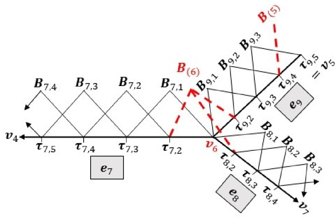
In addition to the B-splines defined by (3) we construct a single B-spline around each vertex $\mathbold{v}_{i}\in\mathbold{V}$. Therefore, we consider the $\text{deg}(\mathbold{v}_{i})$ segments which have an endpoint equal to $\mathbold{v_{i}}$ and we numerate them (without loss of generality) with $\mathbold{e}_{1},\dots,\mathbold{e}_{\text{deg}(\mathbold{v}_{i})}$. Again, without loss of generality, let $\mathbold{\tau}_{m_{1,1}}=\mathbold{v_{i}},\dots,\mathbold{\tau}_{\text{deg}(\mathbold{v}_{i}),1}=\mathbold{v_{i}}$, i.e. we order the knots such that the first knot of every segment starting in $\mathbold{v}_{i}$ equals $\mathbold{v_{i}}$, see Figure 2 as example. Then, we define the vertex specific B-spline $B_{(i)}$ for vertex $\mathbold{v}_{i}$ by

$$B_{(i)}(\mathbold{z})=\sum_{k=1}^{\text{deg}(\mathbold{v}_{i})}\left[1-\frac{d_{\mathbold}{L}(\mathbold{v}_{i},\mathbold{z})}{\delta_{k}}\right)\mathbbm{1}_{\left[\mathbold{v}_{i};\mathbold{\tau}_{k,{2}}\right)}(\mathbold{z}).$$ (4)

for $\mathbold{z}\in\mathbold{L}$ and $i=1,\dots,W$. These B-splines have support $\text{supp}(B_{(i)})=\bigcup_{k=1}^{\text{deg}(\mathbold{v}_{i})}[\mathbold{v}_{i};\mathbold{\tau}_{k,{2}})\subset\mathbold{L}$, i.e. they are supported on $\text{deg}(\mathbold{v}_{i})$ segments. Note that all summands in (4) are nonnegative and at most one of the summands is positive. This set of B-splines is denoted with $B_{\mathbold}{v}=\{B_{(1)},\dots,B_{(W)}\}$. Altogether, we specify the linear B-spline basis on $\mathbold{L}$ by $B=B_{\mathbold}{e}\cup B_{\mathbold}{v}$ with dimension $J=|B|=\sum_{m=1}^{M}J_{m}+|\mathbold{V}|$. For simplicity of presentation, we index from now on the B-spline Basis by $1,\dots,J$ and by construction, it holds that $\sum_{j=1}^{J}B_{j}(\mathbold{z})=1$ for $\mathbold{z}\in L$. In Figure 2, we depict linear B-splines around the vertex $\mathbold{v}_{6}$ with $\text{deg}(\mathbold{v}_{6})=3$ of the network that is shown Figure 1.

3.2 Intensity Estimation on a Network

Exploiting the preliminary work of this section, we can now easily adopt the density estimation approach proposed by Eilers and Marx (1996) for univariate data. On our geometric network $\mathbold{L}$, we specify a bin width $h_{m}$ on every segment $\mathbold{e}_{m}$ and then divide $\mathbold{e}_{m}$ into $N_{m}=\frac{d_{m}}{h_{m}}$ bins of the same length such that $\mathbold{L}$ is partitioned into $N=\sum_{m=1}^{M}\frac{d_{m}}{h_{m}}$ bins in total. As for the knot distances $\delta_{m}$ it is clear, that $h_{m}$ can not be same for all curve segments of $\mathbold{L}$. However, also the bin widths are chosen very small when performing intensity estimation with penalized splines. We therefore specify a small global bin width $h$ and define according to (2)

$$h_{m}=\begin{cases}d_{m}/\lfloor\frac{d_{m}}{h}\rfloor,\quad\frac{d_{m}}{h}-\lfloor\frac{d_{m}}{h}\rfloor<0.5\\ d_{m}/\lceil\frac{d_{m}}{h}\rceil,\quad\frac{d_{m}}{h}-\lfloor\frac{d_{m}}{h}\rfloor\geq 0.5\end{cases}.$$

If the the left endpoint of $\mathbold{e}_{m}$ is $\mathbold{v}$, the bins are given by the $N_{m}$ subsets $[\mathbold{b}_{m,{k-1}};\mathbold{b}_{m,k})\subset\mathbold{e}_{m}$ for $k=1,\dots,N_{m}$, where $\mathbold{b}_{m,k}\in\mathbold{e}_{m}$ satisfies $d_{\mathbold}{L}(\mathbold{v},\mathbold{b}_{m,k})=kh_{m}$ and $\mathbold{b}_{m,0}=\mathbold{v}$. Each bin is characterized by its midpoint $\mathbold{z}_{m,k}$ which satisfies $d_{\mathbold}{L}(\mathbold{b}_{m,{k-1}},\mathbold{z}_{m,k})=d_{\mathbold}{L}(\mathbold{z}_{m,k},\mathbold{b}_{m,k})$.

Assume now that data on $n$ independently observed points $\mathbold{x}_{i}$ of the point process on the geometric network have been observed, with $i=1,\ldots,n$. For identifiability reasons we assume that the observed points are not equal to the vertices of the network, i.e. each point lies on a single edge. We define with $y_{m,k}\in\mathbb{N}_{0}$ the number of observations which are contained in the $k$-th bin of the $m$-th segment, i.e.

$$y_{m,k}=\#\{\mathbold{x}_{i}\in\mathbold{L}\mid\mathbold{x}_{i}\in[\mathbold{b}_{m,{k-1}};\mathbold{b}_{m,k}),i=1,\dots,n\}$$

for $m=1,\dots,M$ and $k=1,\dots,N_{m}$. Based on our considerations for the point process $\mathcal{X}$ we assume a Poisson distribution for the counts $y_{m,k}$ such that we have

$$y_{m,k}\mid\mathbold{z}_{m,k}\overset{\text{indep.}}{\sim}\text{Poi}(\lambda_{m,k}),$$ (5)

where $\lambda_{m,k}$ is approximated through

$$\lambda_{m,k}=\varphi_{\mathcal{X}}(\mathbold{z}_{m,k})\cdot h_{m}=\exp\left(\nu_{\mathcal{X}}(\mathbold{z}_{m,k})+\log h_{m}\right).$$ (6)

We can consider $\log h_{m}$ as offset and aim to estimate $\nu_{\mathcal{X}}(\mathbold{z})$ as continuous log-intensity for $\mathbold{z}\in\mathbold{L}$ treating the pairs $(y_{m,k},\mathbold{z}_{m,k})$ as independent observations from (5). Therefore, we replace $\nu_{\mathcal{X}}(\mathbold{z})$ through the B-spline basis representation

$$\nu_{\mathcal{X}}(\mathbold{z})=\sum_{j=1}^{J}B_{j}(\mathbold{z})\gamma_{j}=\mathbold{B}(\mathbold{z})\mathbold{\gamma},$$ (7)

where $\mathbold{B}(\mathbold{z})=(B_{1}(\mathbold{z}),\dots,B_{J}(\mathbold{z}))$ is a row vector consisting of the B-spline basis evaluated at $\mathbold{z}\in\mathbold{L}$ and $\mathbold{\gamma}=(\gamma_{1},\dots,\gamma_{J})^{\top}$ is the vector of B-spline coefficients that needs to be estimated from the data $\mathbold{x}_{1},\dots,\mathbold{x}_{n}$. Imposing a penalty on the resulting Poisson likelihood leads to the penalized log-likelihood (constant terms are ignored)

$$\ell_{\mathcal{P}}(\mathbold{\gamma};\rho)=\sum_{m=1}^{M}\sum_{k=1}^{N_{m}}\left[y_{m,k}\mathbold{B}(\mathbold{z}_{m,k})\mathbold{\gamma}-\exp\left(\mathbold{B}(\mathbold{z}_{m,k})\mathbold{\gamma}+\log h_{m}\right)\right]-\rho\mathcal{P}_{r}(\mathbold{\gamma}),$$ (8)

where $\mathcal{P}_{r}(\mathbold{\gamma})$ is a penalty which is defined in the next section and $\rho$ is the smoothing parameter. It is also shown later how this smoothing parameter can be estimated.

If we replace $\mathbold{\gamma}$ in (7) with the maximum-likelihood estimate $\widehat{\mathbold{\gamma}}=\text{argmax}_{\mathbold}{\gamma}\ell_{\mathcal{P}}(\mathbold{\gamma};\rho)$, then $\widehat{\nu}_{\mathcal{X}}(\mathbold{z})=\mathbold{B}(\mathbold{z})\widehat{\mathbold{\gamma}}$ is an estimate of the log-intensity and thus $\widehat{\varphi}_{\mathcal{X}}(\mathbold{z})=\exp\left(\widehat{\nu}_{\mathcal{X}}(\mathbold{z})\right)$ is an estimate of the intensity of the point process $\mathcal{X}$ for $\mathbold{z}\in\mathbold{L}$. Also note that for a given $n$ an estimate of the density of $\mathcal{X}$ is given by $\widehat{f}_{\mathcal{X}}(\mathbold{z})=\widehat{\varphi}_{\mathcal{X}}(\mathbold{z})/n.$

3.3 Penalties on a Network

In order to control smoothness of the intensity estimate and to overcome singularity issues, the penalty $\mathcal{P}_{r}(\mathbold{\gamma})$ multiplied with the smoothing parameter $\rho$ is subtracted from the maximum likelihood criterion, which leads to the penalized log-likelihood (8). Eilers and Marx (1996) proposed to impose a penalty on the vector of coefficients $\mathbold{\gamma}$ that is proportional to the $r$-th order differences of adjacent spline coefficients. The penalty is given by $\sum_{j=r+1}^{J}(\Delta^{r}\gamma_{j})^{2}$ and for $r=1$ we have $\Delta^{1}\gamma_{j}=\gamma_{j}-\gamma_{j-1}$. Higher order penalty terms can be calculated recursively using $\Delta^{r}(\gamma_{j})=\Delta^{1}\Delta^{r-1}\gamma_{j}$ starting with the first order differences $\Delta^{1}\gamma_{j}$. It is straightforward to extend this idea to penalties on a network. Let $i,j=1,\dots,J$ where $J$ is the dimension of the B-spline basis on the geometric network. According to the one-dimensional case, we are interested in the set of pairwise adjacent B-splines or their coefficients, respectively. Hence, we can view the B-splines on the geometric network $\mathbold{L}$ itself as a network graph $L_{B}$ which is defined through a $J\times J$ adjacency matrix $\mathbold{A}$. From the definition of the linear B-splines, it follows that $\mathbold{A}(i,j)=1$, if $\text{supp}(B_{i})\cap\text{supp}(B_{j})\neq\emptyset$ and else $\mathbold{A}(i,j)=0$. In order to define penalties of arbitrary order, we need the $J\times J$ shortest path matrix $\mathbold{S}_{\mathbold}{A}$ where $\mathbold{S}_{\mathbold}{A}(i,j)=s$, if the B-Splines $B_{i}$ and $B_{j}$ have minimum distance $s$ in $L_{B}$. This all-pairs shortest path problem can be solved with complexity $\mathcal{O}(J|\mathcal{A}|)$ where $|\mathbold{A}|$ is the number of non-zero entries in $\mathbold{A}$ (Chan, 2012). For illustration, consider again Figure 2. Here, $B_{7,1}$ is adjacent to $B_{7,2}$ as well as $B_{(6)}$ and the shortest path from $B_{7,2}$ to $B_{8,1}$ via $B_{7,1}$ and $B_{(6)}$ has length $3$ in $L_{B}$.

Now, let $\mathcal{D}_{1}=\{(i,j)\mid\mathbold{S}_{\mathbold}{A}(i,j)=1,1\leq i<j\leq J\}$. According to Eilers and Marx (1996) we penalize neighboring coefficients. A first order penalty is then defined by

$$\mathcal{P}_{1}(\mathbold{\gamma})=\sum_{\mathcal{D}_{1}}(\gamma_{i}-\gamma_{j})^{2}=(\mathbold{D}_{1}\mathbold{\gamma})^{\top}(\mathbold{D}_{1}\mathbold{\gamma})=\mathbold{\gamma}^{\top}\mathbold{K}_{1}\mathbold{\gamma},$$ (9)

where $\mathbold{D}_{1}\in\mathbb{Z}^{|\mathcal{D}_{1}|\times J}$ and $\mathbold{K}_{1}=\mathbold{D}_{1}^{\top}\mathbold{D}_{1}\in\mathbb{Z}^{J\times J}$ define the difference matrix and the resulting quadratic form according to the pairwise differences in (9). Further, let

$$\mathcal{D}_{2}=\{(i,k,j)\mid\mathbold{S}_{\mathbold}{A}(i,j)=2,\mathbold{S}_{\mathbold}{A}(i,k)=\mathbold{S}_{\mathbold}{A}(k,j)=1,1\leq i<j\leq J\}.$$

Therewith, a second order penalty can be defined by

$$\mathcal{P}_{2}(\mathbold{\gamma})=\ \sum_{\mathcal{D}_{2}}((\gamma_{i}-\gamma_{k})-(\gamma_{k}-\gamma_{j}))^{2}=\ \sum_{\mathcal{D}_{2}}(\gamma_{i}-2\gamma_{k}+\gamma_{j})^{2}=(\mathbold{D}_{2}\mathbold{\gamma})^{\top}(\mathbold{D}_{2}\mathbold{\gamma})=\mathbold{\gamma}^{\top}\mathbold{K}_{2}\mathbold{\gamma},$$ (10)

where $\mathbold{D}_{2}\in\mathbb{Z}^{|\mathcal{D}_{2}|\times J}$ and again, $\mathbold{K}_{2}=\mathbold{D}_{2}^{\top}\mathbold{D}_{2}\in\mathbb{Z}^{J\times J}$ results as matrix version from the sum in (10). For illustration, we revisit the B-splines which we depict in Figure 2, but, restricted to the B-splines $B_{1}=B_{7,2},B_{2}=B_{7,1},B_{3}=B_{(6)},B_{4}=B_{8,1}$ and $B_{5}=B_{9,1}$. Thus, for $\mathbold{\gamma}=(\gamma_{1},\dots,\gamma_{5})$ the first- and second order penalties $\mathcal{P}_{1}(\mathbold{\gamma})$ and $\mathcal{P}_{2}(\mathbold{\gamma})$ are defined by the difference matrices

$$\mathbold{D}_{1}=\begin{pmatrix}1&-1&0&0&0\\ 0&1&-1&0&0\\ 0&0&1&-1&0\\ 0&0&1&0&-1\end{pmatrix}\quad\text{and}\quad\mathbold{D}_{2}=\begin{pmatrix}1&-2&1&0&0\\ 0&1&-2&1&0\\ 0&1&-2&0&1\\ 0&0&-2&1&1\end{pmatrix},$$

respectively. Exploiting the shortest path matrix $\mathbold{S}_{\mathbold}{A}$ we can define penalties of any order $r$, but usually first and second order differences are used when applying penalized splines.

3.4 Estimation of the Smoothing Parameter

For the estimation of the smoothing parameter $\rho$, we apply the generalized Fellner-Schall method (Wood and Fasiolo, 2017) which is an iterative procedure to estimate the smoothing parameter in generalized additive models (Wood, 2017). The idea behind the Fellner-Schall method is to apply a mixed model approach and to compute the log Laplace approximate marginal likelihood of the model and its derivative with respect to the smoothing parameter $\rho$. In each iteration step we estimate the model parameters $\widehat{\mathbold{\gamma}}_{\rho}$ by maximizing the penalized log-likelihood (8) while taking $\rho$ from the previous cycle. Then, the update $\rho_{\text{new}}$ is calculated through

$$\rho_{\text{new}}=\rho\frac{\text{tr}((\rho\mathbold{K}_{r})^{-}\mathbold{K}_{r})-\text{tr}((\mathbold{B}^{\top}\mathbold{W}(\widehat{\mathbold{\gamma}}_{\rho})\mathbold{B}+\rho\mathbold{K}_{r})^{-1}\mathbold{K}_{r})}{\widehat{\mathbold{\gamma}}_{\rho}^{\top}\mathbold{K}_{r}\widehat{\mathbold{\gamma}}_{\rho}}$$ (11)

where $\text{tr}(\cdot)$ denotes the trace operator for diagonal matrices and $(\rho\mathbold{K}_{r})^{-}$ denotes a generalized inverse of $\rho\mathbold{K}_{r}$. The design matrix $\mathbold{B}\in\mathbb{R}^{N\times J}$ of the Poisson model is build by storing the row vectors $\mathbold{B}(\mathbold{z}_{m,k})$, which are defined accordingly to (7) for $m=1,\dots,M$ and $k=1,\dots,N_{m}$, as a matrix. Furthermore, $\mathbold{W}(\widehat{\mathbold{\gamma}}_{\rho})=\text{diag}(\widehat{\lambda}_{1,1},\dots,\widehat{\lambda}_{1,N_{1}},\dots,\widehat{\lambda}_{M,1},\dots,\widehat{\lambda}_{M,N_{M}})$ is a weight matrix, where $\widehat{\lambda}_{m,k}=\exp\left(\widehat{\gamma}_{\mathcal{X}}(\mathbold{z}_{m,k})+\log h_{m}\right)$ is defined through (6). The matrix $\mathbold{B}^{\top}\mathbold{W}(\widehat{\mathbold{\gamma}}_{\rho})\mathbold{B}+\rho\mathbold{K}_{r}$ is the expected Hessian of our model and is therefore positive definite, which guarantees that $\rho_{\text{new}}>0$ (Wood and Fasiolo, 2017). The iterative procedure stops, if $\rho_{\text{new}}$ in (11) differs only slightly from $\rho$.

4 Simulation Study

Figure 3: Simple network with $n=5,20,100,1000$ uniformly distributed random points (left panels); Intensity estimates based on penalized splines (middle panels) and kernel estimation (right panels).

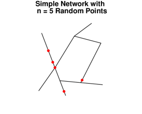
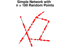
In this section we exploit simulated data in order to explore the performance of penalized spline intensity estimation on geometric networks. The general setting of this study is that we consider the rather small network simplenet from the spatstat package (Baddeley et al., 2015) with $|\mathbold{E}|=|\mathbold{V}|=10$ and total length $|\mathbold{L}|=2.905$. On this network we specify an intensity function $\varphi_{\mathcal{X}_{n}}$, where $\int_{\mathbold}{L}\varphi_{\mathcal{X}_{n}}(\mathbold{z})\operatorname{d\!}\mathbold{z}=n$. Therefore, we independently simulate $n$ random points according to $\varphi_{\mathcal{X}_{n}}$ and estimate the intensity of the simulated point process with penalized spline smoothing. This is opposed to a kernel based intensity estimate with automatic bandwidth selection as implemented in the spatstat package. Our routine is also implemented in R and heavily exploits the geometric network representation of the spatstat package. Here, a geometric network is embedded in the plane and consists merely of straight line segments, but we can align several line segments to a piecewise linear curve.

4.1 Uniform Intensity – Graphical Comparison with Kernel Based Estimation

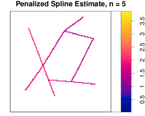
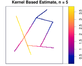
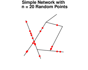
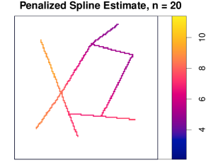
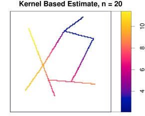
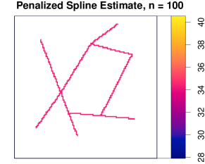
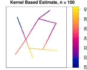
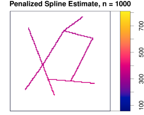
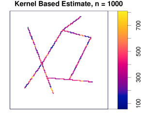
To begin with, we specify a uniform intensity on $\mathbold{L}$, i.e. $\varphi_{\mathcal{X}_{n}}(\mathbold{z})=n/|\mathbold{L}|$ for all $\mathbold{z}\in\mathbold{L}$. We independently simulate random samples $\{\mathbold{x}_{1},\dots,\mathbold{x}_{n}\}$ for $n=5,20,100,1000$ according to $\varphi_{\mathcal{X}_{n}}$. The four exemplary simulated point processes on $\mathbold{L}$ are shown in the left panels of Figure 3. We estimate the intensity of these processes exploiting both, the penalized spline and the kernel based approach. For the former method, we use $\delta=0.05,h=0.01$ with a first-order penalty.

When estimating the smoothing parameter with $n=100$ we get $\widehat{\rho}\rightarrow\infty$ such that the penalty on the log-likelihood of the model affects $\widehat{\gamma}_{1}\approx\dots\approx\widehat{\gamma}_{P}$. Therefore, when using the penalized spline method we estimate nearly a constant intensity, i.e. $\widehat{\varphi}_{\mathcal{X}_{100}}(\mathbold{z})\approx 100/{|\mathbold{L}|}=34.432$ for all $\mathbold{z}\in\mathbold{L}$, which can be observed in the middle panel of the third row in Figure 3. The optimal bandwidth $\widehat{\kappa}$ for $n=100$ when using the kernel method is $\widehat{\kappa}=0.276$. In contrast to our method, the intensity calculated therewith yields values for $\widehat{\varphi}_{\mathcal{X}_{100}}(\mathbold{z})$ within the interval $[28,40]$, see the right panel of the third row in Figure 3. This originates from the locality of the kernel smoother.

A more extreme discrepancy between the two estimation methods is observable for $n=1000$, see the bottom row of Figure 3. Again, our method estimates a nearly constant intensity whereas the kernel method yields a very rough estimate. Here, the bandwidth selection algorithm estimates an optimal bandwidth of $\widehat{\kappa}=0.0063$, which is very small compared to the length of the single line segments. Furthermore, the top two rows of Figure 3 show that even with a small sample size, we are still able to roughly estimate a constant intensity with our method and again, the kernel based method leads to a very high variation in the intensity estimate along the geometric network.

Figure 4: Mean and standard deviation of penalized spline based and kernel based ISE for $n=5,10,20,50,100,200,500,1000$ on a log-log-scale, where $\varphi_{\mathbold{X}_{n}}$ is defined according to a uniform intensity on $\mathbold{L}$.

Uniform Intensity	$h=0.1$	$h=0.05$	$h=0.01$	$h=0.005$
$\delta=0.1$	1.65 (4.19)	2.24 (5.14)	1.91 (4.72)	2.24 (6.08)
$\delta=0.05$	–	2.08 (5.62)	2.40 (5.71)	2.15 (5.03)
$\delta=0.01$	–	–	1.97 (5.29)	2.18 (5.57)

Table 1: Mean (standard deviation) of ISE if $\varphi_{\mathcal{X}_{n}}$ follows a uniform intensity on $\mathbold{L}$ with $n=100$ as well as different choices of $\delta$ and $h$. All values in this table are multiplied by factor 1,000.

4.2 Uniform Intensity – Integrated Squared Error

Figure 5: Top panel: Plot of $\varphi_{\mathcal{X}_{n}}$ according to (12) with $n=1$; Mean (bottom left panel) and standard deviation (bottom right panel) of penalized spline based and kernel based ISE for $n=5,10,20,50,100,200,500,1000$ with true intensity (12) on a log-log-scale.

Non-Uniform Intensity	$h=0.1$	$h=0.05$	$h=0.01$	$h=0.005$
$\delta=0.1$	7.67 (5.33)	7.89 (5.46)	7.73 (5.25)	7.92 (4.93)
$\delta=0.05$	–	7.51 (4.36)	7.62 (4.67)	7.85 (5,40)
$\delta=0.01$	–	–	6.81 (4.18)	7.78 (5.16)

Table 2: Mean (standard deviation) of ISE with $\varphi_{\mathcal{X}_{n}}$ as in (12) for $n=100$ as well as different choices of $\delta$ and $h$. All values in this table are multiplied by factor 1,000.

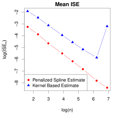
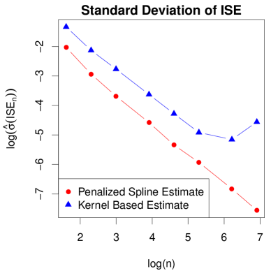
We extend the above setting with multiple simulations per sample size and set $\delta=0.05,h=0.01,r=1$. We also use several values of $n$ to assess consistency. To do so we simulate $S=1000$ networks for $n=5,10,20,50,100,200,500,1000$ and quantify the estimation error of the $s$-th simulation through

$$\text{ISE}_{n}(s)=\frac{1}{n^{2}}\int_{\mathbold}{L}\left(\varphi_{{\cal X}_{n}}(\mathbold{z})-\widehat{\varphi}_{{\cal X}_{n}}(\mathbold{z};s)\right)^{2}\operatorname{d\!}\mathbold{z},$$

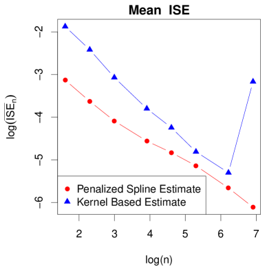
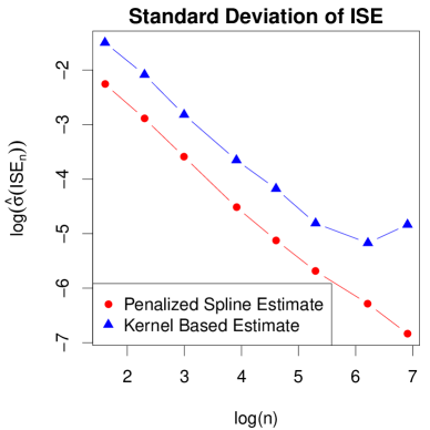
where $\widehat{\varphi}_{\mathcal{X}_{n}}(\cdot;s)$ denotes the estimate of $\varphi_{\mathcal{X}_{n}}$ based on the $s$-th sample. That is, we quantify the estimation error through the integrated squared error (ISE) between the true density $f_{\mathcal{X}}(\mathbold{z})=\varphi_{\mathcal{X}_{n}}(\mathbold{z})/n=1/|\mathbold{L}|$ and the estimated density $\widehat{f}_{\mathcal{X}}(\mathbold{z})=\widehat{\varphi}_{\mathcal{X}_{n}}(\mathbold{z})/n$. The resulting means $\overline{\text{ISE}_{n}}$ over all $S=1000$ simulations and the corresponding standard deviations $\widehat{\sigma}(\text{ISE}_{n})$ for penalized spline and kernel based estimation are shown in Figure 4. We can clearly see that the penalized spline approach performs distinctly superior to the kernel based approach in terms of ISE. Even more, for $n=1,000$ sample points we see that the latter method does perform poorly. Regarding the bottom right panel of Figure 3, we suppose that this results from very small bandwidths that are estimated from the data. For the penalized spline approach we see that the mean and the standard deviation of $\text{ISE}_{n}$ decrease nearly linearly on a log-log-scale with the number of random points $n$.

We also explore the effect of the bin width $h$ and the dimension $J$ of the B-spline basis, which is determined by the knot distance $\delta$. We only consider cases where $h\leq\delta$ and restrict this analysis on the sample size $n=100$. The results in Table 1 show that the mean ISE over $S=1000$ simulations does not vary significantly with different choices of $\delta$ and $h$. This is in line with the motivating arguments in Eilers and Marx (1996) and corresponds to the general results for penalized spline smoothing as derived in Kauermann and Opsomer (2011).

4.3 Non-Uniform Intensity – Integrated Squared Error

In order to investigate the performance of penalized spline based intensity estimation also for non-uniform intensities, we consider now the intensity function

$$\varphi_{\mathcal{X}_{n}}(\mathbold{z})=\sqrt{y}\exp(-xy)\cdot\frac{n}{C}$$ (12)

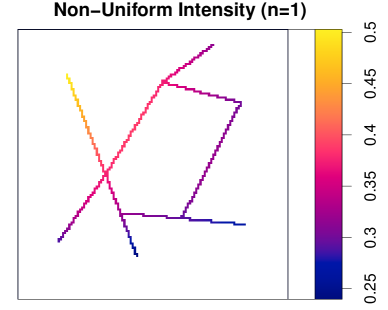
on the above network, which is shown in the top panel of Figure 5. Here, $\mathbold{z}=(x,y)^{\top}$ is the plane-coordinate representation of a point $\mathbold{z}\in\mathbold{L}$ with $0\leq x,y\leq 1$ and $C\approx 1.558$ is the normalization constant such that $\int_{\mathbold}{L}\varphi_{\mathcal{X}_{n}}\operatorname{d\!}\mathbold{z}=n$. In the bottom row of Figure 5 we oppose the means (bottom left panel) and standard deviations (bottom right panel) of $S=1000$ ISE samples for both, penalized spline and kernel based intensity estimation using the same parameter setting as in the uniform case from above. We can see that also here the penalized spline method is distinctly superior to the kernel based approach in terms of ISE. Furthermore, the decrease of the mean ISE is still linear on a log-log-scale but the relationship is not as strong as in the uniform case. Finally, we repeat the simulation study with $\varphi_{\mathcal{X}_{n}}$ as in (12), $S=1000$ simulations, $n=100,r=1$ and several choices for $\delta$ and $h$. Again, there is no recognizable effect of the overall knot distance $\delta$ and the overall bin width $h$ on the mean ISE, which can be observed from Table 2.

5 Application

5.1 Crimes in a District of Chicago

As first application with real data we consider the Chicago crimes network which is also implemented in the spatstat package and elaborated in detail in Baddeley et al. (2015). The top panel of Figure 6 shows the location of 116 crimes recorded over a two-week period in 2002 in a district of Chicago (neglecting the kind of crime). This network consists of $|\mathbold{E}|=503$ line segments and $|\mathbold{V}|=338$ vertices with a total length of $|\mathbold{L}|=31,150.21$ feet. Even though the sample size $n=116$ is small for this rather large network, it seems very unlikely that the point pattern, which is displayed in the top panel of Figure 6, originates from a uniform distribution on $\mathbold{L}$. Most of the crimes seem to occur in the northeastern and northwestern parts of the map extract.

Figure 6: Chicago crime network (top panel); Penalized spline intensity estimate (bottom left panel) and kernel based intensity estimate (bottom right panel).

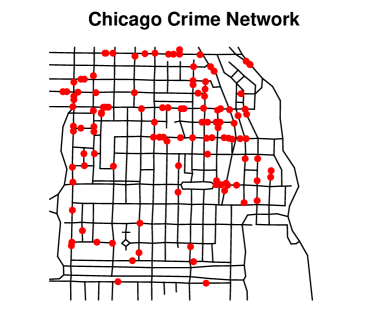
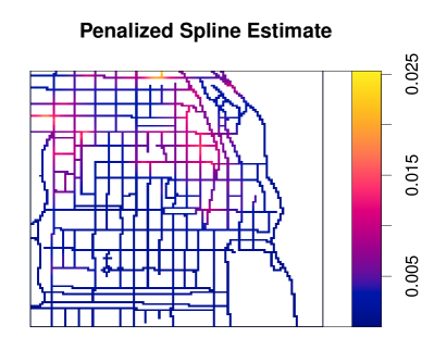
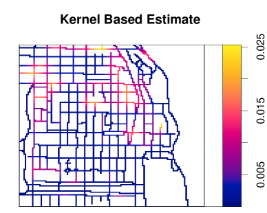
When estimating the intensity with the approach of Section 3, we use $\delta=5,h=1$ and a first-order penalty. The lower panels of Figure 6 show the estimates resulting from the data using a penalized spline based approach (left panel) or a kernel based estimation (right panel). We find that the high-intensity regions are similarly located for both methods. However, the peaks of the kernel intensity estimate are more explicit and the intensity fitted with the penalized spline approach is more smooth. When considering the few events in the southern area of the map extract, a peak occurs in the kernel intensity estimate which is not visible in the spline approach. Taking the performance of the kernel density estimates as shown in the simulated data above into account, it seems plausible to consider crime events to be uniformly distributed over the southern part of the network, that is, the peaky behavior of the kernel methods seems misleading.

5.2 On-Street Parking in Melbourne

Between August 2011 and May 2012, the City of Melbourne, Australia, installed in-ground sensors underneath around $4,600$ out of more than $20,000$ on-street parking lots in the Central Business District (CBD) of Melbourne. These sensors are able to record the arrival time and the departing time of a car to the second. Our goal is to detect regions in the CBD where the occupation of on-street parking lots fluctuates most. Therefore, we define an event to be the clearing of an on-street parking lot and the point process that we observe now has a spatial as well as a temporal structure. We here concentrate on the spatial structure only.

Figure 7: The western CBD of Melbourne, Australia: Parking bays with installed in-ground sensors within the specified geometric network (left panel); Penalized spline estimate of the intensity of parking lots on this network (right panel).

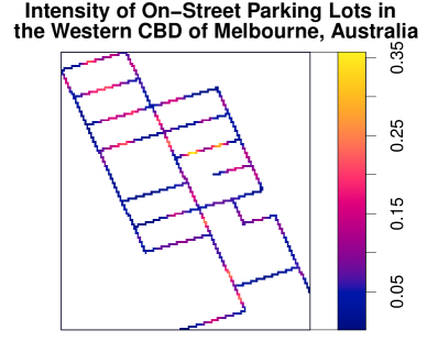
For reasons of simplicity, we only consider a subset of 518 on-street parking lots with installed in-ground sensors, which are all located in the western CBD of Melbourne. To estimate the fluctuation rate, we first need to specify a geometric network where the point process is living on. This network is constructed by excluding edges (i.e. streets in this area) without installed parking lots, since by definition we can not observe parking events on these streets. In Figure 7 we show the location of the considered on-street parking lots on the corresponding geometric network, which consists of $|\mathbold{E}|=41$ line segments, $|\mathbold{V}|=32$ vertices and has a length of nearly 7 kilometers. In order to estimate the fluctuation rate, we also need to estimate the intensity $\varphi_{\mathcal{Z}}$ of parking lots along the geometric network $\mathbold{L}$. The fitted intensity $\widehat{\varphi}_{\mathcal{Z}}$ of allocated parking lots using the penalized spline based approach is depicted in the right panel of Figure 7. Note that this estimate is not based on data on cleared parking lots but on the existence of the lots itself. In other words, this estimate may serve as baseline subsequently, since in areas with more allocated parking lots there is per se a higher chance of finding a cleared lot.

We now look at cleared parking lots and consider data in the hourly intervals between 8 and 9 am in the morning as well as 5 and 6 pm in the evening. We take data on working days over the year 2017 and consider these data as results of the clearing point process $\mathcal{Y}$, whose intensity $\varphi_{\mathcal{Y}}$ is again estimated using penalized spline smoothing. Overall we are interested in the ratio $\varphi_{\mathcal{X}}=\varphi_{\mathcal{Y}}/\varphi_{\mathcal{Z}}$, which expresses the expected fluctuation rate of parking lots along the network. However, we are only interested in the fluctuation rate where we expect a reasonable number of parking lots. Therefore, we show in Figure 8 the estimated fluctuation rates $\widehat{\varphi}_{\mathcal{X}}(\mathbold{z})$ only at locations $\mathbold{z}\in\mathbold{L}$ where $\widehat{\varphi}_{\mathcal{Z}}(\mathbold{z})\geq 0.1$, i.e. where we expect at least one on-street parking lot per 10 meters. Furthermore, the rates are normalized such that $\widehat{\varphi}_{\mathcal{X}}(\mathbold{z})$ can be interpreted as the expected hourly fluctuation rate of a parking lot, which is located at $\mathbold{z}\in\mathbold{L}$.

Figure 8: Fluctuation rate (per hour) of on-street parking lots in the western CBD of Melbourne where we expect at least one parking lot per 10 meters: Between 8 and 9 am (left panel); Between 5 and 6 pm (right panel).

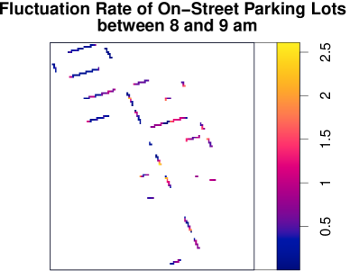
When we examine Figure 8, we can see that the high intensity regions distinguish between the hour in the morning (left panel) and the hour in the evening (right panel). In the former case, the highest fluctuation rate with around 3 clearances per parking lot and hour can be observed in parts of the central north/south road (King Street) of this map extract. In the latter case, we see a much lower fluctuation rate in King Street but a much higher fluctuation rate in the northwestern part of the map extract, especially in Lonsdale Street between King Street and William Street. Here, we have the highest intensity of parking lots $\varphi_{\mathcal{Z}}$ but also numerous clearing events that we observe between 5 and 6 pm.

6 Discussion and further Work

In this article we developed a new method for the estimation of the intensity (or density) of a stochastic process living on a geometric network. We exploited and extended penalized spline estimation to work on a subset of connected curves which we denoted as geometric networks. Note that by our definition, an interval $[a,b]$ is a special case of a geometric network $\mathbold{L}$ with $|\mathbold{E}|=1$ and $|\mathbold{V}|=2$. Our results show that penalized spline based smoothing on geometric networks benefits over the current state of the art estimation based on kernel smoothing.

As seen in the simulation study and the application examples, the penalization also compensates for non-equidistant knots and bin widths on different segments of $\mathbold{L}$. However, these differences can be made as small as desired by reducing $\delta$ and $h$. In the end, this leads to a trade-off between accuracy and computational effort. In an Euclidean space, the penalties that are used for estimation with B-splines are often based on derivatives of the smoother. However, in a geometric network the question arises how one could define differentiability of a function $f$ at vertices $\mathbold{v}$ with $\text{deg}(\mathbold{v})>2$. Apparently, adapting the penalization technique of Eilers and Marx (1996) circumvents this question and proves to be the right choice for our setting.

We envisage many more generalizations and extensions of our method. First the linear penalized spline approach could be extended to work with higher order penalized splines, in particular with quadratic or cubic penalized splines. Therewith, the estimated intensities could become even more smoother along the network. However, B-splines of order 2 or higher in Euclidean spaces are differentiable. Therefore, as stated above it would be much more complicated to construct network based B-splines of order 2 or higher around vertices $\mathbold{v}$ with $\text{deg}(\mathbold{v})>2$.

Furthermore, if we drop the assumption that the network graph $L$ should not be directed, we need the geometric representation $\mathbold{L}$ to be possibly directed as well. This means that a curve $\mathbold{e}_{m}$ additionally is equipped with a direction if $e_{m}=(v_{i},v_{j})$ is a directed edge from $v_{i}$ to $v_{j}$ but there is no edge from $v_{j}$ to $v_{i}$. In this case, the distance measure $d_{\mathbold}{L}$ from above does not define a metric any more since then, $d_{\mathbold}{L}(\mathbold{z_{1}},\mathbold{z}_{2})=d_{\mathbold}{L}(\mathbold{z_{2}},\mathbold{z}_{1})$ for $\mathbold{z_{1}},\mathbold{z_{2}}\in\mathbold{L}$ does not hold in general.

Apart from estimating intensities, our construction of linear B-splines on a geometric network also allows to include a network specific covariate in a regression model. For example, the time until a parking lot is reoccupied after a car has left can be explained by covariates such as time of the day, weather conditions, etc. But also the location of the parking lot in the street network might be an explanatory variable which can be smoothly modeled with our penalized spline approach.

And finally, the time aspect can be incorporated as well, leading to simultaneous smoothing over the geometric network and time. We consider these aspects beyond the scope of the current paper but see high potential for future research. For example, it would be interesting how the fluctuation rates in the Melbourne parking network vary during the course of the year.

References

- Ang et al. (2012) Ang, Q. W., A. Baddeley, and G. Nair (2012). Geometrically corrected second order analysis of events on a linear network, with applications to ecology and criminology. Scandinavian Journal of Statistics 39(4), 591–617.
- Baddeley et al. (2015) Baddeley, A., E. Rubak, and R. Turner (2015). Spatial point patterns: methodology and applications with R. Chapman and Hall/CRC.
- Bassett and Sharpnack (2018) Bassett, R. and J. Sharpnack (2018). Fused density estimation: Theory and methods. arXiv preprint arXiv:1805.03288.
- Beer (2013) Beer, G. (2013). The structure of extended real-valued metric spaces. Set-Valued and Variational Analysis 21(4), 591–602.
- Borruso (2008) Borruso, G. (2008). Network density estimation: a gis approach for analysing point patterns in a network space. Transactions in GIS 12(3), 377–402.
- Chan (2012) Chan, T. M. (2012). All-pairs shortest paths for unweighted undirected graphs in o (mn) time. ACM Transactions on Algorithms (TALG) 8(4), 1–17.
- Currie et al. (2006) Currie, I. D., M. Durban, and P. H. Eilers (2006). Generalized linear array models with applications to multidimensional smoothing. Journal of the Royal Statistical Society: Series B (Statistical Methodology) 68(2), 259–280.
- De Boor (1972) De Boor, C. (1972). On calculating with B-splines. Journal of Approximation theory 6(1), 50–62.
- Diggle (1985) Diggle, P. (1985). A kernel method for smoothing point process data. Journal of the Royal Statistical Society: Series C (Applied Statistics) 34(2), 138–147.
- Eilers and Marx (1996) Eilers, P. H. and B. D. Marx (1996). Flexible smoothing with B-splines and penalties. Statistical Science 11, 89–102.
- Eilers et al. (2015) Eilers, P. H., B. D. Marx, and M. Durbán (2015). Twenty years of P-splines. SORT: statistics and operations research transactions 39(2), 0149–186.
- Fahrmeir et al. (2013) Fahrmeir, L., T. Kneib, S. Lang, and B. Marx (2013). Regression. Springer.
- Goldenberg et al. (2010) Goldenberg, A., A. X. Zheng, S. E. Fienberg, E. M. Airoldi, et al. (2010). A survey of statistical network models. Foundations and Trends® in Machine Learning 2(2), 129–233.
- Heuser (2006) Heuser, H. (2006). Lehrbuch der Analysis 1, 2. Teubner, Stuttgart.
- Kauermann and Opsomer (2011) Kauermann, G. and J. D. Opsomer (2011). Data-driven selection of the spline dimension in penalized spline regression. Biometrika 98(1), 225–230.
- Kolaczyk and Csárdi (2014) Kolaczyk, E. D. and G. Csárdi (2014). Statistical analysis of network data with R, Volume 65. Springer.
- McSwiggan et al. (2017) McSwiggan, G., A. Baddeley, and G. Nair (2017). Kernel density estimation on a linear network. Scandinavian Journal of Statistics 44(2), 324–345.
- Moradi et al. (2018) Moradi, M. M., F. J. Rodríguez-Cortés, and J. Mateu (2018). On kernel-based intensity estimation of spatial point patterns on linear networks. Journal of Computational and Graphical Statistics 27(2), 302–311.
- O’Donnell et al. (2014) O’Donnell, D., A. Rushworth, A. W. Bowman, E. Marian Scott, and M. Hallard (2014). Flexible regression models over river networks. Journal of the Royal Statistical Society: Series C (Applied Statistics) 63(1), 47–63.
- Okabe et al. (2009) Okabe, A., T. Satoh, and K. Sugihara (2009). A kernel density estimation method for networks, its computational method and a gis-based tool. International Journal of Geographical Information Science 23(1), 7–32.
- Okabe and Yamada (2001) Okabe, A. and I. Yamada (2001). The K-function method on a network and its computational implementation. Geographical Analysis 33(3), 271–290.
- Okabe et al. (1995) Okabe, A., H. Yomono, and M. Kitamura (1995). Statistical analysis of the distribution of points on a network. Geographical Analysis 27(2), 152–175.
- Rasmussen and Christensen (2018) Rasmussen, J. G. and H. S. Christensen (2018). Point processes on directed linear network. arXiv preprint arXiv:1812.09071.
- Ruppert et al. (2003) Ruppert, D., M. P. Wand, and R. J. Carroll (2003). Semiparametric regression. Number 12. Cambridge university press.
- Ruppert et al. (2009) Ruppert, D., M. P. Wand, and R. J. Carroll (2009). Semiparametric regression during 2003–2007. Electronic journal of statistics 3, 1193.
- Rushworth et al. (2015) Rushworth, A., E. Peterson, J. Ver Hoef, and A. Bowman (2015). Validation and comparison of geostatistical and spline models for spatial stream networks. Environmetrics 26(5), 327–338.
- Schellhase and Kauermann (2012) Schellhase, C. and G. Kauermann (2012). Density estimation and comparison with a penalized mixture approach. Computational Statistics 27(4), 757–777.
- Snijders (1996) Snijders, T. A. (1996). Stochastic actor-oriented models for network change. Journal of mathematical sociology 21(1-2), 149–172.
- Spooner et al. (2004) Spooner, P. G., I. D. Lunt, A. Okabe, and S. Shiode (2004). Spatial analysis of roadside acacia populations on a road network using the network k-function. Landscape ecology 19(5), 491–499.
- Wood (2017) Wood, S. N. (2017). Generalized additive models: an introduction with R. Chapman and Hall/CRC.
- Wood and Fasiolo (2017) Wood, S. N. and M. Fasiolo (2017). A generalized Fellner-Schall method for smoothing parameter optimization with application to tweedie location, scale and shape models. Biometrics 73(4), 1071–1081.
- Xie and Yan (2008) Xie, Z. and J. Yan (2008). Kernel density estimation of traffic accidents in a network space. Computers, environment and urban systems 32(5), 396–406.