Computational study of the dynamics of an asymmetric wedge billiard

Abstract

We introduce the asymmetric wedge billiard as a generalization of the wedge billiard first introduced and studied by Lehtihet and Miller in 1986. This is a billiard system in which the billiard ball moves under the influence of a constant gravitational field, colliding elastically with two wedge walls with the collisions obeying the reflection law. Collision maps are given from which derivatives and area-preservation (or lack thereof) were determined. Expressions for the fixed points of the collision maps were also calculated and discussed. Long-term dynamics were determined computationally from which we observed integrable, quasi-periodic and chaotic behaviour which were all dependent on the wedge angles.

1 Introduction

A dynamical billiard system consists of a particle represented as a geometric point moving freely within a bounded region in the plane, its collisions with the boundary of the region are elastic and obey the reflection law.

G.D. Birkhoff [6] introduced dynamical billiards as a means to prove Poincaré’s last geometric conjecture. Others [4, 22, 28] continued his work on convex billiards with some open questions remaining to this day. The seminal work by Y.G. Sinai [32] introduced a new class of billiards, called dispersing billiards, as an application to modelling Lorentz gas and was the first to show that these billiard systems are chaotic. Another class of billiards, i.e., polygonal billiards, arose naturally from the study of another mechanical system, that of two point particles moving on a straight line between two walls. This shows the utility of dynamical billiards, as Birkhoff himself stated that most Hamiltonian systems with two degrees of freedom could be studied by the appropriate transform to a dynamical billiard. Standard billiard dynamics are quite rich and numerous open problems remain.

Research has also been done on modifications of classical billiard systems. It would be natural to consider the particle moving in the quantum realm [7, 37, 39] or moving relativistically [11, 12, 13]. Other billiard systems consider modifications to the region of motion itself, for example, a hole or multiple holes within the region—these are the so-called “open billiards”; billiard systems where the boundary changes in time [18, 19, 21, 24, 25, 26]; and billiard systems where the billiard moves under the influence of a constant force field, either magnetic [3, 10, 14, 30, 38] or gravitational [9, 20, 23].

The wedge billiard (illustrated in Figure 1) is a billiard system where the particle moves within a constant gravitational force field, it was first studied by Lehtihet and Miller [23]. They showed that the dynamics of the billiard was dependent on the wedge angle $\theta$.

fig/fig_wb_illustration

Figure 1: The (symmetric) wedge billiard.

Richter, Scholz, and Wittek [29] classified the symmetric periodic orbits of the wedge billiard using symmetry lines [5, 15, 27] which lead to the description of the so-called “breathing chaos”—the regular variation between chaotic and quasi-periodic behaviour for certain parameter values of the wedge. Szeredi [33, 34, 35, 36, 37] studied the wedge billiard in the quantum context whilst Korsch and Lang [20] modified the wedge billiard by changing the shape of the boundary to a parabola and found that the dynamics are integrable. Hartl, Miller, and Mazzoleni [17] studied the dynamics of various gravitational billiards, including the wedge billiard, with boundaries which were driven sinusoidally. The wedge billiard has found some applications in engineering and physics. Sepulchre and Gerard [31] applied the wedge billiard model with some modification to stabilize an elementary impact control system which applications in robotics, whilst Choi, Sundaram and Raizen [8] applied the wedge billiard model to the problem of single-photon cooling.

One of the main assumptions of the wedge billiard is that the wedge is symmetric with respect to the vertical axis as seen in Figure 1. We considered the case of the asymmetric wedge in which no assumptions were made about the wedge angle(s). There are only two references [23, 41] about the asymmetric wedge billiard in the literature. Lehtihet and Miller [23] mentions the asymmetric wedge in the context of their self-gravitating system with three different mass densities. Their assumption that lead to the wedge billiard were that the mass densities were similar while unequal mass densities would result in an asymmetric wedge billiard. Wojtkowski [41] studied a system of one-dimensional balls under the influence of gravity to illustrate his principles [40] for the design of billiards with nonvanishing Lyapunov exponents. Wojtkowski then provided a transformation between the system and the asymmetric wedge and established that the asymmetric wedge billiard will have nonvanishing Lyapunov exponents for $\theta_{1}+\theta_{2}>\pi/2$.

The purpose of this paper is to further the study of some of the dynamics of the asymmetric wedge billiard.

2 Model

Consider the two planar regions defined as

$$\mathcal{Q}_{1} =\left\{(x,y)\in\mathbb{R}^{2}:x\geq 0,\;y>x\cot(\theta_{1})\right\},$$ (1a)

$$\mathcal{Q}_{2} =\left\{(x,y)\in\mathbb{R}^{2}:x<0,\;y>-x\cot(\theta_{2})\right\}$$ (1b)

with respective boundaries defined as

$$\partial\mathcal{Q}_{1} =\left\{(x,y)\in\mathbb{R}^{2}:x\geq 0,\;y=x\cot(\theta_{1})\right\},$$ (2a)

$$\partial\mathcal{Q}_{2} =\left\{(x,y)\in\mathbb{R}^{2}:x<0,\;y=-x\cot(\theta_{2})\right\}.$$ (2b)

Here $\mathbb{R}^{2}$ is a normed space with inner product $\langle\bm{x},\bm{y}\rangle$ and induced norm $\lVert\bm{x}\rVert=\sqrt{\langle\bm{x},\bm{x}\rangle}$, where $\bm{x},\bm{y}\in\mathbb{R}^{2}$. We define the standard basis of $\mathbb{R}^{2}$ as $\mathcal{B}_{s}\coloneqq\{\bm{e}_{1},\bm{e}_{2}\}$ which correspond to the horizontal and vertical references axes illustrated in Figure 2. The angles $\theta_{1}$ and $\theta_{2}$ are respectively measured clockwise and anticlockwise from the reference axis $\bm{e}_{2}$ to the straight lines representing $\partial\mathcal{Q}_{1}$ and $\partial\mathcal{Q}_{2}$ as illustrated in Figure 2.

fig/fig_awb_region_of_motion

Figure 2: Geometry of the asymmetric wedge billiard.

We consider the motion of a point particle of mass $m$ within a (constant) gravitational field $\bm{g}$ within the region $\bar{\mathcal{Q}}\coloneqq\bar{\mathcal{Q}}_{1}\cup\bar{\mathcal{Q}}_{2}$, where $\bar{\mathcal{Q}}_{j}\coloneqq\mathcal{Q}_{j}\cup\partial\mathcal{Q}_{j}$ ($j\in\{1,2\}$). We shall call $\bar{\mathcal{Q}}$ the allowed region of motion for the particle. We shall refer to the set $\partial\mathcal{Q}\coloneqq\partial\mathcal{Q}_{1}\cup\partial\mathcal{Q}_{2}$ as the asymmetric wedge; when $\theta_{1}=\theta_{2}$ we shall call $\partial\mathcal{Q}$ the symmetric wedge. The boundaries $\partial\mathcal{Q}_{j}$, $j=\left\{1,2\right\}$, are referred to as wedge walls; the line $\partial\mathcal{Q}_{1}$ ($\partial\mathcal{Q}_{2}$ respectively) is called the right-hand wall (left-hand wall respectively). The intersection of $\partial\mathcal{Q}_{1}$ and $\partial\mathcal{Q}_{2}$ is called the wedge vertex.

Respectively, let $\bm{q}\coloneqq\bm{q}(t)\in\bar{\mathcal{Q}}$ be the position vector, $\bm{p}\coloneqq\bm{p}(t)\in\mathbb{R}^{2}$ be the momentum vector (such that $\bm{p}^{2}=\langle\bm{p},\bm{p}\rangle=1$), and $E\in\mathbb{R}^{+}$ be the mechanical energy of the particle. If we fix an angle $\phi$ with respect to the fixed basis vector $\bm{e}_{1}$, then we may rewrite $\bm{p}$ as $\bm{p}=(\cos(\phi),\sin(\phi))\in\mathbb{S}^{1}$ where $\mathbb{S}^{1}=\{\bm{x}\in\mathbb{R}^{2}:\lVert\bm{x}\rVert=1\}$. The phase space of the particle may be described by the set

$$\mathcal{P}\coloneqq\bar{\mathcal{Q}}\times\mathbb{S}^{1}=\left\{(\bm{q},\bm{p}):\bm{q}\in\bar{\mathcal{Q}},\;\bm{p}\in\mathbb{S}^{1}\right\}$$ (3)

together with the projection mappings $\pi_{\bm{q}}:\mathcal{P}\to\bar{\mathcal{Q}}$, $\pi_{\bm{p}}:\mathcal{P}\to\mathbb{S}^{1}$ such that $\pi_{\bm{q}}(\bm{x})=\bm{q}$ and $\pi_{\bm{p}}(\bm{x})=\bm{p}$, where $\bm{x}=(\bm{q},\bm{p})$. On this phase space we may define the energy function (or Hamilton function) $H:\mathcal{P}\to\mathbb{R}$ such that

$$H(\bm{q},\bm{p})=\frac{\bm{p}^{2}}{2}+U(\bm{q})$$ (4)

where $U$ is a scalar potential satisfying $\partial U/\partial\bm{q}=-\bm{g}$. The energy function is independent of time and hence it is constant along solution curves, therefore we may set $H(\bm{q},\bm{p})=E$.

By careful transformation [2] the vector components and the energy become dimensionless quantities such that $m=g=E=1$, which we shall assume throughout the rest of the article. We shall let $x$ and $y$ denote the components of $\bm{q}$ with respect to $\bm{e}_{1}$ and $\bm{e}_{2}$ and, similarly, we denote by $u$ and $w$ the components of $\bm{p}$ with respect to $\bm{e}_{1}$ and $\bm{e}_{2}$. We shall also make use of a secondary reference system, as illustrated by Figure 3, with basis vectors $\mathcal{B}_{r}=\{\bm{\bar{e}}_{1},\bm{\bar{e}}_{2}\}$.

fig/fig_awb_reference_system2

Figure 3: Reference frames used in the study of the asymmetric wedge billiard.

Transformation between the two bases is accomplished through a rotation by the angle $\varphi\coloneqq\varphi(t)$ measured from $\bm{e}_{1}$ to the position vector $\bm{q}(t)$, i.e.

$$\begin{bmatrix}\bm{\bar{e}}_{1}\\ \bm{\bar{e}}_{2}\end{bmatrix}=\mathsf{R}(\varphi)\begin{bmatrix}\bm{e}_{1}\\ \bm{e}_{2}\end{bmatrix},\quad\mathsf{R}(\varphi)\coloneqq\begin{bmatrix}\cos(\varphi)&-\sin(\varphi)\\ \sin(\varphi)&\cos(\varphi)\end{bmatrix}$$ (5)

We denote by $\bar{u}\coloneqq p\cos(\phi-\varphi)$ and $\bar{w}\coloneqq p\sin(\phi-\varphi)$ the components of $\bm{p}$ with respect to the $\mathcal{B}_{r}$ basis; it follows that we may consider $\bm{p}\in\mathbb{S}^{1}$ with angle parameter $\phi-\varphi$ in this instance. From the transformation (5) we obtain

$$\begin{bmatrix}\bar{u}\\ \bar{w}\end{bmatrix}=\begin{bmatrix}\cos(\varphi)&-\sin(\varphi)\\ \sin(\varphi)&\cos(\varphi)\end{bmatrix}\begin{bmatrix}u\\ w\end{bmatrix}$$ (6)

which relates the components of $\bm{p}$ in the $\mathcal{B}_{s}$ and $\mathcal{B}_{r}$ bases to each other. In terms of the $x,y,u,w$ coordinates the energy function becomes

$$H(x,y,u,w)=\frac{u^{2}+w^{2}}{2}+y$$ (7)

and in the $x,y,\bar{u},\bar{w}$ coordinates the energy function becomes

$$H(x,y,\bar{u},\bar{w})=\frac{\bar{u}^{2}+\bar{w}^{2}}{2}+y.$$ (8)

2.1 Collision maps

It can be shown from first principles [2] by solving the Hamilton equations of motion derived from (4) that the particle moves along a parabolic path between collisions with the wedge walls. Collisions are elastic due to energy conservation; these collisions obey the law of reflection, that is, the angle of incidence equals the angle of reflection (the standard assumption for billiard systems). We assume any other type of dissipation is completely absent from the system. We also assume that the particle will keep moving until such time that it collides with the wedge vertex at which point the motion will stop. Thus the time interval of the motion can either be finite (a collision with the vertex) or infinite (no collision with the vertex at all) depending on the initial conditions.

Furthermore, the $x$ and $y$ variables are related by the straight line equations describing $\partial\mathcal{Q}_{1}$ and $\partial\mathcal{Q}_{2}$. The value of the $y$ variable can easily be determined from (7) or (8). Hence the only variables that need to be determined at collisions are the momentum components $u$, $w$ or $\bar{u}$, $\bar{w}$. We keep to the convention established [23] and make use of the coordinates $\bar{u}$, $\bar{w}$ in the $\mathcal{B}_{r}$ basis.

For successive collisions on $\partial\mathcal{Q}_{1}$ we define the map $F_{A}:\partial\mathcal{Q}_{1}\to\partial\mathcal{Q}_{1}$, $(\bar{u}_{j},\bar{w}_{j}^{2})\mapsto(\bar{u}_{j+1},\bar{w}_{j+1}^{2})$ with

$$\bar{u}_{j+1}=\bar{u}_{j}-2\bar{w}_{j}\cot(\theta_{1}),\quad\bar{w}_{j+1}^{2}=\bar{w}_{j}^{2}.$$ (9)

For a collision between the particle, starting from $\partial\mathcal{Q}_{1}$, with $\partial\mathcal{Q}_{2}$ we define the map $F_{B}:\partial\mathcal{Q}_{1}\to\partial\mathcal{Q}_{2}$, $(\bar{u}_{j},\bar{w}_{j}^{2})\mapsto(\bar{u}_{j+1},\bar{w}_{j+1}^{2})$ with

$$\bar{u}_{j+1} =\frac{\bar{w}_{j}\cos(\theta_{1})-\bar{w}_{j+1}\cos(\theta_{2})-\bar{u}_{j}\sin(\theta_{1})}{\sin(\theta_{2})},$$ (10)

$$\bar{w}_{j+1}^{2} =\frac{2\sin(\theta_{2})\sin(\theta_{1}+\theta_{2})}{\cos(\theta_{1})}\left(1-\frac{\bar{u}_{j}^{2}+\bar{w}_{j}^{2}}{2}\right)+(\bar{u}_{j}\sin(\theta_{1}+\theta_{2})+\bar{w}_{j}\cos(\theta_{1}+\theta_{2}))^{2}.$$

Setting $\theta_{1}=\theta_{2}=\theta$ in (9) and (10) and simplifying results in the maps for the symmetric wedge billiard [23, 29].

Similarly, for successive collisions on $\partial\mathcal{Q}_{2}$ we define the map $G_{A}:\partial\mathcal{Q}_{2}\to\partial\mathcal{Q}_{2}$, $(\bar{u}_{j},\bar{w}_{j}^{2})\mapsto(\bar{u}_{j+1},\bar{w}_{j+1}^{2})$ with

$$\bar{u}_{j+1}=\bar{u}_{j}+2\bar{w}_{j}\cot(\theta_{2}),\quad\bar{w}_{j+1}^{2}=\bar{w}_{j}^{2}.$$ (11)

For a collision between the particle, starting from $\partial\mathcal{Q}_{2}$, with $\partial\mathcal{Q}_{1}$ we define the map $G_{B}:\partial\mathcal{Q}_{2}\to\partial\mathcal{Q}_{1}$, $(\bar{u}_{j},\bar{w}_{j}^{2})\mapsto(\bar{u}_{j+1},\bar{w}_{j+1}^{2})$ with

$$\bar{u}_{j+1} =\frac{-\bar{w}_{j}\cos(\theta_{2})-\bar{w}_{j+1}\cos(\theta_{1})-\bar{u}_{j}\sin(\theta_{2})}{\sin(\theta_{1})},$$ (12)

$$\bar{w}_{j+1}^{2} =\frac{2\sin(\theta_{1})\sin(\theta_{1}+\theta_{2})}{\cos(\theta_{2})}\left(1-\frac{\bar{u}_{j}^{2}+\bar{w}_{j}^{2}}{2}\right)+(\bar{u}_{j}\sin(\theta_{1}+\theta_{2})+\bar{w}_{j}\cos(\theta_{1}+\theta_{2}))^{2}.$$

We note that the maps (11) and (12) can be transformed into those of the symmetric wedge billiard by setting $\theta_{1}=\theta_{2}$ and taking into consideration of an appropriate substitution to factor in the symmetry about the vertical axis. A full derivation, from first principles, of the maps (9)-(12) found in the first author’s thesis [2].

3 Dynamics

The choice between using $F_{A}$ and $F_{B}$ is determined from the inequality $\left(\bar{u}_{j}-2\bar{w}_{j}\cot(\theta_{1})\right)^{2}+\bar{w}_{j}^{2}\leq 2$ which may be derived from the energy equation (8). Similarly, the choice between using $G_{A}$ and $G_{B}$ is determined from the inequality $\left(\bar{u}_{j}+2\bar{w}_{j}\cot(\theta_{2})\right)^{2}+\bar{w}_{j}^{2}\leq 2$. Choosing between mappings $F$ and $G$ is determined completely by the value of horizontal component of the particle’s position.

We now define the collision space $\mathcal{C}=\partial\mathcal{Q}\times\mathbb{S}^{1}$. The tuple $(\mathcal{C},\left\{F_{A},F_{B},G_{A},G_{B}\right\})$ constitutes a discrete dynamical system. The orbit of collisions points is determined from compositions of the maps (9)-(12), that is, if $\bm{x}=(x,y,\bar{u},\bar{w})\in\mathcal{C}$ we determine, for example, $F_{i}\circ G_{j}(\bm{x})$ or $G_{i}^{k}\circ F_{B}(\bm{x})$ where $i,j=\left\{A,B\right\}$ and $k\in\mathbb{N}$. However, not all combinations of compositions correspond to physically possible collisions. Compositions which are excluded are

$$G_{A} \circ F_{A}, G_{B} \circ F_{A}, F_{A} \circ G_{A}, F_{B} \circ G_{A},$$

$$F_{A} \circ F_{B}, G_{A} \circ G_{B}, F_{B} \circ F_{B}, G_{B} \circ G_{B}.$$

while compositions which correspond to physically possible collisions are

$$F_{A} \circ F_{A}, G_{A} \circ G_{A}, G_{A} \circ F_{B}, F_{B} \circ G_{B},$$

$$F_{B} \circ F_{A}, G_{B} \circ G_{A}, F_{B} \circ G_{B}, G_{B} \circ F_{B}.$$

Any number of combinations from this last collection may constitute the orbit $\mathcal{O}(\bm{x}_{0})$ of some initial point $\bm{x}_{0}\in\mathcal{C}$.

3.1 Derivative of the collision maps

The derivative of a map may be used to determine if the map is area-preserving or to linearize the map in a neighbourhood of any of its fixed points [16]. In the case of the linear maps $F_{A}$ and $G_{A}$ we have

$$DF_{A}\coloneqq\begin{bmatrix}1&-2\cot(\theta_{1})\\ 0&1\end{bmatrix},\quad DG_{A}\coloneqq\begin{bmatrix}1&2\cot(\theta_{2})\\ 0&1\end{bmatrix}$$ (13)

with determinants equal to unity for both these matrices. The derivative of $F_{B}$ is

$$DF_{B}\coloneqq\begin{bmatrix}\partial\bar{u}_{j+1}/\partial\bar{u}_{j}&\partial\bar{u}_{j+1}/\partial\bar{w}_{j}\\ \partial\bar{w}_{j+1}/\partial\bar{u}_{j}&\partial\bar{w}_{j+1}/\partial\bar{w}_{j}\end{bmatrix}$$ (14)

where

$$\frac{\partial\bar{w}_{j+1}}{\partial\bar{u}_{j}} =\frac{1}{\bar{w}_{j+1}}\left[\Bigl{(}-\frac{\sin(\theta_{2})\sin(\theta_{1}+\theta_{2})}{\cos(\theta_{1})}+\sin^{2}(\theta_{1}+\theta_{2})\Bigr{)}\bar{u}_{j}+\frac{\bar{w}_{j}\sin\left(2(\theta_{1}+\theta_{2})\right)}{2}\right],$$

$$\frac{\partial\bar{w}_{j+1}}{\partial\bar{w}_{j}} =\frac{1}{\bar{w}_{j+1}}\left[\Bigl{(}-\frac{\sin(\theta_{2})\sin(\theta_{1}+\theta_{2})}{\cos(\theta_{1})}+\cos^{2}(\theta_{1}+\theta_{2})\Bigr{)}\bar{w}_{j}+\frac{\bar{u}_{j}\sin\left(2(\theta_{1}+\theta_{2})\right)}{2}\right],$$

$$\frac{\partial\bar{u}_{j+1}}{\partial\bar{u}_{j}} =-\cot(\theta_{2})\frac{\partial\bar{w}_{j+1}}{\partial\bar{u}_{j}}-\frac{\sin(\theta_{1})}{\sin(\theta_{2})},$$

$$\frac{\partial\bar{u}_{j+1}}{\partial\bar{w}_{j}} =-\cot(\theta_{2})\frac{\partial\bar{w}_{j+1}}{\partial\bar{w}_{j}}+\frac{\cos(\theta_{1})}{\sin(\theta_{2})}.$$

The determinant of $DF_{B}$ is

$$\det\left(DF_{B}\right)=\frac{\bar{w}_{j}\cos(\theta_{2})}{\bar{w}_{j+1}\cos(\theta_{1})}$$ (15)

Similarly, the derivative of $G_{B}$ is

$$DG_{B}\coloneqq\begin{bmatrix}\partial\bar{u}_{j+1}/\partial\bar{u}_{j}&\partial\bar{u}_{j+1}/\partial\bar{w}_{j}\\ \partial\bar{w}_{j+1}/\partial\bar{u}_{j}&\partial\bar{w}_{j+1}/\partial\bar{w}_{j}\end{bmatrix}$$ (16)

where

$$\frac{\partial\bar{w}_{j+1}}{\partial\bar{u}_{j}} =\frac{1}{\bar{w}_{j+1}}\left[\Bigl{(}-\frac{\sin(\theta_{1})\sin(\theta_{1}+\theta_{2})}{\cos(\theta_{2})}+\sin^{2}(\theta_{1}+\theta_{2})\Bigr{)}\bar{u}_{j}+\frac{\bar{w}_{j}\sin\left(2(\theta_{1}+\theta_{2})\right)}{2}\right],$$

$$\frac{\partial\bar{w}_{j+1}}{\partial\bar{w}_{j}} =\frac{1}{\bar{w}_{j+1}}\left[\Bigl{(}-\frac{\sin(\theta_{1})\sin(\theta_{1}+\theta_{2})}{\cos(\theta_{2})}+\cos^{2}(\theta_{1}+\theta_{2})\Bigr{)}\bar{w}_{j}+\frac{\bar{u}_{j}\sin\left(2(\theta_{1}+\theta_{2})\right)}{2}\right],$$

$$\frac{\partial\bar{u}_{j+1}}{\partial\bar{u}_{j}} =\cot(\theta_{1})\frac{\partial\bar{w}_{j+1}}{\partial\bar{u}_{j}}-\frac{\sin(\theta_{2})}{\sin(\theta_{1})},$$

$$\frac{\partial\bar{u}_{j+1}}{\partial\bar{w}_{j}} =\cot(\theta_{1})\frac{\partial\bar{w}_{j+1}}{\partial\bar{w}_{j}}-\frac{\cos(\theta_{2})}{\sin(\theta_{1})}$$

with determinant

$$\det\left(DG_{B}\right)=\frac{\bar{w}_{j}\cos(\theta_{1})}{\bar{w}_{j+1}\cos(\theta_{2})}.$$ (17)

We note that the maps $F_{B}$ and $G_{B}$ are only area-preserving whenever $\det\left(DF_{B}\right)=1$ and $\det\left(DG_{B}\right)=1$, that is, $\bar{w}_{j}\cos(\theta_{2})/\bar{w}_{j+1}\cos(\theta_{1})=1$ for $F_{B}$ and $\bar{w}_{j}\cos(\theta_{1})/\bar{w}_{j+1}\cos(\theta_{2})=1$ for $G_{B}$. Thus the maps $F_{B}$ and $G_{B}$ are area-preserving whenever $\bar{w}_{j+1}=\bar{w}_{j}$ and $\theta_{2}\equiv\theta_{1}+2k\pi$, $k\in\mathbb{Z}$. For any value of $k\neq 0$, we would obtain a value for $\theta_{2}\notin(0,\pi/2)$ irrespective of the chosen value of $\theta_{1}$, therefore $\theta_{2}=\theta_{1}$ and hence we conclude that the maps are only area-preserving at the fixed point of the symmetric wedge billiard [23].

3.2 Fixed points of the collision maps

The map $F_{A}$ has a family of fixed points given by

$$(\bar{u}_{*},\bar{w}_{*})=(c_{F},0),\quad c_{F}\in\mathbb{R}.$$ (18)

This corresponds, physically, to the particle sliding up or down the wall $\partial\mathcal{Q}_{1}$ depending on whether $c_{F}$ is positive or negative. This is the same family of fixed point as derived for the symmetric wedge billiard by Lehtihet and Miller [23] and Richter et al [29]. We note that for $c_{F}=0$ we obtain $(\bar{u}_{*},\bar{w}_{*})=(0,0)$ which is the wedge vertex. The fixed point of the map $F_{B}$ can be shown to be

$$\bar{u}_{*} =\bar{w}_{*}\tan\left(\frac{\theta_{2}-\theta_{1}}{2}\right),$$ (19)

$$\bar{w}_{*}^{2} =\frac{2\sin(\theta_{2})\sin(\theta_{1}+\theta_{2})}{\left[1+g(\theta_{1},\theta_{2})-\left(f(\theta_{1},\theta_{2})\right)^{2}\right]\cos(\theta_{1})}$$

where

$$f(\theta_{1},\theta_{2}) \coloneqq\frac{\cos((3\theta_{1}+\theta_{2})/2)}{\cos((\theta_{2}-\theta_{1})/2)},$$ (20)

$$g(\theta_{1},\theta_{2}) \coloneqq\frac{\sin(\theta_{2})\sin(\theta_{1}+\theta_{2})}{\cos(\theta_{1})\cos^{2}((\theta_{2}-\theta_{1})/2)}.$$

Similarly, the family of fixed points for $G_{A}$ is given by

$$(\bar{u}_{*},\bar{w}_{*})=(c_{G},0),\quad c_{G}\in\mathbb{R},$$ (21)

and the fixed point of $G_{B}$ given by

$$\bar{u}_{*} =\bar{w}_{*}\tan\left(\frac{\theta_{2}-\theta_{1}}{2}\right),$$ (22)

$$\bar{w}_{*}^{2} =\frac{2\sin(\theta_{1})\sin(\theta_{1}+\theta_{2})}{\left[1+g(\theta_{1},\theta_{2})-\left(f(\theta_{1},\theta_{2})\right)^{2}\right]\cos(\theta_{2})}$$

with $f$ and $g$ as given in (20).

We were not able to determine the stability of the family of fixed points (18) and (21) analytically, since the eigenvalues of the matrices (13) are both equal to unity. However, we can determine stability via informal argument. For example, if we were to choose $c_{F}<0$, supposing the particle is situated on $\partial\mathcal{Q}_{1}$, which is a member of the family (18), the particle would slide down toward the wedge vertex at which point its motion would stop. Hence the subset of the family (18) is stable in the sense that all the fixed points in this subset are attracted to the wedge vertex. Similarly, if we were to choose $c_{F}>0$, the particle would slide up the slope and away from the wedge vertex. Since we assumed no dissipation at all, the particle would keep sliding up for all eternity and hence this subset of the family (18) is repelled away from the wedge vertex.

Stability analysis of the eigenvalues of (14) and (16) would, of necessity, require a numerical study and was not attempted during our original research. However, in Figure 4 and Figure 5 we illustrate the values $\bar{u}_{*}$ and $\bar{w}_{*}$ take for various values of $\theta_{1},\theta_{2}\in(0,\pi/3)$. For $\theta_{1}\to\pi/2$ and $\theta_{2}\to\pi/2$, simultaneously, it was observed that the “fixed point surfaces” nears a singularity which agrees with the physical model—both walls would be horizontal in the limit and the motion would be equivalent to one-dimensional motion under the influence of gravity with elastic collisions on a horizontal surface.

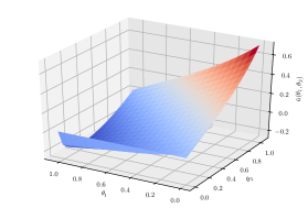
(a)

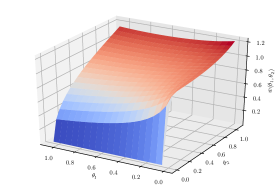
(b)

Figure 4: [Colour online] Fixed point “surfaces” for $F_{B}$ for various $\theta_{1},\theta_{2}\in(0,\pi/3)$.

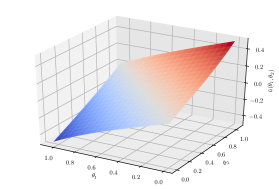
(a)

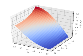
(b)

Figure 5: [Colour online] Fixed point “surfaces” for $G_{B}$ for various $\theta_{1},\theta_{2}\in(0,\pi/3)$.

3.3 Computational Results

For general dynamics, we iterated the maps (9)-(12) for 10,000 collisions for a particle always starting on $\partial\mathcal{Q}_{1}$. Initial conditions were determined using an angle $\vartheta$ which is measured anticlockwise from $\partial\mathcal{Q}_{1}$ to the forward direction of the momentum vector of the particle, as illustrated in Figure 6.

Figure 6: Graphical representation of initial conditions for computational simulation.

From this launch angle we then set $u_{0}=-\sin(\vartheta-\theta_{1})$ and $w_{0}=\cos(\vartheta-\theta_{1})$, with $y_{0}$ determined using the energy equation (7), and $x_{0}=y_{0}\tan(\theta_{1})$; using $u_{0}$ and $w_{0}$ we then determine $\bar{u}_{0}$ and $\bar{w}_{0}$ using the rotation transformation (6).

We note that there exists a reflection symmetry about the vertical axis on condition that the particle also be reflected accordingly, as illustrated in Figure 7 for $(\theta_{1},\theta_{2})=(7\pi/18,5\pi/18)$.

(a)

(b)

Figure 7: Reflection symmetry about the vertical axis in configuration space. Note that the momentum vector also needs to be reflected accordingly, otherwise a different orbit will be obtained.

This reflective symmetry corresponds to a reflection about the line $\theta_{1}=\theta_{2}$ in the parameter space. Hence we only considered parameters $\theta_{1}$, $\theta_{2}$ such that $0<\theta_{1}<\pi/2$ and $0<\theta_{2}\leq\theta_{1}$.

To illustrate the dynamics observed during simulation, we plotted the results in the dynamical system’s phase space which should not be confused with the previously defined phase space (3). We define the dynamical phase space as the set

$$\Omega\coloneqq\left\{(\bar{u},\bar{w}^{2})\in\mathbb{R}^{2}:\bar{w}^{2}\geq 0,\;\lvert\bar{u}\rvert\leq\sqrt{2E}\right\}.$$ (23)

Furthermore, the parabola

$$\Gamma_{p}\coloneqq\left\{(\bar{u},\bar{w}^{2})\in\Omega:\bar{w}^{2}>0,\;\bar{u}^{2}+\bar{w}^{2}-2E=0\right\}$$ (24)

forms the upper boundary on the phase space with the lower boundary given by

$$\Gamma_{\ell}\coloneqq\left\{(\bar{u},\bar{w}^{2})\in\Omega:\bar{w}^{2}=0,\;\lvert\bar{u}\rvert\leq\sqrt{2E}\right\}.$$ (25)

The area inclosed by $\partial\Omega\coloneqq\Gamma_{p}\cup\Gamma_{\ell}$ defines the set of allowed values that $\bar{u}$ and $\bar{w}$ may take during the particle’s motion. Points on the parabola $\Gamma_{p}$ corresponds to vertex collisions while points on the straight line $\Gamma_{\ell}$ corresponds to the particle sliding up or down the wedge walls.

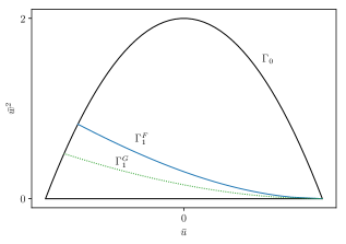
Figure 8: [Colour online] The phase space for the asymmetric wedge billiard if we follow the convention for the symmetric wedge billiard.

The lines

$$\Gamma_{1}^{F} \coloneqq\left\{(\bar{u},\bar{w}^{2})\in\Omega:(\bar{u}_{j}-2\bar{w}_{j}\cot(\theta_{1}))^{2}\right.$$

$$\qquad\left.+\bar{w}_{j}^{2}-2E=0\right\},$$ (26)

$$\Gamma_{1}^{G} \coloneqq\left\{(\bar{u},\bar{w}^{2})\in\Omega:(\bar{u}_{j}+2\bar{w}_{j}\cot(\theta_{2}))^{2}\right.$$

$$\qquad\left.+\bar{w}_{j}^{2}-2E=0\right\}$$ (27)

are the preimages of vertex collisions for the maps $F_{A}$ and $G_{A}$ respectively. We note that the lines coincide when $\theta_{1}=\theta_{2}$ and that the line $\Gamma_{1}^{F}$ lies above $\Gamma_{1}^{G}$ in the phase space $\Omega$ whenever $\theta_{1}>\theta_{2}$, as illustrated in Figure 8, and vice versa. We may suggest a division of the phase space into two or three regions possibly, as was done for the symmetric wedge billiard; however, we note that the maps (9) and (11) once again map points in $\Omega$ horizontally, which might lead to a point mapped under $F_{A}$ being beneath the line $\Gamma_{1}^{G}$ and thus possibly inferred to have been mapped there by $G_{A}$ or possibly $F_{B}$. Hence we propose that consideration should be given to a “separation” of the phase space into two copies, one indicating only collisions which occur on $\partial Q_{1}$ and the other indicating collisions which only occur on $\partial Q_{2}$, as illustrated in Figure 9.

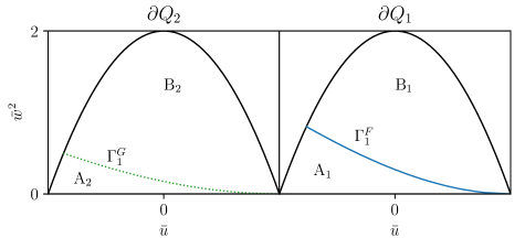
Figure 9: [Colour online] The “separated” phase space we propose for the asymmetric wedge billiard to complement the one in Figure 8.

The region $\mathrm{A}_{1}$ contains points invariant under the map $F_{A}$ and the region $\mathrm{A}_{2}$ contains points invariant under the map $G_{A}$. The region $\mathrm{B}_{1}$ contains points mapped from $\partial Q_{2}$ by the map $G_{B}$ and, similarly, the region $\mathrm{B}_{2}$ contains points mapped from $\partial Q_{1}$ by the map $F_{B}$. Hence the map $F_{B}$ maps points into either $\mathrm{A}_{2}$ or $\mathrm{B}_{2}$ and the map $G_{B}$ maps points of $\partial Q_{2}$ into either $\mathrm{A}_{1}$ or $\mathrm{B}_{1}$.

From our simulations we noted that the case $\theta_{1}+\theta_{2}=\pi/2$ is completely integrable with the phase space filled with horizontal lines, which is similar to the dynamics of the orthogonal symmetric wedge billiard [33, 34]. A complete analysis of this case will be the subject of a future article by the first author [1].

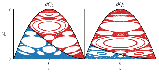
Figure 10: Phase space for $\theta_{1}=32^{\circ}$, $\theta_{2}=54^{\circ}$

Furthermore, we determined that the asymmetric wedge billiard is also completely chaotic whenever $\theta_{1}+\theta_{2}>\pi/2$ which agrees with the asymmetric wedge billiard having nonvanishing Lyapunov exponents as established by Wojtkowski [41].

For $\theta_{1}+\theta_{2}<\pi/2$ the behaviour once again varies between chaotic and quasi-periodic. However, we also noted for some parameters the phase space was completely chaotic similar to the case of $\theta_{1}+\theta_{2}>\pi/2$. We can only describe this to the broken symmetry of the asymmetric wedge and requires further investigation. Generally, for each fixed $\theta_{1}$ and $\theta_{2}$, the phase portraits had points only in $\mathrm{B}_{1}$ and $\mathrm{B}_{2}$ (see Figure 9) whenever the launch angle $\phi$ was in a neighbourhood around $\pi/2$; this corresponds to phenomena observed in the symmetric wedge billiard.

It was interesting to notice from our study of the phase portraits that the asymmetric wedge billiard also bifurcated for $\theta_{1}+\theta_{2}$ in regions close to $\arccos((\sqrt{3}-1)/2)$ and $\arccos((\sqrt{5}-1)/2)$ in correspondence with the bifurcation angles of the symmetric wedge billiard [29], even though the correspondence was not exact (see § 3.4).

3.4 Rotated Symmetric Wedge Billiard

Our model enables us to consider the case of a symmetric wedge billiard with full wedge angle rotated clockwise (or anticlockwise) from the vertical. Let

$$\omega\coloneqq\theta_{1}+\theta_{2},\qquad\gamma\coloneqq\frac{\theta_{1}-\theta_{2}}{2}$$ (28)

be the full wedge angle and rotation angle respectively, as illustrated in Figure 11. For the rest of this section we shall assume that $\omega$ and $\gamma$ are the given parameters.

fig/fig_rotated_symmetric_wedge_billiard

Figure 11: The rotated symmetric wedge billiard.

We may solve equations (28) for $\theta_{1}$, $\theta_{2}$ to obtain

$$\theta_{1}=\gamma+\frac{\omega}{2},\qquad\theta_{2}=\frac{\omega}{2}-\gamma.$$ (29)

Assume that we rotate the wedge clockwise, then it is more likely for $\theta_{2}\to 0$ before $\theta_{1}\to\pi/2$. From the physics of the model, it follows that $0<\theta_{2}<\pi/2$ and it follows from the second equation of (29) that $0<\omega/2-\gamma<\pi/2$ from which then follows $(\omega-\pi)/2<\gamma<\omega/2$. However, $(\omega-\pi)/2<0$ for $\omega\in(0,\pi/2)$ and therefore we obtain a restriction on $\gamma$ which depends on the full wedge angle $\omega$, that is, $0<\gamma<\omega/2$. Hence we may not rotate the symmetric wedge further than half its full wedge angle, which was also confirmed in our simulations.

Note that the second equation of (28) implies that $\theta_{1}>\theta_{2}$ if the rotation is clockwise. Of course, we could equally have that $\theta_{1}<\theta_{2}$ from which would then follow that $\gamma<0$ which implies anticlockwise rotation from the vertical. In this scenario, the equations in (29) become $\theta_{1}=\omega/2-\gamma$ and $\theta_{2}=\gamma+\omega/2$.

From our simulations of the rotated wedge billiard, we found that the dynamics remain close to the symmetric case for very small $\gamma$. However, as the wedge was rotated further away from the vertical, it appeared that the phase portraits were correspondingly deformed in the vertical direction of the phase diagrams. As previously stated, the bifurcation angles of the symmetric wedge billiard [29] seem to be preserved albeit not exactly. For example, for the bifurcation angle $\theta_{1}^{*}=\arccos((\sqrt{3}-1)/2)/2$ rotated $\varphi=15^{\circ}$ clockwise from the vertical, our simulations indicated that the bifurcation seems to happen at $\theta_{1}^{*}=\arccos((\sqrt{3}-1)/2)/2+5/4$. Further investigation is required to determine whether the extra term added to $\theta_{1}^{*}$ will remain a rational number and in which way it is related to the rotation angle $\gamma$.

4 Conclusion

We generalized the physical example of the wedge billiard, introduced by Lehtihet and Miller [23] and subsequently studied by Richter et al [29] and Szeredi [33, 34] amongst others, by breaking the symmetry of the wedge walls with respect to the vertical and considering two separate angles $\theta_{1}$ and $\theta_{2}$ measured with respect to the vertical.

Due to the nature of the resulting nonlinear collision maps (9)-(11), we undertook a computational study of the asymmetric wedge billiard and found that the billiard is completely chaotic when $\theta_{1}+\theta_{2}>\pi/2$, completely integrable when $\theta_{1}+\theta_{2}=\pi/2$, and varies between quasi-periodic and chaotic motions when $\theta_{1}+\theta_{2}<\pi/2$. The complete chaos observed ratifies an analytical result by Wojtkowski [41].

There are some aspects which require further study. The stability of the fixed points of $F_{B}$ and $G_{B}$ need to be determined, the authors suspect that these fixed points are unstable for all parameter values. There is also the matter of the bifurcation angles which are almost in exact correspondence with the symmetric wedge billiard. From our simulations we noted that the bifurcation occurs close to a value of the bifurcation angle of the symmetric wedge billiard, with an added rational number. We suspect that there is some relationship between this rational number and the rotation angle $\gamma$.

References

- [1] K. D. Anderson. Dynamics of a rotated orthogonal wedge billiard. Unpublished.
- [2] K. D. Anderson. Modelling and computational study of the dynamics of an asymmetric wedge billiard in a constant gravitational field. PhD thesis, University of Johannesburg, 2019.
- [3] N. Berglund and H. Kunz. Integrability and ergodicity of classical billiards in a magnetic field. Journal of Statistical Physics, 83(1-2):81–126, 1996.
- [4] M. V. Berry. Regularity and chaos in classical mechanics, illustrated by three deformations of a circular’billiard’. European Journal of Physics, 2(2):91, 1981.
- [5] G. D. Birkhoff. Dynamical systems, volume 9. American Mathematical Society, 1927.
- [6] G. D. Birkhoff. On the periodic motions of dynamical systems. Acta Mathematica, 50(1):359–379, 1927.
- [7] H. Bruus and A. D. Stone. Quantum chaos in a deformable billiard: applications to quantum dots. Physical Review B, 50(24):18275, 1994.
- [8] S. Choi, B. Sundaram, and M. Raizen. Single-photon cooling in a wedge billiard. Physical Review A, 82(3):033415, 2010.
- [9] D. R. da Costa, C. P. Dettmann, and E. D. Leonel. Circular, elliptic and oval billiards in a gravitational field. Communications in Nonlinear Science and Numerical Simulation, 22(1-3):731–746, 2015.
- [10] L. D. Da Silva and M. de Aguiar. Periodic orbits in magnetic billiards. The European Physical Journal B: Condensed Matter and Complex Systems, 16(4):719–728, 2000.
- [11] M. Deryabin and L. Pustyl’nikov. Generalized relativistic billiards. Regular and Chaotic Dynamics, 8(3):283–296, 2003.
- [12] M. Deryabin and L. Pustyl’nikov. On generalized relativistic billiards in external force fields. Letters in Mathematical Physics, 63(3):195–207, 2003.
- [13] M. Deryabin and L. Pustyl’nikov. Exponential attractors in generalized relativistic billiards. Communications in Mathematical Physics, 248(3):527–552, 2004.
- [14] A. Góngora-T, J. V. José, and S. Schaffner. Classical solutions of an electron in magnetized wedge billiards. Physical Review E, 66(4):047201, 2002.
- [15] J. M. Greene, R. MacKay, F. Vivaldi, and M. Feigenbaum. Universal behaviour in families of area-preserving maps. Physica D: Nonlinear Phenomena, 3(3):468–486, 1981.
- [16] J. H. Hale and H. Kocak. Dynamics and Bifurcations. Spring-Verlag, 1991.
- [17] A. Hartl, B. Miller, and P. Mazzoleni. Dynamics of a dissipative, inelastic gravitational billiard. Physical Review E, 87:032901, 2013.
- [18] S. Kamphorst and S. De Carvalho. Bounded gain of energy on the breathing circle billiard. Nonlinearity, 12, 1999.
- [19] J. Koiller, R. Markarian, S. Kamphorst, and S. De Carvalho. Time-dependent billiards. Nonlinearity, 8, 1995.
- [20] H. Korsch and J. Lang. A new integrable gravitational billiard. Journal of Physics A: Mathematical and General, 24(1):45, 1991.
- [21] D. G. Ladeira and J. K. L. da Silva. Scaling features of a breathing circular billiard. Journal of Physics A: Mathematical and Theoretical, 41(36):365101, 2008.
- [22] V. F. Lazutkin. The existence of caustics for a billiard problem in a convex domain. Mathematics of the USSR-Izvestiya, 7(1):185, 1973.
- [23] H. Lehtihet and B. Miller. Numerical study of a billiard in a gravitational field. Physica D: Nonlinear Phenomena, 21(1):93–104, 1986.
- [24] F. Lenz, F. K. Diakonos, and P. Schmelcher. Classical dynamics of the time-dependent elliptical billiard. Physical Review E, 76(6):066213, 2007.
- [25] F. Lenz, F. K. Diakonos, and P. Schmelcher. Scattering dynamics of driven closed billiards. EPL (Europhysics Letters), 79(2):20002, 2007.
- [26] F. Lenz, C. Petri, F. Koch, F. Diakonos, and P. Schmelcher. Evolutionary phase space in driven elliptical billiards. New Journal of Physics, 11(8):083035, 2009.
- [27] E. Piña and L. J. Lara. On the symmetry lines of the standard mapping. Physica D: Nonlinear Phenomena, 26(1-3):369–378, 1987.
- [28] H. Poritsky. The billard ball problem on a table with a convex boundary–an illustrative dynamical problem. Annals of Mathematics, 51(2):pp. 446–470, 1950.
- [29] P. H. Richter, H.-J. Scholz, and A. Wittek. A breathing chaos. Nonlinearity, 3(1):45, 1990.
- [30] M. Robnik and M. V. Berry. Classical billiards in magnetic fields. Journal of Physics A: Mathematical and General, 18(9):1361–1378, 1985.
- [31] R. Sepulchre and M. Gerard. Stabilization of periodic orbits in a wedge billiard. In 42nd IEEE International Conference on Decision and Control (IEEE Cat. No. 03CH37475), volume 2, pages 1568–1573. IEEE, 2003.
- [32] Y. G. Sinai. Dynamical systems with elastic reflections: ergodic properties of dispersing billiards. Uspekhi Matematicheskikh Nauk, 25(2):141–192, 1970.
- [33] T. Szeredi. Classical and quantum chaos in the wedge billiard. PhD thesis, McMaster University, 1993.
- [34] T. Szeredi. Hard chaos and adiabatic quantization: The wedge billiard. Journal of Statistical Physics, 83(1-2):259–274, 1996.
- [35] T. Szeredi and D. Goodings. Periodic orbits from the quantum energy spectrum of the wedge billiard. Physical Review Letters, 69(11):1640, 1992.
- [36] T. Szeredi and D. Goodings. Classical and quantum chaos of the wedge billiard. i. classical mechanics. Physical Review E, 48(5):3518, 1993.
- [37] T. Szeredi and D. Goodings. Classical and quantum chaos of the wedge billiard. ii. quantum mechanics and quantization rules. Physical Review E, 48(5):3529, 1993.
- [38] T. Tasnádi. The behavior of nearby trajectories in magnetic billiards. Journal of Mathematical Physics, 37(11):5577–5598, 1996.
- [39] H. Waalkens, J. Wiersig, and H. R. Dullin. Elliptic quantum billiard. Annals of Physics, 260(1):50–90, 1997.
- [40] M. Wojtkowski. Principles for the design of billiards with nonvanishing lyapunov exponents. Communications in Mathematical Physics, 105(3):391–414, 1986.
- [41] M. P. Wojtkowski. A system of one dimensional balls with gravity. Communications in Mathematical Physics, 126(3):507–533, 1990.