Brownian flights over a circle

Abstract

The stationary radial distribution, $P(\rho)$, of the random walk with the diffusion coefficient $D$, which winds with the tangential velocity $V$ around the impenetrable disc of radius $R$ for $R\gg 1$ converges to the distribution involving Airy function. Typical trajectories are localized in the circular strip $[R,R+\delta R^{1/3}]$, where $\delta$ is the constant which depends on the parameters $D$ and $V$ and is independent on $R$.

I Introduction

We study the behavior of the Brownian motion $B$ in $\mathbb{R}^{2}$, evading a certain region. The questions of similar nature have been considered in the literature. A notable example is the paper FS by P. Ferrari and H. Spohn, in which they discussed the limiting behavior of the directed Brownian bridge in (1+1) dimensions constrained to stay above the semicircular obstacle $D_{R}$ of the radius $R.$ It has been found in FS that the constrained Brownian trajectory in the limit $R\rightarrow\infty$ converges to a certain diffusion process, which stays at a typical distance $\sim R^{1/3}$ above $D_{R}$ and after rescaling by $R^{1/3}$ has a stationary distribution expressed in terms of the Airy function. In the later paper (ISV ) such a diffusion process (living in the halfspace $\mathbb{R}_{+}^{2}$) was named ”Ferrari-Spohn diffusion”.

Recently, in NPSVV we studied a related problem, in which the Brownian bridge is replaced by the true 2D Brownian motion, avoiding a disk (or a triangle) in $\mathbb{R}^{2}.$ The following question was the subject of the paper NPSVV : could a two-dimensional random path pushed by some constraints to an improbable ”large deviation regime”, possess extreme statistics with one-dimensional Kardar-Parisi-Zhang (KPZ) fluctuations? It has been shown that the answer is positive, though non-universal, since fluctuations depend on the underlying geometry. In NPSVV two examples of 2D systems have been considered in details: the semicircle and the triangle, for which imposed external constraints forced the underlying stationary stochastic process to stay in an atypical regime with anomalous statistics. In the paper HP the question of the behavior of a planar Brownian loop capturing a large area $A$ is studied. In particular, it has been established that a typical loop with a fixed area avoids a disc of area $\sim A$, as $A\to\infty$.

In the present paper we study a behavior of the Brownian motion $B$ in $\mathbb{R}^{2}$ which cannot enter a disc of radius $R$, moving around it with a given linear (tangential) velocity. We look at that problem from the viewpoint of the grand canonical ensemble. First of all, we find the drift field $\mathbf{v}$ (the tilt) under which the (unconstrained) Brownian particle behaves as an atypical Brownian particle winding around the disc $D_{R}$. Secondly, we determine the stationary distribution of such a particle. We find that the corresponding distribution, scaled by $R^{1/3},$ is expressed via the square of the Airy function (as $R\to\infty$) – see Eq.(37), which is the main result of our paper.

II Statement of the problem

We study large deviation problem for a biased two-dimensional Brownian motion $B$ on a plane in a radial geometry. We are looking for the rotation-invariant drift field $\mathbf{v}$, which imposes the following constraints: i) the Brownian motion always stays outside the disk $D_{R}$ of radius $R$, and ii) the Brownian motion winds around the disc with the mean angular velocity $\omega=\frac{V}{2\pi R}$ where the mean linear velocity $V$ is fixed. The requested drift field $\mathbf{v}$ should produce the same behavior as that of the Brownian particle constrained to stay away from $D_{R}$ and making a full turn around $D_{R}$ during typical time $\frac{2\pi R}{V}$. In other words, we are looking for the angular tilt which would produce the constrained behavior as its typical one. Schematically, the considered system is shown on Fig. 1.

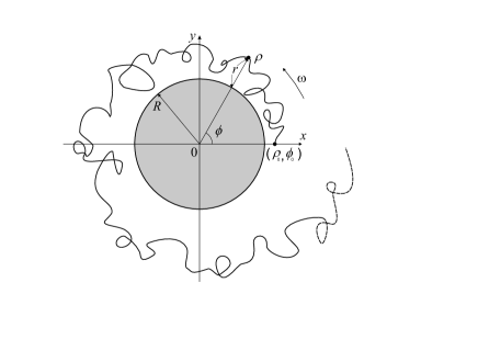
Figure 1: Schematic image of a particular realization of a two-dimensional random walk with fixed average angular velocity $\omega$ above the circle. The path starts at the point $(\rho_{0},\phi_{0})$. We are interested in finding the stationary time- and angle-independent distribution $P(\rho)$ for ensemble of such trajectories.

Our goal is to find the stationary distribution $P(\rho,\phi)$ of the process described above, where by $(\rho,\phi)$ we denote polar coordinates on the plane. Clearly, $P(\rho,\phi)=P\left(\rho\right)$, and the rotation-invariant drift field $\mathbf{v}$ is specified by its projection to one ray.

The time-dependent distribution $P(\rho,\phi,t)$ of the Brownian motion in the rotation-invariant drift field $\mathbf{v}$ satisfies the nonstationary Fokker-Planck (FP) equation, which in polar coordinates can be written as follows:

$$\frac{\partial P}{\partial t}=D\left[\frac{1}{\rho}\frac{\partial}{\partial\rho}\left(\rho\frac{\partial P}{\partial\rho}\right)+\frac{1}{\rho^{2}}\frac{\partial^{2}P}{\partial\phi^{2}}\right]-\frac{1}{\rho}\frac{\partial}{\partial\rho}\left(\rho v_{\rho}P\right)-\frac{1}{\rho}\frac{\partial}{\partial\phi}\left(v_{\phi}P\right)$$ (1)

where $v_{\phi},v_{\rho}$ are polar coordinates of the vector $\mathbf{v}(\phi,\rho)$ and $D$ is the diffusion coefficient.

Suppose the drift field $\mathbf{v}$ to be such that the corresponding diffusion $P(\rho,\phi,t)$ stays away from the disc of radius $R$, is ergodic with a stationary distribution $P(\rho,\phi)=P\left(\rho\right)$, and the prescribed mean linear velocity is $V$. Denote by $\Omega(R,V)$ the set of all corresponding drift fields $\mathbf{v}$. According to the Schilder theorem DZ ; R , the large deviation rate function for the Brownian motion is the square of the velocity. Hence the drift field $\mathbf{v}\in\Omega(R,V)$ we are looking for, is the one which minimizes the action $S$ (the ”entropy” of ensemble of Brownian trajectories)

$$S(\mathbf{v})=\int_{R}^{\infty}\mathbf{v}^{2}(\rho,\phi)P_{\mathbf{v}}(\rho,\phi)\,\rho d\rho\,d\phi$$ (2)

over $\Omega(R,V)$.

First of all, we obtain a closed expression for the action $S$ in terms of $P(\rho)$ only, expressing $v_{\rho}$ and $v_{\phi}$ as functionals of $P(\rho)$ by solving separately two auxiliary problems. Then we study the limiting behavior of the stationary distribution $P(\rho,\phi)$ as $R$ tends to the infinity, and we see the emergence of the universal distribution expressed terms of the Airy function in that limit.

II.1 Determination of radial velocity, $v_{\rho}(\rho)$

Let us point out that if $\mathbf{v}$ is rotation-invariant and $P$ is a stationary rotation-invariant solution of the equation (1), then the radial velocity $v_{\rho}(\rho)$ is defined by $P$. Indeed, the distribution $P$ and velocity $v_{\phi}$ do not depend on $t$ and $\phi$, so the Fokker-Planck (FP) equation (1) boils down to

$$D\frac{\partial}{\partial\rho}\left(\rho\frac{\partial P(\rho)}{\partial\rho}\right)-\frac{\partial}{\partial\rho}\big{(}\rho v_{\rho}P(\rho)\big{)}=0$$ (3)

Integrating the FP equation (3), we get

$$D\frac{\partial P(\rho)}{\partial\rho}=v_{\rho}P(\rho)+\frac{C_{0}}{\rho},$$ (4)

where $C_{0}$ is the integration constant, yet undetermined. Recall that $P$ is a stationary rotation-invariant distribution for which the difference $D\frac{\partial P(\rho)}{\partial\rho}-v_{\rho}P(\rho)$ vanishes since it equals to the mass transfer through the circle of radius $\rho$. Thus, the mass transfer is zero in the stationary case which implies $C_{0}=0$, and for the radial velocity one gets the expression

$$v_{\rho}(\rho)=\frac{D}{P(\rho)}\frac{\partial P(\rho)}{\partial\rho}$$ (5)

II.2 Determination of angular velocity, $v_{\phi}(\rho)$

In order to find the minimizer of the functional $S(\mathbf{v})$ of (2), we proceed as follows. First, for any distribution, $P(\rho)$, we will find the rotation-invariant velocity field, $\mathbf{v}_{P}$, which minimizes the functional

$$S_{P}\left(\mathbf{v}\right)=\int_{R}^{\infty}\int_{0}^{2\pi}v_{\phi}^{2}(\rho)P(\rho)\,\rho d\rho\,d\phi$$ (6)

Secondly, we determine the distribution $P$ which minimizes the functional $S_{P}\left(\mathbf{v}\right)$. We consider the functional $S_{P}\left(\mathbf{\ast}\right)$ in the space of velocities with the given average tangential speed, $V$, that is

$$\int_{R}^{\infty}\int_{0}^{2\pi}\frac{v_{\phi}(\rho)}{\rho}P(\rho)\,\rho d\rho\,d\phi=\frac{V}{R}$$ (7)

Collecting (6) and (7) and introducing the Lagrange multiplier, $\lambda$, we can rewrite the auxiliary minimization problem in the following form:

$$S_{P}^{\prime}=2\pi\int_{R}^{\infty}\big{(}v_{\phi}^{2}(\rho)\rho+\lambda v_{\phi}(\rho)\big{)}P(\rho)d\rho\rightarrow\mathrm{min}$$ (8)

Solution of the equation $\delta S_{P}^{\prime}=0$ gives

$$v_{\phi}(\rho)=-\frac{\lambda}{\rho}$$ (9)

Substituting (9) back into (7), we get the expression for the Lagrange multiplier $\lambda$:

$$\lambda=-\frac{V}{R}\left(2\pi\int_{R}^{\infty}\frac{P(\rho)}{\rho}d\rho\right)^{-1}$$ (10)

Thus, we find the angular velocity, $v_{\phi}\equiv\left(\mathbf{v}_{P}\right)_{\phi}$, as a functional of $P(\rho)$:

$$v_{\phi}=\frac{V}{2\pi R\rho}\left(\int_{R}^{\infty}\frac{P(\rho)}{\rho}d\rho\right)^{-1}$$ (11)

III Minimization of the action

III.1 General formalism

To find the minimizer $P(\rho)$ of the action $S$, defined in (2), we substitute (5) and (11) into (2), getting the following expression for $S\{P(\rho)\}$:

$$S\{P(\rho)\}=\int_{R}^{\infty}\big{[}v_{\rho}^{2}(\rho)+v_{\phi}(\rho)^{2}\big{]}P(\rho)\,\rho d\rho\,d\phi=2\pi\int_{R}^{\infty}\frac{D^{2}}{P(\rho)}\left(\frac{\partial P(\rho)}{\partial\rho}\right)^{2}\rho d\rho+\\ 2\pi\frac{V^{2}}{4\pi^{2}R^{2}}\int_{R}^{\infty}\frac{P(\rho)}{\rho}\left(\int_{R}^{\infty}\frac{P(\rho)}{\rho}d\rho\right)^{-2}d\rho=2\pi D^{2}\int_{R}^{\infty}\frac{1}{P(\rho)}\left(\frac{\partial P(\rho)}{\partial\rho}\right)^{2}\rho d\rho+\frac{V^{2}}{2\pi R^{2}}\left(\int_{R}^{\infty}\frac{P(\rho)}{\rho}d\rho\right)^{-1}$$ (12)

The equation for the normalization condition reads

$$\int_{R}^{\infty}\int_{0}^{2\pi}P(\rho)\,\rho d\rho\,d\phi=1,$$ (13)

Eq. (13) should be added to the action $S\{P(\rho)\}$ with the Lagrange multiplier $\gamma$.

Let us make the substitution

$$P(\rho)=Q^{2}(\rho)$$ (14)

and plug (14) into (12)–(13). We obtain the functional

$$S^{\prime}\{Q(\rho)\}=S\{Q^{2}(\rho)\}+2\pi\gamma\int_{R}^{\infty}Q^{2}(\rho)\,\rho d\rho.$$ (15)

Collecting all terms together, we can explicitly write (15) in the following form:

$$S^{\prime}\{Q(\rho)\}=8\pi D^{2}\int_{R}^{\infty}\dot{Q}^{2}\rho d\rho+\frac{V^{2}}{2\pi R^{2}}\left(\int_{R}^{\infty}\frac{Q^{2}(\rho)}{\rho}d\rho\right)^{-1}+2\pi\gamma\int_{R}^{\infty}Q^{2}(\rho)\,\rho d\rho.$$ (16)

In Eq.(16) we have used the notation $\dot{Q}=\frac{\partial Q(\rho)}{\partial\rho}$. It should be pointed out that the action (16) has the atypical second term, which, however, still allows us to proceed with the standard Euler-Lagrange minimization of the action (16). Equation $\delta S^{\prime}\{Q(\rho)\}=0$ leads to the following ordinary differential equation

$$\frac{d}{d\rho}\left(\rho\frac{dQ(\rho)}{d\rho}\right)+\left(\frac{V^{2}}{16\pi^{2}D^{2}C^{2}R^{2}\rho}-\frac{\gamma\rho}{4D^{2}}\right)Q(\rho)=0$$ (17)

where

$$C=\displaystyle\int_{R}^{\infty}\frac{P(\rho)}{\rho}d\rho$$ (18)

Developing the first term in (17), we arrive at the boundary problem

$$\begin{cases}\displaystyle\frac{d^{2}Q(\rho)}{d\rho^{2}}+\frac{1}{\rho}\frac{dQ(\rho)}{d\rho}+\frac{1}{4D^{2}}\left(\frac{V^{2}}{4\pi^{2}C^{2}R^{2}\rho^{2}}-\gamma\right)Q(\rho)=0\vskip 6.0pt plus 2.0pt minus 2.0pt\\ Q(\rho=R)=0\vskip 6.0pt plus 2.0pt minus 2.0pt\\ Q(\rho\rightarrow\infty)\rightarrow 0\end{cases}$$ (19)

The constants $C$ and $\gamma$ should be determined self-consistently. We find $Q(\rho|C,\gamma)$ by solving the boundary problem (19), then we plug $P\equiv Q^{2}(\rho|C,\gamma)$ defined in (14) into expression for $C$ getting

$$C=\int_{R}^{\infty}\frac{Q^{2}(\rho|C,\gamma)}{\rho}d\rho$$ (20)

and $\gamma$ we determine from the normalization $\int_{R}^{\infty}\rho d\rho\int_{0}^{2\pi}d\phi\,P(\rho)=1$:

$$2\pi\int_{R}^{\infty}Q^{2}(\rho|C,\gamma)\rho d\rho=1$$ (21)

III.2 Analysis of the stationary asymptotic distribution

We are interested in the asymptotic behavior of the stationary measure $P(\rho)$ in the vicinity of large circle of radius $R$, i.e. when $\rho=R+r$ and $0<r\ll R$. First, it is convenient to make in (19) the substitution $Q(\rho)=U(\rho)\rho^{-1/2}$. In terms of the function $U(\rho)$, equation (19) reads

$$\frac{d^{2}U(\rho)}{d\rho^{2}}-\frac{1}{4}\left(\frac{\gamma}{D^{2}}-\frac{\Omega^{2}}{\rho^{2}}\right)U(\rho)=0$$ (22)

where $\Omega^{2}=\displaystyle 1+\frac{V^{2}}{4\pi^{2}C^{2}D^{2}R^{2}}$. Writing $\rho=R+r$ in (22) and expanding this expression near $R$ up to linear terms in $r$, we get for $0\leq r\ll R$:

$$\left\{\begin{array}[c]{l}\displaystyle\frac{d^{2}U(r)}{dr^{2}}-\frac{1}{4}\left(\left(\frac{\gamma}{D^{2}}-\frac{\Omega^{2}}{R^{2}}\right)+\frac{2\Omega^{2}}{R^{3}}r\right)U(r)=0\vskip 6.0pt plus 2.0pt minus 2.0pt\\ U(r=0)=0\vskip 6.0pt plus 2.0pt minus 2.0pt\\ U(r\rightarrow\infty)\rightarrow 0\end{array}\right.$$ (23)

Making use of the linear transform $r=u+vx$, we rewrite the boundary problem (23) as follows

$$\begin{cases}\displaystyle\frac{d^{2}U(x)}{dx^{2}}-xU(x)=0\vskip 6.0pt plus 2.0pt minus 2.0pt\\ \displaystyle U\left(x=-\frac{u}{v}\right)=0\vskip 6.0pt plus 2.0pt minus 2.0pt\\ \displaystyle U(x\rightarrow\infty)\rightarrow 0\end{cases}$$ (24)

where

$$u=\frac{R}{2}\left(1-\frac{\gamma R^{2}}{D^{2}\Omega^{2}}\right);\qquad v=\frac{2^{1/3}R}{\Omega^{2/3}}$$ (25)

The general solution of (24)–(25) is

$$U(x)=C_{1}\,\mathrm{Ai}\left(x+a_{1}+\frac{u}{v}\right)$$ (26)

where $\displaystyle\mathrm{Ai}(x)=\frac{1}{\pi}\int_{0}^{\infty}\cos\left(\frac{t^{3}}{3}+tx\right)dt$. Hence,

$$U(r)=C_{1}\,\mathrm{Ai}\left(\frac{r-u}{v}+a_{1}+\frac{u}{v}\right)\equiv C_{1}\,\mathrm{Ai}\left(\frac{r}{v}+a_{1}\right)$$ (27)

where $C_{1}>0$ is the constant to be determined via (20) and $a_{1}\approx-2.33811$ is the first (smallest in absolute value) zero of the Airy function, i.e. the solution of the equation $\mathrm{Ai}(a_{1})=0$. Correspondingly

$$U(r)=C_{1}\,\mathrm{Ai}\left(\left(\frac{\Omega^{2}}{2}\right)^{1/3}\frac{r}{R}+a_{1}\right)\equiv C_{1}\,\mathrm{Ai}\left(\frac{\mu^{1/3}r}{R}+a_{1}\right)$$ (28)

where we have defined

$$\mu=\frac{\Omega^{2}}{2}=\frac{1}{2}\left(1+\left(\frac{V}{2\pi CDR}\right)^{2}\right)$$ (29)

Using (28) and taking into account that $Q(r)=U(r)/\sqrt{R+r}$ (where $0\leq r\ll R$), we get the explicit expression for the requested distribution function, $Q(r)$:

$$Q(r)=\frac{C_{1}}{\sqrt{R+r}}\,\mathrm{Ai}\left(\frac{\mu^{1/3}\,r}{R}+a_{1}\right)$$ (30)

The constants $C_{1},C$ are fixed by two auxiliary conditions (20) and (21), namely:

$$\displaystyle C =C_{1}^{2}\int_{0}^{\infty}\frac{dr}{(R+r)^{2}}\,\mathrm{Ai}^{2}\left(\frac{\mu^{1/3}\,r}{R}+a_{1}\right)\vskip 6.0pt plus 2.0pt minus 2.0pt$$ (31a)

$$1 =2\pi C_{1}^{2}\int_{0}^{\infty}dr\,\mathrm{Ai}^{2}\left(\frac{\mu^{1/3}\,r}{R}+a_{1}\right)$$ (31b)

Evaluating the integral in (31b), we determine the constant $C_{1}$:

$$C_{1}^{2}=\frac{\mu^{1/3}}{2\pi\left(\mathrm{Ai}^{\prime}(a_{1})\right)^{2}R};\qquad\mathrm{Ai}^{\prime}(a_{1})=\frac{d\mathrm{Ai}(x)}{dx}\bigg{|}_{x=a_{1}}$$ (32)

The constant $C$ we find perturbatively expanding the denominator in (31a) in the power series in $\frac{r}{R}\ll 1$. In the zero’s order approximation we have

$$\frac{1}{(R+r)^{2}}\approx\frac{1}{R^{2}},$$ (33)

which allows us to evaluate $C$ in (31a) in the zero’s leading term in $0\geq\frac{r}{R}\ll 1$:

$$C\approx\frac{1}{2\pi R^{2}}$$ (34)

The first-order correction to $C$ is derived in Appendix.

Collecting (30), (32) and (34), we get the final expression for the distribution function $P(\rho)$ where $\rho=R+r$:

$$P(\rho)=\frac{\mu^{1/3}}{2\pi\left(\mathrm{Ai}^{\prime}(a_{1})\right)^{2}R\,\rho}\,\mathrm{Ai}^{2}\left(\frac{\mu^{1/3}\,(\rho-R)}{R}+a_{1}\right)\qquad(\rho\geq R),$$ (35)

In (35) $\mu$ is obtained by substituting (34) into (29):

$$\mu=\frac{1}{2}\left(1+\frac{V^{2}R^{2}}{D^{2}}\right)\bigg{|}_{R\gg 1}\approx\frac{V^{2}R^{2}}{2D^{2}}.$$ (36)

IV Conclusion

We have shown in the paper that the stationary radial distribution, $P(\rho)$ of the random walk which winds with the tangential velocity $V$ around the impenetrable disc of radius $R$ for $R\gg 1$ converges to the stationary distribution involving Airy function, given by an explicit expression

$$P(\rho)=\frac{V^{2/3}}{2^{4/3}\pi\left(\mathrm{Ai}^{\prime}(a_{1})\right)^{2}D^{2/3}R^{1/3}\,\rho}\,\mathrm{Ai}^{2}\left(\left(\frac{V^{2}}{2D^{2}}\right)^{1/3}\frac{\rho-R}{R^{1/3}}+a_{1}\right)\qquad(\rho\geq R),$$ (37)

where $a_{1}\approx-2.33811$ is the first zero of the Airy function. Typical trajectories are localized in the circular strip $[R,R+\delta R^{1/3}]$, where $\delta$ is the constant which depends on the parameters $D$ and $V$ and is independent on $R$.

It should be emphasized, that the presence of the impenetrable disc which restricts Brownian flights is crucial for the asymptotic behavior (37) and for the localization of trajectories within the strip of width $R^{1/3}$. It seems instructive to compare two models which look pretty similar. The first model represents the ”stretched” random walk of $N=cR$ steps evading a disk of radius $R$ and in main respects repeats the problem considered in our paper (see also NPSVV (definitely, on has $c>4$ for the lattice version on the square lattice). The second model discussed in HP , studies the deviations from the typical ”Wulf shape” of strongly inflated random loop of $N$ steps enclosing the algebraic area $A=cN^{2}$. At $N\gg 1$ the fluctuations in the first model scale as $N^{1/3}$, while remain Gaussian with the typical width $N^{1/2}$ in the second model. In both models the trajectories are pushed to very improbable tiny regions of the phase space, however the presence of a large deviation regime seems not to be a sufficient condition to affect the statistics and the convexity of the solid boundary on which trajectories recline, is also very important.

Appendix A

Keeping the first-order corrections in (33), i.e. taking $\frac{1}{(R+r)^{2}}\approx\frac{1}{R^{2}}\left(1-\frac{2r}{R}\right)$, the selfconsistency equation (31a) becomes as follows (compare to (34))

$$C\approx\frac{C_{1}^{2}}{R^{2}}\int_{0}^{\infty}dr\,\mathrm{Ai}^{2}\left(\frac{\mu^{1/3}\,r}{R}+a_{1}\right)-\frac{2C_{1}^{2}}{R^{3}}\int_{0}^{\infty}rdr\,\mathrm{Ai}^{2}\left(\frac{\mu^{1/3}\,r}{R}+a_{1}\right)=\frac{1}{2\pi R^{2}}\left(1-\frac{4|a_{1}|}{3\pi\mu^{1/3}}\right)$$ (38)

Substituting in (38) the general expression for $\mu$ extracted from (29), we get the following equation for the constant $C$

$$2\pi CR^{2}\approx 1-\frac{2^{7/3}}{3}\frac{|a_{1}|}{\left(1+\displaystyle\frac{V^{2}}{4\pi^{2}C^{2}D^{2}R^{2}}\right)^{1/3}}$$ (39)

By definition (see (20)), the constant $C$ should be positive. Seeking the solution of (39) in the perturbative form, we may write $C$ as follows at $R\gg 1$:

$$C\approx\frac{1}{2\pi R^{2}}+\frac{\kappa_{1}}{R^{3}}+\frac{\kappa_{2}}{R^{4}}$$ (40)

where $\kappa_{1}$ and $\kappa_{2}$ are yet unknown coefficients which should be determined by solving (39) in the limit $R\gg 1$. Substituting the ansatz (40) into (39) we immediately find that $\kappa_{1}=0$ and $\kappa_{2}$ is defined by the expression

$$\kappa_{2}=-\frac{2^{4/3}}{3\pi}\frac{|a_{1}|D^{2}}{V^{2}}$$ (41)

Thus, in the first-order expansion in $r/R\ll 1$, the constant $C$, which enters in the integral (20), reads

$$C\approx\frac{1}{2\pi R^{2}}-\frac{2^{4/3}}{3\pi}\frac{|a_{1}|D^{2}}{V^{2}R^{4}}$$ (42)

References

• (1) A.Β Dembo and O.Β Zeitouni. Large Deviations Techniques and Applications. Applications of mathematics. Springer, 1998.
• (2) Ferrari, P.L. and Spohn, H., 2005. Constrained Brownian motion: fluctuations away from circular and parabolic barriers. The Annals of Probability, 33(4), pp.1302-1325.
• (3) Hammond, A. and Peres, Y., 2008. Fluctuation of a planar Brownian loop capturing a large area. Transactions of the American Mathematical Society, 360(12), pp.6197-6230.
• (4) Ioffe, D., Shlosman, S. and Velenik, Y., 2015. An invariance principle to Ferrari–Spohn diffusions. Communications in Mathematical Physics, 336(2), pp.905-932.
• (5) Nechaev, S., Polovnikov, K., Shlosman, S., Valov, A. and Vladimirov, A., 2019. Anomalous one-dimensional fluctuations of a simple two-dimensional random walk in a large-deviation regime. Physical Review E, 99(1), p.012110.
• (6) F.Β Rezakhanlou. Lectures on the large deviation principle, 1998. https://math.berkeley.edu/~rezakhan/LD.pdf