Near-linear Time Gaussian Process Optimization with
Adaptive Batching and Resparsification

Abstract

Gaussian processes (GP) are one of the most successful frameworks to model uncertainty. However, GP optimization (e.g., GP-UCB) suffers from major scalability issues. Experimental time grows linearly with the number of evaluations, unless candidates are selected in batches (e.g., using GP-BUCB) and evaluated in parallel. Furthermore, computational cost is often prohibitive since algorithms such as GP-BUCB require a time at least quadratic in the number of dimensions and iterations to select each batch.

In this paper, we introduce BBKB (Batch Budgeted Kernel Bandits), the first no-regret GP optimization algorithm that provably runs in near-linear time and selects candidates in batches. This is obtained with a new guarantee for the tracking of the posterior variances that allows BBKB to choose increasingly larger batches, improving over GP-BUCB. Moreover, we show that the same bound can be used to adaptively delay costly updates to the sparse GP approximation used by BBKB, achieving a near-constant per-step amortized cost. These findings are then confirmed in several experiments, where BBKB is much faster than state-of-the-art methods.

1 Introduction

Gaussian process (GP) optimization is a principled way to optimize a black-box function from noisy evaluations (i.e., sometimes referred to as bandit feedback). Due to the presence of noise, the optimization process is modeled as a sequential learning problem, where at each step $t$

1. the learner chooses candidate $\mathbf{x}_{t}$ out of a decision set $\mathcal{A}$;

2. the environment evaluates $f(\mathbf{x}_{t})$ and returns a noisy feedback $y_{t}$ to the learner;

3. the learner uses $y_{t}$ to guide its subsequent choices

The goal of the learner is to converge over time to a global optimal candidate. This goal is often formalized as a regret minimization problem, where the performance of the learner is evaluated by the cumulative value of the candidates chosen over time (i.e., $\sum_{t}f(\mathbf{x}_{t})$) compared to the optimum of the function $f^{\star}=\max_{\mathbf{x}}f(\mathbf{x})$. While many GP optimization algorithms come with strong theoretical guarantees and are empirically effective, most of them suffer from experimental and/or computational scalability issues.

Experimental scalability. GP optimization algorithms usually follow a sequential interaction protocol, where at each step $t$, they wait for the feedback $y_{t}$ before proposing a new candidate $\mathbf{x}_{t+1}$. As such, the experimentation time grows linearly with $t$, which may be impractical in applications where each evaluation may take long time to complete (e.g., in lab experiments). This problem can be mitigated by switching to batched algorithms, which at step $t$ propose a batch of candidates that are evaluated in parallel. After the batch is evaluated, the algorithm integrates the feedbacks and move on to select the next batch. This strategy reduces the experimentation time, but it may degrade the optimization performance, since candidates in the batch are with much less feedback. Many approaches have been proposed for batched GP optimization. Among those with theoretical guarantees, some are based on sequential greedy selection Desautels et al. [2014], entropy search Hennig & Schuler [2012], determinantal point process sampling Kathuria et al. [2016], or multi-agent cooperation Daxberger & Low [2017], as well as many heuristics for which no regret guarantees Chevalier & Ginsbourger [2013], Shah & Ghahramani [2015]. However, they all suffer from the same computational limitations of classical GP methods.

Computational scalability. The computational complexity of choosing a single candidate in classical GP methods grows quadratically with the number of evaluations. This makes it impractical to optimize complex functions, which require many steps before converging. Many approaches exist to improve scalability. Some have been proposed in the context of sequential GP optimization, such as those based on inducing points and sparse GP approximation Quinonero-Candela et al. [2007], Calandriello et al. [2019], variational inference Huggins et al. [2019], random fourier features Mutny & Krause [2018], and grid based methods Wilson & Nickisch [2015]. While some of these methods come with regret and computational guarantees, they rely on a strict sequential protocol, and therefore they are subject to the experimental bottleneck. Other scalable approximations are specific to batched methods, such as Markov approximation Daxberger & Low [2017] and Gaussian approximation Shah & Ghahramani [2015]. However, these methods fail to guarantee either low regret or scalability.

State of the art. color=yellow]General comment: we should be sure that when talking about complexity, we make it clear whether its global or per-step. GP-UCB Srinivas et al. [2010] is the most popular algorithm for GP optimization and it suffers a regret $\mathcal{O}(\sqrt{T}\gamma_{T})$ regret, where $\gamma_{T}$ is the maximal mutual information gain of a GP after $T$ evaluations Srinivas et al. [2010], Chowdhury & Gopalan [2017]. Among approximate GP optimization methods, budgeted kernelized bandits (BKB) Calandriello et al. [2019] and Thompson sampling with quadrature random features (TS-QFF) Mutny & Krause [2018] are currently the only provably scalable methods that achieve the $\mathcal{O}(\sqrt{T}\gamma_{T})$ rate with sub-cubic computational complexity. However they both fail to achieve a fully satisfactory runtime. TS-QFF’s complexity $\widetilde{\mathcal{O}}(T2^{d}d_{\text{eff}}^{2})$ scales exponentially in $d$, and therefore can only be applied to low-dimensional input spaces, while BKB’s complexity is still quadratic $\widetilde{\mathcal{O}}(T^{2}d_{\text{eff}}^{2})$. Furthermore, both TS-QFF and BKB are constrained to a sequential protocol and therefore suffer from poor experimental scalability.

In batch GP optimization, Desautels et al. [2014] introduced a batched version of GP-UCB (GP-BUCB) that can effectively deal with delayed feedback, essentially matching the rate of GP-UCB. Successive methods improved on this approach (Daxberger & Low, 2017, App. G) but are too expensive to scale and/or require strong assumptions on the function $f$ Contal et al. [2013]. Kathuria et al. [2016] uses determinantal point process (DPP) sampling to globally select the batch of points, but DPP sampling is an expensive process in itself, requiring cubic time in the number of alternatives. Although some MCMC-based approximate DPP sampler are scalable, they do not provide sufficiently strong guarantees to prove low regret. Similarly Daxberger & Low [2017] use a Markov-based approximation to select queries, but lose all regret guarantees in the process. In general, the time and space complexity of selecting each candidate $\mathbf{x}_{t}$ in the batch remains at least $\mathcal{O}(t^{2})$, resulting in an overall $\mathcal{O}(T^{3})$ time and $\mathcal{O}(T^{2})$ space complexity, which is prohibitive beyond a few thousands evaluations.

Contributions. In this paper we introduce a novel sparse approximation for batched GP-UCB, batch budgeted kernelized bandits (BBKB) with a constant $\mathcal{O}(d_{\text{eff}}^{2})$ amortized per-step complexity that can easily scale to tens of thousands of iterations.color=yellow]We should decide how to sell this “constant” claim. If $\mathcal{A}$ is finite with $A$ candidates, we prove that BBKB runs in near-linear $\widetilde{\mathcal{O}}(TAd_{\text{eff}}^{2}+Td_{\text{eff}}^{3})$ time and $\widetilde{\mathcal{O}}(Ad_{\text{eff}}^{2})$ space and it achieves a regret of order $\mathcal{O}(\sqrt{T}\gamma_{T})$, thus matching both GP-UCB and GP-BUCB at a fraction of the computational costs (i.e., their complexity scales as $O(T^{3})$). This is achieved with two new results of independent interest. First we introduce a new adaptive schedule to select the sizes of the batches of candidates, where the batches selected are larger than the ones used by GP-BUCB Desautels et al. [2014] while providing the same regret guarantees. Second we prove that the same adaptive schedule can be used to delay updates to BKB’s sparse GP approximation Calandriello et al. [2019], also without compromising regret. This results in large computational savings (i.e., from $\widetilde{\mathcal{O}}(td_{\text{eff}}^{2})$ to $\widetilde{\mathcal{O}}(d_{\text{eff}}^{2})$ per-step complexity) even in the sequential setting, since updates to the sparse GP approximation, i.e., resparsifications, are the most expensive operation performed by BKB. Delayed resparsifications also allow us to exploit important implementation optimizations in BBKB, such as rank-one updates and lazy updates of GP posterior. We also show that our approach can be combined with existing initialization procedures, both to guarantee a desired minimum level of experimental parallelism and to include pre-existing feedback to bootstrap the optimization problem. We validate our approach on several datasets, showing that BBKB matches or outperforms existing methods in both regret and runtime.

2 Preliminaries

Setting. A learner is provided with a decision set $\mathcal{A}$ (e.g., a compact set in $\mathbb{R}^{d}$) and it sequentially selects candidates $\mathbf{x}_{1},\ldots,\mathbf{x}_{T}$ from $\mathcal{A}$. At each step $t$, the learner receives a feedback $y_{t}\mathop{\overset{\mathrm{\tiny def}}{=}}f(\mathbf{x}_{t})+\eta_{t}$, where $f$ is an unknown function, and $\varepsilon_{t}$ is an additive noise drawn i.i.d. from $\mathcal{N}(0,\xi^{2})$. We denote by $\mathbf{X}_{t}\mathop{\overset{\mathrm{\tiny def}}{=}}[\mathbf{x}_{1},\dots,\mathbf{x}_{t}]^{\mathsf{\scriptscriptstyle T}}\in\mathbb{R}^{t\times d}$ the matrix of the candidates selected so far, and with $\mathbf{y}_{t}\mathop{\overset{\mathrm{\tiny def}}{=}}[y_{1},\dots,y_{t}]^{\mathsf{\scriptscriptstyle T}}$ the corresponding feedback. We evaluate the performance of the learner by its regret, i.e., $R_{T}\mathop{\overset{\mathrm{\tiny def}}{=}}\sum_{t=1}^{T}f^{\star}-f(\mathbf{x}_{t})$, where $f^{\star}=\max_{\mathbf{x}\in\mathcal{A}}f(\mathbf{x})$ is the maximum of $f$. In many applications (e.g., optimization of chemical products) it is possible to execute multiple experiments in parallel. In this case, at step $t=1$ the learner can select a batch of candidates and wait for all feedback $y_{1},..,y_{t^{\prime}}$ before moving to the next batch, starting at $t^{\prime}>t$. To relate steps with their batch, we denote by $\texttt{fb}(t)$ the index of the last step of the previous batch, i.e., at step $t$ we have access only to feedback $\mathbf{y}_{\texttt{fb}(t)}$ up to step $\texttt{fb}(t)$. Finally, $[t]=\{1,\ldots,t\}$ denotes the set of integers up to $t$.

Sparse Gaussian processes and Nyström embeddings. GPs Rasmussen & Williams [2006] are traditionally defined in terms of a mean function $\mu$, which we assume to be zero, and a covariance defined by the (bounded) kernel function $k:\mathcal{A}\times\mathcal{A}\rightarrow[0,\kappa^{2}]$. Given $\mu$, $k$, and some data, the learner can compute the posterior of the GP.

In the following we introduce the GP posterior using a formulation based on inducing points [Quinonero-Candela et al., 2007, Huggins et al., 2019], also known as sparse GP approximations, which is later convenient to illustrate our algorithm. Given a so-called dictionary of inducing points $\mathcal{S}\mathop{\overset{\mathrm{\tiny def}}{=}}\{\mathbf{x}_{i}\}_{i=1}^{m}$, let ${\mathbf{K}}_{\mathcal{S}}\in\mathbb{R}^{m\times m}$ be the kernel matrix constructed by evaluating $k(\mathbf{x}_{i},\mathbf{x}_{j})$ for all the points in $\mathcal{S}$, and similarly let $\mathbf{k}_{\mathcal{S}}(\mathbf{x})=[k(\mathbf{x}_{1},\mathbf{x}),\dots,k(\mathbf{x}_{m},\mathbf{x})]^{\mathsf{\scriptscriptstyle T}}$. Then we define a Nyström embedding as $\mathbf{z}(\cdot,\mathcal{S})\mathop{\overset{\mathrm{\tiny def}}{=}}\mathbf{K}_{\mathcal{S}}^{+/2}\mathbf{k}_{\mathcal{S}}(\cdot):\mathbb{R}^{d}\rightarrow\mathbb{R}^{m}$, where $(\cdot)^{+/2}$ indicates the square root of the pseudo-inverse. We can now introduce the matrix $\mathbf{Z}(\mathbf{X}_{t},\mathcal{S})=[\mathbf{z}(\mathbf{x}_{1},\mathcal{S}),\dots,\mathbf{z}(\mathbf{x}_{t},\mathcal{S})]^{\mathsf{\scriptscriptstyle T}}\in\mathbb{R}^{t\times m}$ containing all candidates selected so far after embedding, and define $\mathbf{V}_{t}=\mathbf{Z}(\mathbf{X}_{t},\mathcal{S})^{\mathsf{\scriptscriptstyle T}}\mathbf{Z}(\mathbf{X}_{t},\mathcal{S})+\lambda\mathbf{I}~{}\in~{}\mathbb{R}^{m\times m}$. Following Calandriello et al. [2019], the BKB approximation of the posterior mean, covariance, and variance iscolor=yellow]Is this Cala or already the original formulation of sparse GP?

$$\widetilde{\mu}_{t}(\mathbf{x}_{i},\mathcal{S})=\mathbf{z}(\mathbf{x}_{i},\mathcal{S})^{\mathsf{\scriptscriptstyle T}}\mathbf{V}_{t}^{-1}\mathbf{Z}(\mathbf{x}_{i},\mathcal{S})^{\mathsf{\scriptscriptstyle T}}\mathbf{y}_{t},$$ (1)

$$\begin{aligned} \widetilde{k}_{t}(\mathbf{x}_{i},\mathbf{x}_{j},\mathcal{S})=\tfrac{1}{\lambda}\Big{(}&k(\mathbf{x}_{i},\mathbf{x}_{j})-\mathbf{z}(\mathbf{x}_{i},\mathcal{S})^{\mathsf{\scriptscriptstyle T}}\mathbf{z}(\mathbf{x}_{j},\mathcal{S})\Big{)}+\mathbf{z}(\mathbf{x}_{i},\mathcal{S})^{\mathsf{\scriptscriptstyle T}}\mathbf{V}_{t}^{-1}\mathbf{z}(\mathbf{x}_{j},\mathcal{S}),\end{aligned}$$ (2)

$$\widetilde{\sigma}_{t}^{2}(\mathbf{x}_{i},\mathcal{S})=\widetilde{k}_{t}(\mathbf{x}_{i},\mathbf{x}_{i},\mathcal{S}),$$ (3)

where $\lambda$ is a parameter to be tuned. The subscript $t$ in $\widetilde{\mu}_{t}$ and $\widetilde{\sigma}_{t}$ indicates what we already observed (i.e., $\mathbf{X}_{t}$ and $\mathbf{y}_{t}$), and $\mathcal{S}$ indicates the dictionary used for the embedding. Moreover, if $\mathcal{S}_{\text{exact}}$ is a perfect dictionary we recover a formulation almost equivalent to the standard posterior mean and covariance of a GP, which we denote with $\mu_{t}(\mathbf{x})\mathop{\overset{\mathrm{\tiny def}}{=}}\widetilde{\mu}_{t}(\mathbf{x},\mathcal{S}_{\text{exact}})$ and $\sigma_{t}(\mathbf{x})\mathop{\overset{\mathrm{\tiny def}}{=}}\widetilde{\sigma}_{t}(\mathbf{x},\mathcal{S}_{\text{exact}})$. Examples of possible $\mathcal{S}_{\text{exact}}$ are the whole set $\mathcal{A}$ if finite, or the set of all candidates $\{\mathbf{x}_{1},\dots,\mathbf{x}_{T}\}$ selected so far.

Finally, we define the effective dimension after $t$ steps as

$$d_{\text{eff}}(\mathbf{X}_{t})=\sum_{s=1}^{t}\sigma_{t}(\mathbf{x}_{s})=\operatorname*{Tr}(\mathbf{K}_{t}(\mathbf{K}_{t}+\lambda\mathbf{I})^{-1}).$$

Intuitively, $d_{\text{eff}}(\mathbf{X}_{t})$ captures the effective number of parameters in $f$, i.e., the posterior $f$ can be represented using roughly $d_{\text{eff}}(\mathbf{X}_{t})$ coefficients. We use $d_{\text{eff}}$ to denote $d_{\text{eff}}(\mathbf{X}_{T})$ at the end of the process. Note that $d_{\text{eff}}$ is equivalent to the maximal conditional mutual information $\gamma_{T}$ of the GP Srinivas et al. [2010], up to logarithmic terms (Calandriello et al., 2017a, Lem. 1).

The GP-UCB family. GP-UCB-based algorithms aim to construct an acquisition function $u_{t}(\cdot):\mathcal{A}\to\mathbb{R}$ to act as an upper confidence bound (UCB) for the unknown function $f$. Whenever $u_{t}(\mathbf{x})$ is a valid UCB (i.e., $f(\mathbf{x})\leq u_{t}(\mathbf{x})$) and it converges to $f(\mathbf{x})$ ”sufficiently” fast, selecting candidates that are optimal w.r.t. to $u_{t}$ leads to low regret, i.e., the value $f(\mathbf{x}_{t+1})$ of $\mathbf{x}_{t+1}=\operatorname*{arg\,max}_{\mathbf{x}\in\mathcal{A}}u_{t}(\mathbf{x})$ tends to $\max_{\mathbf{x}\in\mathcal{A}}f(\mathbf{x})$ as $t$ increases.

In particular, GP-UCB Srinivas et al. [2010] defines $u_{t}(\mathbf{x})=\mu_{t}(\mathbf{x})+\beta_{t}\sigma_{t}(\mathbf{x})$. Unfortunately, GP-UCB is computationally and experimentally inefficient, as evaluating $u_{t}(\mathbf{x})$ requires $\mathcal{O}(t^{2})$ per-step and no parallel experiments are possible. To improve computations, BKB Calandriello et al. [2019] replaces $u_{t}$ with an approximate $\widetilde{u}_{t}^{\textsc{BKB}}(\mathbf{x})=\widetilde{\mu}_{t}(\mathbf{x},\mathcal{S}_{t})+\widetilde{\beta}_{t}\widetilde{\sigma}_{t}(\mathbf{x},\mathcal{S}_{t})$, which is proven to be sufficiently close to $u_{t}$ to achieve low regret. However, maintaining accuracy requires $\mathcal{O}(t)$ per step to update the dictionary $\mathcal{S}_{t}$ at each iteration, and the queries are still selected sequentially. GP-BUCB Desautels et al. [2014] tries to increase GP-UCB’s experimental efficiency by selecting a batch of queries that are all evaluated in parallel. In particular, GP-BUCB approximate the UCB as $\widetilde{u}_{t}^{\textsc{GP-BUCB}}(\mathbf{x})=\mu_{\texttt{fb}(t)}(\mathbf{x})+\beta_{t}\sigma_{t}(\mathbf{x})$, where the mean is not updated until new feedback arrives, while due to its definition the variance only depends on $\mathbf{X}_{t}$ and can be updated in an unsupervised manner. Nonetheless, GP-BUCB is as computationally slow as GP-UCB. More details about these methods are reported in Appendix A.

Controlling regret in batched Bayesian optimization. For all steps within a batch, GP-BUCB can be seen as fantasizing or hallucinating a constant feedback $\mu_{\texttt{fb}(t)}(\mathbf{x}_{t})$ so that the mean does not change, while the variances keep shrinking, thus promoting diversity in the batch. However, incorporating fantasized feedback causes ${u}^{\textsc{GP-BUCB}}_{t}$ to drift away from $u_{t}$ to the extent that it may not be a valid UCB anymore. Desautels et al. [2014] show that this issue can be managed by adjusting GP-UCB’s parameter $\beta_{t}$. In fact, it is possible to take the ${u}^{\textsc{GP-BUCB}}_{t}$ at the beginning of the batch (which is a valid UCB by definition), and correct it to hold for each hallucinated step as $f(\mathbf{x})\leq\mu_{\texttt{fb}(t)}(\mathbf{x})+\rho_{\texttt{fb}(t),t}(\mathbf{x})\beta_{\texttt{fb}(t)}\sigma_{t}(\mathbf{x}),$ where $\rho_{\texttt{fb}(t),t}(\mathbf{x})\mathop{\overset{\mathrm{\tiny def}}{=}}\frac{\sigma_{\texttt{fb}(t)}(\mathbf{x})}{\sigma_{t}(\mathbf{x})}$ is the posterior variance ratio. By using any $\alpha_{t}\geq\rho_{\texttt{fb}(t),t}(\mathbf{x})\beta_{\texttt{fb}(t)}$, we have that ${u}^{\textsc{GP-BUCB}}_{t}$ is a valid UCB. As the length of the batch increases, the ratio $\rho_{\texttt{fb}(t),t}$ may become larger, and the UCB becomes less and less tight. Crucially, the drift of the ratio can be estimated.

Proposition 1 (Desautels et al. [2014], Prop. 1).

At any step $t$, for any $\mathbf{x}\in\mathcal{A}$ the posterior ratio is bounded as

$$\rho_{\texttt{fb}(t),t}(\mathbf{x})\mathop{\overset{\mathrm{\tiny def}}{=}}\frac{\sigma_{\texttt{fb}(t)}(\mathbf{x})}{\sigma_{t}(\mathbf{x})}\leq\prod_{s=\texttt{fb}(t)+1}^{t}\left(1+\sigma_{s-1}^{2}(\mathbf{x}_{s})\right).$$

Based on this result, GP-BUCB continues the construction of the batch while $\prod_{s=\texttt{fb}(t)+1}^{t}\left(1+\sigma_{s-1}^{2}(\mathbf{x}_{s})\right)\leq C$ for some designer-defined threshold of drift $C$. Therefore, applying Proposition 2, we have that the ratio $\rho_{\texttt{fb}(t),t}(\mathbf{x})\leq C$ for any $\mathbf{x}$, and setting $\alpha_{t}\mathop{\overset{\mathrm{\tiny def}}{=}}C\beta_{\texttt{fb}(t)}$ guarantees the validity of the UCB, just as in GP-UCB. As a consequence, GP-UCB’s analysis can be leveraged to provide guarantees on the regret of GP-BUCB.

3 Efficient Batch GP Optimization

In this section, we introduce BBKB which both generalizes and improves over GP-BUCB and BKB.

0:  Set of candidates $\mathcal{A}$, $\{\widetilde{\alpha}_{t}\}_{t=1}^{T}$, $T$, $\widetilde{C}$, $\{\overline{q}_{t}\}_{t=1}^{T}$

1:  Sample $\mathbf{x}_{1}$ uniformly, receive $\mathbf{y}_{1}$

2:  Initialize $\mathcal{S}_{0}=\{\}$, $\texttt{fb}(0)=0$

3:  for $t=\{0,\dots,T-1\}$ do

4:    Select $\mathbf{x}_{t+1}=\operatorname*{arg\,max}_{\mathbf{x}\in\mathcal{A}}\widetilde{u}_{t}(\mathbf{x},\mathcal{S}_{\texttt{fb}(t)})$ 

5:    if $1+\sum_{s=\texttt{fb}(t)+1}^{t+1}\widetilde{\sigma}_{\texttt{fb}(t)}(\mathbf{x}_{s},\mathcal{S}_{\texttt{fb}(t)})\leq\widetilde{C}$ then

6:       // $\texttt{fb}(t+1)=\texttt{fb}(t)$, batch construction step

7:       Update $\widetilde{u}_{t+1}(\mathbf{x}_{t+1},\mathcal{S}_{\texttt{fb}(t+1)})$ with the new $\widetilde{\sigma}_{t+1}$

8:       Update $\widetilde{u}_{t+1}(\mathbf{x}_{i},\mathcal{S}_{\texttt{fb}(t+1)})$ for all           $\{\mathbf{x}:\widetilde{u}_{t}(\mathbf{x},\mathcal{S}_{\texttt{fb}(t)})\geq\widetilde{u}_{t+1}(\mathbf{x}_{t+1},\mathcal{S}_{\texttt{fb}(t)})\}$

9:    else

10:       // $\texttt{fb}(t+1)=t+1$, resparsification step

11:       Initialize $\mathcal{S}_{\texttt{fb}(t+1)}=\emptyset$

12:       for $\mathbf{x}_{s}\in\mathbf{X}_{\texttt{fb}(t+1)}$ do

13:          Set $\widetilde{p}_{\texttt{fb}(t+1),s}=\overline{q}_{t}\cdot\widetilde{\sigma}_{\texttt{fb}(t)}^{2}(\mathbf{x}_{s})$

14:          Draw $z_{\texttt{fb}(t+1),s}\sim Bernoulli(\widetilde{p}_{\texttt{fb}(t+1),s})$

15:          If $z_{\texttt{fb}(t+1),s}=1$, add $\mathbf{x}_{s}$ in $\mathcal{S}_{\texttt{fb}(t+1)}$

16:       end for

17:       Get feedback $\{y_{s}\}_{s=\texttt{fb}(t)+1}^{\texttt{fb}(t+1)}$

18:       Update $\widetilde{\mu}_{\texttt{fb}(t+1)}$ and $\widetilde{\sigma}_{\texttt{fb}(t+1)}$ for all $\mathbf{x}\in\mathcal{A}$

19:    end if

20:  end for

Algorithm 1 BBKB

3.1 The algorithm

The pseudocode of BBKB is presented in Algorithm 1. The dictionary is initially empty, and we have $\widetilde{\mu}_{0}(\mathbf{x})=0$ and $\widetilde{\sigma}_{0}(\mathbf{x},\{\})=k(\mathbf{x},\mathbf{x})/\lambda=\sigma_{0}(\mathbf{x})$. At each step $t$ BBKB chooses the next candidate $\mathbf{x}_{t+1}$ as the maximizer of the UCB $\widetilde{u}_{t}(\mathbf{x})=\widetilde{\mu}_{\texttt{fb}(t)}(\mathbf{x},\mathcal{S}_{\texttt{fb}(t)})+\widetilde{\alpha}_{\texttt{fb}(t)}\widetilde{\sigma}_{t}(\mathbf{x},\mathcal{S}_{\texttt{fb}(t)})$, which combines BKB and GP-BUCB’s approaches with a new element. In $\widetilde{u}_{t}$, not only we delay feedback updates as we use the posterior mean computed at the end of the last batch $\widetilde{\mu}_{\texttt{fb}(t)}$ but, unlike BKB, we keep using the same dictionary $\mathcal{S}_{\texttt{fb}(t)}$ for all steps in a batch. While freezing the dictionary leads to significantly reducing the computational complexity, delaying feedback and dictionary updates may result in poor UCB approximation. Similar to GP-BUCB, after selecting $\mathbf{x}_{t+1}$ we test the condition in (L5) to decide whether to continue the batch, a batch construction step, or not, a resparsification step. The specific formulation of our condition is crucial to guarantee near-linear runtime, and improves over the condition used in GP-BUCB. Notice that if we update dictionary and feedback at each step, BBKB reduces to BKB (up to an improved $\widetilde{\alpha}_{t}$ as discussed in the next section), while if $\mathcal{S}_{t}=\mathbf{X}_{t}$ we recover GP-BUCB, but with an improved terminating rule for batches.

In a batch construction step, we keep using the same dictionary in computing the UCBs used to select the next candidate. On the other hand, if condition (L5) determines that UCBs may become too loose, we interrupt the batch and update the sparse GP approximation, i.e., we resparsify the dictionary. To do this we employ BKB’s posterior sampling procedure in L11-16. For each candidate $\mathbf{x}_{s}$ selected so far, we compute an inclusion probability $\widetilde{p}_{\texttt{fb}(t+1),s}=\overline{q}_{t}\cdot\widetilde{\sigma}_{\texttt{fb}(t)}(\mathbf{x}_{s})$, where $\overline{q}_{t}\geq 1$ is a parameter trading-off the size of $\mathcal{S}$ and the accuracy of the approximations, and we add $\mathbf{x}_{s}$ to the new dictionary with probability $\widetilde{p}_{\texttt{fb}(t+1),s}$. A crucial difference w.r.t. BKB is that in computing the inclusion probability we use the posterior variances computed at the beginning of the batch (instead of $\widetilde{\sigma}_{\texttt{fb}(t+1)}$). While this introduces a further source of approximation, in the next section we show that this error can be controlled. The resulting dictionary is then used to compute the embedding $\mathbf{z}_{\texttt{fb}(t+1)}$ and the UCB values whenever needed.

Maximizing the UCB. To provide a meaningful Since in general $u_{t}$ is a highly non-linear, non-convex function, it may be NP-hard to compute $\mathbf{x}_{t+1}$ as its $\operatorname*{arg\,max}$ over $\mathcal{A}$. To simplify the exposition, in the rest of the paper we assume that $\mathcal{A}$ is finite with cardinality $A$ such that simple enumeration of all candidates in $\mathcal{A}$ is sufficient to exactly optimize the UCB. Both this assumption and the runtime dependency on $A$ can be easily removed if an efficient way to optimize $u_{t}$ over $\mathcal{A}$ is provided (e.g., see Mutny & Krause [2018] for the special case of $d=1$ or when $k$ is an additive kernel).

Moreover, when $\mathcal{A}$ is finite BBKB can be implemented much more efficiently. In particular, many of the quantities used by BBKB can be precomputed once at the beginning of the batch, such as pre-embedding all arms. In addition keeping the embeddings fixed during the batch allows us to update the posterior variances using efficient rank-one updates, combining the efficiency of a parametric method with the flexibility of non-parametric GPs. Finally, when both dictionary and feedback are fixed we can leverage lazy covariance evaluations, which allows us to exactly compute the $\mathbf{x}_{t+1}$ while only updating a small fraction of the UCBs (see Appendix A for more details).

3.2 Computational analysis

The global runtime of BBKB is $\mathcal{O}\big{(}TAm^{2}+BTm+B(Am^{2}+m^{3})\big{)}$, where $m=\max_{t}|\mathcal{S}_{\texttt{fb}(t)}|$ is the maximum size of the dictionary/embedding across batches, and $B$ the number of batches/resparsifications (see Appendix C for details). In order to obtain a near-linear runtime, we need to show that both $|\mathcal{S}_{t}|$ and $B$ are nearly-constant.

Theorem 1.

Given $\delta\in(0,1)$, $1\leq\widetilde{C}$, and $1\leq\lambda$, run BBKB with $\overline{q}_{t}\geq 8\log(4t/\delta)$. Then, w.p. $1-\delta$

• For all $t\in[T]$ we have $|\mathcal{S}_{t}|\leq 9\widetilde{C}(1+\kappa^{2}/\lambda)\overline{q}_{t}d_{\text{eff}}(\mathbf{X}_{t})$.

• Moreover, the total number of resparsification $B$ performed by BBKB is at most $\mathcal{O}(d_{\text{eff}}(\mathbf{X}_{t}))$.

• As a consequence, BBKB runs in near-linear time $\widetilde{\mathcal{O}}(TAd_{\text{eff}}(\mathbf{X}_{t})^{2})$ .

Theorem 1 guarantees that whenever $d_{\text{eff}}$, or equivalently $\gamma_{T}$, is near-constant (i.e., $\widetilde{\mathcal{O}}(1)$), BBKB runs in $\widetilde{\mathcal{O}}(TA)$. Srinivas et al. [2010] shows that this is the case for common kernels, e.g., $\gamma_{T}\leq\mathcal{O}(d\log(T))$ for the linear kernel and $\gamma_{T}\leq\mathcal{O}(\log(T)^{d})$ for the Gaussian kernel.

Among sequential GP-Opt algorithms, BBKB is not only much faster than the original GP-UCB $\widetilde{\mathcal{O}}(T^{3}A)$ runtime, but also much faster when compared to BKB’s quadratic $\widetilde{\mathcal{O}}(T\max\{A,T\}d_{\text{eff}}^{2})$. BBKB’s runtime also improves over GP-optimization algorithms that are specialized for stationary kernels (e.g. Gaussian), such as QFF-TS’s Mutny & Krause [2018] $\widetilde{\mathcal{O}}(TA2^{d}d_{\text{eff}}^{2})$ runtime, without making any assumption on the kernel and without an exponential dependencies on the input dimension $d$. When compared to batch algorithms, such as GP-BUCB, the improvement is even sharper as all existing batch algorithms that are provably no-regret Desautels et al. [2014], Contal et al. [2013], Shah & Ghahramani [2015] share GP-UCB’s $\widetilde{\mathcal{O}}(AT^{3})$ runtime.

color=yellow, inline]Here we should elaborate more on $d_{\text{eff}}$ and how much it can indeed change with $t$ and possibly its connection with $\gamma_{T}$ for which bounds already exist depending on the kernel.

color=yellow, inline]I would remove this whole paragraph as we have a full section on the importance of the condition and we can recall its effect there (just trying to avoid repetitions and shorten a bit the text, otherwise I would keep the paragraph). One of the central elements of this result is BBKB’s adaptive batch terminating condition. As a comparison, GP-BUCB uses $\prod_{s=\texttt{fb}(t)+1}^{t+1}(1+\sigma_{\texttt{fb}(t)}(\mathbf{x}_{s}))$ as a batch termination condition, but due to Weierstrass product inequality

$$1+\sum_{s=\texttt{fb}(t)+1}^{t+1}\sigma_{\texttt{fb}(t)}(\mathbf{x}_{s})\leq\prod_{s=\texttt{fb}(t)+1}^{t+1}(1+\sigma_{\texttt{fb}(t)}(\mathbf{x}_{s})),$$

and the product is always larger than the sum which BBKB uses. Thanks to the tighter bound, we obtain larger batches and can guarantee that at most $\widetilde{\mathcal{O}}(d_{\text{eff}})$ batches are necessary over $T$ steps. This implies that, unless $d_{\text{eff}}\to\infty$ in which case the optimization would not converge in the first place, the size of the batches must on average grow linearly with $T$ to compensate. In addition to this guarantee on the average batch size, in the next section we show how smarter initialization schemes can guarantee a minimum batch size, which is useful to fully utilize any desired level of parallelism. Finally, note that the $A$ factor reported in the runtime is pessimistic, since BBKB recomputes only a small fraction of UCB’s at each step thanks to lazy evaluations, and should be considered simply as a proxy of the time required to find the UCB maximizer.

3.3 Regret analysis

We report regret guarantees for BBKB in the so-called frequentist setting. While the algorithm uses GP tools to define and manage the uncertainty in estimating the unknown function $f$, the analysis of BBKB does not rely on any Bayesian assumption about $f$ being actually drawn from the prior $\text{GP}(0,k)$, and it only requires $f$ to be bounded in the norm associated to the RKHS induced by the kernel function $k$.

Theorem 2.

Assume $\|f\|_{\mathcal{H}}\leq F<\infty$, and let $\xi^{2}$ be the variance of the noise $\eta_{t}$. For any desired, $0<\delta<1$, $1\leq\lambda$, $1\leq\widetilde{C}$, if we run BBKB with $\overline{q}_{t}\geq 72\widetilde{C}\log(4t/\delta)$, $\widetilde{\alpha}_{\texttt{fb}(t)}=\widetilde{C}\widetilde{\beta}_{\texttt{fb}(t)}$, and

$$\widetilde{\beta}_{\texttt{fb}(t)}=2\xi \sqrt{\sum\nolimits_{s=1}^{\texttt{fb}(t)}\log\left(1+3\widetilde{\sigma}_{\texttt{fb}(s-1)}^{2}(\mathbf{x}_{s})\right)+\log\left(\tfrac{1}{\delta}\right)}$$

$$+(1+\sqrt{2})\sqrt{\lambda}F,$$

then, with prob. $1-\delta$, BBKB’s regret is bounded as

$$R_{T}^{\textsc{BBKB}} \leq 55\widetilde{C}^{2}R_{T}^{\textsc{GP-BUCB}}\leq 55\widetilde{C}^{3}R_{T}^{\textsc{GP-UCB}}$$

with $R_{T}^{\textsc{GP-UCB}}$ bounded by

$$\sqrt{T}\bigg{(}\xi\bigg{(}\sum\limits_{t=1}^{T}\sigma_{t-1}^{2}(\mathbf{x}_{t})+\log\left(\tfrac{1}{\delta}\right)\bigg{)}+\sqrt{\lambda F^{2}\sum\limits_{t=1}^{T}\sigma_{t-1}^{2}(\mathbf{x}_{t})}\bigg{)}.$$

Theorem 2 shows that BBKB achieves essentially the same regret as GP-BUCB and GP-UCB, but at a fraction of the computational cost. Note that $\sum_{t=1}^{T}\sigma_{t-1}^{2}(\mathbf{x}_{t})\approx\operatorname*{log\,det}(\mathbf{K}_{T}/\lambda+\mathbf{I})\approx\gamma_{T}$ (Srinivas et al., 2010, Lem. 5.4). Such a tight bound is achieved thanks in part to a new confidence interval radius $\widetilde{\beta}_{t}$. In particular Calandriello et al. [2019] contains an extra $\operatorname*{log\,det}(\mathbf{K}_{T}/\lambda+\mathbf{I})\leq d_{\text{eff}}(\lambda,\mathbf{X}_{T})\log(T)$ bounding step that we do not have to make. While in the worst case this is only a $\log(T)$ improvement, empirically the data adaptive bound seems to lead to much better regret.color=blued]explain a bit more why it is cool

Discussion. BBKB directly generalizes and improves both BKB and GP-BUCB. If $\widetilde{C}=1$, BBKB is equivalent to BKB, with a improved $\widetilde{\beta}_{t}$ and a slightly better regret by a factor $\log(T)$, and if $\mathcal{S}_{t}=\mathcal{S}_{\text{exact}}$ we recover GP-BUCB, with an improved batch termination rule. BBKB’s algorithmic derivation and analysis require several new tools. A direct extension of BKB to the batched setting would achieve low regret but be computationally expensive. In particular, it is easy to extend BKB’s analysis to delayed feedback, but only if BKB adapts the embedding space (i.e., resparsifies the GP) after every batch construction step to maintain guarantees at all times, i.e., Theorem 1 must hold at all steps and not only at $\texttt{fb}(t)$. However this causes large computation issues, as embedding the points is BKB’s most expensive operation, and prevents any kind of lazy evaluation of the UCBs. BBKB solves these two issues with a simple algorithmic fix by freezing the dictionary during the batch. However, this bring additional challenges for the analysis. The reason is that while the dictionary is frozen, we may encounter a point $\mathbf{x}_{t}$ that cannot be well represented with the current $S_{t}$, but we cannot add $\mathbf{x}_{t}$ to it since the dictionary is frozen. This requires studying how posterior mean and variance drift away from their values at the beginning of the batch. We tackle this problem by simultaneously freezing the dictionary and batching candidates. As we will see in the next section, and prove in the appendix, freezing the dictionary allows us to control the ratio $\widetilde{\sigma}_{\texttt{fb}(t)}(\mathbf{x}_{i},\mathcal{S}_{\texttt{fb}(t)})/\widetilde{\sigma}_{t}(\mathbf{x}_{i},\mathcal{S}_{\texttt{fb}(t)})$, obtaining a generalization of Proposition 5. However, changing the posterior mean $\widetilde{\mu}_{t}(\cdot,\mathcal{S}_{\texttt{fb}(t)})$ without changing the dictionary could still invalidate the UCBs. Batching candidates allows BBKB to continue using the posterior mean $\widetilde{\mu}_{\texttt{fb}(t)}(\cdot,\mathcal{S}_{\texttt{fb}(t)})$, which is known to be accurate, and resolve this issue. By terminating the batches when exceeding a prescribed potential error threshold (i.e., $\widetilde{C}$) we can ignore the intermediate estimate and reconnect all UCBs with the accurate UCBs at the beginning of the batch. This requires a deterministic, worst-case analysis of both the evolution of $\widetilde{\sigma}_{t}(\mathbf{x}_{i})$ and $\sigma_{t}(\mathbf{x}_{i})$, which we provide in the appendix.

Proof sketch. One of the central elements in BBKB’s computational and regret analysis is the new adaptive batch terminating condition. In particular, remember that GP-BUCB’s regret analysis was centered around the fact that the posterior ratio $\rho_{\texttt{fb}(t),t}(\mathbf{x})$ from Proposition 2 could be controlled using Desautels et al. [2014]’s batch termination rule. However, this result cannot be transferred directly to BBKB for several reasons. First, we must not only control the ratio $\rho_{\texttt{fb}(t),t}(\mathbf{x})$, but also the approximate ratio $\widetilde{\rho}_{\texttt{fb}(t),t}(\mathbf{x},\mathcal{S})\mathop{\overset{\mathrm{\tiny def}}{=}}\frac{\widetilde{\sigma}_{\texttt{fb}(t)}(\mathbf{x},\mathcal{S})}{\widetilde{\sigma}_{t}(\mathbf{x},\mathcal{S})}$ for some dictionary $\mathcal{S}$, since we are basing most of our choices on $\widetilde{\sigma}_{t}$ but will be judged based on $\sigma_{t}$ (i.e., the real function is based on $k$ and $\sigma_{t}$, not on some $\widetilde{k}$ and $\widetilde{\sigma}_{t}$). Therefore our termination rule must provide guarantees for both. Second, GP-BUCB’s rule is not only expensive to compute, but also hard to approximate. In particular, if we approximated $\sigma_{\texttt{fb}(t)}(\mathbf{x}_{s})$ with $\widetilde{\sigma}_{\texttt{fb}(t)}(\mathbf{x}_{s})$ in Proposition 2, any approximation error incurred would be compounded multiplicatively by the product resulting in an overall error exponential in the length of the batch. Instead, the following novel ratio bound involves only summations.

Lemma 1.

For any kernel $k$, dictionary $\mathcal{S}$, set of points $\mathbf{X}_{t}$, $\mathbf{x}\in\mathcal{A}$, and $\texttt{fb}(t)<t$, we have

$$\widetilde{\rho}_{\texttt{fb}(t),t}(\mathbf{x},\mathcal{S})\leq 1+\sum\nolimits_{s=\texttt{fb}(t)}^{t}\widetilde{\sigma}_{\texttt{fb}(t)}(\mathbf{x},\mathcal{S}).$$

The proof, reported in the appendix, is based only on linear algebra and does not involve any GP-specific derivation, making it applicable to the DTC approximation used by BBKB. Most importantly, it holds regardless of the dictionary $\mathcal{S}$ used (as long as it stays constant) and regardless of which candidates an algorithm might include in the batch. If we replace $\widetilde{\sigma}_{\texttt{fb}(t)}$ with $\sigma_{\texttt{fb}(t)}$ the bound can also be applied to ${\rho}_{\texttt{fb}(t),t}(\mathbf{x},\mathcal{S})$, giving us an improved version of Proposition 2 as a corollary. Finally, replacing the product in Proposition 2 with the summation in Lemma 1 makes it much easier to analyse it, leveraging this result adapted from Calandriello et al. [2019].

Lemma 2.

Under the same conditions as Theorem 1, w.p. $1-\delta$, $\forall\;\texttt{fb}(t)\in[T]$ and $\forall\;\mathbf{x}\in\mathcal{A}$ we have

$$\sigma_{\texttt{fb}(t)}^{2}(\mathbf{x})/3\leq\widetilde{\sigma}_{\texttt{fb}(t)}^{2}(\mathbf{x},\mathcal{S}_{\texttt{fb}(t)})\leq 3\sigma_{\texttt{fb}(t)}^{2}(\mathbf{x}).$$

Lemma 2 shows that at the beginning of each batch BBKB, similarly to BKB, does not underestimate uncertainty, i.e., unlike existing approximate batched methods it does not suffer from variance starvation Wang et al. [2018], Applying Lemma 2 to Lemma 1 we show that our batch terminating condition can provide guarantees on both the approximate ratio $\widetilde{\sigma}_{\texttt{fb}(t)}/\widetilde{\sigma}_{t}\leq\widetilde{C}$, as well as the exact posterior ratio $\sigma_{\texttt{fb}(t)}/\sigma_{t}\leq 3\widetilde{C}$ paying only an extra constant approximation factor. Both of these conditions are necessary to obtain the final regret bound.

color=citrine]comment related to the discussion with Daniele, about adversary screwing us —- in our setting, we are not doing contextual GPs UCB, i.e., it is the learner that is choosing $x$ unlike for PROS’N’KONS, that means we are not facing a adversary that can screw us —- yet is seems not ease to guarantee reconstructions in the middle of the batch do you agree with all this? color=blued]I agree, but i would not know how to present it

4 Extensions

In this section we discuss two important extensions of BBKB: 1) how to leverage initialization to improve experimental parallelism and accuracy, 2) how to further trade-off a small amount of extra computation to improve parallelism.

Initialization to guarantee minimum batch size. In many cases it is desirable to achieve at least a certain prescribed level of parallelism $P$, e.g., to be able to fully utilize a server farm with $P$ machines or a lab with $P$ analysis machines. However, BBKB’s batch termination rule is designed only to control the ratio error, and might generate batches smaller than $P$, especially in the beginning when posterior variances are large and their sum can quickly reach the threshold $\widetilde{C}$. However, it is easy to see that if at step $\texttt{fb}(t)$ we have $\max_{\mathbf{x}\in\mathcal{A}}\widetilde{\sigma}_{\texttt{fb}(t)}^{2}(\mathbf{x})\leq 1/P$ for all $\mathbf{x}$, then the batch will be at least as large as $P$.

The same problem of controlling the maximum posterior variance of a GP was studied by Desautels et al. [2014], who showed that a specific initialization scheme (see Appendix A for details) called uncertainty sampling (US) can guarantee that after $T_{\text{init}}$ initialization samples, we have that $\max_{\mathbf{x}\in\mathcal{A}}\sigma_{T_{\text{init}}}^{2}(\mathbf{x})\leq\gamma_{T_{\text{init}}}/T_{\text{init}}$. Since it is known that for many covariances $k$ the maximum information gain $\gamma_{t}$ grows sub-linearly in $t$, we have that $\gamma_{T_{\text{init}}}/T_{\text{init}}$ eventually reaches the desired $1/P$. For example, for the linear kernel $T_{\text{init}}\leq Pd\log(P)$ suffices, and $T_{\text{init}}\leq\log(P)^{d+1}$ for the Gaussian kernel. All of these guarantees can be transferred to our approximate setting thanks to Lemma 2 and to the monotonicity of $\sigma_{t}$. In particular, after a sufficient number $T_{\text{init}}$ of steps of US, and for any $\texttt{fb}(t)>T_{\text{init}}$ we have that

$$\widetilde{\sigma}_{\texttt{fb}(t)}(\mathbf{x},\mathcal{S}_{\texttt{fb}(t)})\leq 3\sigma_{\texttt{fb}(t)}(\mathbf{x})\leq 3\sigma_{T_{\text{init}}}(\mathbf{x})\leq 3/P,$$

and US can be used to control BBKB’s batch size as well.

Initialization to leverage existing data. In many domains GP-optimization is applied to existing problems in hope to improve performance over an existing decision system (e.g., replace uniform exploration or A/B testing with a more sophisticated alternative). In this case, existing historical data can be used to initialize the GP model and improve regret, as it is essentially “free” exploration. However this still present a computational challenge, since computing the GP posterior scales with the number of total evaluations, which includes the initialization. In this aspect, BBKB can be seamlessly integrated with initialization using pre-existing data. All that is necessary is to pre-compute a provably accurate dictionary $\mathcal{S}_{T_{\text{init}}}$ using any batch sampling technique that provides guarantees equivalent to those of Lemma 2, see e.g.,Calandriello et al. [2017a], Rudi et al. [2018]. The algorithm then continues as normal from step $T_{\text{init}}+1$ using the embeddings based on $\mathcal{S}_{T_{\text{init}}}$, maintaining all computational and regret guarantees.

Local control of posterior ratios Finally, we want to highlight that the termination rule of BBKB is just one of many possible rules to guarantee that the posterior ratio is controlled. In particular, while BBKB’s rule improves over GP-BUCB’s, it is still not optimal. For example, one could imagine recomputing all posterior variances at each step and check that $\max_{\mathbf{x}\in\mathcal{A}}\widetilde{\sigma}_{\texttt{fb}(t)}^{2}(\mathbf{x},\mathcal{S}_{\texttt{fb}(t)})/\widetilde{\sigma}_{t}^{2}(\mathbf{x},\mathcal{S}_{\texttt{fb}(t)})\leq\widetilde{C}$.

However this kind of local (i.e., specific to a $\mathbf{x}$) test is computationally expensive, as it requires a sweep over $\mathcal{A}$ and at least $\mathcal{O}(|\mathcal{S}_{\texttt{fb}(t)}|^{2})$ time to compute each variance, which is why BBKB and GP-BUCB’s termination rule use only global information. To try to combine the best of both worlds, we propose a novel efficient local termination rule.

Lemma 3.

For any kernel $k$, dictionary $\mathcal{S}$, set of points $\mathbf{X}_{t}$, $\mathbf{x}\in\mathcal{A}$, and $\texttt{fb}(t)<t$,

$$\widetilde{\rho}_{\texttt{fb}(t),t}(\mathbf{x},\mathcal{S}) \leq 1+\frac{\sum_{s=\texttt{fb}(t)}^{t}\widetilde{k}_{\texttt{fb}(t)}^{2}(\mathbf{x},\mathbf{x}_{s},\mathcal{S}_{\texttt{fb}(t)})}{\widetilde{\sigma}^{2}_{\texttt{fb}(t)}(\mathbf{x},\mathcal{S}_{\texttt{fb}(t)})}$$

Note that $\widetilde{k}_{\texttt{fb}(t)}^{2}(\mathbf{x},\mathbf{x}_{s})\leq\widetilde{\sigma}_{\texttt{fb}(t)}^{2}(\mathbf{x})\widetilde{\sigma}_{\texttt{fb}(t)}^{2}(\mathbf{x}_{s})$, due to Cauchy-Bunyakovsky-Schwarz, and therefore this termination rule is tighter than the one in Lemma 1. Moreover, with an argument similar to the one in Lemma 1 we can again show that the termination provably controls both the ratio of exact and approximate posteriors.

Computationally, after a $\widetilde{\mathcal{O}}(d_{\text{eff}}^{2})$ cost to update $\mathbf{V}_{t}^{-1}$, computing multiple $\widetilde{k}_{\texttt{fb}(t)}(\mathbf{x},\mathbf{x}_{s},\mathcal{S}_{\texttt{fb}(t)})$ for a fixed $\mathbf{x}_{s}$ requires only $\widetilde{\mathcal{O}}(d_{\text{eff}})$ time, i.e., it requires only a vector-vector multiplication in the embedded space. Therefore, the total cost of updating the posterior ratio estimates using Lemma 3 is $\widetilde{\mathcal{O}}(Ad_{\text{eff}}+d_{\text{eff}}^{2})$, while recomputing all variances requires $\mathcal{O}(Ad_{\text{eff}}^{2})$. However, it still requires a full sweep over all candidates introducing a dependency on $A$. As commented in the case of posterior maximization, lazy updates can be used to empirically alleviate this dependency. Finally, it is possible to combine both bounds: at first use the global bound from Lemma 1, and then switch to the more computationally expensive local bound of Lemma 3 only if the constructed batch is not “large enough”.

5 Experiments

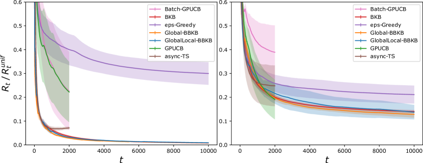
Fig. 1: Regret-ratio on Abalone (left) and Cadata (right)

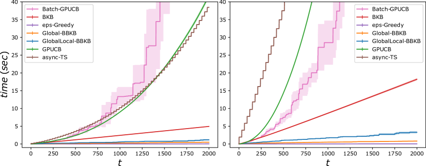
Fig. 2: Time on Abalone (left) and Cadata (right)

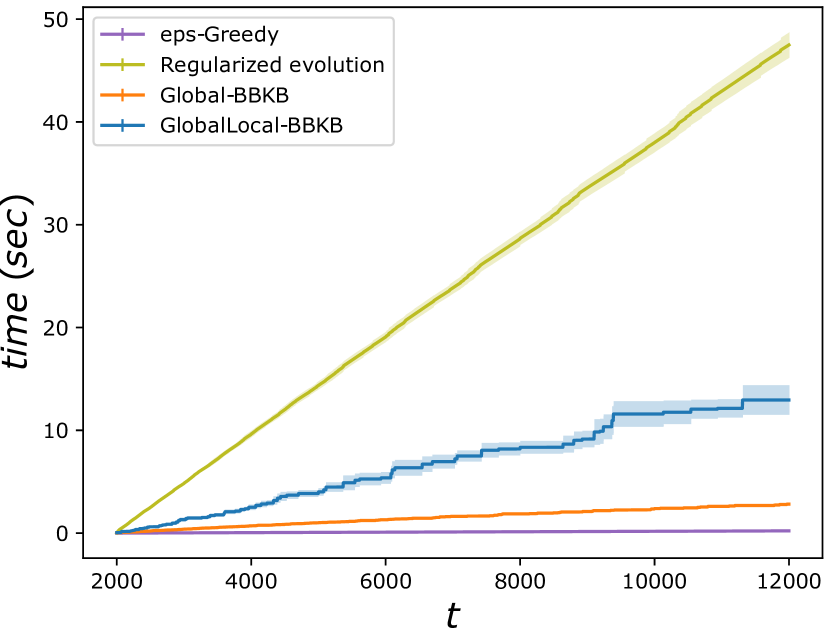
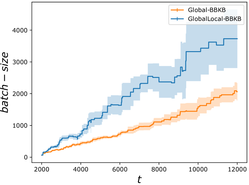
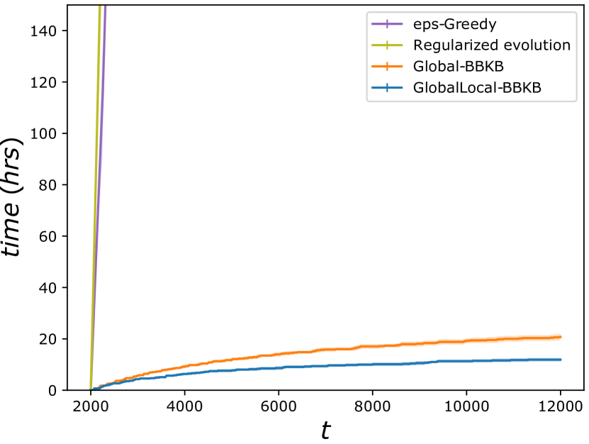
Fig. 3: From left to right time without experimental costs, batch-size and total runtime on NAS-bench-101

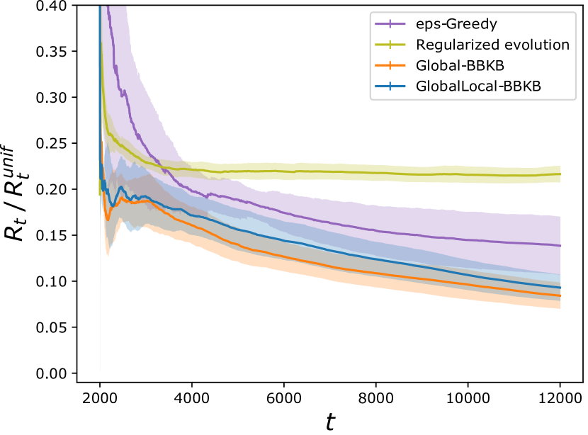
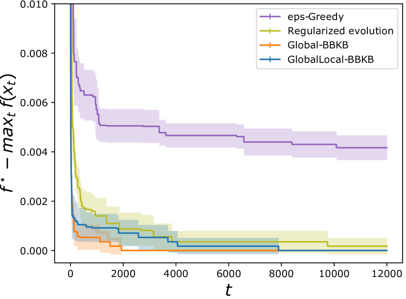
Fig. 4: From left to right regret-ratio, simple regret and simple regret without initialization on NAS-bench-101

In this section we empirically study the performance in regret and computational costs of BBKB compared to EpsGreedy, GP-UCB, GP-BUCB, BKB, batch Thompson sampling (async-TS) Kandasamy et al. [2018] and genetic algorithms (Reg-evolution) Real et al. [2019]. For BBKB we use both the batch stopping rules presented in Lemma 1 and Lemma 3 calling the two versions Global-BBKB and GlobalLocal-BBKB respectively. For each experimental result we report mean and 95% confidence interval using 10 repetitions. The experiments are implemented in python using the numpy, scikit-learn and botorch library, and run on a 16 core dual-CPU server using parallelism when allowed by the libraries. All algorithm use the hyper-parameters suggested by theory. When not applicable, cross validated parameters that perform the best for each individual algorithm are used (e.g. the kernel bandwidth). All the detailed choices and further experiments are reported in the Appendix D.

We first perform experiments on two regression datasets Abalone ($A=4177$, $d=8$) and Cadata ($A=20640$, $d=8$) datasets. We first rescale the regression target $y$ to $[0,1]$, and construct a noisy function to optimize by artificially adding a gaussian noise with zero mean and standard deviation $\xi=0.01$. For a horizon of $T=10^{4}$ iterations, we show in Figure 1 the ratio between the cumulative regret $R_{t}$ of the desired algorithm and the cumulative regret $R_{t}^{\text{unif}}$ achieved by a baseline policy that selects candidates uniformly at random. We use this metric because it is invariant to the scale of the feedback. We also report in Figure 2 the runtime of the first $2\times 10^{3}$ iterations. For both datasets, BBKB achieves the smallest regret, using only a fraction of the time of the baselines. Moreover, note that the time reported do not take into account experimentation costs, as the function is evaluated instantly.

To test how much batching can improve experimental runtime, we then perform experiments on the NAS-bench-101 dataset Ying et al. [2019], a neural network architecture search (NAS) dataset. After preprocessing we are left with $A=12416$ candidates in $d=19$ dimensions (details in Appendix D). For each candidate, the dataset contains 3 evaluations of the trained network, which we transform in a noisy function by returning one uniformly at random, and the time required to train the network. To simulate a realistic NAS scenario, we assume to start with already $T_{\text{init}}=2000$ evaluated network architectures, selected uniformly at random. Initializing BBKB using this data is straightforward. To generate an initial dictionary we use the BLESS algorithm Rudi et al. [2018], with a time cost of $2.5s$.
In Figure 3 we first report on the left the runtime of each algorithm without considering experimental costs. While both BBKB variants outperform baselines, due to the more expensive ratio estimator GlobalLocal-BBKB is slower than Global-BBKB. However, while both termination rules guarantee linearly increasing batch-sizes, we can see that the local rule outperforms the global rule. When taking into account training time, this not only shows that the batched algorithm are faster than sequential Reg-evolution, but also that GlobalLocal-BBKB with its larger batches becomes faster than Global-BBKB.

In Figure 4 we report cumulative and simple regret of BBKB against Reg-evolution, the best algorithm from Ying et al. [2019]. To measure the regret, we plot the regret ratio $R_{t}/R_{t}^{\text{unif}}$ and the simple regret (the gap between the best candidate and the best candidate found by the algorithm up to time $t$). We consider the simple regret metric because it is used in the NAS-bench-101 paper to evaluate Reg-evolution. From the plot of the regret ratio $R_{t}/R_{t}^{\text{unif}}$, we can observe how BBKB is significantly better than Reg-evolution as this latter algorithm has not been designed to minimize the cumulative regret. Further, BBKB is able to match Reg-evolution’s simple regret (the main target for this latter algorithm).

Finally, in the rightmost plot of Figure 4 we report simple regret when $T_{\text{init}}=0$ (i.e., without using initialization). Surprisingly, while the performance of Reg-evolution decreases the performance of BBKB actually increases, outperforming Reg-evolution’s. This might hint that initialization is not always beneficial in Bayesian optimization. It remains an open question to verify whether this is because the uniformly sampled initialization data makes the GP harder to approximate, or because it promotes an excessive level of exploration by increasing $\beta_{t}$ but reducing variance only in suboptimal parts of $\mathcal{A}$.

Acknowledgement
This material is based upon work supported by the Center for Brains, Minds and Machines (CBMM), funded by NSF STC award CCF-1231216, and the Italian Institute of Technology. We gratefully acknowledge the support of NVIDIA Corporation for the donation of the Titan Xp GPUs and the Tesla K40 GPU used for this research. L. R. acknowledges the financial support of the European Research Council (grant SLING 819789), the AFOSR projects FA9550-17-1-0390 and BAA-AFRL-AFOSR-2016-0007 (European Office of Aerospace Research and Development), and the EU H2020-MSCA-RISE project NoMADS - DLV-777826.

Appendix A Expanded discussion

A.1 Relationship of $\widetilde{\mu}_{t}$ and $\widetilde{\sigma}_{t}$ with Bayesian GP posteriors.

To clarify the comparison between BBKB and existing GP optimization methods, it is important to clarify the relationship between BBKB’s approximate posterior (i.e., Equations 1, 2 and 3 introduced in Calandriello et al. [2019], which we will call the BKB approximation) and the traditional definition of GP posterior commonly found in the literature (e.g., the one found in Rasmussen & Williams [2006]).

To begin, let us first consider the case of a perfect dictionary $\mathcal{S}_{\text{exact}}$ (e.g., $\mathcal{S}_{\text{exact}}=\mathcal{A}$ or $\mathcal{S}_{\text{exact}}=\mathbf{X}_{t}$). Then Equations 1, 2 and 3 can be simplified to

$$\mu_{t}\left(\mathbf{x}\;\middle|\;\mathbf{X}_{t},\mathbf{y}_{t}\right)\!=\!\mathbf{k}_{t}(\mathbf{x})^{\mathsf{\scriptscriptstyle T}}(\mathbf{K}_{t}+\lambda\mathbf{I})^{-1}\mathbf{y}_{t},$$ (4)

$$k_{t}\left(\mathbf{x},\mathbf{x}^{\prime}\;\middle|\;\mathbf{X}_{t}\right)\!=\!\tfrac{1}{\lambda}\left(k(\mathbf{x},\mathbf{x}^{\prime})-\mathbf{k}_{t}(\mathbf{x})^{\mathsf{\scriptscriptstyle T}}(\mathbf{K}_{t}+\lambda\mathbf{I})^{-1}\mathbf{k}_{t}(\mathbf{x}^{\prime})\right),$$ (5)

$$\sigma_{t}^{2}\left(\mathbf{x}\;\middle|\;\mathbf{X}_{t}\right)\!=\!k_{t}\left(\mathbf{x},\mathbf{x}\;\middle|\;\mathbf{X}_{t}\right),$$ (6)

where $\mathbf{K}_{t}\in\mathbb{R}^{t\times t}$ is the kernel matrix with $[\mathbf{K}_{t}]_{i,j}=k(\mathbf{x}_{i},\mathbf{x}_{j})$ for $\mathbf{x}_{i},\mathbf{x}_{j}$ in $\mathbf{X}_{t}$, and $\mathbf{k}_{t}(\mathbf{x})=[k(\mathbf{x}_{1},\mathbf{x}),\dots,k(\mathbf{x}_{t},\mathbf{x})]^{\mathsf{\scriptscriptstyle T}}$. Comparing this with e.g., Eq. 2.23 and 2.24 from Rasmussen & Williams [2006], which we will call $\mu_{t}^{\text{bay}}$ and $\sigma_{t}^{\text{bay}}$, we see that when $\lambda=\xi^{2}$ the definition of the posterior mean $\mu_{t}$ is identical to $\mu_{t}^{\text{bay}}$ while the posterior variance $\sigma_{t}^{\text{bay}}=\lambda\sigma_{t}=\xi^{2}\sigma_{t}$ is rescaled by a $\lambda$ factor. This rescaling is not justified in a Bayesian prior/posterior sense, and therefore $\sigma_{t}$ is not a posterior in the Bayesian sense.

However note that in the context of GP optimization with a variant of GP-UCB this distinction becomes less relevant. In particular, we are mostly interested in comparing $\beta_{t}\sigma_{t}$ against $\beta_{t}^{\text{bay}}\sigma_{t}^{\text{bay}}$ rather than simply $\sigma_{t}$ to $\sigma_{t}^{\text{bay}}$. In this case, looking at Srinivas et al. [2010] or Chowdhury & Gopalan [2017] shows that when we choose $\lambda=\xi^{2}$, then $\beta_{t}^{\text{bay}}=\beta_{t}/\lambda$, and therefore $\beta_{t}\sigma_{t}=\beta_{t}^{\text{bay}}\sigma_{t}^{\text{bay}}$. As a consequence, when $\lambda=\xi^{2}$ we can modify Calandriello et al. [2019]’s notation to match the standard Bayesian notation, and the difference becomes only a matter of simplifications. However, frequentist analysis of Kernelized-UCB algorithms show that sometimes $\lambda\neq\xi^{2}$ is the optimal choice Valko et al. [2013], and in this case the two views are not so easily reconcilable. In this paper we chose to err on the side of generality, maintaining $\lambda$ separate from $\xi^{2}$, but also on the side of familiarity and continue to refer to $\sigma_{t}$ as a posterior, with a slight abuse of terminology.

A similar argument can be made for $\widetilde{\mu}_{t}$ and $\widetilde{\sigma}_{t}$ and their Bayesian counterparts $\widetilde{\mu}_{t}^{\text{bay}}$ and $\widetilde{\sigma}_{t}^{\text{bay}}$, known as the deterministic training conditional (DTC) Quinonero-Candela et al. [2007] or projected process Seeger et al. [2003]. In particular, we have once again that the approximate posterior means $\widetilde{\mu}_{t}=\widetilde{\mu}_{t}^{\text{bay}}$ coincide, while the approximate posterior variance $\widetilde{\sigma}_{t}=\lambda\widetilde{\sigma}_{t}^{\text{bay}}$ differ by a $\lambda$ factor. Note however that although Quinonero-Candela et al. [2007] call the DTC approximation an approximate posterior, they also remark that it does not correspond to a GP posterior because it is not consistent. Therefore, regardless of the rescaling $\lambda$, it is improper to refer to the DTC or the BKB approximation as posteriors.

We choose to maintain Calandriello et al. [2019]’s notation because, as we will see in the rest of the appendix, it makes $\sigma_{t}$ coincide with the confidence intervals induced by OFUL Abbasi-Yadkori et al. [2011] and with a quantity known in randomized linear algebra as ridge leverage score Alaoui & Mahoney [2015]. Since both of these tools are crucial in our derivation, using a notation based on $\sigma_{t}^{\text{bay}}$ would require frequent rescalings by a factor $\lambda$, which although trivial might become tedious and make the exposition heavier.

A.2 Historical overview of the GP-UCB family

There are several ways to leverage a GP posterior to choose useful candidates to evaluate. Here we review those based on the GP-UCB algorithm Srinivas et al. [2010]. All GP-UCB-based algorithms rely on the construction of an acquisition function $u_{t}(\cdot):\mathcal{A}\to\mathbb{R}$ that acts as an upper confidence bound (UCB) for the unknown function $f$. Whenever $u_{t}(\mathbf{x})$ is a valid UCB (i.e., $f(\mathbf{x})\leq u_{t}(\mathbf{x})$) and it converges to $f(\mathbf{x})$ sufficiently fast, then selecting candidates that are optimal w.r.t. to $u_{t}$ leads to low regret, i.e., the value of the candidate $\mathbf{x}_{t+1}=\operatorname*{arg\,max}_{\mathbf{x}\in\mathcal{A}}u_{t}(\mathbf{x})$ tends to $\max_{\mathbf{x}\in\mathcal{A}}f(\mathbf{x})$ as $t$ increases.

GP-UCB. The original GP-UCB formulation defines the UCB as $u_{t}(\mathbf{x})=\mu_{t}(\mathbf{x})+\beta_{t}\sigma_{t}(\mathbf{x})$. An important property of this estimator is that the posterior variance is strictly non-increasing as more data is collected, i.e., $\sigma_{t+1}(\mathbf{x})\leq\sigma_{t}(\mathbf{x})$, and therefore $u_{t}(\mathbf{x})$ naturally converges to $\mu_{t}(\mathbf{x})$, which in turn tends to $f(\mathbf{x})$. Srinivas et al. [2010] found an appropriate schedule for $\beta_{t}$ that guarantees that this happens w.h.p., and that therefore $u_{t}$ is a valid UCB at all steps. However GP-UCB is computationally and experimentally slow, as evaluating $u_{t}(\mathbf{x})$ requires $\mathcal{O}(t^{2})$ per-step and no parallel experiments are possible.

BKB. A common approach to improve computational scalability in GPs is to replace the exact posterior with an approximate sparse GP posterior. The main advantage of this approximation is that if we use a dictionary $\mathcal{S}$ with size $m=|\mathcal{S}|$, then we can embed the GP in $\mathbb{R}^{m}$ using Equations 1 and 3, and keep updating the posterior in $\mathcal{O}(m^{2})$ time rather than $\mathcal{O}(t^{2})$. However, this can lead to sub-optimal choices and large regret if the dictionary $\mathcal{S}$ is not sufficiently accurate. This brings about a trade-off between larger and more accurate dictionaries, or smaller and more efficient ones. Moreover, we are only interested in approximating the part of the space that we transverse in our optimization process. Therefore, a dictionary $\mathcal{S}_{t}$ should naturally change over time to reflect which part of the space $\mathcal{A}$ is being tested. Calandriello et al. [2019] proposed to solve these problems in the BKB algorithm by replacing $u_{t}$ with an approximate version $u_{t}^{\textsc{BKB}}(\mathbf{x})=\widetilde{\mu}_{t}(\mathbf{x},\mathcal{S}_{t})+\widetilde{\beta}_{t}\widetilde{\sigma}_{t}(\mathbf{x},\mathcal{S}_{t})$, and using a procedure called posterior variance sampling (see Algorithm 1) and Calandriello et al. [2019] for more details) to update the dictionary $\mathcal{S}_{t}$ at each step. They prove that combining these approaches guarantees that ${u}_{t}^{\textsc{BKB}}$ is a UCB, and that BKB achieves low regret. However, posterior sampling requires $\mathcal{O}(t)$ per step to update the dictionary $\mathcal{S}_{t}$ at each iteration, reducing BKB’s computational scalability, and the algorithm still has poor experimental scalability since the candidates are selected sequentially.

0:  Set of candidates $\mathcal{A}$, UCB parameters $\{\alpha_{t}\}_{t=1}^{T}$, threshold $C$

  Initialize $\texttt{fb}(0)=0$

  for $t=\{0,\dots,T-1\}$ do

     Compute $\mathbf{u}_{t}^{\textsc{GP-BUCB}}(\mathbf{x})\leftarrow\mu_{\texttt{fb}(t)}(\mathbf{x})+\alpha_{t}\sigma_{t}(\mathbf{x})$

     Select $\mathbf{x}_{t+1}\leftarrow\operatorname*{arg\,max}_{\mathbf{x}\in\mathcal{A}}\mathbf{u}_{t}^{\textsc{GP-BUCB}}(\mathbf{x})$ 

     if $\prod_{s=\texttt{fb}(t)+1}^{t+1}\left(1+\sigma_{s-1}^{2}(\mathbf{x}_{s})\right)\leq{C}$ then

        $\texttt{fb}(t+1)=\texttt{fb}(t)$

        Update $\widetilde{\mathbf{u}}_{t+1}$ with the new $\widetilde{\sigma}_{t+1}$

     else

        $\texttt{fb}(t+1)=t+1$

        Get feedback $\{y_{s}\}_{s=\texttt{fb}(t)+1}^{\texttt{fb}(t+1)}$

        Update ${\mathbf{u}}_{t+1}^{\textsc{GP-BUCB}}$ with the new $\mu_{\texttt{fb}(t+1)}$ and ${\sigma}_{\texttt{fb}(t+1)}$

     end if

  end for

Algorithm 2 GP-BUCB

Batch GP-UCB. Finally, GP-BUCB Desautels et al. [2014] tries to increase GP-UCB’s experimental scalability by selecting a batch of candidates that are all evaluated in parallel. The complete structure of GP-BUCB [Desautels et al., 2014] is illustrated in Algorithm 2. GP-BUCB exploits the fact that $\sigma_{t}$ does not depend on the feedback and within a batch it defines the UCB ${u}^{\textsc{GP-BUCB}}_{t}=\mu_{\texttt{fb}(t)}(\mathbf{x})+\alpha_{t}\sigma_{t}(\mathbf{x})$, where the mean $\mu_{\texttt{fb}(t)}$ uses only the feedback up the end of the last batch, while $\sigma_{t}(\mathbf{x})$ is updated within each batch depending on the candidates until $t$. The batch is constructed by selecting candidates as $\mathbf{x}_{t+1}=\arg\max_{\mathbf{x}\in\mathcal{A}}{u}^{\textsc{GP-BUCB}}_{t}(\mathbf{x})$, then they all are evaluated in parallel, their feedback is received, and $\mu_{t}$ is updated. Notice that at the beginning of batch the UCB coincides with the one computed by GP-UCB, i.e., ${u}^{\textsc{GP-BUCB}}_{\texttt{fb}(t)}=u_{\texttt{fb}(t)}$. For all steps within a batch GP-BUCB can be seen as fantasizing or hallucinating a constant feedback $\mu_{\texttt{fb}(t)}(\mathbf{x}_{t})$ so that the mean does not change, while the variances keep shrinking, thus promoting diversity in the batch. However, incorporating fantasized feedback instead of actual feedback causes GP-BUCB’s ${u}^{\textsc{GP-BUCB}}_{t}$ criteria to drift away from $u_{t}$, which might not make it a valid UCB anymore. Desautels et al. [2014] show that this issue can be managed simply by adjusting GP-UCB’s parameter $\beta_{t}$. In fact, it is possible to take the valid h.p. GP-UCB confidence bound at the beginning of the batch, and correct it to hold for each hallucinated step as

$$f(\mathbf{x})\leq\mu_{\texttt{fb}(t)}(\mathbf{x})+\beta_{\texttt{fb}(t)}\sigma_{\texttt{fb}(t)}(\mathbf{x})\leq\mu_{\texttt{fb}(t)}(\mathbf{x})+\rho_{\texttt{fb}(t),t}(\mathbf{x})\beta_{\texttt{fb}(t)}\sigma_{t}(\mathbf{x}),$$ (7)

where $\rho_{\texttt{fb}(t),t}(\mathbf{x})\mathop{\overset{\mathrm{\tiny def}}{=}}\frac{\sigma_{\texttt{fb}(t)}(\mathbf{x})}{\sigma_{t}(\mathbf{x})}$ is the posterior variance ratio. By using any $\alpha_{t}\geq\rho_{\texttt{fb}(t),t}(\mathbf{x})\beta_{\texttt{fb}(t)}$, we have that ${u}^{\textsc{GP-BUCB}}_{t}$ is a valid UCB. As the length of the batch increases, the ratio $\rho_{\texttt{fb}(t),t}$ may become larger, and the UCB becomes less and less tight. As a result, Desautels et al. [2014] introduce an adaptive batch termination condition that ends the batch at a designer-defined level of drift $C$. Note that when selecting $C=1$ (i.e., enforcing batches of size 1) GP-BUCB reduces to the original GP-UCB. Instead of checking the ratio $\rho_{\texttt{fb}(t),t}$ for any possible candidate $\mathbf{x}$, Desautels et al. [2014] rely on the following result to derive a global condition that can be checked at any step $t$ depending only on the posterior variance computed on the candidates selected within the batch so far.

Proposition 2 ([Desautels et al., 2014], Prop. 1).

At any step $t$, let $\sigma_{\texttt{fb}(t)}$ and $\sigma_{t}$ be the posterior standard deviation at the end of the previous batch and at the current step. Then for any $\mathbf{x}\in\mathcal{A}$ their ratio is bounded as

$$\rho_{\texttt{fb}(t),t}(\mathbf{x})\mathop{\overset{\mathrm{\tiny def}}{=}}\frac{\sigma_{\texttt{fb}(t)}(\mathbf{x})}{\sigma_{t}(\mathbf{x})}\leq\prod_{s=\texttt{fb}(t)+1}^{t}\left(1+\sigma_{s-1}^{2}(\mathbf{x}_{s})\right).$$ (8)

This shows that while the standard deviation may shrink within each batch, the ratio w.r.t. the posterior at the beginning of the batch is bounded. Note that GP-BUCB continues the construction of the batch while $\prod_{s=\texttt{fb}(t)+1}^{t}\left(1+\sigma_{s-1}^{2}(\mathbf{x}_{s})\right)\leq C$ for some threshold $C$. Therefore, applying Proposition 2, we have that the ratio $\rho_{\texttt{fb}(t),t}(\mathbf{x})\leq C$ for any $\mathbf{x}$, and setting $\alpha_{t}\mathop{\overset{\mathrm{\tiny def}}{=}}C\beta_{\texttt{fb}(t)}$ guarantees the validity of the UCB. Finally, the choice of $C$ directly translates into an equivalent constant increase in the regret of GP-BUCB w.r.t. GP-UCB.

Proposition 3 (Desautels et al. [2014], Thm 2).

The regret of GP-BUCB is bounded as $R_{T}^{\textsc{GP-BUCB}}\leq CR_{T}^{\textsc{GP-UCB}}$, where $R_{T}^{\textsc{GP-UCB}}$ is the original regret of GP-UCB (see Thm. 2 for its explicit formulation).

Despite the gain in experimental parallelism and the low regret, GP-BUCB still inherits the same computational bottlenecks as GP-UCB (i.e., $O(T^{3})$ in time and $O(T^{2})$ in memory).

A.3 Lazy UCB evaluation.

Once a new dictionary is generated at the end of a batch, we compute $\mathbf{z}_{\texttt{fb}(t+1)}(\mathbf{x})$, the posterior mean and variance, and the UCB for all candidates in $\mathcal{A}$. This is an expensive operation but worth the effort, since it is done only once per batch and all subsequent computations within the batch can be done efficiently. As $\mathbf{z}(\cdot,\mathcal{S}_{\texttt{fb}(t)})$ is frozen, posterior variances can be updated using efficient rank-one updates to compute posterior variances. Furthermore, for a fixed $\mathcal{S}_{\texttt{fb}(t)}$, $\widetilde{\sigma}_{t+1}(\mathbf{x},\mathcal{S}_{\texttt{fb}(t)})\leq\widetilde{\sigma}_{t}(\mathbf{x},\mathcal{S}_{\texttt{fb}(t)})$, and since $\widetilde{\mu}_{\texttt{fb}(t)}(\mathbf{x},\mathcal{S}_{\texttt{fb}(t)})$ and $\widetilde{\alpha}_{\texttt{fb}(t)}$ remain fixed within the batch, the UCBs $\widetilde{u}_{t}(\mathbf{x},\mathcal{S}_{\texttt{fb}(t)})$ are strictly non-increasing. Therefore, after selecting $\mathbf{x}_{t+1}$ we only need to recompute $\widetilde{u}_{t+1}(\mathbf{x}_{t+1},\mathcal{S}_{\texttt{fb}(t)})$ and the UCBs for arms that had $\widetilde{u}_{t}(\mathbf{x}_{i},\mathcal{S}_{\texttt{fb}(t)})\geq\widetilde{u}_{t+1}(\mathbf{x}_{t+1},\mathcal{S}_{\texttt{fb}(t)})$ to guarantee that we are still selecting the $\operatorname*{arg\,max}$ correctly. While this lazy update of UCBs does not improve the worst-case complexity, in practice it may provide important practical speedups.

Crucially, lazy updates require that both dictionary updates and feedback are delayed during the batch. In particular, even if we do not receive new feedback simply updating the dictionary changes the embedding, and in the new representation the mean $\widetilde{\mu}_{\texttt{fb}(t)}$ and variance $\widetilde{\sigma}_{\texttt{fb}(t)}$ can both be larger or smaller, while still remaining valid. Therefore after each dictionary updates all of our UCB might be potentially the new maximizer, and we need to trigger a complete recomputation. Similarly, even if our embedding remains fixed receiving feedback can increase the mean $\widetilde{\mu}_{\texttt{fb}(t)}$ of potentially all candidates, which need to be updated. While updating all means is a slightly cheaper operation than updating the embeddings, requiring only vector-vector multiplications rather than matrix-vector multiplications, it is still an expensive operation that would prevent BBKB from achieving near-linear runtime.

A.4 Why freezing both dictionary and feedback

We remark that Lemma 1 can be immediately applied to GP-BUCB to improve it, while the application to BKB must be handled more carefully. In particular, if $\mathcal{S}=\mathcal{S}_{\text{exact}}$ then the ratios $\widetilde{\rho}_{\texttt{fb}(t),t}(\mathbf{x},\mathcal{S}_{\text{exact}})={\rho}_{\texttt{fb}(t),t}(\mathbf{x})$ coincide and as we discussed due to Weierstrass’s product inequality Lemma 1 improves on Proposition 2, resulting in an improved GP-BUCB. We can also apply Lemma 1 in two different ways to BKB. The first naive approach is to try to improve BKB’s experimental scalability through batching, i.e., use a batched UCB $\mathbf{x}_{t+1}=\operatorname*{arg\,max}_{\mathbf{x}\in\mathcal{A}}\widetilde{\mu}_{\texttt{fb}(t)}(\mathbf{x},\mathcal{S}_{t})+\widetilde{\alpha}_{t}\widetilde{\sigma}_{t}(\mathbf{x},\mathcal{S}_{t})$. However, Lemma 1 cannot be used to guarantee that this is still a valid UCB, as the dictionary changes over time. The second naive approach is to try to improve BKB’s computational scalability through dictionary freezing and adaptive resparsification, i.e., use a UCB with fixed dictionary as $\mathbf{x}_{t+1}=\operatorname*{arg\,max}_{\mathbf{x}\in\mathcal{A}}\widetilde{\mu}_{t}(\mathbf{x},\mathcal{S}_{\texttt{fb}(t)})+\widetilde{\alpha}_{\texttt{fb}(t)}\widetilde{\sigma}_{t}(\mathbf{x},\mathcal{S}_{\texttt{fb}(t)})$). However Lemma 1 only applies to the posterior variance $\widetilde{\sigma}_{t}$ and not the posterior mean $\widetilde{\mu}_{t}$, which is much harder to control. Already Calandriello et al. [2019] remark that updating the dictionary at every step is vital to guarantee that we can correctly approximate the posterior mean. Already after the first step $\texttt{fb}(t)+1$ of dictionary freezing we might be losing crucial information, e.g., $\mathbf{x}_{\texttt{fb}(t)+1}$ might be the optimal arm but if the frozen dictionary $\mathcal{S}_{\texttt{fb}(t)}$ is orthogonal to $\mathbf{x}_{\texttt{fb}(t)+1}$ we are going to ignore it until the next resparsification. Therefore, if we suspend the dictionary update for an amount of time sufficient to improve computational complexity, we might incur an equally large regret. Crucially, introducing both batching and dictionary freezing results in BBKB’s valid UCB, solving both of these problems.

A.5 Initialization and uncertainty sampling

We provide here a simplified proof of the result thanks again to our stopping rule. Let us first consider the exact case. Then if $\texttt{fb}(t)$ is the beginning of a batch and $\texttt{fb}(t^{\prime})$ the beginning of the successive batch, then the termination rule guarantees that the sum of the candidates in the batch exceeds the threshold $\sum_{s=\texttt{fb}(t)}^{\texttt{fb}(t^{\prime})}\sigma_{\texttt{fb}(t)}^{2}(\mathbf{x}_{s})\geq\widetilde{C}-1$. Therefore, if at time $\texttt{fb}(t)$ (i.e., at the beginning of a batch) we can guarantee that $\max_{\mathbf{x}}\sigma_{\texttt{fb}(t)}^{2}(\mathbf{x})\leq 1/P$, then it is easy to see that this implies

$$\widetilde{C}-1\leq\sum_{s=\texttt{fb}(t)}^{\texttt{fb}(t^{\prime})}\sigma_{\texttt{fb}(t)}^{2}(\mathbf{x}_{s})\leq\sum_{s=\texttt{fb}(t)}^{\texttt{fb}(t^{\prime})}1/P\leq(\texttt{fb}(t^{\prime})-\texttt{fb}(t))/P,$$

which implies that $\texttt{fb}(t^{\prime})-\texttt{fb}(t)\geq P(\widetilde{C}-1)$ and the batch has size at least $P(\widetilde{C}-1)$. Similarly, for the actual termination rule used by BBKB we have that $\sum_{s=\texttt{fb}(t)}^{\texttt{fb}(t^{\prime})}\widetilde{\sigma}_{\texttt{fb}(t)}^{2}(\mathbf{x}_{s},\mathcal{S}_{\texttt{fb}(t)})\geq\widetilde{C}-1$. Since each different dictionary might result in slightly different lower bounds for the batch size, we can use Lemma 2 to bring ourselves back to the exact case

$$\widetilde{C}-1\leq\sum_{s=\texttt{fb}(t)}^{\texttt{fb}(t^{\prime})}\widetilde{\sigma}_{\texttt{fb}(t)}^{2}(\mathbf{x}_{s},\mathcal{S}_{\texttt{fb}(t)})\leq 3\sum_{s=\texttt{fb}(t)}^{\texttt{fb}(t^{\prime})}\sigma_{\texttt{fb}(t)}^{2}(\mathbf{x}_{s})\leq 3(\texttt{fb}(t^{\prime})-\texttt{fb}(t))/P,$$

and therefore $\texttt{fb}(t^{\prime})-\texttt{fb}(t)\geq P(\widetilde{C}-1)/3$. All that is left is to guarantee that $\max_{\mathbf{x}}\sigma_{\texttt{fb}(t)}^{2}(\mathbf{x})\leq 1/P$.

0:  Arm set $\mathcal{A}$, $P$

0:  Init. set $\mathbf{X}_{T_{\text{init}}}$

  Select $\mathbf{x}_{1}\leftarrow\operatorname*{arg\,max}_{\mathbf{x}_{i}\in\mathcal{A}}\sigma_{0}(\mathbf{x}_{i})$

  $T_{\text{init}}\leftarrow 1$

  while $\sigma_{T_{\text{init}}-1}(\mathbf{x}_{T_{\text{init}}})\geq 1/P$ do

     $T_{\text{init}}\leftarrow T_{\text{init}}+1$

     Select $\mathbf{x}_{T_{\text{init}}}\leftarrow\operatorname*{arg\,max}_{\mathbf{x}_{i}\in\mathcal{A}}\sigma_{T_{\text{init}}-1}(\mathbf{x}_{i})$

     Update all $\sigma_{T_{\text{init}}}(\mathbf{x})$ with $\mathbf{x}_{T_{\text{init}}}$

  end while

Algorithm 3 Uncertainty sampling

First we remark that since $\sigma_{t}$ is non-increasing, the batch sizes (up to small fluctuations due to GP approximation), will also be non-decreasing over time. We can then use this intuition to see that selecting beforehand an initial set of $T_{\text{init}}$ candidates to force $\max_{\mathbf{x}}\sigma_{T_{\text{init}}}^{2}(\mathbf{x})\leq 1/P$ is sufficient to guarantee the minimum batch size for the whole optimization process. For this purpose, we can use (Desautels et al., 2014, Lem. 4).

Proposition 4 ((Desautels et al., 2014, Lem. 4)).

Given the uncertainty sampling procedure reported in Algorithm 3, we have $\max_{\mathbf{x}\in\mathcal{A}}\sigma_{T_{\text{init}}}^{2}(\mathbf{x})\leq\gamma_{T_{\text{init}}}/T_{\text{init}}$.

Combining this with the bounds on $\gamma_{T_{\text{init}}}$ reported in Desautels et al. [2014] we can guarantee a minimum degree of experimental parallelism for BBKB.

Appendix B Controlling posterior ratios

In this section we collect most results related to providing guarantees that exact and approximate posteriors remain close during the whole optimization process.

B.1 Preliminary results

Several results presented in this appendix are easier to express and prove using the so-called feature-space view of a GP Rasmussen & Williams [2006]. In particular, to every covariance $k(\cdot,\cdot)$ and reproducing kernel Hilbert space $\mathcal{H}$ we can associate a feature map $\boldsymbol{\phi}(\cdot)$ such that $k(\mathbf{x}_{i},\mathbf{x}_{j})=\boldsymbol{\phi}(\mathbf{x}_{i})^{\mathsf{\scriptscriptstyle T}}\boldsymbol{\phi}(\mathbf{x}_{j})$, and that $k(\mathbf{x}_{i},\mathbf{x}_{i})=\boldsymbol{\phi}(\mathbf{x}_{i})^{\mathsf{\scriptscriptstyle T}}\boldsymbol{\phi}(\mathbf{x}_{i})=\|\boldsymbol{\phi}(\mathbf{x}_{i})\|^{2}$. Let $\boldsymbol{\Phi}(\mathbf{X}_{t})=[\boldsymbol{\phi}(\mathbf{x}_{1}),\dots,\boldsymbol{\phi}(\mathbf{x}_{t})]^{\mathsf{\scriptscriptstyle T}}$ be the map where each row corresponds to a row of the matrix $\mathbf{X}_{t}$ after the application of $\boldsymbol{\phi}(\cdot)$. Finally, given operator $\mathbf{A}$, we use $\|\mathbf{A}\|$ to indicate its $\ell_{2}$ operator norm, also known as sup norm. For symmetric positive semi-definite matrices, this corresponds simply to its largest eigenvalue.

Using the feature-space view of a GP we can introduce an important reformulation of the posterior variance $\sigma_{t}^{2}(\mathbf{x}_{i})$

$$\sigma^{2}_{t}(\mathbf{x}_{i})=\boldsymbol{\phi}(\mathbf{x}_{i})^{\mathsf{\scriptscriptstyle T}}(\boldsymbol{\Phi}(\mathbf{X}_{t})^{\mathsf{\scriptscriptstyle T}}\boldsymbol{\Phi}(\mathbf{X}_{t})+\lambda\mathbf{I})^{-1}\boldsymbol{\phi}(\mathbf{x}_{i}).$$

In particular, this quadratic form is well known in randomized numerical linear algebra as ridge leverage scores (RLS) Alaoui & Mahoney [2015], and used extensively in linear sketching algorithms Woodruff et al. [2014]. Therefore, some of the results we will present now are inspired from this parallel literature. For example the proof of Lemma 2, restated here for convenience, is based on concentration results for RLS sampling. See 2

Proof.

We briefly show here that we can apply Calandriello et al. [2019, Thm. 1]’s result from sequential RLS sampling to our batch setting. In particular, (Calandriello et al., 2019, Thm. 1) gives identical guarantees as Lemma 2, but only when the dictionary is resparsified at each step, and we must compensate for the delays.

At a high level, their result shows that given a so-called $(\varepsilon,\lambda)$-accurate dictionary $\mathcal{S}_{t}$ it is possible to sample a $(\varepsilon,\lambda)$-accurate dictionary $\mathcal{S}_{t+1}$ using the posterior variance estimator $\widetilde{\sigma}_{t}(\mathbf{x},\mathcal{S}_{t})$ from Equation 3. Since all other guarantees directly follow from $(\varepsilon,\lambda)$-accuracy, we only need to show that the same inductive argument holds if we apply it on a batch-by-batch basis instead of a step-by-step basis. To simplify, we will also only consider the case $\varepsilon=1/2$. For more details, we refer the reader to the whole proof in (Calandriello et al., 2019, App. C).

In particular, consider the state of the algorithm at the beginning of the first batch, i.e., just after initialization ended. Since the subset $\mathcal{S}_{1}=\mathbf{X}_{1}$ includes all arms pulled so far (i.e., $\mathbf{x}_{1}$) it clearly perfectly preserves $\mathbf{X}_{1}$, and is therefore infinitely accurate and also $(1/2,\lambda)$-accurate. Note that Calandriello et al. [2019] make the same reasoning for their base case.

Thereafter, assume that $\mathcal{S}_{\texttt{fb}(t)}$ is $(1/2,\lambda)$-accurate, and let $t^{\prime}>\texttt{fb}(t)$ be the time step where we resparsify the dictionary (i.e., the beginning of the following batch) such that $\texttt{fb}(t^{\prime}-1)=\texttt{fb}(t)$ and $\texttt{fb}(t^{\prime})=t^{\prime}$. To guarantee that $\mathcal{S}_{\texttt{fb}(t^{\prime})}$ is also $(1/2,\lambda)$-accurate we must guarantee that the probabilities $\widetilde{p}_{\texttt{fb}(t^{\prime})}$ used to sample are at least as large as the true posterior $\sigma_{\texttt{fb}(t^{\prime})}^{2}$ scaled by a factor $24\log(4T/\delta)$, i.e., $\widetilde{p}_{\texttt{fb}(t^{\prime})}\geq(24\log(4T/\delta))\cdot\sigma_{\texttt{fb}(t^{\prime})}$. From the inductive assumption we know that $\mathcal{S}_{\texttt{fb}(t)}$ is $(1/2,\lambda)$-accurate, and therefore Lemma 2 holds and $\widetilde{\sigma}_{\texttt{fb}(t)}\geq\sigma_{\texttt{fb}(t)}/3\geq\sigma_{\texttt{fb}(t^{\prime})}^{2}/3$, since it is a well known property of RLS and $\sigma_{t}$ that they are non-increasing in $t$ Calandriello et al. [2017b]. Adjusting $\overline{q}$ to match this condition, we guarantee that we are sampling at least as much as required by Calandriello et al. [2019], and therefore achieve the same accuracy guarantees. ∎

B.2 Global ratio bound

Before moving on to Lemma 1 and Lemma 6, we will first consider exact posterior variances $\sigma_{t}^{2}(\mathbf{x}_{i})$, which represent a simpler case since we do not have to worry about the presence of a dictionary. The following Lemma will form a blueprint for the derivation of Lemma 1.

Lemma 4.

For any kernel $k$, set of points $\mathbf{X}_{t}$, $\mathbf{x}_{i}\in\mathcal{A}$, and $\texttt{fb}(t)<t$,

$$\sigma^{2}_{{t}}(\mathbf{x}_{i})\leq\sigma^{2}_{\texttt{fb}(t)}(\mathbf{x}_{i})\leq\left(1+\sum_{s=\texttt{fb}(t)+1}^{t}\sigma^{2}_{\texttt{fb}(t)}(\mathbf{x}_{s})\right)\sigma^{2}_{t}(\mathbf{x}_{i})$$

Proof.

Denote with $\mathbf{A}=\boldsymbol{\Phi}(\mathbf{X}_{\texttt{fb}(t)})^{\mathsf{\scriptscriptstyle T}}\boldsymbol{\Phi}(\mathbf{X}_{\texttt{fb}(t)})+\lambda\mathbf{I}$, and with $\mathbf{B}=\boldsymbol{\Phi}(\mathbf{X}_{[\texttt{fb}(t)+1,t]})$ the concatenation of only the arms between rows $\texttt{fb}(t)+1$ and $t$, i.e., in the context of BBKB $\boldsymbol{\Phi}(\mathbf{X}_{[\texttt{fb}(t)+1,t]})$ contains the arms in the current batch whose feedback has not been received yet. Then we have $\sigma^{2}_{\texttt{fb}(t)}(\mathbf{x}_{i})=\boldsymbol{\phi}(\mathbf{x}_{i})^{\mathsf{\scriptscriptstyle T}}\mathbf{A}^{-1}\boldsymbol{\phi}(\mathbf{x}_{i})$ and

$$\sigma^{2}_{t}(\mathbf{x}_{i})=\boldsymbol{\phi}(\mathbf{x}_{i})^{\mathsf{\scriptscriptstyle T}}\left(\boldsymbol{\Phi}(\mathbf{X}_{t})^{\mathsf{\scriptscriptstyle T}}\boldsymbol{\Phi}(\mathbf{X}_{t})+\lambda\mathbf{I}\right)^{-1}\boldsymbol{\phi}(\mathbf{x}_{i})=\boldsymbol{\phi}(\mathbf{x}_{i})^{\mathsf{\scriptscriptstyle T}}\left(\mathbf{A}+\mathbf{B}^{\mathsf{\scriptscriptstyle T}}\mathbf{B}\right)^{-1}\boldsymbol{\phi}(\mathbf{x}_{i}),$$

We can now collect $\mathbf{A}$ to obtain

$$\sigma^{2}_{t}(\mathbf{x}_{i}) =\boldsymbol{\phi}(\mathbf{x}_{i})^{\mathsf{\scriptscriptstyle T}}(\mathbf{A}+\mathbf{B}^{\mathsf{\scriptscriptstyle T}}\mathbf{B})^{-1}\boldsymbol{\phi}(\mathbf{x}_{i})=\boldsymbol{\phi}(\mathbf{x}_{i})^{\mathsf{\scriptscriptstyle T}}\mathbf{A}^{-1/2}(\mathbf{I}+\mathbf{A}^{-1/2}\mathbf{B}^{\mathsf{\scriptscriptstyle T}}\mathbf{B}\mathbf{A}^{-1/2})^{-1}\mathbf{A}^{-1/2}\boldsymbol{\phi}(\mathbf{x}_{i})$$

$$\geq\lambda_{\min}\left((\mathbf{I}+\mathbf{A}^{-1/2}\mathbf{B}^{\mathsf{\scriptscriptstyle T}}\mathbf{B}\mathbf{A}^{-1/2})^{-1}\right)\boldsymbol{\phi}(\mathbf{x}_{i})^{\mathsf{\scriptscriptstyle T}}\mathbf{A}^{-1}\boldsymbol{\phi}(\mathbf{x}_{i})$$

$$=\lambda_{\min}\left((\mathbf{I}+\mathbf{A}^{-1/2}\mathbf{B}^{\mathsf{\scriptscriptstyle T}}\mathbf{B}\mathbf{A}^{-1/2})^{-1}\right)\sigma_{\texttt{fb}(t)}(\mathbf{x}_{i}).$$

Focusing on the first part

$$\lambda_{\min}\left((\mathbf{I}+\mathbf{A}^{-1/2}\mathbf{B}^{\mathsf{\scriptscriptstyle T}}\mathbf{B}\mathbf{A}^{-1/2})^{-1}\right) =\frac{1}{\lambda_{\max}\left(\mathbf{I}+\mathbf{A}^{-1/2}\mathbf{B}^{\mathsf{\scriptscriptstyle T}}\mathbf{B}\mathbf{A}^{-1/2}\right)}$$

$$=\frac{1}{1+\lambda_{\max}(\mathbf{A}^{-1/2}\mathbf{B}^{\mathsf{\scriptscriptstyle T}}\mathbf{B}\mathbf{A}^{-1/2})}=\frac{1}{1+\lambda_{\max}(\mathbf{B}\mathbf{A}^{-1}\mathbf{B}^{\mathsf{\scriptscriptstyle T}})}.$$

Expanding the definition of $\mathbf{B}$, and using $\lambda_{\max}(\mathbf{B}\mathbf{A}^{-1}\mathbf{B}^{\mathsf{\scriptscriptstyle T}})\leq\operatorname*{Tr}(\mathbf{B}\mathbf{A}^{-1}\mathbf{B}^{\mathsf{\scriptscriptstyle T}})$ due to the fact that $\mathbf{B}\mathbf{A}^{-1}\mathbf{B}^{\mathsf{\scriptscriptstyle T}}$ is PSD we have

$$\lambda_{\max}(\mathbf{B}\mathbf{A}^{-1}\mathbf{B}^{\mathsf{\scriptscriptstyle T}})\leq\operatorname*{Tr}(\mathbf{B}\mathbf{A}^{-1}\mathbf{B}^{\mathsf{\scriptscriptstyle T}})=\sum_{j=\texttt{fb}(t)+1}^{t}\boldsymbol{\phi}(\mathbf{x}_{j})\mathbf{A}^{-1}\boldsymbol{\phi}(\mathbf{x}_{j})=\sum_{j=\texttt{fb}(t)+1}^{t}\sigma^{2}_{\texttt{fb}(t)}(\mathbf{x}_{j}).$$

Putting it all together, and inverting the ratio

$$\sigma^{2}_{\texttt{fb}(t)}(\mathbf{x}_{i})\leq\left(1+\sum_{s=\texttt{fb}(t)+1}^{t}\sigma^{2}_{\texttt{fb}(t)}(\mathbf{x}_{s})\right)\sigma^{2}_{t}(\mathbf{x}_{i}),$$

while to obtain the other side we simply observe that $\mathbf{A}+\mathbf{B}^{\mathsf{\scriptscriptstyle T}}\mathbf{B}\succeq\mathbf{A}$ since $\mathbf{B}^{\mathsf{\scriptscriptstyle T}}\mathbf{B}\succeq\mathbf{0}$ and therefore $(\mathbf{A}+\mathbf{B}^{\mathsf{\scriptscriptstyle T}}\mathbf{B})^{-1}\preceq\mathbf{A}^{-1}$ and $\sigma_{t}^{2}(\mathbf{x}_{i})\leq\sigma^{2}_{\texttt{fb}(t)}(\mathbf{x}_{i})$. ∎

Approximate posterior. We are now ready to prove Lemma 1, which we restate here for clarity.

See 1

Proof.

Note that our approximate posterior can be similarly formulated in a feature-space view. Let us denote with $\mathbf{P}=\boldsymbol{\Phi}(\mathbf{X}_{\mathcal{S}})^{\mathsf{\scriptscriptstyle T}}(\boldsymbol{\Phi}(\mathbf{X}_{\mathcal{S}})\boldsymbol{\Phi}(\mathbf{X}_{\mathcal{S}})^{\mathsf{\scriptscriptstyle T}})^{+}\boldsymbol{\Phi}(\mathbf{X}_{\mathcal{S}})$ the projection on the arms in the arbitrary dictionary $\mathcal{S}$. Then, referring to Sec. 4.1 from Calandriello et al. [2019] for more details, we have

$$\widetilde{\sigma}^{2}_{t}(\mathbf{x}_{i},\mathcal{S}) =\boldsymbol{\phi}(\mathbf{x}_{i})^{\mathsf{\scriptscriptstyle T}}(\mathbf{P}\boldsymbol{\Phi}(\mathbf{X}_{t})^{\mathsf{\scriptscriptstyle T}}\boldsymbol{\Phi}(\mathbf{X}_{t})\mathbf{P}+\lambda\mathbf{I})^{-1}\boldsymbol{\phi}(\mathbf{x}_{i})=\boldsymbol{\phi}(\mathbf{x}_{i})^{\mathsf{\scriptscriptstyle T}}(\widetilde{\mathbf{A}}+\widetilde{\mathbf{B}}^{\mathsf{\scriptscriptstyle T}}\widetilde{\mathbf{B}})^{-1}\boldsymbol{\phi}(\mathbf{x}_{i}),$$

where we denote with $\widetilde{\mathbf{A}}=\mathbf{P}\boldsymbol{\Phi}(\mathbf{X}_{\texttt{fb}(t)})^{\mathsf{\scriptscriptstyle T}}\boldsymbol{\Phi}(\mathbf{X}_{\texttt{fb}(t)})\mathbf{P}+\lambda\mathbf{I}$ our approximation of $\mathbf{A}$ and with $\widetilde{\mathbf{B}}=\boldsymbol{\Phi}(\mathbf{X}_{[\texttt{fb}(t)+1,t]})\mathbf{P}$ our approximation of $\mathbf{B}$. Denote $\widetilde{\boldsymbol{\phi}}(\mathbf{x})\mathop{\overset{\mathrm{\tiny def}}{=}}\mathbf{P}\boldsymbol{\phi}(\mathbf{x})$. With the exact same reasoning as in the proof of Lemma 4 we can derive

$$\widetilde{\sigma}^{2}_{t}(\mathbf{x}_{i},\mathcal{S}) =\boldsymbol{\phi}(\mathbf{x}_{i})^{\mathsf{\scriptscriptstyle T}}(\widetilde{\mathbf{A}}+\widetilde{\mathbf{B}}^{\mathsf{\scriptscriptstyle T}}\widetilde{\mathbf{B}})^{-1}\boldsymbol{\phi}(\mathbf{x}_{i})\geq\widetilde{\sigma}_{\texttt{fb}(t)}(\mathbf{x}_{i},\mathcal{S})\lambda_{\min}\left((\mathbf{I}+\widetilde{\mathbf{A}}^{-1/2}\widetilde{\mathbf{B}}^{\mathsf{\scriptscriptstyle T}}\widetilde{\mathbf{B}}\widetilde{\mathbf{A}}^{-1/2})^{-1}\right)$$

$$\geq\widetilde{\sigma}_{\texttt{fb}(t)}(\mathbf{x}_{i},\mathcal{S})/\left(1+\operatorname*{Tr}(\widetilde{\mathbf{B}}\widetilde{\mathbf{A}}^{-1}\widetilde{\mathbf{B}}^{\mathsf{\scriptscriptstyle T}})\right)\geq\widetilde{\sigma}_{\texttt{fb}(t)}(\mathbf{x}_{i},\mathcal{S})/\left(1+\sum_{s=\texttt{fb}(t)+1}^{t}\widetilde{\boldsymbol{\phi}}(\mathbf{x}_{s})\widetilde{\mathbf{A}}^{-1}\widetilde{\boldsymbol{\phi}}(\mathbf{x}_{s})\right).$$

This is still not exactly what we wanted, as $\widetilde{\boldsymbol{\phi}}(\mathbf{x}_{s})\widetilde{\mathbf{A}}^{-1}\widetilde{\boldsymbol{\phi}}(\mathbf{x}_{s})\neq\boldsymbol{\phi}(\mathbf{x}_{s})\widetilde{\mathbf{A}}^{-1}\boldsymbol{\phi}(\mathbf{x}_{s})=\widetilde{\sigma}_{\texttt{fb}(t)}^{2}(\mathbf{x}_{s},\mathcal{S})$, but we can apply the following Lemma, which we will prove later, to connect the two quantities.

Lemma 5.

Denote with $\mathbf{P}^{\bot}=\mathbf{I}-\mathbf{P}$ the orthogonal projection on the complement of $\mathbf{P}$. We have

$$\boldsymbol{\phi}(\mathbf{x}_{s})^{\mathsf{\scriptscriptstyle T}}\widetilde{\mathbf{A}}^{-1}\boldsymbol{\phi}(\mathbf{x}_{s})=\widetilde{\boldsymbol{\phi}}(\mathbf{x}_{s})^{\mathsf{\scriptscriptstyle T}}\widetilde{\mathbf{A}}^{-1}\widetilde{\boldsymbol{\phi}}(\mathbf{x}_{s})+\lambda^{-1}\boldsymbol{\phi}(\mathbf{x}_{s})^{\mathsf{\scriptscriptstyle T}}\mathbf{P}^{\bot}\boldsymbol{\phi}(\mathbf{x}_{s})\geq\widetilde{\boldsymbol{\phi}}(\mathbf{x}_{s})^{\mathsf{\scriptscriptstyle T}}\widetilde{\mathbf{A}}^{-1}\widetilde{\boldsymbol{\phi}}(\mathbf{x}_{s})$$

Putting it together and inverting the bound we have

$$\widetilde{\sigma}^{2}_{t}(\mathbf{x}_{i},\mathcal{S}) \geq\widetilde{\sigma}^{2}_{\texttt{fb}(t)}(\mathbf{x}_{i},\mathcal{S})/\left(1+\sum_{s=\texttt{fb}(t)+1}^{t}\widetilde{\boldsymbol{\phi}}(\mathbf{x}_{s})\widetilde{\mathbf{A}}^{-1}\widetilde{\boldsymbol{\phi}}(\mathbf{x}_{s})\right)$$

$$\geq\widetilde{\sigma}^{2}_{\texttt{fb}(t)}(\mathbf{x}_{i},\mathcal{S})/\left(1+\sum_{s=\texttt{fb}(t)+1}^{t}\boldsymbol{\phi}(\mathbf{x}_{s})\widetilde{\mathbf{A}}^{-1}\boldsymbol{\phi}(\mathbf{x}_{s})\right)$$

$$\geq\widetilde{\sigma}^{2}_{\texttt{fb}(t)}(\mathbf{x}_{i},\mathcal{S})/\left(1+\sum_{s=\texttt{fb}(t)+1}^{t}\widetilde{\sigma}_{\texttt{fb}(t)}(\mathbf{x}_{s},\mathcal{S})\right).$$

∎

Finally, combining Lemmas 2 and 1, we can prove Lemma 6, which we now restate.

Lemma 6.

Under the same conditions as Lemmas 2 and 1,

$${\rho}_{\texttt{fb}(t),t}(\mathbf{x})\leq 3\left(1+\sum\nolimits_{s=\texttt{fb}(t)}^{t}\widetilde{\sigma}_{\texttt{fb}(t)}(\mathbf{x},\mathcal{S}_{\texttt{fb}(t)})\right).$$

Proof.

Note that Lemmas 1 and 4 followed a deterministic derivation based only on linear algebra and therefore held in any case, including the worst. To prove Lemma 6 we must instead rely on the high probability event and guarantees from Lemma 2, and therefore this statement holds only for BBKB run with the correct $\overline{q}$ value and using the reported batch termination condition. The derivation is straightforward

$$\sigma_{t}^{2}(\mathbf{x}) \stackrel{{\scriptstyle(a)}}{{\geq}}\sigma^{2}_{\texttt{fb}(t)}(\mathbf{x}_{i})/\left(1+\sum_{s=\texttt{fb}(t)+1}^{t}\sigma_{\texttt{fb}(t)}(\mathbf{x}_{s})\right)$$

$$\stackrel{{\scriptstyle(b)}}{{\geq}}\sigma^{2}_{\texttt{fb}(t)}(\mathbf{x}_{i})/\left(1+3\sum_{s=\texttt{fb}(t)+1}^{t}\widetilde{\sigma}_{\texttt{fb}(t)}(\mathbf{x}_{s},\mathcal{S}_{\texttt{fb}(t)})\right)$$

$$\geq\sigma^{2}_{\texttt{fb}(t)}(\mathbf{x}_{i})/\left(3\left(1+\sum_{s=\texttt{fb}(t)+1}^{t}\widetilde{\sigma}_{\texttt{fb}(t)}(\mathbf{x}_{s},\mathcal{S}_{\texttt{fb}(t)})\right)\right)\stackrel{{\scriptstyle(c)}}{{\geq}}\sigma^{2}_{\texttt{fb}(t)}(\mathbf{x}_{i})/(3\widetilde{C}),$$

where $(a)$ is due to Lemma 4, $(b)$ is due to Lemma 2, and $(c)$ is due to the fact that by construction each batch is terminated at a step $t$ where $1+\sum_{s=\texttt{fb}(t)+1}^{t}\widetilde{\sigma}_{\texttt{fb}(t)}(\mathbf{x}_{s},\mathcal{S}_{\texttt{fb}(t)})\leq\widetilde{C}$ still holds. ∎

To conclude the section, we report the proof of Lemma 5

Proof of Lemma 5.

We have

$$\boldsymbol{\phi}(\mathbf{x}_{s})^{\mathsf{\scriptscriptstyle T}}\widetilde{\mathbf{A}}_{\texttt{fb}(t)}^{-1}\boldsymbol{\phi}(\mathbf{x}_{s}) =\boldsymbol{\phi}(\mathbf{x}_{s})^{\mathsf{\scriptscriptstyle T}}(\widetilde{\boldsymbol{\Phi}}_{\texttt{fb}(t)}(\mathbf{X}_{\texttt{fb}(t)})\widetilde{\boldsymbol{\Phi}}_{\texttt{fb}(t)}(\mathbf{X}_{\texttt{fb}(t)})^{\mathsf{\scriptscriptstyle T}}+\lambda\mathbf{I})^{-1}\boldsymbol{\phi}(\mathbf{x}_{s})$$

$$=\boldsymbol{\phi}(\mathbf{x}_{s})^{\mathsf{\scriptscriptstyle T}}(\widetilde{\boldsymbol{\Phi}}_{\texttt{fb}(t)}(\mathbf{X}_{\texttt{fb}(t)})\widetilde{\boldsymbol{\Phi}}_{\texttt{fb}(t)}(\mathbf{X}_{\texttt{fb}(t)})^{\mathsf{\scriptscriptstyle T}}+\lambda\mathbf{P}+\lambda\mathbf{P}^{\bot})^{-1}\boldsymbol{\phi}(\mathbf{x}_{s})$$

$$\overset{(a)}{=}\boldsymbol{\phi}(\mathbf{x}_{s})^{\mathsf{\scriptscriptstyle T}}\left((\widetilde{\boldsymbol{\Phi}}_{\texttt{fb}(t)}(\mathbf{X}_{\texttt{fb}(t)})\widetilde{\boldsymbol{\Phi}}_{\texttt{fb}(t)}(\mathbf{X}_{\texttt{fb}(t)})^{\mathsf{\scriptscriptstyle T}}+\lambda\mathbf{P})^{-1}+(\lambda\mathbf{P}^{\bot})^{-1}\right)\boldsymbol{\phi}(\mathbf{x}_{s})$$

$$\overset{(b)}{=}\boldsymbol{\phi}(\mathbf{x}_{s})^{\mathsf{\scriptscriptstyle T}}(\widetilde{\boldsymbol{\Phi}}_{\texttt{fb}(t)}(\mathbf{X}_{\texttt{fb}(t)})\widetilde{\boldsymbol{\Phi}}_{\texttt{fb}(t)}(\mathbf{X}_{\texttt{fb}(t)})^{\mathsf{\scriptscriptstyle T}}+\lambda\mathbf{P})^{-1}\boldsymbol{\phi}(\mathbf{x}_{s})+\lambda^{-1}\boldsymbol{\phi}(\mathbf{x}_{s})^{\mathsf{\scriptscriptstyle T}}\mathbf{P}^{\bot}\boldsymbol{\phi}(\mathbf{x}_{s})$$

where $(a)$ is due to the fact that $\mathbf{P}^{\bot}$ is complementary to both $\mathbf{P}$ and $\widetilde{\boldsymbol{\Phi}}_{\texttt{fb}(t)}(\mathbf{X}_{\texttt{fb}(t)})$ since $\operatorname*{Im}(\widetilde{\boldsymbol{\Phi}}_{\texttt{fb}(t)}(\mathbf{X}_{\texttt{fb}(t)}))\subseteq\operatorname*{Im}(\mathbf{P})$, and $(b)$ is due to the fact that $\mathbf{P}^{\bot}$ is a projection and therefore equal to its inverse. We focus now on the first term

$$\boldsymbol{\phi}(\mathbf{x}_{s})^{\mathsf{\scriptscriptstyle T}}(\widetilde{\boldsymbol{\Phi}}_{\texttt{fb}(t)}(\mathbf{X}_{\texttt{fb}(t)})\widetilde{\boldsymbol{\Phi}}_{\texttt{fb}(t)}(\mathbf{X}_{\texttt{fb}(t)})^{\mathsf{\scriptscriptstyle T}}+\lambda\mathbf{P})^{-1}\boldsymbol{\phi}(\mathbf{x}_{s})$$

$$\overset{(a)}{=}\boldsymbol{\phi}(\mathbf{x}_{s})^{\mathsf{\scriptscriptstyle T}}(\mathbf{P}\boldsymbol{\Phi}(\mathbf{X}_{\texttt{fb}(t)})\boldsymbol{\Phi}(\mathbf{X}_{\texttt{fb}(t)})^{\mathsf{\scriptscriptstyle T}}\mathbf{P}+\lambda\mathbf{P})^{-1}\boldsymbol{\phi}(\mathbf{x}_{s})$$

$$\overset{(b)}{=}\boldsymbol{\phi}(\mathbf{x}_{s})^{\mathsf{\scriptscriptstyle T}}\mathbf{P}(\mathbf{P}\boldsymbol{\Phi}(\mathbf{X}_{\texttt{fb}(t)})\boldsymbol{\Phi}(\mathbf{X}_{\texttt{fb}(t)})^{\mathsf{\scriptscriptstyle T}}\mathbf{P}+\lambda\mathbf{P})^{-1}\mathbf{P}\boldsymbol{\phi}(\mathbf{x}_{s})$$

$$\overset{(c)}{=}\widetilde{\boldsymbol{\phi}}(\mathbf{x}_{s})^{\mathsf{\scriptscriptstyle T}}(\widetilde{\boldsymbol{\Phi}}_{\texttt{fb}(t)}(\mathbf{X}_{\texttt{fb}(t)})\widetilde{\boldsymbol{\Phi}}_{\texttt{fb}(t)}(\mathbf{X}_{\texttt{fb}(t)})^{\mathsf{\scriptscriptstyle T}}+\lambda\mathbf{P})^{-1}\widetilde{\boldsymbol{\phi}}(\mathbf{x}_{s})$$

$$\overset{(d)}{=}\widetilde{\boldsymbol{\phi}}(\mathbf{x}_{s})^{\mathsf{\scriptscriptstyle T}}(\widetilde{\boldsymbol{\Phi}}_{\texttt{fb}(t)}(\mathbf{X}_{\texttt{fb}(t)})\widetilde{\boldsymbol{\Phi}}_{\texttt{fb}(t)}(\mathbf{X}_{\texttt{fb}(t)})^{\mathsf{\scriptscriptstyle T}}+\lambda\mathbf{I})^{-1}\widetilde{\boldsymbol{\phi}}(\mathbf{x}_{s})$$

$$\overset{(e)}{=}\widetilde{\boldsymbol{\phi}}(\mathbf{x}_{s})^{\mathsf{\scriptscriptstyle T}}\widetilde{\mathbf{A}}_{\texttt{fb}(t)}^{-1}\widetilde{\boldsymbol{\phi}}(\mathbf{x}_{s})$$

where $(a)$ is the definition of $\widetilde{\boldsymbol{\Phi}}_{\texttt{fb}(t)}(\mathbf{X}_{\texttt{fb}(t)})$, $(b)$ is because we can collect $\mathbf{P}$ and extract it from the inverse, $(c)$ is the definition of $\widetilde{\boldsymbol{\phi}}(\mathbf{x}_{s})$, $(d)$ is because $\widetilde{\boldsymbol{\phi}}(\mathbf{x}_{s})$ lies in $\operatorname*{Im}(\mathbf{P})$ and therefore placing $\mathbf{P}$ or $\mathbf{I}$ in the inverse is indifferent, and $(e)$ is the definition of $\widetilde{\mathbf{A}}_{\texttt{fb}(t)}$. Putting it together

$$\boldsymbol{\phi}(\mathbf{x}_{s})^{\mathsf{\scriptscriptstyle T}}\widetilde{\mathbf{A}}_{\texttt{fb}(t)}^{-1}\boldsymbol{\phi}(\mathbf{x}_{s})=\widetilde{\boldsymbol{\phi}}(\mathbf{x}_{s})^{\mathsf{\scriptscriptstyle T}}\widetilde{\mathbf{A}}_{\texttt{fb}(t)}^{-1}\widetilde{\boldsymbol{\phi}}(\mathbf{x}_{s})+\lambda^{-1}\boldsymbol{\phi}(\mathbf{x}_{s})^{\mathsf{\scriptscriptstyle T}}\mathbf{P}^{\bot}\boldsymbol{\phi}(\mathbf{x}_{s})\geq\widetilde{\boldsymbol{\phi}}(\mathbf{x}_{s})^{\mathsf{\scriptscriptstyle T}}\widetilde{\mathbf{A}}_{\texttt{fb}(t)}^{-1}\widetilde{\boldsymbol{\phi}}(\mathbf{x}_{s}),$$

since $\boldsymbol{\phi}(\mathbf{x}_{s})^{\mathsf{\scriptscriptstyle T}}\mathbf{P}^{\bot}\boldsymbol{\phi}(\mathbf{x}_{s})$ is a norm and therefore non-negative. ∎

B.3 Local-global bound

We focus first on the exact posterior variance $\sigma_{t}$ for simplicity. Given an arbitrary step $t>\texttt{fb}(t)$, we once again denote with $\mathbf{A}=\boldsymbol{\Phi}(\mathbf{X}_{\texttt{fb}(t)})^{\mathsf{\scriptscriptstyle T}}\boldsymbol{\Phi}(\mathbf{X}_{\texttt{fb}(t)})+\lambda\mathbf{I}$, and with $\mathbf{B}=\boldsymbol{\Phi}(\mathbf{X}_{[\texttt{fb}(t)+1,t]})$ the concatenation of only the arms between steps $\texttt{fb}(t)+1$ and $t$. Using the Woodbury matrix identity we can obtain a different expansion of the posterior variance

$$\sigma^{2}_{t}(\mathbf{x}_{i}) =\boldsymbol{\phi}(\mathbf{x}_{i})^{\mathsf{\scriptscriptstyle T}}(\mathbf{A}+\mathbf{B}^{\mathsf{\scriptscriptstyle T}}\mathbf{B})^{-1}\boldsymbol{\phi}(\mathbf{x}_{i})$$

$$=\boldsymbol{\phi}(\mathbf{x}_{i})^{\mathsf{\scriptscriptstyle T}}\mathbf{A}^{-1}\boldsymbol{\phi}(\mathbf{x}_{i})-\boldsymbol{\phi}(\mathbf{x}_{i})^{\mathsf{\scriptscriptstyle T}}\mathbf{A}^{-1}\mathbf{B}^{\mathsf{\scriptscriptstyle T}}(\mathbf{I}+\mathbf{B}\mathbf{A}^{-1}\mathbf{B}^{\mathsf{\scriptscriptstyle T}})^{-1}\mathbf{B}\mathbf{A}^{-1}\boldsymbol{\phi}(\mathbf{x}_{i}).$$

However this quantity is computationally expensive to compute. In particular, updating the inverse $(\mathbf{I}+\mathbf{B}\mathbf{A}^{-1}\mathbf{B}^{\mathsf{\scriptscriptstyle T}})^{-1}$ at each step is time consuming. For this reason, we instead focus on the following lower bound

$$\sigma^{2}_{t}(\mathbf{x}_{i}) \geq\boldsymbol{\phi}(\mathbf{x}_{i})^{\mathsf{\scriptscriptstyle T}}\mathbf{A}^{-1}\boldsymbol{\phi}(\mathbf{x}_{i})-\boldsymbol{\phi}(\mathbf{x}_{i})^{\mathsf{\scriptscriptstyle T}}\mathbf{A}^{-1}\mathbf{B}^{\mathsf{\scriptscriptstyle T}}\mathbf{B}\mathbf{A}^{-1}\boldsymbol{\phi}(\mathbf{x}_{i})$$

$$=\boldsymbol{\phi}(\mathbf{x}_{i})^{\mathsf{\scriptscriptstyle T}}\mathbf{A}^{-1}\boldsymbol{\phi}(\mathbf{x}_{i})-\sum_{j=\texttt{fb}(t)+1}^{t}\boldsymbol{\phi}(\mathbf{x}_{i})^{\mathsf{\scriptscriptstyle T}}\mathbf{A}^{-1}\boldsymbol{\phi}(\mathbf{x}_{j})\boldsymbol{\phi}(\mathbf{x}_{j})^{\mathsf{\scriptscriptstyle T}}\mathbf{A}^{-1}\boldsymbol{\phi}(\mathbf{x}_{i})$$

$$=\boldsymbol{\phi}(\mathbf{x}_{i})^{\mathsf{\scriptscriptstyle T}}\mathbf{A}^{-1}\boldsymbol{\phi}(\mathbf{x}_{i})-\sum_{j=\texttt{fb}(t)+1}^{t}(\boldsymbol{\phi}(\mathbf{x}_{i})^{\mathsf{\scriptscriptstyle T}}\mathbf{A}^{-1}\boldsymbol{\phi}(\mathbf{x}_{j}))^{2}=\sigma^{2}_{\texttt{fb}(t)}(\mathbf{x}_{i})-\sum_{j=\texttt{fb}(t)+1}^{t}k_{\texttt{fb}(t)}^{2}(\mathbf{x}_{i},\mathbf{x}_{j}),$$

where we used the fact that $\mathbf{B}\mathbf{A}^{-1}\mathbf{B}^{\mathsf{\scriptscriptstyle T}}\succeq\mathbf{0}$ and therefore $(\mathbf{I}+\mathbf{B}\mathbf{A}^{-1}\mathbf{B}^{\mathsf{\scriptscriptstyle T}})^{-1}\preceq\mathbf{I}$, the fact that $\mathbf{B}^{\mathsf{\scriptscriptstyle T}}\mathbf{B}=\sum_{j=\texttt{fb}(t)+1}^{t}\boldsymbol{\phi}(\mathbf{x}_{j})\boldsymbol{\phi}(\mathbf{x}_{j})^{\mathsf{\scriptscriptstyle T}}$, and the definition of $k_{\texttt{fb}(t)}^{2}(\mathbf{x}_{i},\mathbf{x}_{j})$. After inversion this bound becomes

$$\frac{\sigma^{2}_{\texttt{fb}(t)}(\mathbf{x}_{i})}{\sigma^{2}_{\texttt{fb}(t)+B}(\mathbf{x}_{i})}\leq 1+\frac{\sum_{j=\texttt{fb}(t)+1}^{t}k_{\texttt{fb}(t)}^{2}(\mathbf{x}_{i},\mathbf{x}_{j})}{\sigma^{2}_{\texttt{fb}(t)}(\mathbf{x}_{i})}.$$

Note also that thanks to Cauchy-Bunyakovsky-Schwarz’s inequality we have

$$k_{\texttt{fb}(t)}^{2}(\mathbf{x}_{i},\mathbf{x}_{j})=(\boldsymbol{\phi}(\mathbf{x}_{i})^{\mathsf{\scriptscriptstyle T}}\mathbf{A}^{-1}\boldsymbol{\phi}(\mathbf{x}_{j}))^{2}\leq\boldsymbol{\phi}(\mathbf{x}_{i})^{\mathsf{\scriptscriptstyle T}}\mathbf{A}^{-1}\boldsymbol{\phi}(\mathbf{x}_{i})\boldsymbol{\phi}(\mathbf{x}_{j})^{\mathsf{\scriptscriptstyle T}}\mathbf{A}^{-1}\boldsymbol{\phi}(\mathbf{x}_{j})=\sigma^{2}_{\texttt{fb}(t)}(\mathbf{x}_{i})\sigma^{2}_{\texttt{fb}(t)}(\mathbf{x}_{j}).$$

and therefore the local-global bound is tighter of the global bound,

$$1+\frac{\sum_{j=1}^{B}k_{\texttt{fb}(t)}^{2}(\mathbf{x}_{i},\mathbf{x}_{j})}{\sigma^{2}_{\texttt{fb}(t)}(\mathbf{x}_{i})}\leq 1+\sum_{j=1}^{B}\sigma^{2}_{\texttt{fb}(t)}(\mathbf{x}_{j})$$

and falls back to the global bound in the worst case.

Approximate posterior: with the same derivation, but applied to the approximate posterior $\widetilde{\sigma}_{t}$ we obtain

$$\widetilde{\sigma}^{2}_{t}(\mathbf{x}_{i}) =\boldsymbol{\phi}(\mathbf{x}_{i})^{\mathsf{\scriptscriptstyle T}}\widetilde{\mathbf{A}}^{-1}\boldsymbol{\phi}(\mathbf{x}_{i})-\boldsymbol{\phi}(\mathbf{x}_{i})^{\mathsf{\scriptscriptstyle T}}\widetilde{\mathbf{A}}^{-1}\widetilde{\mathbf{B}}^{\mathsf{\scriptscriptstyle T}}(\mathbf{I}+\widetilde{\mathbf{B}}\widetilde{\mathbf{A}}^{-1}\widetilde{\mathbf{B}}^{\mathsf{\scriptscriptstyle T}})^{-1}\widetilde{\mathbf{B}}\widetilde{\mathbf{A}}^{-1}\boldsymbol{\phi}(\mathbf{x}_{i})$$

$$\geq\boldsymbol{\phi}(\mathbf{x}_{i})^{\mathsf{\scriptscriptstyle T}}\widetilde{\mathbf{A}}^{-1}\boldsymbol{\phi}(\mathbf{x}_{i})-\boldsymbol{\phi}(\mathbf{x}_{i})^{\mathsf{\scriptscriptstyle T}}\widetilde{\mathbf{A}}^{-1}\widetilde{\mathbf{B}}^{\mathsf{\scriptscriptstyle T}}\widetilde{\mathbf{B}}\widetilde{\mathbf{A}}^{-1}\boldsymbol{\phi}(\mathbf{x}_{i}),$$

where once again we denote with $\widetilde{\mathbf{A}}=\mathbf{P}\boldsymbol{\Phi}(\mathbf{X}_{\texttt{fb}(t)})^{\mathsf{\scriptscriptstyle T}}\boldsymbol{\Phi}(\mathbf{X}_{\texttt{fb}(t)})\mathbf{P}+\lambda\mathbf{I}$ our approximation of $\mathbf{A}$ and with $\widetilde{\mathbf{B}}=\boldsymbol{\Phi}(\mathbf{X}_{[\texttt{fb}(t)+1,t]})\mathbf{P}$ our approximation of $\mathbf{B}$. Inverting the bound we obtain

$$\frac{\widetilde{\sigma}^{2}_{\texttt{fb}(t)}(\mathbf{x}_{i})}{\widetilde{\sigma}^{2}_{\texttt{fb}(t)+B}(\mathbf{x}_{i})} \leq 1+\frac{\sum_{j=\texttt{fb}(t)+1}^{t}(\boldsymbol{\phi}(\mathbf{x}_{i})^{\mathsf{\scriptscriptstyle T}}\widetilde{\mathbf{A}}^{-1}\widetilde{\boldsymbol{\phi}}(\mathbf{x}_{j}))^{2}}{\widetilde{\sigma}^{2}_{\texttt{fb}(t)}(\mathbf{x}_{i})}.$$

Note that this is different from having $\sum_{j=\texttt{fb}(t)+1}^{t}\widetilde{k}_{\texttt{fb}(t)}^{2}(\mathbf{x}_{i},\mathbf{x}_{j})$, since

$$\widetilde{k}_{\texttt{fb}(t)}^{2}(\mathbf{x}_{i},\mathbf{x}_{j})=\boldsymbol{\phi}(\mathbf{x}_{i})^{\mathsf{\scriptscriptstyle T}}\widetilde{\mathbf{A}}^{-1}\boldsymbol{\phi}(\mathbf{x}_{j})\neq\boldsymbol{\phi}(\mathbf{x}_{i})^{\mathsf{\scriptscriptstyle T}}\widetilde{\mathbf{A}}^{-1}\widetilde{\boldsymbol{\phi}}(\mathbf{x}_{j}).$$

Computing this upper bound requires only $\mathcal{O}(d_{\text{eff}}^{3})$ per step to pre-compute $\widetilde{\mathbf{A}}^{-1}\widetilde{\boldsymbol{\phi}}(\mathbf{x}_{i})$, and $\mathcal{O}(Ad_{\text{eff}})$ time to finish the computation of $\boldsymbol{\phi}(\mathbf{x}_{i})^{\mathsf{\scriptscriptstyle T}}\widetilde{\mathbf{A}}^{-1}\widetilde{\boldsymbol{\phi}}(\mathbf{x}_{j})$. However, a new problem arises. With this new stopping criterion we terminate the batch when

$$\max_{i}1+\frac{\sum_{j=\texttt{fb}(t)+1}^{t}(\boldsymbol{\phi}(\mathbf{x}_{i})^{\mathsf{\scriptscriptstyle T}}\widetilde{\mathbf{A}}^{-1}\widetilde{\boldsymbol{\phi}}(\mathbf{x}_{j}))^{2}}{\widetilde{\sigma}^{2}_{\texttt{fb}(t)}(\mathbf{x}_{i})}=\widetilde{C},$$

which guarantees $\frac{\widetilde{\sigma}^{2}_{\texttt{fb}(t)}(\mathbf{x}_{i})}{\widetilde{\sigma}^{2}_{t}(\mathbf{x}_{i})}\leq\widetilde{C}$. However this stopping condition cannot give us a similar bound on $\frac{\sigma^{2}_{\texttt{fb}(t)}(\mathbf{x}_{i})}{\sigma^{2}_{t}(\mathbf{x}_{i})}$. Note that in the previous global bound we used the fact that $\mathbf{A}$ and $\widetilde{\mathbf{A}}$ are close (i.e., Theorem 1) to bound $\frac{\sigma^{2}_{\texttt{fb}(t)}(\mathbf{x}_{i})}{\sigma^{2}_{t}(\mathbf{x}_{i})}$. In this local-global bound the approximate posterior is computed using $\widetilde{\mathbf{A}}+\widetilde{\mathbf{B}}^{\mathsf{\scriptscriptstyle T}}\widetilde{\mathbf{B}}$ instead of $\mathbf{A}+{\mathbf{B}}^{\mathsf{\scriptscriptstyle T}}{\mathbf{B}}$, and while $\widetilde{\mathbf{A}}$ and $\mathbf{A}$ are close, nothing can be said on $\widetilde{\mathbf{B}}^{\mathsf{\scriptscriptstyle T}}\widetilde{\mathbf{B}}$ and ${\mathbf{B}}^{\mathsf{\scriptscriptstyle T}}{\mathbf{B}}$ because freezing the projection $\mathbf{P}_{\texttt{fb}(t)}$ results in a loss of guarantees.

To compensate, when moving to the approximate setting we will use a slightly different terminating criterion for the batch. In particular we will terminate based on a worst case between both possibilities

$$\frac{\widetilde{\sigma}^{2}_{\texttt{fb}(t)}(\mathbf{x}_{i})}{\min\{\boldsymbol{\phi}(\mathbf{x}_{i})^{\mathsf{\scriptscriptstyle T}}(\widetilde{\mathbf{A}}+\widetilde{\mathbf{B}}^{\mathsf{\scriptscriptstyle T}}\widetilde{\mathbf{B}})^{-1}\boldsymbol{\phi}(\mathbf{x}_{i}),\boldsymbol{\phi}(\mathbf{x}_{i})^{\mathsf{\scriptscriptstyle T}}(\widetilde{\mathbf{A}}+\mathbf{B}^{\mathsf{\scriptscriptstyle T}}\mathbf{B})^{-1}\boldsymbol{\phi}(\mathbf{x}_{i})\}}$$

It is easy to see that this termination rule is more conservative than the normal ratio as

$$\frac{\widetilde{\sigma}^{2}_{\texttt{fb}(t)}(\mathbf{x}_{i})}{\min\{\boldsymbol{\phi}(\mathbf{x}_{i})^{\mathsf{\scriptscriptstyle T}}(\widetilde{\mathbf{A}}+\widetilde{\mathbf{B}}^{\mathsf{\scriptscriptstyle T}}\widetilde{\mathbf{B}})^{-1}\boldsymbol{\phi}(\mathbf{x}_{i}),\boldsymbol{\phi}(\mathbf{x}_{i})^{\mathsf{\scriptscriptstyle T}}(\widetilde{\mathbf{A}}+\mathbf{B}^{\mathsf{\scriptscriptstyle T}}\mathbf{B})^{-1}\boldsymbol{\phi}(\mathbf{x}_{i})\}}\geq\frac{\widetilde{\sigma}^{2}_{\texttt{fb}(t)}(\mathbf{x}_{i})}{\boldsymbol{\phi}(\mathbf{x}_{i})^{\mathsf{\scriptscriptstyle T}}(\widetilde{\mathbf{A}}+\widetilde{\mathbf{B}}^{\mathsf{\scriptscriptstyle T}}\widetilde{\mathbf{B}})^{-1}\boldsymbol{\phi}(\mathbf{x}_{i})}=\frac{\widetilde{\sigma}^{2}_{\texttt{fb}(t)}(\mathbf{x}_{i})}{\widetilde{\sigma}^{2}_{t}(\mathbf{x}_{i})}.$$

Moreover, using the guarantees on $\widetilde{\sigma}_{t}$ and $\sigma_{t}$ from Lemma 6, we also have

$$\frac{\widetilde{\sigma}^{2}_{\texttt{fb}(t)}(\mathbf{x}_{i})}{\min\{\boldsymbol{\phi}(\mathbf{x}_{i})^{\mathsf{\scriptscriptstyle T}}(\widetilde{\mathbf{A}}+\widetilde{\mathbf{B}}^{\mathsf{\scriptscriptstyle T}}\widetilde{\mathbf{B}})^{-1}\boldsymbol{\phi}(\mathbf{x}_{i}),\boldsymbol{\phi}(\mathbf{x}_{i})^{\mathsf{\scriptscriptstyle T}}(\widetilde{\mathbf{A}}+\mathbf{B}^{\mathsf{\scriptscriptstyle T}}\mathbf{B})^{-1}\boldsymbol{\phi}(\mathbf{x}_{i})\}}\geq\frac{\widetilde{\sigma}^{2}_{\texttt{fb}(t)}(\mathbf{x}_{i})}{\boldsymbol{\phi}(\mathbf{x}_{i})^{\mathsf{\scriptscriptstyle T}}(\widetilde{\mathbf{A}}+\mathbf{B}^{\mathsf{\scriptscriptstyle T}}\mathbf{B})^{-1}\boldsymbol{\phi}(\mathbf{x}_{i})}$$

$$\geq\left(\frac{1+\varepsilon}{1-\varepsilon}\right)^{-1}\frac{\widetilde{\sigma}^{2}_{\texttt{fb}(t)}(\mathbf{x}_{i})}{\boldsymbol{\phi}(\mathbf{x}_{i})^{\mathsf{\scriptscriptstyle T}}(\mathbf{A}+\mathbf{B}^{\mathsf{\scriptscriptstyle T}}\mathbf{B})^{-1}\boldsymbol{\phi}(\mathbf{x}_{i})}\geq\left(\frac{1+\varepsilon}{1-\varepsilon}\right)^{-1}\frac{\widetilde{\sigma}^{2}_{\texttt{fb}(t)}(\mathbf{x}_{i})}{\sigma^{2}_{t}(\mathbf{x}_{i})}\geq\left(\frac{1+\varepsilon}{1-\varepsilon}\right)^{-2}\frac{\sigma^{2}_{\texttt{fb}(t)}(\mathbf{x}_{i})}{\sigma^{2}_{t}(\mathbf{x}_{i})}.$$

Therefore, to provide guarantees on both exact and approximate ratios it is sufficient to choose a stopping condition such that

$$\frac{\widetilde{\sigma}^{2}_{\texttt{fb}(t)}(\mathbf{x}_{i})}{\min\{\boldsymbol{\phi}(\mathbf{x}_{i})^{\mathsf{\scriptscriptstyle T}}(\widetilde{\mathbf{A}}+\widetilde{\mathbf{B}}^{\mathsf{\scriptscriptstyle T}}\widetilde{\mathbf{B}})^{-1}\boldsymbol{\phi}(\mathbf{x}_{i}),\boldsymbol{\phi}(\mathbf{x}_{i})^{\mathsf{\scriptscriptstyle T}}(\widetilde{\mathbf{A}}+\mathbf{B}^{\mathsf{\scriptscriptstyle T}}\mathbf{B})^{-1}\boldsymbol{\phi}(\mathbf{x}_{i})\}}$$

$$=\max\left\{\frac{\widetilde{\sigma}^{2}_{\texttt{fb}(t)}(\mathbf{x}_{i})}{\boldsymbol{\phi}(\mathbf{x}_{i})^{\mathsf{\scriptscriptstyle T}}(\widetilde{\mathbf{A}}+\widetilde{\mathbf{B}}^{\mathsf{\scriptscriptstyle T}}\widetilde{\mathbf{B}})^{-1}\boldsymbol{\phi}(\mathbf{x}_{i})},\frac{\widetilde{\sigma}^{2}_{\texttt{fb}(t)}(\mathbf{x}_{i})}{\boldsymbol{\phi}(\mathbf{x}_{i})^{\mathsf{\scriptscriptstyle T}}(\widetilde{\mathbf{A}}+\mathbf{B}^{\mathsf{\scriptscriptstyle T}}\mathbf{B})^{-1}\boldsymbol{\phi}(\mathbf{x}_{i})}\right\}$$

$$\leq\max\left\{1+\frac{\boldsymbol{\phi}(\mathbf{x}_{i})^{\mathsf{\scriptscriptstyle T}}\widetilde{\mathbf{A}}^{-1}\widetilde{\mathbf{B}}^{\mathsf{\scriptscriptstyle T}}\widetilde{\mathbf{B}}\widetilde{\mathbf{A}}^{-1}\boldsymbol{\phi}(\mathbf{x}_{i})}{\widetilde{\sigma}^{2}_{\texttt{fb}(t)}(\mathbf{x}_{i})},1+\frac{\boldsymbol{\phi}(\mathbf{x}_{i})^{\mathsf{\scriptscriptstyle T}}\widetilde{\mathbf{A}}^{-1}\mathbf{B}^{\mathsf{\scriptscriptstyle T}}\mathbf{B}\widetilde{\mathbf{A}}^{-1}\boldsymbol{\phi}(\mathbf{x}_{i})}{\widetilde{\sigma}^{2}_{\texttt{fb}(t)}(\mathbf{x}_{i})}\right\}$$

$$=\max\left\{1+\frac{\sum_{j=\texttt{fb}(t)+1}^{t}(\boldsymbol{\phi}(\mathbf{x}_{i})^{\mathsf{\scriptscriptstyle T}}\widetilde{\mathbf{A}}^{-1}\widetilde{\boldsymbol{\phi}}(\mathbf{x}_{j}))^{2}}{\widetilde{\sigma}^{2}_{\texttt{fb}(t)}(\mathbf{x}_{i})},1+\frac{\sum_{j=\texttt{fb}(t)+1}^{t}(\boldsymbol{\phi}(\mathbf{x}_{i})^{\mathsf{\scriptscriptstyle T}}\widetilde{\mathbf{A}}^{-1}\boldsymbol{\phi}(\mathbf{x}_{j}))^{2}}{\widetilde{\sigma}^{2}_{\texttt{fb}(t)}(\mathbf{x}_{i})}\right\}.$$

Finally, note that while both $\frac{\widetilde{\sigma}^{2}_{\texttt{fb}(t)}(\mathbf{x}_{i})}{\boldsymbol{\phi}(\mathbf{x}_{i})^{\mathsf{\scriptscriptstyle T}}(\widetilde{\mathbf{A}}+\widetilde{\mathbf{B}}^{\mathsf{\scriptscriptstyle T}}\widetilde{\mathbf{B}})^{-1}\boldsymbol{\phi}(\mathbf{x}_{i})}$ and $\frac{\widetilde{\sigma}^{2}_{\texttt{fb}(t)}(\mathbf{x}_{i})}{\boldsymbol{\phi}(\mathbf{x}_{i})^{\mathsf{\scriptscriptstyle T}}(\widetilde{\mathbf{A}}+\mathbf{B}^{\mathsf{\scriptscriptstyle T}}\mathbf{B})^{-1}\boldsymbol{\phi}(\mathbf{x}_{i})}$ could be the larger element in the $\max$ (i.e., one does not dominate the other), after we upper bound $\frac{\widetilde{\sigma}^{2}_{\texttt{fb}(t)}(\mathbf{x}_{i})}{\boldsymbol{\phi}(\mathbf{x}_{i})^{\mathsf{\scriptscriptstyle T}}(\widetilde{\mathbf{A}}+\widetilde{\mathbf{B}}^{\mathsf{\scriptscriptstyle T}}\widetilde{\mathbf{B}})^{-1}\boldsymbol{\phi}(\mathbf{x}_{i})}\leq 1+\frac{\boldsymbol{\phi}(\mathbf{x}_{i})^{\mathsf{\scriptscriptstyle T}}\widetilde{\mathbf{A}}^{-1}\widetilde{\mathbf{B}}^{\mathsf{\scriptscriptstyle T}}\widetilde{\mathbf{B}}\widetilde{\mathbf{A}}^{-1}\boldsymbol{\phi}(\mathbf{x}_{i})}{\widetilde{\sigma}^{2}_{\texttt{fb}(t)}(\mathbf{x}_{i})}$ and $\frac{\widetilde{\sigma}^{2}_{\texttt{fb}(t)}(\mathbf{x}_{i})}{\boldsymbol{\phi}(\mathbf{x}_{i})^{\mathsf{\scriptscriptstyle T}}(\widetilde{\mathbf{A}}+\mathbf{B}^{\mathsf{\scriptscriptstyle T}}\mathbf{B})^{-1}\boldsymbol{\phi}(\mathbf{x}_{i})}\leq 1+\frac{\boldsymbol{\phi}(\mathbf{x}_{i})^{\mathsf{\scriptscriptstyle T}}\widetilde{\mathbf{A}}^{-1}\mathbf{B}^{\mathsf{\scriptscriptstyle T}}\mathbf{B}\widetilde{\mathbf{A}}^{-1}\boldsymbol{\phi}(\mathbf{x}_{i})}{\widetilde{\sigma}^{2}_{\texttt{fb}(t)}(\mathbf{x}_{i})}$ we do have that one dominates the other. In other words, one of the two bounding operations is looser. In particular, let us denote with $\overline{\mathbf{A}}$ the operator such that

$$\overline{\mathbf{A}} =\mathbf{P}\boldsymbol{\Phi}(\mathbf{X}_{\texttt{fb}(t)})^{\mathsf{\scriptscriptstyle T}}\boldsymbol{\Phi}(\mathbf{X}_{\texttt{fb}(t)})\mathbf{P}+\lambda\mathbf{P}$$

$$\widetilde{\mathbf{A}} =\mathbf{P}\boldsymbol{\Phi}(\mathbf{X}_{\texttt{fb}(t)})^{\mathsf{\scriptscriptstyle T}}\boldsymbol{\Phi}(\mathbf{X}_{\texttt{fb}(t)})\mathbf{P}+\lambda\mathbf{I}=\mathbf{P}\boldsymbol{\Phi}(\mathbf{X}_{\texttt{fb}(t)})^{\mathsf{\scriptscriptstyle T}}\boldsymbol{\Phi}(\mathbf{X}_{\texttt{fb}(t)})\mathbf{P}+\lambda\mathbf{P}+\lambda\mathbf{P}^{\bot}=\overline{\mathbf{A}}+\lambda\mathbf{P}^{\bot}.$$

Moreover, note that $\widetilde{\mathbf{A}}^{-1}=\overline{\mathbf{A}}^{-1}+\mathbf{P}^{\bot}/\lambda$, and that $\mathbf{B}\overline{\mathbf{A}}^{-1}\mathbf{B}^{\mathsf{\scriptscriptstyle T}}=\widetilde{\mathbf{B}}\overline{\mathbf{A}}^{-1}\widetilde{\mathbf{B}}^{\mathsf{\scriptscriptstyle T}}$. Then

$$\boldsymbol{\phi}(\mathbf{x}_{i})^{\mathsf{\scriptscriptstyle T}}\widetilde{\mathbf{A}}^{-1}\widetilde{\boldsymbol{\phi}}(\mathbf{x}_{j})=\boldsymbol{\phi}(\mathbf{x}_{i})^{\mathsf{\scriptscriptstyle T}}\overline{\mathbf{A}}^{-1}\widetilde{\boldsymbol{\phi}}(\mathbf{x}_{j})+\boldsymbol{\phi}(\mathbf{x}_{i})^{\mathsf{\scriptscriptstyle T}}\mathbf{P}^{\bot}\widetilde{\boldsymbol{\phi}}(\mathbf{x}_{j})/\lambda=\widetilde{\boldsymbol{\phi}}(\mathbf{x}_{i})^{\mathsf{\scriptscriptstyle T}}\overline{\mathbf{A}}^{-1}\widetilde{\boldsymbol{\phi}}(\mathbf{x}_{j})+0,$$

while

$$\boldsymbol{\phi}(\mathbf{x}_{i})^{\mathsf{\scriptscriptstyle T}}\widetilde{\mathbf{A}}^{-1}\boldsymbol{\phi}(\mathbf{x}_{j}) =\boldsymbol{\phi}(\mathbf{x}_{i})^{\mathsf{\scriptscriptstyle T}}\overline{\mathbf{A}}^{-1}\boldsymbol{\phi}(\mathbf{x}_{j})+\boldsymbol{\phi}(\mathbf{x}_{i})^{\mathsf{\scriptscriptstyle T}}\mathbf{P}^{\bot}\boldsymbol{\phi}(\mathbf{x}_{j})/\lambda$$

$$=\widetilde{\boldsymbol{\phi}}(\mathbf{x}_{i})^{\mathsf{\scriptscriptstyle T}}\overline{\mathbf{A}}^{-1}\widetilde{\boldsymbol{\phi}}(\mathbf{x}_{j})+\boldsymbol{\phi}(\mathbf{x}_{i})^{\mathsf{\scriptscriptstyle T}}\mathbf{P}^{\bot}\boldsymbol{\phi}(\mathbf{x}_{j})/\lambda$$

$$=\widetilde{\boldsymbol{\phi}}(\mathbf{x}_{i})^{\mathsf{\scriptscriptstyle T}}\overline{\mathbf{A}}^{-1}\widetilde{\boldsymbol{\phi}}(\mathbf{x}_{j})+(\boldsymbol{\phi}(\mathbf{x}_{i})^{\mathsf{\scriptscriptstyle T}}\boldsymbol{\phi}(\mathbf{x}_{j})-\widetilde{\boldsymbol{\phi}}(\mathbf{x}_{i})^{\mathsf{\scriptscriptstyle T}}\widetilde{\boldsymbol{\phi}}(\mathbf{x}_{j}))/\lambda\geq\boldsymbol{\phi}(\mathbf{x}_{i})^{\mathsf{\scriptscriptstyle T}}\widetilde{\mathbf{A}}^{-1}\widetilde{\boldsymbol{\phi}}(\mathbf{x}_{j}),$$

and therefore $\boldsymbol{\phi}(\mathbf{x}_{i})^{\mathsf{\scriptscriptstyle T}}\widetilde{\mathbf{A}}^{-1}\boldsymbol{\phi}(\mathbf{x}_{j})$ dominates $\boldsymbol{\phi}(\mathbf{x}_{i})^{\mathsf{\scriptscriptstyle T}}\widetilde{\mathbf{A}}^{-1}\widetilde{\boldsymbol{\phi}}(\mathbf{x}_{j})$. Putting all together we obtain that the local-global bound terminates a batch when

$$1+\frac{\sum_{j=\texttt{fb}(t)+1}^{t}(\boldsymbol{\phi}(\mathbf{x}_{i})^{\mathsf{\scriptscriptstyle T}}\widetilde{\mathbf{A}}^{-1}\boldsymbol{\phi}(\mathbf{x}_{j}))^{2}}{\widetilde{\sigma}^{2}_{\texttt{fb}(t)}(\mathbf{x}_{i})}=1+\frac{\sum_{j=\texttt{fb}(t)+1}^{t}(\widetilde{k}_{\texttt{fb}(t)}(\mathbf{x}_{i},\mathbf{x}_{j}))^{2}}{\widetilde{\sigma}^{2}_{\texttt{fb}(t)}(\mathbf{x}_{i})}\leq\widetilde{C},$$

which, w.h.p. as in Lemma 6, gives us the guarantee both that $\frac{\widetilde{\sigma}^{2}_{\texttt{fb}(t)}(\mathbf{x}_{i})}{\widetilde{\sigma}^{2}_{t}(\mathbf{x}_{i})}\leq\widetilde{C}$ and $\frac{\sigma^{2}_{\texttt{fb}(t)}(\mathbf{x}_{i})}{\sigma^{2}_{t}(\mathbf{x}_{i})}\leq\left(\frac{1+\varepsilon}{1-\varepsilon}\right)^{2}\widetilde{C}$.

Note that since $\overline{\mathbf{A}}$ is completely contained in $\operatorname*{Im}(\mathbf{P})$, we can compute $\widetilde{\boldsymbol{\phi}}(\mathbf{x}_{i})^{\mathsf{\scriptscriptstyle T}}\overline{\mathbf{A}}^{-1}\widetilde{\boldsymbol{\phi}}(\mathbf{x}_{j})$ directly using the embedded arms. In particular, we only need to store the pre-computed $\overline{\mathbf{A}}^{-1}$ at the beginning of the batch, apply it to $\widetilde{\boldsymbol{\phi}}(\mathbf{x}_{j})$ in $\mathcal{O}(d_{\text{eff}}^{2})$ time, and then apply $\overline{\mathbf{A}}^{-1}\widetilde{\boldsymbol{\phi}}(\mathbf{x}_{j})$ to each $\widetilde{\boldsymbol{\phi}}(\mathbf{x}_{i})$ in $\mathcal{O}(Ad_{\text{eff}})$ time. Similarly, computing $(\boldsymbol{\phi}(\mathbf{x}_{i})^{\mathsf{\scriptscriptstyle T}}\boldsymbol{\phi}(\mathbf{x}_{j})-\widetilde{\boldsymbol{\phi}}(\mathbf{x}_{i})^{\mathsf{\scriptscriptstyle T}}\widetilde{\boldsymbol{\phi}}(\mathbf{x}_{j}))/\lambda$ can be done in $\mathcal{O}(Ad_{\text{eff}})$ time.

Appendix C Proofs from Section 3

C.1 Complexity analysis (proof of Theorem 1)

We restate Theorem 1 for completeness. See 1

Proof.

The proof will be divided in three parts, one for each of the statements.

Bounding $|\mathcal{S}_{t}|$. The first part of the result concerns space guarantees for $\mathcal{S}_{t}$. Like in the proof of Lemma 2, we simply need to show that the conditions outlined in (Calandriello et al., 2019, Thm. 1) are satisfied. Let us consider again a step $t^{\prime}>\texttt{fb}(t)$ where we perform a resparsification (i.e., be the beginning of the following batch) such that $\texttt{fb}(t^{\prime}-1)=\texttt{fb}(t)$ and $\texttt{fb}(t^{\prime})=t^{\prime}$. Conversely from Lemma 2, where we had to show that our inclusion probabilities $\widetilde{p}_{\texttt{fb}(t)}$ were not much smaller than $\sigma_{\texttt{fb}(t^{\prime})}^{2}$, here we have to show that they are not much larger than $\sigma_{\texttt{fb}(t^{\prime})}^{2}$. This is because our goal is to sample $\mathcal{S}_{\texttt{fb}(t^{\prime})}$ according to $\sigma_{\texttt{fb}(t^{\prime})}^{2}$, and if our sampling probabilities $\widetilde{p}_{\texttt{fb}(t)}\propto\widetilde{\sigma}_{\texttt{fb}(t)}\propto\sigma_{\texttt{fb}(t)}$ are much larger than necessary we are going to wastefully include a number of points larger than necessary. Since BBKB gets computationally heavy if the dictionary gets too large, we want to prove that this does not happen w.h.p.

We begin by invoking Lemma 2 to bound $\widetilde{\sigma}_{\texttt{fb}(t)}\leq 3\sigma_{\texttt{fb}(t)}$. The second step is to split the quantity of interest in two parts: one from $\texttt{fb}(t)$ until the end of the batch $\texttt{fb}(t^{\prime})-1$, and the crucial step from $\texttt{fb}(t^{\prime})-1$ to $\texttt{fb}(t)$

$$\widetilde{\sigma}_{\texttt{fb}(t)}^{2}(\mathbf{x},\mathcal{S}_{\texttt{fb}(t)})\leq 3\sigma_{\texttt{fb}(t)}^{2}(\mathbf{x})=3\overbracket{\frac{\sigma_{\texttt{fb}(t)}^{2}(\mathbf{x})}{\sigma_{\texttt{fb}(t^{\prime})-1}^{2}(\mathbf{x})}}^{(a)}\overbracket{\frac{\sigma_{\texttt{fb}(t^{\prime})-1}^{2}(\mathbf{x})}{\sigma_{\texttt{fb}(t^{\prime})}^{2}(\mathbf{x})}}^{(b)}\sigma_{\texttt{fb}(t^{\prime})}^{2}(\mathbf{x}).$$

Since $\texttt{fb}(t)$ and $\texttt{fb}(t^{\prime})-1$ are both in the same batch, we can use BBKB’s batch termination condition and Lemma 6 to bound $(a)$ as $\sigma_{\texttt{fb}(t)}^{2}(\mathbf{x})/\sigma_{\texttt{fb}(t^{\prime})-1}^{2}(\mathbf{x})\leq 3\widetilde{C}$. However, $(b)$ crosses the batch boundaries and does not satisfy the terminating condition. Instead, we will re-use the worst-case guarantees of Lemma 4 to bound the single step increase as

$$\sigma_{\texttt{fb}(t^{\prime})-1}^{2}(\mathbf{x})/\sigma_{\texttt{fb}(t^{\prime})}^{2}(\mathbf{x})\leq(1+\sigma_{\texttt{fb}(t^{\prime})}^{2}(\mathbf{x}))\sigma_{\texttt{fb}(t^{\prime})}^{2}(\mathbf{x})\leq(1+\kappa^{2}/\lambda)\sigma_{\texttt{fb}(t^{\prime})}^{2}(\mathbf{x}),$$

where we used the fact that the posterior variance can never exceed $\kappa^{2}/\lambda$, as can be easily derived from the definition. Putting it all together we have

$$\widetilde{\sigma}_{\texttt{fb}(t)}^{2}(\mathbf{x},\mathcal{S}_{\texttt{fb}(t)})\leq 3\sigma_{\texttt{fb}(t)}^{2}(\mathbf{x})\leq 3\cdot 3\widetilde{C}\cdot(1+\kappa^{2}/\lambda)\cdot\sigma_{\texttt{fb}(t^{\prime})}^{2}(\mathbf{x})=9\widetilde{C}(1+\kappa^{2}/\lambda)\sigma_{\texttt{fb}(t^{\prime})}^{2}(\mathbf{x}),$$ (9)

and our overestimate error constant is $9\widetilde{C}(1+\kappa^{2}/\lambda)$, which when plugged into (Calandriello et al., 2019, Thm. 1) gives us

$$|\mathcal{S}_{t}|\leq 9\widetilde{C}(1+\kappa^{2}/\lambda)\cdot 9(1+\kappa^{2}/\lambda)\overline{q}d_{\text{eff}}(\mathbf{X}_{t})=81\widetilde{C}(1+\kappa^{2}/\lambda)^{2}\overline{q}d_{\text{eff}}(\mathbf{X}_{t}).$$

Bounding the total number of resparsifications. The most expensive operation that BBKB can perform is the GP resparsification, and to guarantee low amortized runtime we now prove that we do not do it too frequently. For this, we will leverage the terminating condition of each batch, since a resparsification is triggered only at the end of each batch.

In particular, we know that if BBKB resparsifies at step $t$, such that $\texttt{fb}(t)=t$. Then we have that, to not have triggered a resparsification, up to step $t-1$ we have $1+\sum_{s=\texttt{fb}(t-1)+1}^{t-1}\widetilde{\sigma}_{\texttt{fb}(t-1)}^{2}(\mathbf{x}_{s},\mathcal{S}_{\texttt{fb}(t-1)})\leq\widetilde{C}$, while we have the opposite inequality $\widetilde{C}<1+\sum_{s=\texttt{fb}(t-1)+1}^{\texttt{fb}(t)}\widetilde{\sigma}_{\texttt{fb}(t-1)}^{2}(\mathbf{x}_{s},\mathcal{S}_{\texttt{fb}(t-1)})$ if we include the last term $\widetilde{\sigma}_{\texttt{fb}(t-1)}^{2}(\mathbf{x}_{\texttt{fb}(t)},\mathcal{S}_{\texttt{fb}(t-1)})$. Moreover, we have one of such inequalities for each batch in the optimization process. Indicating the number of batches with $B$, and summing over all the inequalities

$$B\widetilde{C}\leq B+\sum_{t=1}^{T}\widetilde{\sigma}_{\texttt{fb}(t)}^{2}(\mathbf{x}_{t},\mathcal{S}_{\texttt{fb}(t)})\mathbb{I}\{t\neq\texttt{fb}(t)\}+\widetilde{\sigma}_{\texttt{fb}(t-1)}^{2}(\mathbf{x}_{t},\mathcal{S}_{\texttt{fb}(t-1)})\mathbb{I}\{t=\texttt{fb}(t)\},$$

where we have used the indicator function $\mathbb{I}\{\cdot\}$ to differentiate between batch construction steps and resparsification steps since at the resparsification step we are still using the posterior only w.r.t. the previous choiches $\texttt{fb}(t-1)$, and more importantly the old dictionary $\mathcal{S}_{\texttt{fb}(t-1)}$, since the resparsification happens only after the check. However, the only thing that matters to be able to apply Lemma 2 is that the subscript of the posterior $\widetilde{\sigma}_{\texttt{fb}(t)}$ and of the dictionary $\mathcal{S}_{\texttt{fb}(t)}$ coincide, so we can further upper bound

$$B\widetilde{C}\leq B+3\sum_{t=1}^{T}\sigma_{\texttt{fb}(t)}^{2}(\mathbf{x}_{t})\mathbb{I}\{t\neq\texttt{fb}(t)\}+\sigma_{\texttt{fb}(t-1)}^{2}(\mathbf{x}_{t})\mathbb{I}\{t=\texttt{fb}(t)\}.$$

Finally, we again exploit the bound $\sigma_{\texttt{fb}(t-1)}^{2}(\mathbf{x}_{t})\leq 3\widetilde{C}(1+\kappa^{2}/\lambda)\sigma_{t}^{2}(\mathbf{x}_{t})$, we derived in Equation 9 for the evolution of RLS across a whole batch to bound the elements in the summation where $t=\texttt{fb}(t)$, and apply Lemma 6 to the elements where $t\neq\texttt{fb}(t)$. We obtain

$$B\widetilde{C} \leq B+3\sum_{t=1}^{T}\sigma_{\texttt{fb}(t)}^{2}(\mathbf{x}_{t})\mathbb{I}\{t\neq\texttt{fb}(t)\}+\sigma_{\texttt{fb}(t-1)}^{2}(\mathbf{x}_{t})\mathbb{I}\{t=\texttt{fb}(t)\}$$

$$\leq B+3\sum_{t=1}^{T}3\widetilde{C}\sigma_{t}^{2}(\mathbf{x}_{t})\mathbb{I}\{t\neq\texttt{fb}(t)\}+3\widetilde{C}(1+\kappa^{2}/\lambda)\sigma_{t}^{2}(\mathbf{x}_{t})\mathbb{I}\{t=\texttt{fb}(t)\}$$

$$\leq B+9\widetilde{C}(1+\kappa^{2}/\lambda)\sum_{t=1}^{T}\sigma_{t}^{2}(\mathbf{x}_{t}).$$

Reshuffling terms and normalizing we obtain

$$B\leq\frac{\widetilde{C}}{\widetilde{C}-1}9(1+\kappa^{2}/\lambda)\sum_{t=1}^{T}\sigma_{t}^{2}(\mathbf{x}_{t}),$$

and using the fact that $\sum_{t=1}^{T}\sigma_{t}^{2}(\mathbf{x}_{t})\leq\operatorname*{log\,det}(\mathbf{K}_{T}/\lambda+\mathbf{I})\leq\mathcal{O}(d_{\text{eff}}(\mathbf{X}_{T})\operatorname*{polylog}(T))=\widetilde{\mathcal{O}}(d_{\text{eff}}(\mathbf{X}_{T}))$ from (Calandriello et al., 2017a, Lem. 3), we obtain our result.

Complexity analysis. Now that we have a bound on the size of the dictionary, and on the frequency of the resparsifications, we only need to quantify how much each operation costs and amortize it over $T$ iterations.

The resparsification steps are more computationally intensive. Resampling the new $\mathcal{S}_{\texttt{fb}(t+1)}$ takes $\mathcal{O}(\min\{A,t\})$, as we reuse the variances computed at the beginning of the batch. Given the new embedding function $\mathbf{z}_{\texttt{fb}(t+1)}(\cdot)$, we must first recomputing the embeddings for all arms in $\mathcal{O}(Am_{t}^{2}+m_{t}^{3})$, and then update all variances in $\mathcal{O}(Am_{t}^{2}+m_{t}^{3})$. Finally, updating the means takes $\mathcal{O}(tm_{t}+m_{t}^{3})$ time. Overall, a resparsification step requires $\mathcal{O}(Am_{t}^{2}+m_{t}^{3}+tm_{t})$, since in all cases of interest $m_{t}\leq d_{\text{eff}}\ll A$.

In each non-resparsification step, updating the variances requires $\mathcal{O}(m_{t}^{2})$ to update the inverse of $\mathbf{V}_{t}$ and $\mathcal{O}(m_{t}^{2})$ for each $\widetilde{\sigma}_{t}(\mathbf{x}_{i})$ updated. While the updated actions can be as large as $\mathcal{O}(A)$, lazy evaluations usually require to update just a few entries of $\widetilde{\mathbf{u}}_{t}$.

Using again $B$ to indicate the number of batches during the optimization, i.e., the number of resparsifications, the overall complexity of the algorithm is thus $\mathcal{O}(\sum_{t=1}^{T}Am_{t}^{2}+\max_{t=1}^{T}B(Am_{t}^{2}+m_{t}^{3}+tm_{t}))$. Using the dictionary size guarantees of Theorem 1 we can further upper bound this to $\widetilde{\mathcal{O}}(B(Ad_{\text{eff}}^{2}+d_{\text{eff}}^{3}+Td_{\text{eff}})+TAd_{\text{eff}}^{2})$, and using the bound on resparsifications that we just derived we obtain the final complexity $\widetilde{\mathcal{O}}(TAd_{\text{eff}}^{2}+d_{\text{eff}}^{4})$ where we used the fact that $d_{\text{eff}}\leq\widetilde{\mathcal{O}}(T)$. ∎

C.2 Regret analysis (proof of Theorem 2)

We will leverage the following result from Calandriello et al. [2019]. This is a direct rewriting of their statement with two small modifications. First we express the statement in terms of confidence intervals on the function $f(\mathbf{x})$ rather than in their feature-space view of the GPs. Second, we do not upper bound $\operatorname*{log\,det}(\mathbf{K}_{t}/\lambda+\mathbf{I})\leq\mathcal{O}(\log(t)\sum_{s=1}^{t}\widetilde{\sigma}_{t}^{2}(\mathbf{x}_{s}))$. Calandriello et al. [2019] use this upper bound for computational reasons, but as we will see we can obtain a tighter (i.e., without the $\log(t)$ factor) alternative bound that is still efficient to compute.

Proposition 5 ((Calandriello et al., 2019, App. D, Thm. 9)).

Under the same assumptions of Theorem 2, with probability at least $1-\delta$ and for all $\mathbf{x}_{i}\in\mathcal{A}$ and $\texttt{fb}(t)\geq 1$

$$\widetilde{\mu}_{\texttt{fb}(t)}(\mathbf{x}_{i},\mathcal{S}_{\texttt{fb}(t)})-\beta_{\texttt{fb}(t)}\widetilde{\sigma}_{\texttt{fb}(t)}(\mathbf{x}_{i},\mathcal{S}_{\texttt{fb}(t)})\leq f(\mathbf{x}_{i})\leq\widetilde{\mu}_{\texttt{fb}(t)}(\mathbf{x}_{i},\mathcal{S}_{\texttt{fb}(t)})+\beta_{\texttt{fb}(t)}\widetilde{\sigma}_{\texttt{fb}(t)}(\mathbf{x}_{i},\mathcal{S}_{\texttt{fb}(t)})$$

with

$$\beta_{\texttt{fb}(t)} \mathop{\overset{\mathrm{\tiny def}}{=}}2\xi\sqrt{\operatorname*{log\,det}(\mathbf{K}_{\texttt{fb}(t)}/\lambda+\mathbf{I})+\log\left({1}/{\delta}\right)}+\left(1+\sqrt{2}\right)\sqrt{\lambda}F$$

We can bound $\operatorname*{log\,det}(\mathbf{K}_{\texttt{fb}(t)}/\lambda+\mathbf{I})$ as follows. Consider $\mathbf{K}_{s}$ as a block matrix split between the $s$-th column and row, i.e., the latest arm pulled, and all other $s-1$ rows and columns. Then using Schur’s determinant identity, we have that

$$\det(\mathbf{K}_{s}/\lambda+\mathbf{I}) =\det(\mathbf{K}_{s-1}/\lambda+\mathbf{I})\det\left(1+k(\mathbf{x}_{s},\mathbf{x}_{s})-\mathbf{k}_{s-1}(\mathbf{x}_{s})^{\mathsf{\scriptscriptstyle T}}(\mathbf{K}_{s-1}/\lambda+\mathbf{I})^{-1}\mathbf{k}_{s-1}(\mathbf{x}_{s})\right)$$

$$=\det(\mathbf{K}_{s-1}/\lambda+\mathbf{I})\left(1+\sigma_{s-1}^{2}(\mathbf{x}_{s})\right).$$

Combining this with the fact that $\sigma_{s-1}^{2}(\mathbf{x}_{s})\leq\sigma_{\texttt{fb}(s-1)}^{2}(\mathbf{x}_{s})$, and unrolling the product into a sum using the logarithm we obtain

$$\operatorname*{log\,det}(\mathbf{K}_{\texttt{fb}(t)}/\lambda+\mathbf{I})=\sum_{s=1}^{\texttt{fb}(t)}\log(1+\sigma_{s-1}^{2}(\mathbf{x}_{s}))\leq\sum_{s=1}^{\texttt{fb}(t)}\log(1+\sigma_{\texttt{fb}(s-1)}^{2}(\mathbf{x}_{s})).$$

We can further upper bound $\sigma_{\texttt{fb}(s-1)}^{2}(\mathbf{x}_{s})\leq 3\widetilde{\sigma}_{\texttt{fb}(s-1)}^{2}(\mathbf{x}_{s},\mathcal{S}_{\texttt{fb}(s-1)})$ using Lemma 2, and obtain

$$\beta_{\texttt{fb}(t)}\leq\widetilde{\beta}_{\texttt{fb}(t)}\mathop{\overset{\mathrm{\tiny def}}{=}}2\xi\sqrt{\sum_{s=1}^{\texttt{fb}(t)}\log\left(1+3\widetilde{\sigma}_{\texttt{fb}(s-1)}^{2}(\mathbf{x}_{s},\mathcal{S}_{\texttt{fb}(s-1)})\right)+\log\left({1}/{\delta}\right)}+(1+\sqrt{2})\sqrt{\lambda}F$$

This gives us that at all steps $t$ where $t=\texttt{fb}(t)$ (i.e., right after a resparsification)

$$\widetilde{\mu}_{\texttt{fb}(t)}(\mathbf{x}_{i},\mathcal{S}_{\texttt{fb}(t)})-\widetilde{\beta}_{\texttt{fb}(t)}\widetilde{\sigma}_{\texttt{fb}(t)}(\mathbf{x}_{i},\mathcal{S}_{\texttt{fb}(t)})\leq f(\mathbf{x}_{i})\leq\widetilde{\mu}_{\texttt{fb}(t)}(\mathbf{x}_{i},\mathcal{S}_{\texttt{fb}(t)})+\widetilde{\beta}_{\texttt{fb}(t)}\widetilde{\sigma}_{\texttt{fb}(t)}(\mathbf{x}_{i},\mathcal{S}_{\texttt{fb}(t)})$$

We can bound the instantaneous regret $r_{t}=f(\mathbf{x}_{*})-f(\mathbf{x}_{t})$ as follows. First we bound

$$f(\mathbf{x}_{*}) \leq\widetilde{\mu}_{\texttt{fb}(t)}(\mathbf{x}_{*},\mathcal{S}_{\texttt{fb}(t)})+\widetilde{\beta}_{\texttt{fb}(t)}\widetilde{\sigma}_{\texttt{fb}(t)}(\mathbf{x}_{*},\mathcal{S}_{\texttt{fb}(t)})$$

$$\stackrel{{\scriptstyle(a)}}{{\leq}}\widetilde{\mu}_{\texttt{fb}(t)}(\mathbf{x}_{*},\mathcal{S}_{\texttt{fb}(t)})+\widetilde{\beta}_{\texttt{fb}(t)}\widetilde{C}\widetilde{\sigma}_{t-1}(\mathbf{x}_{*},\mathcal{S}_{\texttt{fb}(t)})$$

$$\stackrel{{\scriptstyle(b)}}{{\leq}}\widetilde{\mu}_{\texttt{fb}(t)}(\mathbf{x}_{t},\mathcal{S}_{\texttt{fb}(t)})+\widetilde{\beta}_{\texttt{fb}(t)}\widetilde{C}\widetilde{\sigma}_{t-1}(\mathbf{x}_{t},\mathcal{S}_{\texttt{fb}(t)})$$

where $(a)$ is due to Lemma 1, and $(b)$ is due to the greediness of $\mathbf{x}_{t}$ w.r.t. $\widetilde{\mathbf{u}}_{t}$. Similarly, we can bound

$$f(\mathbf{x}_{t}) \geq\widetilde{\mu}_{\texttt{fb}(t)}(\mathbf{x}_{t},\mathcal{S}_{\texttt{fb}(t)})-\widetilde{\beta}_{\texttt{fb}(t)}\widetilde{\sigma}_{\texttt{fb}(t)}(\mathbf{x}_{t},\mathcal{S}_{\texttt{fb}(t)})$$

$$\geq\widetilde{\mu}_{\texttt{fb}(t)}(\mathbf{x}_{t},\mathcal{S}_{\texttt{fb}(t)})-\widetilde{\beta}_{\texttt{fb}(t)}\widetilde{C}\widetilde{\sigma}_{t-1}(\mathbf{x}_{t},\mathcal{S}_{\texttt{fb}(t)}).$$

Putting it together

$$R_{T} =\sum_{t=1}^{T}r_{t}=\sum_{t=1}^{T}f(\mathbf{x}_{*})-f(\mathbf{x}_{t})$$

$$\leq\sum_{t=1}^{T}\widetilde{\mu}_{\texttt{fb}(t)}(\mathbf{x}_{t},\mathcal{S}_{\texttt{fb}(t)})+\widetilde{\beta}_{\texttt{fb}(t)}\widetilde{C}\widetilde{\sigma}_{t-1}(\mathbf{x}_{t},\mathcal{S}_{\texttt{fb}(t)})-\widetilde{\mu}_{\texttt{fb}(t)}(\mathbf{x}_{t},\mathcal{S}_{\texttt{fb}(t)})+\widetilde{\beta}_{\texttt{fb}(t)}\widetilde{C}\widetilde{\sigma}_{t-1}(\mathbf{x}_{t},\mathcal{S}_{\texttt{fb}(t)})$$

$$=2\sum_{t=1}^{T}\widetilde{\beta}_{\texttt{fb}(t)}\widetilde{C}\widetilde{\sigma}_{t-1}(\mathbf{x}_{t},\mathcal{S}_{\texttt{fb}(t)})$$

$$\leq 2\widetilde{C}\widetilde{\beta}_{\texttt{fb}(T)}\sum_{t=1}^{T}\widetilde{\sigma}_{t-1}(\mathbf{x}_{t},\mathcal{S}_{\texttt{fb}(t)}).$$ (10)

We first focus on bounding $\widetilde{\beta}_{\texttt{fb}(T)}\leq\widetilde{\beta}_{T}$, starting from bounding a part of it as

$$\sum_{s=1}^{T}\log\left(1+3\widetilde{\sigma}_{\texttt{fb}(s-1)}^{2}(\mathbf{x}_{s})\right) \stackrel{{\scriptstyle(a)}}{{\leq}}3\sum_{s=1}^{T}\widetilde{\sigma}_{\texttt{fb}(s-1)}^{2}(\mathbf{x}_{s})\stackrel{{\scriptstyle(b)}}{{\leq}}9\sum_{s=1}^{T}\sigma_{\texttt{fb}(s-1)}^{2}(\mathbf{x}_{s})\stackrel{{\scriptstyle(c)}}{{\leq}}21\widetilde{C}\sum_{s=1}^{T}\sigma_{s-1}^{2}(\mathbf{x}_{s}).$$

where we used $(a)$ the fact that $\log(1+x)\leq x$, $(b)$ Lemma 2, and $(c)$ Lemma 6. Plugging it back into the definition of $\widetilde{\beta}_{T}$ we have

$$\widetilde{\beta}_{T} =2\xi\sqrt{\sum_{s=1}^{\texttt{fb}(T)}\log\left(1+3\widetilde{\sigma}_{\texttt{fb}(s-1)}^{2}(\mathbf{x}_{s},\mathcal{S}_{\texttt{fb}(s-1)})\right)+\log\left({1}/{\delta}\right)}+(1+\sqrt{2})\sqrt{\lambda}F$$

$$\leq 2\xi\sqrt{21\widetilde{C}\sum_{s=1}^{T}\sigma_{s-1}^{2}(\mathbf{x}_{s})+\log\left({1}/{\delta}\right)}+(1+\sqrt{2})\sqrt{\lambda}F$$

Going back to Section C.2, the summation $\sum_{t=1}^{T}\widetilde{\sigma}_{t-1}(\mathbf{x}_{t},\mathcal{S}_{\texttt{fb}(t)})$ can be also bounded as

$$\sum_{t=1}^{T}\widetilde{\sigma}_{t-1}(\mathbf{x}_{t},\mathcal{S}_{\texttt{fb}(t)}) \stackrel{{\scriptstyle(a)}}{{\leq}}\sqrt{T}\left(\sum_{t=1}^{T}\widetilde{\sigma}_{t-1}^{2}(\mathbf{x}_{t},\mathcal{S}_{\texttt{fb}(t)})\right)^{1/2}\stackrel{{\scriptstyle(b)}}{{\leq}}\sqrt{T}\left(\sum_{t=1}^{T}\widetilde{\sigma}_{\texttt{fb}(t-1)}^{2}(\mathbf{x}_{t},\mathcal{S}_{\texttt{fb}(t)})\right)^{1/2}$$

$$\stackrel{{\scriptstyle(c)}}{{\leq}}\sqrt{3}\sqrt{T}\left(\sum_{t=1}^{T}\sigma_{\texttt{fb}(t-1)}^{2}(\mathbf{x}_{t})\right)^{1/2}\stackrel{{\scriptstyle(d)}}{{\leq}}3\widetilde{C}\sqrt{T}\left(\sum_{t=1}^{T}\sigma_{t-1}^{2}(\mathbf{x}_{t})\right)^{1/2},$$

using $(a)$ Cauchy-Schwarz, $(b)$ the fact that $\widetilde{\sigma}_{t-1}^{2}(\mathbf{x}_{t})\leq\widetilde{\sigma}_{\texttt{fb}(t-1)}^{2}(\mathbf{x}_{t})$ by Lemma 1, $(c)$ Lemma 2, and $(d)$ Lemma 6. Putting it all together

$$R_{T} \leq 2\widetilde{C}\cdot\widetilde{\beta}_{\texttt{fb}(T)}\cdot\sum_{t=1}^{T}\widetilde{\sigma}_{t-1}(\mathbf{x}_{t},\mathcal{S}_{\texttt{fb}(t)})$$

$$\leq 2\widetilde{C}\cdot\widetilde{\beta}_{T}\cdot 3\widetilde{C}\sqrt{T}\left(\sum_{t=1}^{T}\sigma_{t-1}^{2}(\mathbf{x}_{t})\right)^{1/2}$$

$$\leq 2\widetilde{C}\cdot\left(2\xi\sqrt{21\widetilde{C}\sum_{t=1}^{T}\sigma_{t-1}^{2}(\mathbf{x}_{t})+\log\left({1}/{\delta}\right)}+(1+\sqrt{2})\sqrt{\lambda}F\right)\cdot 3\widetilde{C}\sqrt{T}\left(\sum_{t=1}^{T}\sigma_{t-1}^{2}(\mathbf{x}_{t})\right)^{1/2}$$

$$\leq 2\widetilde{C}\cdot\left(2\xi\sqrt{21\widetilde{C}\sum_{t=1}^{T}\sigma_{t-1}^{2}(\mathbf{x}_{t})}+2\xi\sqrt{\log\left({1}/{\delta}\right)}+(1+\sqrt{2})\sqrt{\lambda}F\right)\cdot 3\widetilde{C}\sqrt{T}\left(\sum_{t=1}^{T}\sigma_{t-1}^{2}(\mathbf{x}_{t})\right)^{1/2}$$

$$\leq 55\widetilde{C}^{2}\sqrt{T}\cdot\left(\xi\sqrt{\widetilde{C}\sum_{t=1}^{T}\sigma_{t-1}^{2}(\mathbf{x}_{t})}+\xi\sqrt{\log\left({1}/{\delta}\right)}+\sqrt{\lambda}F\right)\cdot\left(\sum_{t=1}^{T}\sigma_{t-1}^{2}(\mathbf{x}_{t})\right)^{1/2}$$

$$\leq 55\widetilde{C}^{2}\sqrt{T}\cdot\left(\xi\sqrt{\widetilde{C}\sum_{t=1}^{T}\sigma_{t-1}^{2}(\mathbf{x}_{t})}+\xi\log\left({1}/{\delta}\right)+\sqrt{\lambda}F\right)\cdot\left(\sum_{t=1}^{T}\sigma_{t-1}^{2}(\mathbf{x}_{t})\right)^{1/2}$$

$$\leq 55\widetilde{C}^{2}\cdot\widetilde{C}\cdot\sqrt{T}\left(\xi\sum_{t=1}^{T}\sigma_{t-1}^{2}(\mathbf{x}_{t})+(\xi\log(1/\delta)+F)\sqrt{\lambda\sum_{t=1}^{T}\sigma_{t-1}^{2}(\mathbf{x}_{t})}\right).$$

Appendix D Details on experiments

In this section we report extended results on the experiments, integrating Section 5 with more details.

D.1 Abalone and Cadata

For the experiments on the Abalone and Cadata datasets, the kernel used by the algorithms in Figure 1 and Figure 2 are Gaussian kernels with bandwidth as reported in Table 1.

	Abalone	Cadata
Global-BBKB	$\sigma=17.5$	$\sigma=12.5$
GlobalLocal-BBKB	$\sigma=17.5$	$\sigma=12.5$
BKB	$\sigma=17.5$	$\sigma=12.5$
GP-UCB	$\sigma=5$	$\sigma=12.5$
GP-BUCB	$\sigma=12.5$	$\sigma=12.5$
async-TS	$\sigma=10$	$\sigma=10$

Table 1: Badwith of Gaussian Kernel used in the Abalone and Cadata experiments

The other free hyperparameters are $F=1,\delta=1/T,\overline{q}=2$. For all batched algorithms the batch size is chosen using the corresponding rule presented in the original paper (i.e.,, Lemmas 3 and 1 for BBKB’s variants and Proposition 2 for GP-BUCB), except for async-TS which does not have one, and that we run with fixed batch size$=30$. Moreover, async-TS struggled to converge in our experiments, and to reduce overexploration we divide $\beta_{t}$ by a factor of $10$ only for async-TS. We report in Figure 5 and Figure 6 further experiments on the Abalone and Cadata dataset respectively. For each plot, we report regret ratio between each algorithm and a uniform policy, with each plot corresponding to a different bandwidth in the Gaussian kernel, which is shared between all algorithms. Notice how BBKB remains robust for a wider range of $\sigma$.

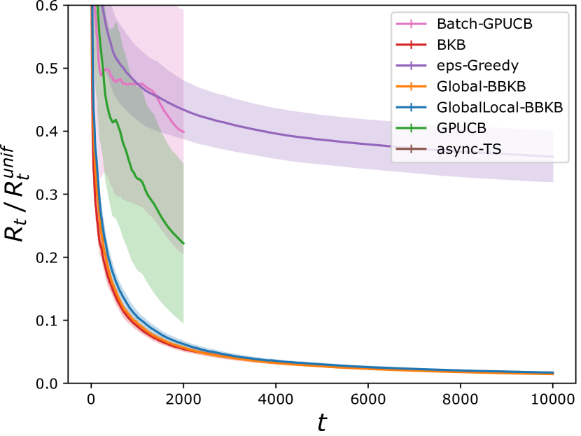
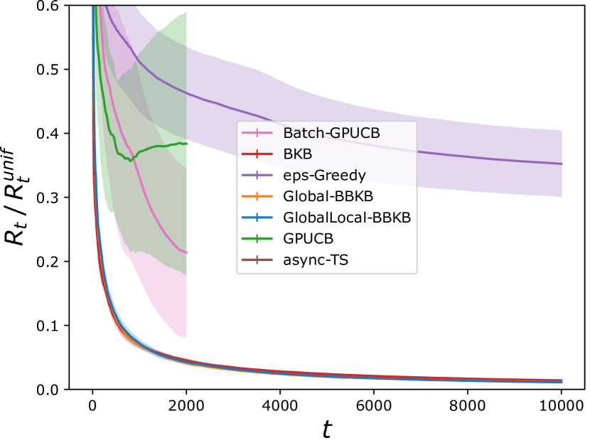
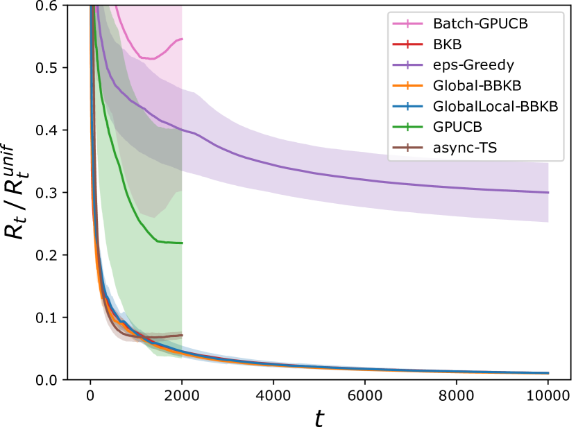
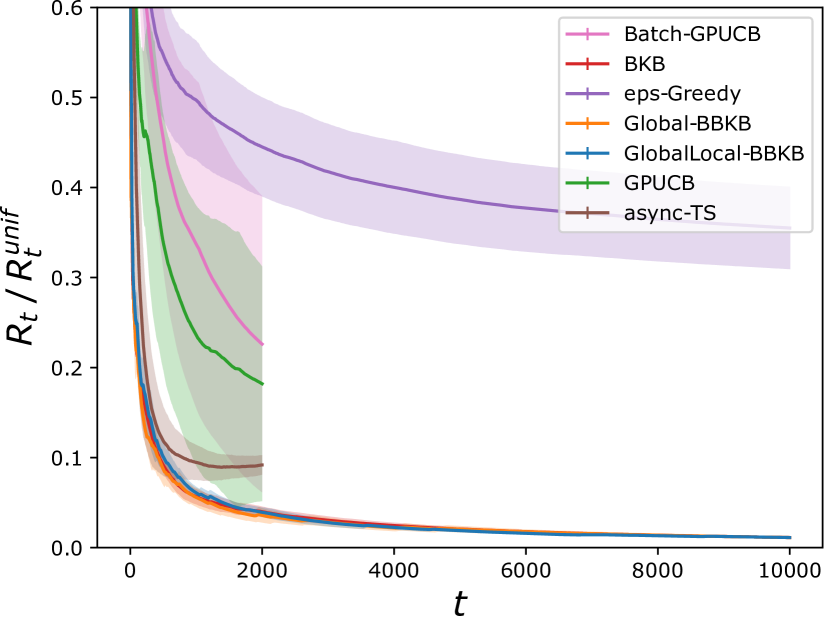
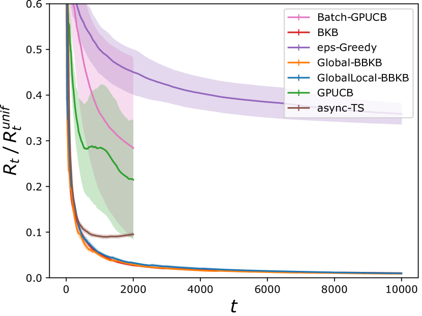
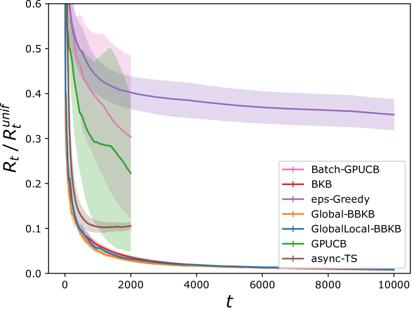
Fig. 5: Regret ratio for the Abalone dataset, with Gaussian kernel with, from left to right and from top to bottom, badwidths equal to $5,7.5,10,12.5,15,17.5$

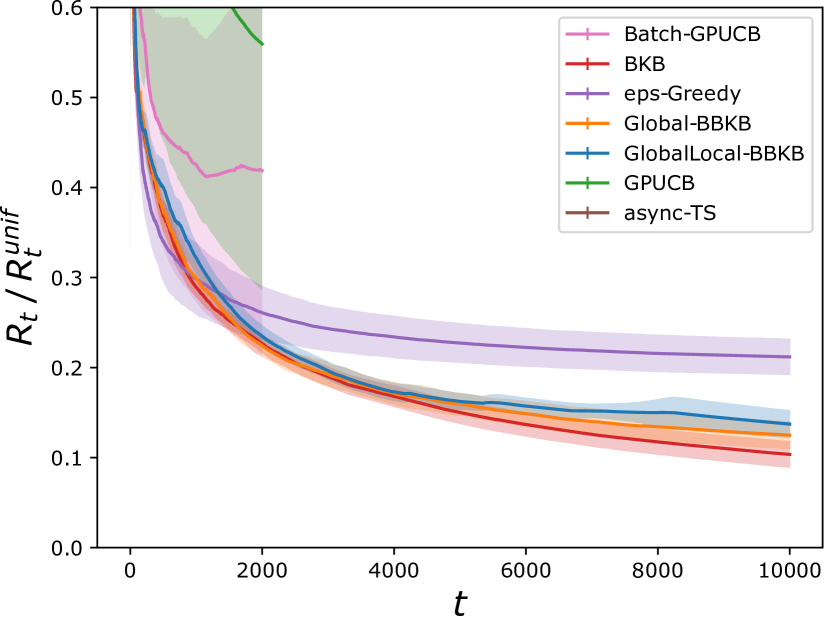
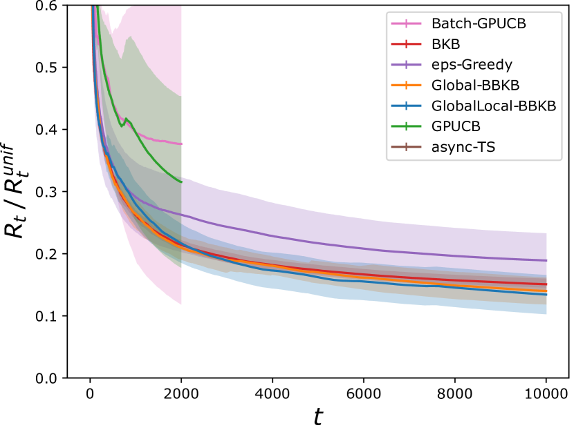
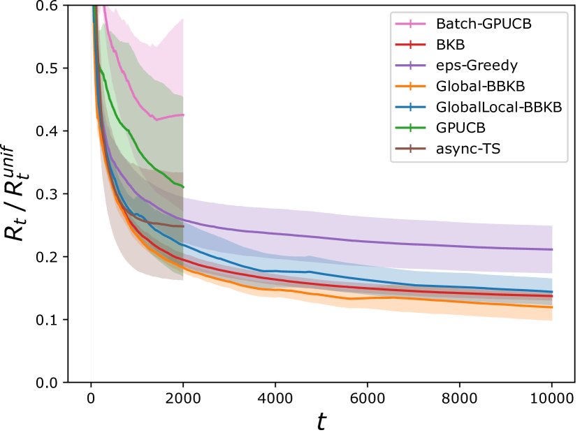
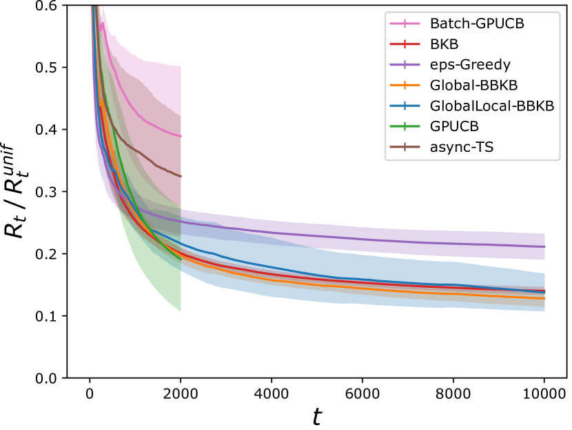
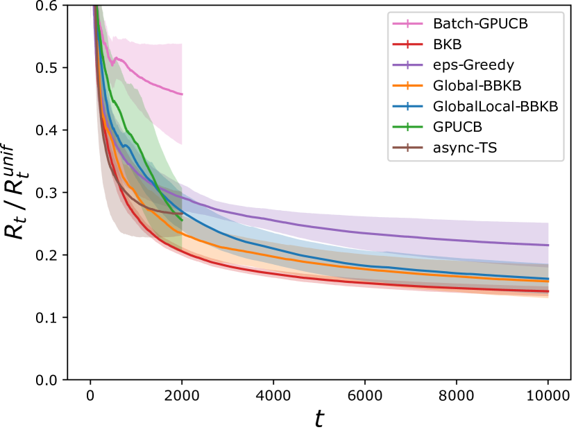
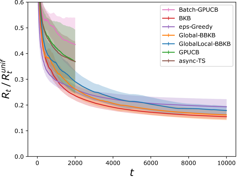
Fig. 6: Regret ratio for the Cadata dataset, with Gaussian kernel with, from left to right and from top to bottom, badwidths equal to $5,7.5,10,12.5,15,17.5$

D.2 NAS-bench-101

We use a subset of NAS-bench-101, generated using the following procedure. The whole NAS-bench-101 dataset contains architecture with 1 to 5 inner nodes, and up to 3 different kind of nodes ($3x3$ and $1x1$ convolutions, and $3x3$ max-pooling). We restrict ourselves to only architectures with exactly 4 inner nodes, and restrict the node type to only $3x3$ convolutions or max-pooling.

This kind of architectures are represented as the concatenation of a 15-dimensional vector, which is the flattened representation of the upper half of the network’s adjacency matrix, and a 4-dimensional $\{0,1\}$ vector indicating whether each inner node is a convolution ($1$) or a max-pooling ($0$).

For the 15-dimensional vector, we remove the first and last feature (corresponding to connection from the input and to the output) as they are present in all architecture and result in a constant feature of 1 that is not influential for learning. Finally, for each of these two halves of the representation, we renormalize each half separately to have at most unit norm and then concatenate the two halves. This strategy makes it so that each quantity (i.e., similarity in adjacency or similarity in node type) carries roughly the same weight.

Both Global-BBKB and GlobalLocal-BBKB uses a Gaussian kernel with $\sigma=125$ for the experiments with initialization, and $\sigma=100$ for the experiment without initialization. And as for the other experiments $F=1,\delta=1/T,\overline{q}=2$. The implementation of Reg-evolution is taken from https://github.com/automl/nas_benchmarks, and we leave the hyper-parameters to the default values chosen by the authors in Ying et al. [2019] as optimal. For completeness we report in Figure 7 regret ratio, batch size, time and time with training of the experiments on NAS-bench-101 without initialization.

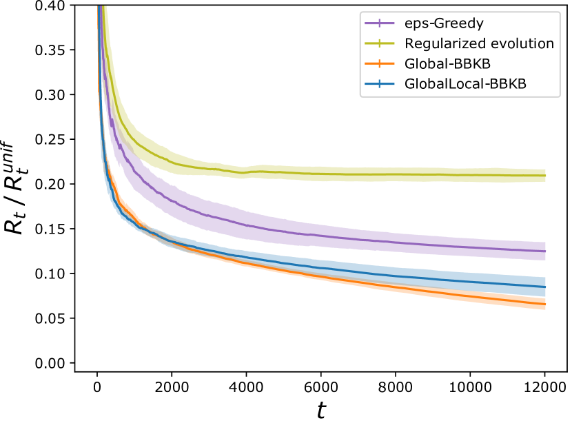
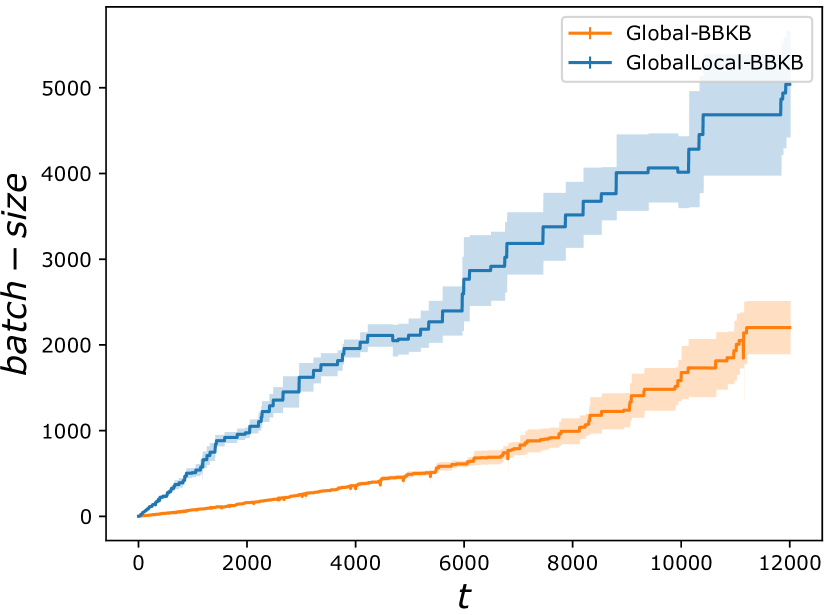
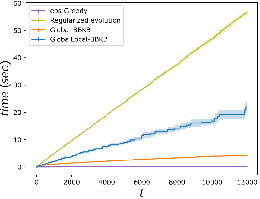
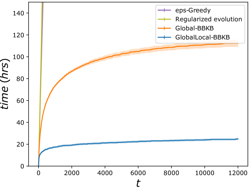
Fig. 7: From left to right and from top to bottom: regret ratio, batch-size, time without experimental costs and total runtime on the NAS-bench-101 dataset, with Gaussian kernel with bandwith $100$

References

- Abbasi-Yadkori et al. [2011] Abbasi-Yadkori, Y., Pál, D., and Szepesvári, C. Improved algorithms for linear stochastic bandits. In Advances in Neural Information Processing Systems, pp. 2312–2320, 2011.
- Alaoui & Mahoney [2015] Alaoui, A. E. and Mahoney, M. W. Fast randomized kernel methods with statistical guarantees. In Neural Information Processing Systems, 2015.
- Calandriello et al. [2017a] Calandriello, D., Lazaric, A., and Valko, M. Second-order kernel online convex optimization with adaptive sketching. In International Conference on Machine Learning, 2017a.
- Calandriello et al. [2017b] Calandriello, D., Lazaric, A., and Valko, M. Distributed adaptive sampling for kernel matrix approximation. In AISTATS, 2017b.
- Calandriello et al. [2019] Calandriello, D., Carratino, L., Lazaric, A., Valko, M., and Rosasco, L. Gaussian process optimization with adaptive sketching: Scalable and no regret. In Conference on Learning Theory, 2019.
- Chevalier & Ginsbourger [2013] Chevalier, C. and Ginsbourger, D. Fast computation of the multi-points expected improvement with applications in batch selection. In International Conference on Learning and Intelligent Optimization, pp. 59–69. Springer, 2013.
- Chowdhury & Gopalan [2017] Chowdhury, S. R. and Gopalan, A. On kernelized multi-armed bandits. In International Conference on Machine Learning, pp. 844–853, 2017.
- Contal et al. [2013] Contal, E., Buffoni, D., Robicquet, A., and Vayatis, N. Parallel Gaussian process optimization with upper confidence bound and pure exploration. In Joint European Conference on Machine Learning and Knowledge Discovery in Databases, pp. 225–240. Springer, 2013.
- Daxberger & Low [2017] Daxberger, E. A. and Low, B. K. H. Distributed batch Gaussian process optimization. In Precup, D. and Teh, Y. W. (eds.), Proceedings of the 34th International Conference on Machine Learning, volume 70 of Proceedings of Machine Learning Research, pp. 951–960, International Convention Centre, Sydney, Australia, 06–11 Aug 2017. PMLR.
- Desautels et al. [2014] Desautels, T., Krause, A., and Burdick, J. W. Parallelizing exploration-exploitation tradeoffs in Gaussian process bandit optimization. The Journal of Machine Learning Research, 15(1):3873–3923, 2014.
- Hennig & Schuler [2012] Hennig, P. and Schuler, C. J. Entropy Search for Information-Efficient Global Optimization. Journal of Machine Learning Research, 13:1809–1837, 2012.
- Huggins et al. [2019] Huggins, J. H., Campbell, T., Kasprzak, M., and Broderick, T. Scalable gaussian process inference with finite-data mean and variance guarantees. International Conference on Artificial Intelligence and Statistics, 2019.
- Kandasamy et al. [2018] Kandasamy, K., Krishnamurthy, A., Schneider, J., and Póczos, B. Parallelised bayesian optimisation via thompson sampling. In International Conference on Artificial Intelligence and Statistics, pp. 133–142, 2018.
- Kathuria et al. [2016] Kathuria, T., Deshpande, A., and Kohli, P. Batched gaussian process bandit optimization via determinantal point processes. In Advances in Neural Information Processing Systems, pp. 4206–4214, 2016.
- Mutny & Krause [2018] Mutny, M. and Krause, A. Efficient High Dimensional Bayesian Optimization with Additivity and Quadrature Fourier Features. In Bengio, S., Wallach, H., Larochelle, H., Grauman, K., Cesa-Bianchi, N., and Garnett, R. (eds.), Advances in Neural Information Processing Systems 31, pp. 9019–9030. Curran Associates, Inc., 2018.
- Quinonero-Candela et al. [2007] Quinonero-Candela, J., Rasmussen, C. E., and Williams, C. K. Approximation methods for gaussian process regression. Large-scale kernel machines, pp. 203–224, 2007.
- Rasmussen & Williams [2006] Rasmussen, C. E. and Williams, C. K. I. Gaussian processes for machine learning. Adaptive computation and machine learning. MIT Press, Cambridge, Mass, 2006. ISBN 978-0-262-18253-9. OCLC: ocm61285753.
- Real et al. [2019] Real, E., Aggarwal, A., Huang, Y., and Le, Q. V. Regularized evolution for image classifier architecture search. In Proceedings of the aaai conference on artificial intelligence, volume 33, pp. 4780–4789, 2019.
- Rudi et al. [2018] Rudi, A., Calandriello, D., Carratino, L., and Rosasco, L. On fast leverage score sampling and optimal learning. In Advances in Neural Information Processing Systems 31, pp. 5672–5682. 2018.
- Seeger et al. [2003] Seeger, M., Williams, C., and Lawrence, N. Fast forward selection to speed up sparse gaussian process regression. In Artificial Intelligence and Statistics 9, number EPFL-CONF-161318, 2003.
- Shah & Ghahramani [2015] Shah, A. and Ghahramani, Z. Parallel predictive entropy search for batch global optimization of expensive objective functions. In Advances in Neural Information Processing Systems, pp. 3330–3338, 2015.
- Srinivas et al. [2010] Srinivas, N., Krause, A., Seeger, M., and Kakade, S. M. Gaussian process optimization in the bandit setting: No regret and experimental design. In International Conference on Machine Learning, pp. 1015–1022, 2010.
- Valko et al. [2013] Valko, M., Korda, N., Munos, R., Flaounas, I., and Cristianini, N. Finite-time analysis of kernelised contextual bandits. In Proceedings of the Twenty-Ninth Conference on Uncertainty in Artificial Intelligence, pp. 654–663. AUAI Press, 2013.
- Wang et al. [2018] Wang, Z., Gehring, C., Kohli, P., and Jegelka, S. Batched large-scale bayesian optimization in high-dimensional spaces. In International Conference on Artificial Intelligence and Statistics, pp. 745–754, 2018.
- Wilson & Nickisch [2015] Wilson, A. and Nickisch, H. Kernel interpolation for scalable structured gaussian processes (kiss-gp). In International Conference on Machine Learning, pp. 1775–1784, 2015.
- Woodruff et al. [2014] Woodruff, D. P. et al. Sketching as a tool for numerical linear algebra. Foundations and Trends® in Theoretical Computer Science, 10(1–2):1–157, 2014.
- Ying et al. [2019] Ying, C., Klein, A., Real, E., Christiansen, E., Murphy, K., and Hutter, F. Nas-bench-101: Towards reproducible neural architecture search. arXiv preprint arXiv:1902.09635, 2019.