On mix-norms and the rate of
decay of correlations

Abstract.

Two quantitative notions of mixing are the decay of correlations and the decay of a mix-norm — a negative Sobolev norm — and the intensity of mixing can be measured by the rates of decay of these quantities. From duality, correlations are uniformly dominated by a mix-norm; but can they decay asymptotically faster than the mix-norm? We answer this question by constructing an observable with correlation that comes arbitrarily close to achieving the decay rate of the mix-norm. Therefore the mix-norm is the sharpest rate of decay of correlations in both the uniform sense and the asymptotic sense. Moreover, there exists an observable with correlation that decays at the same rate as the mix-norm if and only if the rate of decay of the mix-norm is achieved by its projection onto low-frequency Fourier modes. In this case, the function being mixed is called $q$-recurrent; otherwise it is $q$-transient. We use this classification to study several examples and raise questions for future investigations.

1. Introduction

Consider a spatially-periodic mean-zero function $f^{t}(\bm{x})=f(t,\bm{x})$ bounded uniformly in $L^{2}(\mathbb{T}^{d})$ for all $t>0$. For example, $f(t,\bm{x})$ might be a solution to the advection-diffusion equation

$$\frac{\partial f}{\partial t}+\bm{u}\cdot\nabla f=D\Delta f,$$ (1.1)

with $f^{0}\in L^{2}(\mathbb{T}^{d})$ and smooth divergence-free velocity field $\bm{u}(t,\bm{x})$. We may also consider $D=0$ in Eq. 1.1, in which case it is the transport equation. Another example, in the context of dynamical systems, is when an initial condition $f^{0}\in L^{2}$ is transported by an area-preserving map $M$ via the transfer operator $f^{n+1}=f^{n}\circ M^{-1}$.

Decay of the correlation function $C_{t}(g)=\mathopen{}\mathclose{{}\left|\mathopen{}\mathclose{{}\left\langle f^{t}\,,\,g}\right\rangle}\right|$ as $t\to\infty$ for observables $g$ in $L^{2}(\mathbb{T}^{d})$ corresponds to mixing of $f^{t}$ as $t\to\infty$ [32]. Mathew et al. [25] introduced the $H^{-1/2}$ norm as another criterion to quantify mixing, and Lin et al. [19] extended this to any negative Sobolev (e.g., $H^{-q}$) norm and showed that correlations decay to zero if and only if any such “mix-norm” decays to zero. That is,

$$\lim_{t\to\infty}\mathopen{}\mathclose{{}\left\langle f^{t}\,,\,g}\right\rangle=0\quad\forall g\in L^{2}\iff\lim_{t\to\infty}\mathopen{}\mathclose{{}\left\lVert f^{t}}\right\rVert_{H^{-q}}=0\text{, for any }q>0.$$

Mix-norms are well-suited to quantification of mixing efficiencies [9, 18, 31, 33, 34, 35, 23, 36], to lower bounds on the rate of mixing in general [15, 21, 22], and to analyzing mixing [24, 26, 27, 37]. Moreover, such negative Sobolev spaces provide a natural setting for a discussion of enhanced dissipation and relaxation [1, 3, 6, 7, 8, 12, 16, 17]. Mathew et al. [25] introduced the mix-norm in the context of spatial averages over strips, and made the connection to weak convergence (see also [39]).

While mix-norms are well-adapted to the PDE context, correlations and weak convergence are more commonly studied in the context of ergodic theory. A central question, then, is the quantitative relationship between decay rate of correlations and and decay of mix-norms. This is the central focus of this paper where we will work in a setting where the evolution of a function $f^{t}(\bm{x})$ is given, arising from the continuous-time solution of a PDE or in discrete times from an iterated map.

When studying a collection of functions converging to zero at $t\rightarrow\infty$, such as $\mathopen{}\mathclose{{}\left|\mathopen{}\mathclose{{}\left\langle f^{t}\,,\,g}\right\rangle}\right|$ for $g\in X$ where $X\subset L^{2}$ is some Banach space, there are several reasonable ways to define a rate of decay:

1. We can consider a uniform upper bound [2, 5, 10, 20, 30].

2. We can say that each function is $\mathcal{O}\mathopen{}\mathclose{{}\left(\varrho}\right)$ where $\varrho(t)$ is some rate function [38]. This lifts the tail of the rate function by multiplying by a constant that depends on $g\in X$.

3. We can instead lift the tail of the rate function by translation and say that each function is bounded above by a translation of some rate function [11].

We summarize as follows (for concreteness, fix some $q>0$ and consider $X=H^{q}(\mathbb{T}^{d})$):

1. Correlations decay at the uniform rate $r(t)$ for $g\in H^{q}$ if

   $$\mathopen{}\mathclose{{}\left|\mathopen{}\mathclose{{}\left\langle f^{t}\,,\,g}\right\rangle}\right|\leq r(t)\mathopen{}\mathclose{{}\left\lVert g}\right\rVert_{H^{q}}~{}\forall g\in H^{q}\,.$$ (1.2)

2. Correlations decay at the asymptotic rate $\varrho(t)$ for $g\in H^{q}$ if

   $$\mathopen{}\mathclose{{}\left|\mathopen{}\mathclose{{}\left\langle f^{t}\,,\,g}\right\rangle}\right|=\mathcal{O}\mathopen{}\mathclose{{}\left(\varrho}\right)\text{, for each }g\in H^{q}\,.$$ (1.3)

3. Correlations decay at the translational rate $\lambda(t)$ for $g\in H^{q}$ if for each $g\in H^{q}$ there exists $\tau\in\mathds{R}$ such that for all $t>\tau$ we have

   $$\mathopen{}\mathclose{{}\left|\mathopen{}\mathclose{{}\left\langle f^{t}\,,\,g}\right\rangle}\right|\leq\lambda(t-\tau)\mathopen{}\mathclose{{}\left\lVert g}\right\rVert_{H^{q}}\,.$$ (1.4)

Duality implies that the smallest uniform rate is the mix-norm $\mathopen{}\mathclose{{}\left\lVert f^{t}}\right\rVert_{H^{-q}}.$ Since any uniform rate trivially satisfies the definitions of asymptotic rate and translational rate, the question is whether there is a $\varrho$ (or $\lambda$) that decays faster than $\mathopen{}\mathclose{{}\left\lVert f^{t}}\right\rVert_{H^{-q}}$. We answer this question by showing that we cannot have $\varrho=o\mathopen{}\mathclose{{}\left(\mathopen{}\mathclose{{}\left\lVert f^{t}}\right\rVert_{H^{-q}}}\right)$. Similarly, given the additional assumption that $\limsup_{t\to\infty}\lambda(t-\tau)/\lambda(t)$ is finite, we cannot have $\lambda=o\mathopen{}\mathclose{{}\left(\mathopen{}\mathclose{{}\left\lVert f^{t}}\right\rVert_{H^{-q}}}\right)$. We do this by constructing an observable $g\in H^{q}$ such that $\lvert\mathopen{}\mathclose{{}\left\langle f^{t}\,,\,g}\right\rangle\rvert$ decays arbitrarily closely to the mix-norm. Namely, for any positive $h(t)=o\mathopen{}\mathclose{{}\left(\mathopen{}\mathclose{{}\left\lVert f^{t}}\right\rVert_{H^{-q}}}\right)$ there is a $g\in H^{q}$ such that $\lvert\mathopen{}\mathclose{{}\left\langle f^{t}\,,\,g}\right\rangle\rvert$ is Big-O but not Little-O of $h$.

Note that this is not the same as asymptotic equivalence because the correlation may be much smaller than $h$ at certain times. Moreover, we may take $h=\mathopen{}\mathclose{{}\left\lVert f^{t}}\right\rVert_{H^{-q}}$ above if and only if there is a finite set $I$ of Fourier modes where the $H^{-q}$ norm of the projection $P_{I}f^{t}$ of $f^{t}$ onto the modes $I$ is Big-O but not Little-O of $\mathopen{}\mathclose{{}\left\lVert f^{t}}\right\rVert_{H^{-q}}$. In this case, we refer to $f^{t}$ as $q$-recurrent (otherwise it is $q$-transient) and the decay of the mix-norm is characterized by $P_{I}f^{t}$.

In Section 2 we introduce the key definitions and main theorems. Section 3 contains examples, and Sections 4 and 5 contains the full proofs to the theorems.

2. Overview

Throughout, it will be more convenient to work with the homogeneous Sobolev spaces $\dot{H}^{\alpha}$ for $\alpha\in\mathds{R}$. Since the torus $\mathbb{T}^{d}$ is a compact manifold, Poincaré’s inequality applies [14] so that the $H^{\alpha}$ norm and $\dot{H}^{\alpha}$ norm are equivalent for mean-zero functions. For $\alpha>0$, the $\dot{H}^{-\alpha}$ norm is typically defined via the duality equation

$$\mathopen{}\mathclose{{}\left\lVert f}\right\rVert_{\dot{H}^{-\alpha}}=\sup\limits_{\begin{subarray}{c}g\in\dot{H}^{\alpha}\end{subarray}}\frac{\lvert\mathopen{}\mathclose{{}\left\langle f\,,\,g}\right\rangle\rvert}{\mathopen{}\mathclose{{}\left\lVert g}\right\rVert_{\dot{H}^{\alpha}}}.$$

However, there is an equivalent definition [13] for all $\alpha\in\mathbb{R}$. Let $f_{{\bm{k}}}=\int_{\mathbb{T}^{d}}f(\bm{x})\,\mathrm{e}^{-2\pi i\bm{x}\cdot{\bm{k}}}~{}d\bm{x}$ denote the Fourier coefficients of $f(\bm{x})$. Then

$$\mathopen{}\mathclose{{}\left\lVert f}\right\rVert_{\dot{H}^{\alpha}}=\mathopen{}\mathclose{{}\left(\sum_{{\bm{k}}\neq\bm{0}}k^{2\alpha}\,|f_{{\bm{k}}}|^{2}}\right)^{1/2}$$

where $k^{2}=|{\bm{k}}|^{2}=|k_{1}|^{2}+\dots+|k_{d}|^{2}$. We will typically omit the ${\bm{k}}\neq 0$ on the sum since $f_{\bm{0}}=0$ for mean-zero functions.

Similarly, correlations have a simple expression. Since the trigonometric functions $\{\mathrm{e}^{2\pi i\bm{x}\cdot{\bm{k}}}\}$ provide an orthonormal basis for $L^{2}(\mathbb{T}^{d})$, the Fourier transform is a unitary map to $\ell^{2}(\mathbb{Z}^{d})$. Therefore the Fourier transform preserves the inner product [13] and we have Plancherel’s Theorem:

$$\mathopen{}\mathclose{{}\left\langle f\,,\,g}\right\rangle=\sum_{{\bm{k}}}f_{\bm{k}}~{}\bar{g}_{\bm{k}}\quad\forall f,g\in L^{2}(\mathbb{T}^{d}).$$

For time-dependent $f^{t}(\bm{x})$, the duality equation implies $\mathopen{}\mathclose{{}\left|\mathopen{}\mathclose{{}\left\langle f^{t}\,,\,g}\right\rangle}\right|\leq\mathopen{}\mathclose{{}\left\lVert f^{t}}\right\rVert_{\dot{H}^{-q}}\mathopen{}\mathclose{{}\left\lVert g}\right\rVert_{\dot{H}^{q}}$ for all $t$. Moreover, fix $t=t_{0}$ and take $g$ with Fourier coefficients

$$g_{\bm{k}}=f_{\bm{k}}^{t_{0}}\,k^{-2q}\mathopen{}\mathclose{{}\left\lVert f^{t_{0}}}\right\rVert_{\dot{H}^{-q}}^{-1}.$$ (2.1)

Then $\mathopen{}\mathclose{{}\left\lVert g}\right\rVert_{\dot{H}^{q}}=1$ and Plancherel’s Theorem gives $\mathopen{}\mathclose{{}\left\langle f^{t_{0}}\,,\,g}\right\rangle=\mathopen{}\mathclose{{}\left\lVert f^{t_{0}}}\right\rVert_{\dot{H}^{-q}}$. The correlation achieves the mix-norm at the time $t_{0}$. Since $t_{0}$ is arbitrary, we see that $\mathopen{}\mathclose{{}\left\lVert f^{t}}\right\rVert_{\dot{H}^{-q}}$ is the envelope of the set of functions $\mathopen{}\mathclose{{}\left|\mathopen{}\mathclose{{}\left\langle f^{t}\,,\,g}\right\rangle}\right|$ with $\mathopen{}\mathclose{{}\left\lVert g}\right\rVert_{\dot{H}^{q}}=1$, as in Fig. 1.

Figure 1. Plotted above are the mix-norm and correlations with different choices of $g$, demonstrating that the mix-norm is the envelope over $\mathopen{}\mathclose{{}\left|\mathopen{}\mathclose{{}\left\langle f^{t}\,,\,g}\right\rangle}\right|$ with $\mathopen{}\mathclose{{}\left\lVert g}\right\rVert_{\dot{H}^{q}}=1$.

Remark.

We assume in Eq. 2.1 that $\mathopen{}\mathclose{{}\left\lVert f^{t_{0}}}\right\rVert_{\dot{H}^{-q}}>0$. The case $\mathopen{}\mathclose{{}\left\lVert f^{t_{0}}}\right\rVert_{\dot{H}^{-q}}=0$ is degenerate in the context of the advection-diffusion equation and dynamical systems. In those settings, if the mix-norm is zero at any finite time it will remain zero for future times. Hence we subsequently assume that $\mathopen{}\mathclose{{}\left\lVert f^{t}}\right\rVert_{\dot{H}^{-q}}>0$ for all $t>0$ to simplify the presentation of our results.

Using only duality, the most that can be said about the relationship between the rate of decay of a correlation and the rate of decay of the mix-norm is that

$$\mathopen{}\mathclose{{}\left|\mathopen{}\mathclose{{}\left\langle f^{t}\,,\,g}\right\rangle}\right|=\mathcal{O}\mathopen{}\mathclose{{}\left(\mathopen{}\mathclose{{}\left\lVert f^{t}}\right\rVert_{\dot{H}^{-q}}}\right)\text{ for each }g\in\dot{H}^{q}.$$

However, each correlation could decay strictly faster than the mix-norm as illustrated in Fig. 1. We are then led to ask if such a situation is possible.

When is $\mathopen{}\mathclose{{}\left|\mathopen{}\mathclose{{}\left\langle f^{t}\,,\,g}\right\rangle}\right|=o\mathopen{}\mathclose{{}\left(\mathopen{}\mathclose{{}\left\lVert f^{t}}\right\rVert_{\dot{H}^{-q}}}\right)$ for each $g\in\dot{H}^{q}\,$? To answer this question, we must construct functions $g\in\dot{H}^{q}$ such that the correlations $\mathopen{}\mathclose{{}\left|\mathopen{}\mathclose{{}\left\langle f^{t}\,,\,g}\right\rangle}\right|$ decay as slowly as possible. To do this, we first classify $f^{t}$ as either $q$-recurrent or $q$-transient as follows.

For a set $I\subset\mathds{Z}^{d}$ let

$$P_{I}f^{t}=\sum_{{\bm{k}}\in I}f^{t}_{\bm{k}}\,\mathrm{e}^{2\pi i\bm{x}\cdot{\bm{k}}}$$

denote the projection of $f^{t}$ onto the Fourier modes ${\bm{k}}\in I$. Then

$$\mathopen{}\mathclose{{}\left\lVert P_{I}f^{t}}\right\rVert_{\dot{H}^{-q}}^{2}=\sum\limits_{{\bm{k}}\in I}k^{-2q}\,|f_{\bm{k}}^{t}|^{2}$$

measures the amount of mix-norm supported on $I$. We often refer to this as the Fourier energy contained in $I$. This notion of energy is $q$-dependent, though the $q$ will usually be clear from the context.

Definition 1.

We say $f^{t}$ is $q$-recurrent if there exists a finite set $I\subset\mathds{Z}^{d}$ such that

$$\limsup_{t\to\infty}\frac{\mathopen{}\mathclose{{}\left\lVert P_{I}f^{t}}\right\rVert_{\dot{H}^{-q}}}{\mathopen{}\mathclose{{}\left\lVert f^{t}}\right\rVert_{\dot{H}^{-q}}}>0.$$ (2.2)

Functions that are not $q$-recurrent will be called $q$-transient.

Remark.

We emphasize that $q$-recurrence is a property of $f^{t}$ which encompasses both the stirring action and the initial condition coupled together. To clarify, in the context of the advection-diffusion equation (1.1), $q$-recurrence is a property of a particular realization of $\bm{u}$ and $f^{0}$ taken together – it is not just a property of the vector field $\bm{u}$. Moreover, a given $f^{t}$ may be $q$-recurrent for some (larger) values of $q$ and $q$-transient for other (smaller) $q$.

From inequality (2.2) and the trivial bound $\mathopen{}\mathclose{{}\left\lVert P_{I}f^{t}}\right\rVert_{\dot{H}^{-q}}\leq\mathopen{}\mathclose{{}\left\lVert f^{t}}\right\rVert_{\dot{H}^{-q}}$ we see that $\mathopen{}\mathclose{{}\left\lVert P_{I}f^{t}}\right\rVert_{\dot{H}^{-q}}$ is Big-O but not Little-O of $\mathopen{}\mathclose{{}\left\lVert f^{t}}\right\rVert_{\dot{H}^{-q}}$. Unpacking the definition of limit supremum offers another interpretation: there exists $\delta>0$ and a sequence $t_{m}\to\infty$ where

$$\mathopen{}\mathclose{{}\left\lVert P_{I}f^{t_{m}}}\right\rVert_{\dot{H}^{-q}}\geq\delta\mathopen{}\mathclose{{}\left\lVert f^{t_{m}}}\right\rVert_{\dot{H}^{-q}}.$$ (2.3)

This means that there is at least a $\delta$ fraction of the mix-norm supported on $I$ at arbitrarily large times. As time progresses the Fourier energy could move off of $I$, but we can always find a future time $t_{m+1}$ where a proportion $\delta$ of the mix-norm is again on $I$. In other words, some Fourier energy always returns to populate the spatial scales in $I$. In this case, test functions $g$ with coefficients for ${\bm{k}}\in I$ similar to that in Eq. 2.1 will match well with $f^{t}$ at times $t_{m}$ (after possibly taking a subsequence) so that in Section 4 we can prove the following theorem, a central result of our paper.

Theorem 1.

Let $f^{t}$ be a mean-zero function in $L^{2}(\mathbb{T}^{d})$ with $\mathopen{}\mathclose{{}\left\lVert f^{t}}\right\rVert_{\dot{H}^{-q}}>0$ for all $t>0$. Then $f^{t}$ is $q$-recurrent if and only if there is a function $g\in\dot{H}^{q}$ such that

$$\limsup_{t\to\infty}\frac{\mathopen{}\mathclose{{}\left|\mathopen{}\mathclose{{}\left\langle f^{t}\,,\,g}\right\rangle}\right|}{\mathopen{}\mathclose{{}\left\lVert f^{t}}\right\rVert_{\dot{H}^{-q}}}>0.$$

Equivalently, there is a function $g\in\dot{H}^{q}$, a constant $c>0$, and a sequence $t_{m}\to\infty$ where

$$\mathopen{}\mathclose{{}\left|\mathopen{}\mathclose{{}\left\langle f^{t_{m}}\,,\,g}\right\rangle}\right|\geq c\,\mathopen{}\mathclose{{}\left\lVert f^{t_{m}}}\right\rVert_{\dot{H}^{-q}}.$$ (2.4)

Figure 2. There exists $g\in\dot{H}^{q}$ where $\mathopen{}\mathclose{{}\left|\mathopen{}\mathclose{{}\left\langle f^{t}\,,\,g}\right\rangle}\right|$ does not decay faster than $c\mathopen{}\mathclose{{}\left\lVert f^{t}}\right\rVert_{\dot{H}^{-q}}$.

Remark.

As demonstrated in Fig. 2, it is possible that $\mathopen{}\mathclose{{}\left|\mathopen{}\mathclose{{}\left\langle f^{t}\,,\,g}\right\rangle}\right|$ is small at times $t\neq t_{m}$ and so we do not show asymptotic equivalence. We interpret our result as demonstrating that the correlation does not decay asymptotically faster than the mix-norm in the sense that $\mathopen{}\mathclose{{}\left|\mathopen{}\mathclose{{}\left\langle f^{t}\,,\,g}\right\rangle}\right|$ is Big-O but not Little-O of $\mathopen{}\mathclose{{}\left\lVert f^{t}}\right\rVert_{\dot{H}^{-q}}$. From this theorem, the answer to our previously posed question ‘when is $\mathopen{}\mathclose{{}\left|\mathopen{}\mathclose{{}\left\langle f^{t}\,,\,g}\right\rangle}\right|=o\mathopen{}\mathclose{{}\left(\mathopen{}\mathclose{{}\left\lVert f^{t}}\right\rVert_{\dot{H}^{-q}}}\right)$ for each $g\in\dot{H}^{q}\,$?’ is exactly when $f^{t}$ is $q$-transient.

This naturally prompts us to ask if $f^{t}$ is $q$-transient and we carefully choose $g\in\dot{H}^{q}$, how slowly can we make $\mathopen{}\mathclose{{}\left|\mathopen{}\mathclose{{}\left\langle f^{t}\,,\,g}\right\rangle}\right|$ decay? The following theorem answers this question.

Theorem 2.

Let $f^{t}$ be a mean-zero function in $L^{2}(\mathbb{T}^{d})$ with $\mathopen{}\mathclose{{}\left\lVert f^{t}}\right\rVert_{\dot{H}^{-q}}>0$ for all $t>0$. For any positive function $h(t)$ such that $h(t)=o\mathopen{}\mathclose{{}\left(\mathopen{}\mathclose{{}\left\lVert f^{t}}\right\rVert_{\dot{H}^{-q}}}\right)$, there is a function $g\in\dot{H}^{q}$ such that

$$\limsup_{t\to\infty}\frac{\mathopen{}\mathclose{{}\left|\mathopen{}\mathclose{{}\left\langle f^{t}\,,\,g}\right\rangle}\right|}{h(t)}>0.$$

Remark.

Theorems 1 and 2 do not require $f^{t}$ to be bounded uniformly in $L^{2}(\mathbb{T}^{d})$ in time, nor for the mix-norm to decay to zero. Additionally, Theorem 2 is valid whether $f^{t}$ is $q$-recurrent or $q$-transient.

The proof of Theorem 2 is deferred until Section 5, but we present the idea behind the proof now. If $f^{t}$ is $q$-recurrent, then the proof is accomplished by a result similar to Theorem 1. For $q$-transient functions, the proof relies on the construction of sets $I_{m}$ and times $t_{m}$ satisfying certain properties, the first being that we want the finite disjoint sets $I_{m}\in\mathds{Z}^{d}$ to capture a large amount of the Fourier energy at time $t_{m}$. We can do this since $q$-transience ensures that we can wait for the next time $t_{m+1}$ for a proportion of the Fourier energy for moves off of $I_{m}$ and never comes back. Then by choosing the Fourier coefficients of $g$ on $I_{m}$ to agree with $f^{t}$ at time $t_{m}$, we can guarantee that $\mathopen{}\mathclose{{}\left|\mathopen{}\mathclose{{}\left\langle f^{t}\,,\,g}\right\rangle}\right|$ will be large at time $t_{m}$. Hence, the function $g$ in Theorem 2 which gives the slowly decaying $\mathopen{}\mathclose{{}\left|\mathopen{}\mathclose{{}\left\langle f^{t}\,,\,g}\right\rangle}\right|$ has Fourier coefficients

$$g_{\bm{k}}=\begin{cases}f_{\bm{k}}^{t_{m}}k^{-2q}\mathopen{}\mathclose{{}\left\lVert f^{t_{m}}}\right\rVert_{\dot{H}^{-q}}^{-2}\,h(t_{m}),&{\bm{k}}\in I_{m};\\ 0,&\text{otherwise};\\ \end{cases}$$ (2.5)

where $I_{m}$ are disjoint and $\mathopen{}\mathclose{{}\left\lVert P_{I_{m}}f^{t_{m}}}\right\rVert_{\dot{H}^{-q}}$ captures a nonzero proportion of $h(t_{m})$, similar to inequality (2.3). These coefficients are similar to those of Eq. 2.1 except with an extra factor of $h/\mathopen{}\mathclose{{}\left\lVert f}\right\rVert_{\dot{H}^{-q}}$. This factor is needed so that we can satisfy the second property we require from the sets $I_{m}$ and times $t_{m}$: by taking a subsequence, we can use the fact that $h(t)=o\mathopen{}\mathclose{{}\left(\mathopen{}\mathclose{{}\left\lVert f^{t}}\right\rVert_{\dot{H}^{-q}}}\right)$ to make the $g_{\bm{k}}$ decay fast enough as $k\to\infty$ to have $g\in\dot{H}^{q}$. Hence, although correlations may not achieve the decay rate of the mix-norm, they may achieve the decay rate of $h$.

These theorems allow us to show the result outlined in the introduction. The following corollary reveals it is not possible to find a $\varrho$ or $\lambda$ (under a given growth condition) that is Little-O of the mix-norm. We remark that the growth condition on $\lambda$ that $\limsup_{t\to\infty}\lambda(t-\tau)/\lambda(t)$ is finite is satisfied by power law and exponential functions but not by double exponential functions.

Corollary 1.

1. For any $\varrho$ satisfying Eq. 1.3, we have

   $$\limsup_{t\to\infty}\frac{\varrho(t)}{\mathopen{}\mathclose{{}\left\lVert f^{t}}\right\rVert_{H^{-q}}}>0\,.$$

2. For $\lambda$ satisfying Eq. 1.4 and $\limsup_{t\to\infty}\lambda(t-\tau)/\lambda(t)$ finite for any $\tau\in\mathds{R}$, we have

   $$\limsup_{t\to\infty}\frac{\lambda(t)}{\mathopen{}\mathclose{{}\left\lVert f^{t}}\right\rVert_{H^{-q}}}>0\,.$$

Proof of Corollary 1.

Seeking contradiction we suppose there is a $\varrho(t)$ satisfying Eq. 1.3 such that $\varrho(t)=o\mathopen{}\mathclose{{}\left(\mathopen{}\mathclose{{}\left\lVert f^{t}}\right\rVert_{\dot{H}^{-q}}}\right)$. Choosing $h(t)=\sqrt{\varrho(t)\mathopen{}\mathclose{{}\left\lVert f^{t}}\right\rVert_{\dot{H}^{-q}}}$, the geometric mean of $\varrho$ and the mix-norm, we see

$$\limsup_{t\to\infty}\frac{h}{\mathopen{}\mathclose{{}\left\lVert f^{t}}\right\rVert_{\dot{H}^{-q}}}=\limsup_{t\to\infty}\sqrt{\frac{\varrho}{\mathopen{}\mathclose{{}\left\lVert f^{t}}\right\rVert_{\dot{H}^{-q}}}}=0\,.$$ (2.6)

Then Theorem 2 assures there is a $g\in\dot{H}^{q}$ with

$$\limsup_{t\to\infty}\frac{\mathopen{}\mathclose{{}\left|\mathopen{}\mathclose{{}\left\langle f^{t}\,,\,g}\right\rangle}\right|}{h}>0\,.$$

Then we have arrived at a contradiction:

$$\limsup_{t\to\infty}\frac{\mathopen{}\mathclose{{}\left|\mathopen{}\mathclose{{}\left\langle f^{t}\,,\,g}\right\rangle}\right|}{h}\leq\limsup_{t\to\infty}\frac{\mathopen{}\mathclose{{}\left|\mathopen{}\mathclose{{}\left\langle f^{t}\,,\,g}\right\rangle}\right|}{\varrho}\cdot\limsup_{t\to\infty}\frac{\varrho}{h}=0$$

since $\limsup_{t\to\infty}\mathopen{}\mathclose{{}\left|\mathopen{}\mathclose{{}\left\langle f^{t}\,,\,g}\right\rangle}\right|/\varrho$ is finite by Eq. 1.3 and $\limsup_{t\to\infty}\varrho/h=0$ as in Eq. 2.6.

A similar argument gives us the second half of the corollary. In this case choose $h(t)=\sqrt{\lambda(t)\mathopen{}\mathclose{{}\left\lVert f^{t}}\right\rVert_{\dot{H}^{-q}}}$ and apply Theorem 2 to produce a test function $g$ which comes with a $\tau$ from Eq. 1.4. Then we have another contradiction:

$$\limsup_{t\to\infty}\frac{\mathopen{}\mathclose{{}\left|\mathopen{}\mathclose{{}\left\langle f^{t}\,,\,g}\right\rangle}\right|}{h(t)}\leq\limsup_{t\to\infty}\frac{\mathopen{}\mathclose{{}\left|\mathopen{}\mathclose{{}\left\langle f^{t}\,,\,g}\right\rangle}\right|}{\lambda(t-\tau)}\cdot\limsup_{t\to\infty}\frac{\lambda(t-\tau)}{\lambda(t)}\cdot\limsup_{t\to\infty}\frac{\lambda(t)}{h(t)}=0$$

since $\limsup_{t\to\infty}\lambda(t-\tau)/\lambda(t)$ is finite by hypothesis. ∎

In Section 3 we present an example of a $q$-transient function and alter it to send energy down the spectrum less efficiently, resulting in $q$-recurrence for a range of $q$. We then include diffusion at every time step, demonstrating a transition to $q$-recurrence for all $q>0$. We include a numerical example and provide intuition about how to recognize when $f^{t}$ is $q$-recurrent. Finally, we prove the theorems in generality in Sections 4 and 5.

3. Examples

Example 1 (baker’s map and $q$-transience).

Figure 3. The baker’s map.

Let $B$ be the baker’s map, the area preserving transformation of the domain $[0,1]^{2}$ as pictured in Fig. 3. For the $y$-independent initial function $f^{0}(x,y)=2\cos\mathopen{}\mathclose{{}\left(2\pi x}\right)$, applying the baker’s map simply doubles the frequency in the $x$ direction. After $n$ applications of the baker’s map we have $f^{n}=f^{0}\circ B^{-n}$ $=2\cos\mathopen{}\mathclose{{}\left(2\pi~{}2^{n}x}\right)$. As a result, the Fourier coefficients have the simple expression

$$f_{{\bm{k}}}^{n}=\begin{cases}1&k_{1}=2^{n},k_{2}=0;\\ 0&\text{otherwise}.\end{cases}$$

This is a one dimensional action on Fourier coefficients $f^{n}_{k}=f^{n}_{k_{1},0}$ via an infinite dimensional matrix $A_{k\ell}$ as

$$f^{n+1}_{k}=\sum_{\ell}A_{k\ell}\,f^{n}_{\ell}$$ (3.1)

where

is populated by 1’s along a subdiagonal of slope $-2$ and 0’s everywhere else.

The entire mix-norm is supported on just one Fourier mode and given any finite set $I\in\mathds{Z}^{d}$, it is clear that, as $n$ increases, the Fourier energy will move off of $I$ and never return. Therefore $f^{n}$ is $q$-transient $\forall q>0$.

Example 2 (altered baker’s map action and $q$-recurrence).

We now alter the previous example so that the energy of $f^{n}$ is sent down the spectrum less effectively, the result being a $q$-recurrent function (if $q$ is large enough). This time, consider the action on the Fourier coefficients of $f^{n}(x)$ as in Eq. 3.1 via the infinite dimensional matrix

where $a,b>0$ are constants such that $a^{2}+b^{2}=1$.

Remark.

It is not evident that the current example is still a dynamical systems example. That is, we do not know that there is a map $T:[0,1]^{d}\to[0,1]^{d}$ so that $f^{n+1}=f^{n}\circ T$ and $f^{n+1}_{k}=\sum_{\ell}\widetilde{A}_{k\ell}\,f^{n}_{\ell}$ . Moreover, such a map might not be injective, surjective, or unique. For example, $B^{-1}$ from the previous example is not injective when thought of as a map on $[0,1]$, but it is when we allow it to move through another dimension ($d=2$). For the present example, taking $a,b=\sqrt{2}/2$, the initial function $f^{0}(x)=2\cos\mathopen{}\mathclose{{}\left(2\pi x}\right)$ is transformed to $f^{1}(x)=\sqrt{2}(a\cos\mathopen{}\mathclose{{}\left(2\pi x}\right)+b\cos\mathopen{}\mathclose{{}\left(4\pi x}\right))$ after one time step. Since the range of $f^{0}$ and $f^{1}$ are not the same set, any such $T$ cannot be surjective. Lastly, if $f^{n}$ is constant, then $T$ can be any map. These caveats notwithstanding, we consider the current example as a study of possible ways for energy to move down the spectrum and proceed with an analysis.

We show the coefficients of $f^{n}$ for initial function $f^{0}(x)=2\cos\mathopen{}\mathclose{{}\left(2\pi x}\right)$ in Table 1. Heuristically, the energy starts concentrated on the $k=1$ mode and subsequently splits between modes $k=1,2$ so that $L^{2}$ norm is preserved. After that the $k=1$ mode continues to donate a proportion $b$ of its energy to $k=2$ and the energy on $k=2$ is transported down the spectrum at the same rate as the baker’s map ($k=2^{n}$).

Notice that $f^{n}$ is mean-zero because it is the finite sum of cosine functions with full period. We can compute the $L^{2}$ norm and find $\mathopen{}\mathclose{{}\left\lVert f^{n}}\right\rVert_{L^{2}}=1~{}\forall n$. Hence $A_{k\ell}$ is a unitary map on $\ell^{2}$ by the polarization identity. Therefore $f^{n}$ is bounded uniformly in $L^{2}$ and so $f^{n}$ satisfies the hypothesis of the theorems in Section 2.

	$k=1$	2	3	4	5	6	7	8	…
$f^{0}_{k}$	1
$f^{1}_{k}$	$a$	$b$
$f^{2}_{k}$	$a^{2}$	$ab$		$b$
$f^{3}_{k}$	$a^{3}$	$a^{2}b$		$ab$				$b$
⋮

Table 1. Nonvanishing Fourier coefficients of $f^{n}$ defined by Eq. 3.1, for $f^{0}(x)=2\cos\mathopen{}\mathclose{{}\left({2\pi}x}\right)$.

Consider the contribution to the mix-norm from mode $k=1$

$$\mathcal{E}_{1}^{n}=\mathopen{}\mathclose{{}\left\lVert P_{k=1}f^{n}}\right\rVert_{\dot{H}^{-q}}^{2}=\sum\limits_{k=1}k^{-2q}|f_{k}^{n}|^{2}=|f_{1}^{n}|^{2}=a^{2n},$$

and compare it to the contributions from modes $k>1$ (a geometric sum):

$$\mathcal{E}_{k>1}^{n} =\mathopen{}\mathclose{{}\left\lVert P_{k>1}f^{n}}\right\rVert_{\dot{H}^{-q}}^{2}=\sum\limits_{k>1}k^{-2q}|f_{k}^{n}|^{2}$$

$$=\begin{cases}c_{q,a}\mathopen{}\mathclose{{}\left(a^{2n}-2^{-2qn}}\right),&\text{for }a\neq 2^{-q};\vspace{2mm}\\ b^{2}~{}a^{2n}n,&\text{for }a=2^{-q};\end{cases}$$

where

$$c_{q,a}=\frac{b^{2}}{a^{2}2^{2q}-1}.$$

For $a>2^{-q}$, we see that $\mathcal{E}_{1}^{n}\sim\mathcal{E}_{k>1}^{n}$ as $n\to\infty$ and the mode $k=1$ captures a non-zero proportion of the mix-norm for arbitrarily large $n$. Therefore $f^{n}$ is $q$-recurrent for $q>log_{2}(1/a)$.

For $a\leq 2^{-q}$, $\mathcal{E}_{1}^{n}=o\mathopen{}\mathclose{{}\left(\mathcal{E}_{k>1}^{n}}\right)$ so the mode $k=1$ does not capture a non-zero proportion of the mix-norm for arbitrarily large $n$. This suggests that $f^{n}$ is $q$-transient for $q\leq log_{2}(1/a)$. To prove $q$-transience, we need to show the same holds for an arbitrary finite set $I$. Take $I=\mathopen{}\mathclose{{}\left[0,2^{R}}\right]$ for some $R\in\mathds{N}$. For $n>R$,

$$\mathopen{}\mathclose{{}\left\lVert P_{I}f^{n}}\right\rVert_{\dot{H}^{-q}}^{2}=c_{R,q,a}~{}a^{2n}$$

where

$$c_{R,q,a}=\begin{cases}1+c_{q,a}\mathopen{}\mathclose{{}\left(1-a^{-2R}2^{-2qR}}\right),&\text{for }a\neq 2^{-q};\vspace{2mm}\\ 1+b^{2}R,&\text{for }a=2^{-q}\end{cases}$$

and we conclude that

$$\lim_{n\to\infty}\frac{\mathopen{}\mathclose{{}\left\lVert P_{I}f^{n}}\right\rVert^{2}_{\dot{H}^{-q}}}{\mathopen{}\mathclose{{}\left\lVert f^{n}}\right\rVert^{2}_{\dot{H}^{-q}}}=\begin{cases}c_{R,q,a}\mathopen{}\mathclose{{}\left(1+c_{q,a}}\right)^{-1},&\text{for }a>2^{-q};\\ 0,&\text{for }a\leq 2^{-q}.\end{cases}$$

Therefore $f^{n}$ is $q$-transient for $q\leq log_{2}(1/a)$ and $q$-recurrent for $q>log_{2}(1/a)$.

Example 3 (altered baker’s map action with diffusion).

We use the same matrix $\widetilde{A}_{k\ell}$ and initial condition as in 2 but now we also include diffusion. Without diffusion the conclusion from the previous section was that $f^{n}$ is $q$-recurrent if $q$ was large enough. We now show that with diffusion, $f^{n}$ is $q$-recurrent for all $q$. Along the way, we show the rate of decay of the Sobolev norm $\mathopen{}\mathclose{{}\left\lVert f^{n}}\right\rVert_{H^{\beta}}$ is independent of $\beta\in\mathds{R}$.

Let

$$\gamma_{k}=\exp\mathopen{}\mathclose{{}\left(-\kappa(2\pi k)^{2}}\right)$$ (3.2)

and update the Fourier coefficients according to

$$f^{n+1}_{k}=\sum_{\ell}\gamma_{k}\widetilde{A}_{k\ell}\,f^{n}_{\ell}$$ (3.3)

where $\widetilde{A}_{k\ell}$ is the matrix defined in 2. This matrix multiplication will result in pulsed diffusion with diffusion constant $\kappa$. We display the coefficients of $f^{n}$ in Table 2.

	$k=1$	2	3	4	5	6	7	8	…
$f^{0}_{k}$	1
$f^{1}_{k}$	$a\gamma_{1}$	$b\gamma_{2}$
$f^{2}_{k}$	$a^{2}\gamma_{1}^{2}$	$a\gamma_{1}b\gamma_{2}$		$b\gamma_{2}\gamma_{4}$
$f^{3}_{k}$	$a^{3}\gamma_{1}^{3}$	$a^{2}\gamma_{1}^{2}b\gamma_{2}$		$a\gamma_{1}b\gamma_{2}\gamma_{4}$				$b\gamma_{2}\gamma_{4}\gamma_{8}$
⋮

Table 2. Nonvanishing Fourier coefficients of $f^{n}$ defined by Eq. 3.3, for $f^{0}(x)=2\cos\mathopen{}\mathclose{{}\left({2\pi}x}\right)$.

The amount of mix-norm found on mode $k=1$,

$$\mathcal{E}_{1}^{n}=\mathopen{}\mathclose{{}\left\lVert P_{k=1}f^{n}}\right\rVert_{\dot{H}^{\beta}}^{2}=\sum\limits_{k=1}k^{2\beta}|f_{k}^{n}|^{2}=|f_{1}^{n}|^{2}=(a\gamma_{1})^{2n},$$ (3.4)

is asymptotically equivalent to the amount found on modes $k>1$ because

$$\mathcal{E}_{k>1}^{n} =\mathopen{}\mathclose{{}\left\lVert P_{k>1}f^{n}}\right\rVert_{\dot{H}^{\beta}}^{2}=\sum\limits_{k>1}k^{2\beta}|f_{k}^{n}|^{2}$$

$$=\sum_{\ell=1}^{n}(2^{\ell})^{2\beta}\mathopen{}\mathclose{{}\left((a\gamma_{1})^{n-\ell}b~{}\Pi_{s=1}^{\ell}\gamma_{2^{s}}}\right)^{2}$$

$$=(a\gamma_{1})^{2n}\sum_{\ell=1}^{n}(2^{\ell})^{2\beta}\mathopen{}\mathclose{{}\left((a\gamma_{1})^{-\ell}b~{}\Pi_{s=1}^{\ell}\gamma_{2^{s}}}\right)^{2}$$

where the factor

$$c_{n,\beta,a,\kappa}:=\sum_{\ell=1}^{n}(2^{\ell})^{2\beta}\mathopen{}\mathclose{{}\left((a\gamma_{1})^{-\ell}b~{}\Pi_{s=1}^{\ell}\gamma_{2^{s}}}\right)^{2}$$ (3.5)

limits to a finite constant $c_{\beta,a,\kappa}$ as $n\to\infty$. We see that $c_{n,\beta,a,\kappa}$ converges since the factor

$$\gamma_{2^{\ell}}=\exp\mathopen{}\mathclose{{}\left(-\kappa(2\pi 2^{\ell})^{2}}\right)$$ (3.6)

dominates the terms in the sum to render the sum convergent. Lastly, notice that $c_{\beta,a,\kappa}\to\infty$ as $\beta\to\infty$ or $a\to 0$. We conclude that $f^{n}$ is $q$-recurrent for all $q\in\mathds{R}$ and, moreover, that all of the Sobolev norms decay at the same rate.

Example 4 (sine flow).

Lastly we consider a computational example, the random sine flow, which is a simple model flow that is empirically quite efficient at mixing [29, 35]. The sine flow is a two-dimensional time-periodic flow with a full period consisting of the shear flow

$$\bm{u}_{1}(t,x)=\sqrt{2}\,(0\,,\,\sin(2\pi x+\psi_{1})),\qquad 0\leq t<1/2,$$ (3.7a)

followed by

$$\bm{u}_{2}(t,y)=\sqrt{2}\,(\sin(2\pi y+\psi_{2})\,,\,0),\qquad 1/2\leq t<1,$$ (3.7b)

with $(x,y)\in[0,1]^{2}$ and periodic spatial boundary conditions. Here $\psi_{1}$ and $\psi_{2}$ are random phases, uniformly distributed in $[0,2\pi]$, chosen independently at every period. Unlike the pulsed diffusion in 3, diffusion acts continuously by solving the advection–diffusion equation (1.1) with diffusivity $D=10^{-5}$. We display $\mathopen{}\mathclose{{}\left\lVert f^{t}}\right\rVert_{H^{{-q}}}$ for various $q$ in Fig. 4, for initial condition $f^{0}(x)=\sqrt{2}\cos(2\pi x)$, and observe that the mix-norms all decay at the same rate, at least within numerical fluctuations.

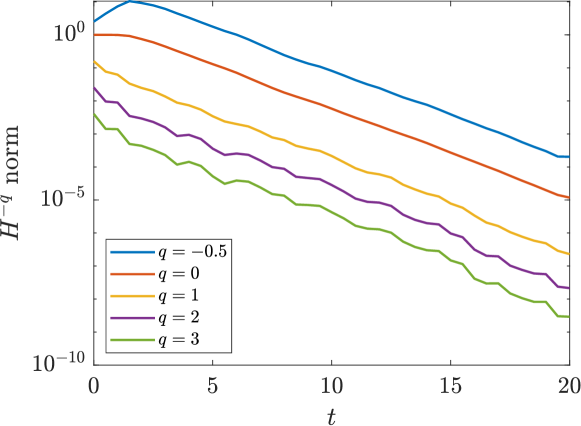
Figure 4. For the advection-diffusion equation (1.1) with $\bm{u}$ given by the random sine flow (3.7), the rate of decay of the mix-norms is independent of $q$. The the initial condition is $f^{0}(x)=\sqrt{2}\cos(2\pi x)$, and the diffusivity is $D=10^{-5}$.

In general, if $f^{t}$ is $q$-recurrent then the decay rate of the mix-norm is independent of $q$ in the following sense:

Theorem 3.

If $f^{t}$ is $q$-recurrent, then it is also $q^{\prime}$-recurrent for any $q^{\prime}>q$. Moreover, we have

$$\limsup_{t\to\infty}\frac{\mathopen{}\mathclose{{}\left\lVert f^{t}}\right\rVert_{\dot{H}^{-q^{\prime}}}}{\mathopen{}\mathclose{{}\left\lVert f^{t}}\right\rVert_{\dot{H}^{-q}}}>0\,.$$

Then together with the trivial estimate

$$\mathopen{}\mathclose{{}\left\lVert f^{t}}\right\rVert_{\dot{H}^{-q^{\prime}}}\leq\mathopen{}\mathclose{{}\left\lVert f^{t}}\right\rVert_{\dot{H}^{-q}}$$ (3.8)

we conclude that $\mathopen{}\mathclose{{}\left\lVert f^{t}}\right\rVert_{\dot{H}^{-q^{\prime}}}$ is Big-O but not Little-O of $\mathopen{}\mathclose{{}\left\lVert f^{t}}\right\rVert_{\dot{H}^{-q}}$.

Proof.

Since $f^{t}$ is $q$-recurrent, there is a finite set $I$ such that

$$0<\limsup_{t\to\infty}\frac{\mathopen{}\mathclose{{}\left\lVert P_{I}f^{t}}\right\rVert_{\dot{H}^{-q}}}{\mathopen{}\mathclose{{}\left\lVert f^{t}}\right\rVert_{\dot{H}^{-q}}}\,.$$ (3.9)

Say $I\subset[-R,R]$ for some $R\in\mathds{N}$. Then

$$\mathopen{}\mathclose{{}\left\lVert P_{I}f^{t}}\right\rVert_{\dot{H}^{-q}}\leq R^{(q^{\prime}-q)}\mathopen{}\mathclose{{}\left\lVert P_{I}f^{t}}\right\rVert_{\dot{H}^{-q^{\prime}}}\,.$$ (3.10)

Putting together Eqs. 3.8, 3.9 and 3.10 we obtain

$$0<R^{(q^{\prime}-q)}\limsup\frac{\mathopen{}\mathclose{{}\left\lVert P_{I}f^{t}}\right\rVert_{\dot{H}^{-q^{\prime}}}}{\mathopen{}\mathclose{{}\left\lVert f^{t}}\right\rVert_{\dot{H}^{-q^{\prime}}}}.$$

We conclude $f^{t}$ is $q^{\prime}$-recurrent. Moreover, the trivial estimate $\mathopen{}\mathclose{{}\left\lVert P_{I}f^{t}}\right\rVert_{\dot{H}^{-q^{\prime}}}\leq\mathopen{}\mathclose{{}\left\lVert f^{t}}\right\rVert_{\dot{H}^{-q^{\prime}}}$ together with Eqs. 3.9 and 3.10 imply

$$0<R^{(q^{\prime}-q)}\limsup\frac{\mathopen{}\mathclose{{}\left\lVert f^{t}}\right\rVert_{\dot{H}^{-q^{\prime}}}}{\mathopen{}\mathclose{{}\left\lVert f^{t}}\right\rVert_{\dot{H}^{-q}}}.$$ (3.11)

∎

One question for further investigation is whether a converse to the above theorem exists. That is, can we conclude $f^{t}$ is $q$-recurrent for a range of $q$ if the mix-norms decay at the same rate for the those $q$? Another question concerns the transition from $q$-transient to $q$-recurrent when including pulsed diffusion. Does $q$-recurrence imply an introduction of the Batchelor scale and anomalous dissipation [4, 28, 27]?

4. Proof of Theorem 1

We begin by generalizing the definition of $q$-recurrent functions to the notion of ‘$(q,h)$-recurrent’̃ functions.

Definition 2.

For positive functions $h(t)$, we say $f^{t}$ is $(q,h)$-recurrent if there exists a finite set $I\subset\mathds{Z}^{d}$ such that

$$\limsup_{t\to\infty}\frac{\mathopen{}\mathclose{{}\left\lVert P_{I}f^{t}}\right\rVert_{\dot{H}^{-q}}}{h}>0.$$ (4.1)

Functions that are not $(q,h)$-recurrent are called $(q,h)$-transient.

Lemma 1.

If $f^{t}$ is $(q,h)$-recurrent, then there is a function $g\in\dot{H}^{q}$ such that

$$\limsup_{t\to\infty}\frac{\mathopen{}\mathclose{{}\left|\mathopen{}\mathclose{{}\left\langle f^{t}\,,\,g}\right\rangle}\right|}{h}>0.$$

Moreover, $g\in\dot{H}^{\beta}$ for any $\beta\in\mathds{R}$ with

$$\mathopen{}\mathclose{{}\left\lVert g}\right\rVert_{\dot{H}^{\beta}}^{2}=2\sum\limits_{{\bm{k}}\in I}k^{2(\beta-q)}.$$ (4.2)

Proof.

There exists a constant $c>0$ and a sequence of times $t_{m}\to\infty$ where

$$\sum\limits_{{\bm{k}}\in I}|f_{\bm{k}}^{t_{m}}|^{2}\,k^{-2q}\geq c^{2}h^{2}(t_{m}).$$ (4.3)

Recall the signum function

$$\operatorname{sgn}x=\mathopen{}\mathclose{{}\left\{\begin{array}[]{ll}\phantom{-}1,&x\geq 0;\\ -1,&x<0.\end{array}}\right.$$ (4.4)

Now notice that for each fixed time $t_{m}$, $\{f^{t_{m}}_{\bm{k}}\}_{{\bm{k}}\in I}$ is a list of $|I|$ numbers in $\mathds{C}$. Write $f^{t_{m}}_{\bm{k}}=a_{\bm{k}}^{t_{m}}+ib_{\bm{k}}^{t_{m}}$ where $a_{\bm{k}}^{t_{m}}$ and $b_{\bm{k}}^{t_{m}}$ are real. Then $f^{t_{m}}_{\bm{k}}$ is found in one of the four quadrants of the complex plane, depending on the two possibilities for $\operatorname{sgn}a_{\bm{k}}^{t_{m}}$ and two possibilities for $\operatorname{sgn}b_{\bm{k}}^{t_{m}}$. Thus, $\{f^{t_{m}}_{\bm{k}}\}_{{\bm{k}}\in I}$ has $4^{|I|}$ possible states. Since we have an infinite sequence of times $t_{m}$, one of these states must occur infinitely many times. By taking a subsequence $t_{m_{\ell}}$, we can ensure $\{f^{t_{m_{\ell}}}_{\bm{k}}\}_{{\bm{k}}\in I}$ is the same state for all $\ell$. Let $\{(c_{\bm{k}},d_{\bm{k}})\}_{{\bm{k}}\in I}$ encode this state, meaning that $c_{\bm{k}}=\operatorname{sgn}a_{\bm{k}}^{t_{m_{\ell}}}$ and $d_{\bm{k}}=\operatorname{sgn}b_{\bm{k}}^{t_{m_{\ell}}}$ for all $\ell$. We see that $a_{\bm{k}}^{t_{m_{\ell}}}c_{\bm{k}}=\bigl{|}a_{\bm{k}}^{t_{m_{\ell}}}\bigr{|}$ and $b_{\bm{k}}^{t_{m_{\ell}}}d_{\bm{k}}=\bigl{|}b_{\bm{k}}^{t_{m_{\ell}}}\bigr{|}$ for all $\ell$. Let

$$g_{\bm{k}}=\mathopen{}\mathclose{{}\left\{\begin{array}[]{ll}\mathopen{}\mathclose{{}\left(c_{\bm{k}}+id_{\bm{k}}}\right)k^{-q},&{\bm{k}}\in I;\\ 0,&\text{otherwise}.\end{array}}\right.$$ (4.5)

Notice that $g\in\dot{H}^{\beta}$ because

$$\mathopen{}\mathclose{{}\left\lVert g}\right\rVert_{\dot{H}^{\beta}}^{2}=\sum|g_{\bm{k}}|^{2}\,k^{2\beta}=\sum\limits_{{\bm{k}}\in I}(|c_{\bm{k}}|^{2}+|d_{\bm{k}}|^{2})k^{-2q}k^{2\beta}=2\sum\limits_{{\bm{k}}\in I}k^{2(\beta-q)}<\infty$$ (4.6)

since $I$ is a finite set. We have

$$\sum f_{\bm{k}}^{t_{m_{\ell}}}~{}\bar{g}_{\bm{k}} =\sum\limits_{{\bm{k}}\in I}\mathopen{}\mathclose{{}\left(a_{\bm{k}}^{t_{m_{\ell}}}+ib_{\bm{k}}^{t_{m_{\ell}}}}\right)\mathopen{}\mathclose{{}\left(c_{\bm{k}}-id_{\bm{k}}}\right)~{}k^{-q}$$

$$=\sum\limits_{{\bm{k}}\in I}\mathopen{}\mathclose{{}\left(a_{\bm{k}}^{t_{m_{\ell}}}c_{\bm{k}}+b_{\bm{k}}^{t_{m_{\ell}}}d_{\bm{k}}+i\mathopen{}\mathclose{{}\left(b_{\bm{k}}^{t_{m_{\ell}}}c_{\bm{k}}-a_{\bm{k}}^{t_{m_{\ell}}}d_{\bm{k}}}\right)}\right)~{}k^{-q}$$

$$=\sum\limits_{{\bm{k}}\in I}\mathopen{}\mathclose{{}\left(\bigl{|}a_{\bm{k}}^{t_{m_{\ell}}}\bigr{|}+\bigl{|}b_{\bm{k}}^{t_{m_{\ell}}}\bigr{|}+i\mathopen{}\mathclose{{}\left(b_{\bm{k}}^{t_{m_{\ell}}}c_{\bm{k}}-a_{\bm{k}}^{t_{m_{\ell}}}d_{\bm{k}}}\right)}\right)~{}k^{-q}.$$

We conclude that

$$\mathopen{}\mathclose{{}\left|\mathopen{}\mathclose{{}\left\langle f^{t_{m_{\ell}}}\,,\,g}\right\rangle}\right| \geq\mathrm{Re}\sum f_{\bm{k}}^{t_{m_{\ell}}}~{}\bar{g}_{\bm{k}}$$

$$=\sum\limits_{{\bm{k}}\in I}\mathopen{}\mathclose{{}\left(\bigl{|}a_{\bm{k}}^{t_{m_{\ell}}}\bigr{|}+\bigl{|}b_{\bm{k}}^{t_{m_{\ell}}}\bigr{|}}\right)~{}k^{-q}$$

$$\geq\sum\limits_{{\bm{k}}\in I}\sqrt[]{\bigl{|}a_{\bm{k}}^{t_{m_{\ell}}}\bigr{|}^{2}+\bigl{|}b_{\bm{k}}^{t_{m_{\ell}}}\bigr{|}^{2}}~{}k^{-q}$$

$$=\sum\limits_{{\bm{k}}\in I}\mathopen{}\mathclose{{}\left|f_{\bm{k}}^{t_{m_{\ell}}}}\right|~{}k^{-q},$$

as desired. Lastly, we use dominance of $\ell^{2}$ by $\ell^{1}$ together with Eq. 4.3 to conclude $\mathopen{}\mathclose{{}\left|\mathopen{}\mathclose{{}\left\langle f^{t_{m_{\ell}}}\,,\,g}\right\rangle}\right|\geq c\,h(t_{m_{\ell}})$, $\forall m_{\ell}$. ∎

Lemma 1 characterizes the behavior of $(q,h)$-recurrent functions. We now develop the tool we need to further analyze $(q,h)$-transient functions.

Lemma 2.

Let $f^{t}$ be $(q,h)$-transient for some positive $h=\mathcal{O}\mathopen{}\mathclose{{}\left(\mathopen{}\mathclose{{}\left\lVert f^{t}}\right\rVert_{\dot{H}^{-q}}}\right)$. For any $\delta$ with $0<\delta<1$, there exist sets $I_{i}=\{{\bm{k}}\,|\,J_{i-1}<|{\bm{k}}|\leq J_{i}\}$ and a sequence of times $T_{i}\to\infty$ satisfying the following:

Property 1.

The set $I_{i}$ captures a significant proportion of the Fourier energy at time $T_{i}$, so that

$$\sum\limits_{{\bm{k}}\in I_{i}}\mathopen{}\mathclose{{}\left|f_{\bm{k}}^{T_{i}}}\right|^{2}\,k^{-2q}\geq(1-\delta)\mathopen{}\mathclose{{}\left\lVert f^{T_{i}}}\right\rVert_{\dot{H}^{-q}}^{2}\,.$$ (4.7)

Property 2.

Enough of the Fourier energy does not return to lower frequency modes, so that

$$\sum\limits_{|{\bm{k}}|\leq J_{i-1}}\mathopen{}\mathclose{{}\left|f_{\bm{k}}^{t}}\right|^{2}\,k^{-2q}\leq\delta\,h^{2}(t)\text{ for all }t\geq T_{i}\,.$$ (4.8)

Proof.

Base case: $i=1$. Since (by definition of absolute convergence)

$$\lim\limits_{J\to\infty}\sum\limits_{|{\bm{k}}|\leq J}\mathopen{}\mathclose{{}\left|f_{\bm{k}}^{0}}\right|^{2}\,k^{-2q}=\mathopen{}\mathclose{{}\left\lVert f^{0}}\right\rVert_{\dot{H}^{-q}}^{2}$$ (4.9)

there is a $J_{1}$ such that

$$\sum\limits_{|{\bm{k}}|\leq J_{1}}\mathopen{}\mathclose{{}\left|f_{\bm{k}}^{0}}\right|^{2}\,k^{-2q}\geq(1-\delta)\mathopen{}\mathclose{{}\left\lVert f^{0}}\right\rVert_{\dot{H}^{-q}}^{2}\,.$$ (4.10)

We see $I_{1}=\{{\bm{k}}\,|\,J_{0}<|{\bm{k}}|\leq J_{1}\}$ where $J_{0}=-1$ and $T_{1}=0$ therefore trivially satisfy Properties 1 and 2.

Induction step: Suppose that we are given $J_{i-2},J_{i-1}$ and $T_{i-1}$ that satisfy Properties 1 and 2. Since $h=\mathcal{O}\mathopen{}\mathclose{{}\left(\mathopen{}\mathclose{{}\left\lVert f^{t}}\right\rVert_{\dot{H}^{-q}}}\right)$, there is a $c>0$ and a time $T$ so that $h(t)\leq c\mathopen{}\mathclose{{}\left\lVert f^{t}}\right\rVert_{\dot{H}^{-q}}~{}\forall t\geq T$. Recall that $f^{t}$ is $(q,h)$-transient and so there does not exist a sequence $t_{m}\to\infty$ where

$$\sum\limits_{|{\bm{k}}|\leq J_{i-1}}\mathopen{}\mathclose{{}\left|f_{\bm{k}}^{t_{m}}}\right|^{2}\,k^{-2q}\geq\min(\delta,\delta/c^{2})~{}h^{2}(t_{m}),\quad\forall m.$$ (4.11)

We conclude that there exist $T_{i}$ with $T_{i}\geq T_{i-1}+1$ and $T_{i}\geq T$ such that Property 2 is satisfied. In particular, we have

$$\sum\limits_{|{\bm{k}}|\leq J_{i-1}}\mathopen{}\mathclose{{}\left|f_{\bm{k}}^{T_{i}}}\right|^{2}\,k^{-2q}<\delta/c^{2}~{}h^{2}(T_{i})\leq\delta\mathopen{}\mathclose{{}\left\lVert f^{T_{i}}}\right\rVert_{\dot{H}^{-q}}^{2}\,.$$ (4.12)

Hence,

$$\sum\limits_{|{\bm{k}}|>J_{i-1}}\mathopen{}\mathclose{{}\left|f_{\bm{k}}^{T_{i}}}\right|^{2}\,k^{-2q}>(1-\delta)\mathopen{}\mathclose{{}\left\lVert f^{T_{i}}}\right\rVert_{\dot{H}^{-q}}^{2},$$ (4.13)

and it follows that there is a $J_{i}$ large enough so that for $I_{i}=\{{\bm{k}}\,|\,J_{i-1}<|{\bm{k}}|<J_{i}\}$ we have

$$\sum\limits_{{\bm{k}}\in I_{i}}|f_{\bm{k}}^{T_{i}}|^{2}\,k^{-2q}\geq(1-\delta)\mathopen{}\mathclose{{}\left\lVert f^{T_{i}}}\right\rVert_{\dot{H}^{-q}}^{2}\,$$ (4.14)

which is Property 1. ∎

Having developed all of the tools we will need, we now prove Theorem 1 and, in the next section, Theorem 2.

See 1

Proof.

The forward direction is a special case of Lemma 1 with $h(t)=\mathopen{}\mathclose{{}\left\lVert f^{t}}\right\rVert_{\dot{H}^{-q}}$. We assume $f^{t}$ is $q$-transient and show $\mathopen{}\mathclose{{}\left\langle f^{t}\,,\,g}\right\rangle=o\mathopen{}\mathclose{{}\left(\mathopen{}\mathclose{{}\left\lVert f^{t}}\right\rVert_{\dot{H}^{-q}}}\right)$ for all $g\in\dot{H}^{q}$. We already know $\mathopen{}\mathclose{{}\left\langle f^{t}\,,\,g}\right\rangle=\mathcal{O}\mathopen{}\mathclose{{}\left(\mathopen{}\mathclose{{}\left\lVert f^{t}}\right\rVert_{\dot{H}^{-q}}}\right)$ for all $g\in\dot{H}^{q}$, so

$$\limsup_{t\to\infty}\frac{\mathopen{}\mathclose{{}\left|\mathopen{}\mathclose{{}\left\langle f^{t}\,,\,g}\right\rangle}\right|}{\mathopen{}\mathclose{{}\left\lVert f^{t}}\right\rVert_{\dot{H}^{-q}}}<\infty,\quad\forall g\in\dot{H}^{q}.$$ (4.15)

Seeking a contradiction, we suppose there exists a $g\in\dot{H}^{q}$ such that

$$\limsup_{t\to\infty}\frac{\mathopen{}\mathclose{{}\left|\mathopen{}\mathclose{{}\left\langle f^{t}\,,\,g}\right\rangle}\right|}{\mathopen{}\mathclose{{}\left\lVert f^{t}}\right\rVert_{\dot{H}^{-q}}}=C>0.$$ (4.16)

There is a sequence $t_{n}\to\infty$ such that

$$\mathopen{}\mathclose{{}\left|\mathopen{}\mathclose{{}\left\langle f^{t_{n}}\,,\,g}\right\rangle}\right|\geq\frac{C}{2}\mathopen{}\mathclose{{}\left\lVert f^{t_{n}}}\right\rVert_{\dot{H}^{-q}},\quad\forall n.$$ (4.17)

We will show that Eq. 4.17 implies that the Fourier coefficients of $g$ decay too slowly for $g$ to be in $\dot{H}^{q}$.

Since $g\in\dot{H}^{q}$, we can choose $\delta$ small enough that $\frac{C}{2}-2\sqrt{\delta}\mathopen{}\mathclose{{}\left\lVert g}\right\rVert_{\dot{H}^{q}}=C_{0}>0$. Applying Lemma 2 with $h(t)=\mathopen{}\mathclose{{}\left\lVert f^{t}}\right\rVert_{\dot{H}^{-q}}$, there exist sets $I_{i}=\{{\bm{k}}\,|\,J_{i-1}<|{\bm{k}}|\leq J_{i}\}$ and a sequence of times $T_{i}\to\infty$ (without loss of generality, say that $\{T_{i}\}$ is a subsequence of $\{t_{n}\}$ above) such that we have Properties 1 and 2. Property 1 implies

$$\sum\limits_{|{\bm{k}}|>J_{i}}\mathopen{}\mathclose{{}\left|f_{\bm{k}}^{T_{i}}}\right|^{2}\,k^{-2q}\leq\delta\mathopen{}\mathclose{{}\left\lVert f^{T_{i}}}\right\rVert_{\dot{H}^{-q}}^{2}\,.$$ (4.18)

Note that

$$\mathopen{}\mathclose{{}\left\langle f^{T_{i}}\,,\,g}\right\rangle =\sum_{j\geq 1}\sum_{{\bm{k}}\in I_{j}}f_{\bm{k}}^{T_{i}}~{}\bar{g}_{\bm{k}}$$

$$=\sum_{{\bm{k}}\in I_{i}}f_{\bm{k}}^{T_{i}}~{}\bar{g}_{\bm{k}}+E$$ (4.19)

where

$$E=\sum_{j\neq i}\sum_{{\bm{k}}\in I_{j}}f_{\bm{k}}^{T_{i}}~{}\bar{g}_{\bm{k}}=\sum_{j<i}\sum_{{\bm{k}}\in I_{j}}f_{\bm{k}}^{T_{i}}~{}\bar{g}_{\bm{k}}+\sum_{j>i}\sum_{{\bm{k}}\in I_{j}}f_{\bm{k}}^{T_{i}}~{}\bar{g}_{\bm{k}}=:E_{1}+E_{2}\,.$$ (4.20)

By the Cauchy–Schwarz inequality,

$$|E_{1}| \leq\mathopen{}\mathclose{{}\left(\sum_{j<i}\sum_{{\bm{k}}\in I_{j}}\mathopen{}\mathclose{{}\left|f_{\bm{k}}^{T_{i}}}\right|^{2}\,k^{-2q}}\right)^{1/2}\mathopen{}\mathclose{{}\left(\sum_{j<i}\sum_{{\bm{k}}\in I_{j}}\mathopen{}\mathclose{{}\left|g_{\bm{k}}}\right|^{2}\,k^{2q}}\right)^{1/2}.$$ (4.21)

Applying Property 2 (with $t=T_{i}$), we have

$$|E_{1}|\leq\sqrt{\delta}\mathopen{}\mathclose{{}\left\lVert f^{T_{i}}}\right\rVert_{\dot{H}^{-q}}\mathopen{}\mathclose{{}\left\lVert g}\right\rVert_{\dot{H}^{q}}\,.$$ (4.22)

Similarly, by Cauchy–Schwarz and Eq. 4.18, we have

$$|E_{2}|\leq\sqrt{\delta}\mathopen{}\mathclose{{}\left\lVert f^{T_{i}}}\right\rVert_{\dot{H}^{-q}}\mathopen{}\mathclose{{}\left\lVert g}\right\rVert_{\dot{H}^{q}}$$ (4.23)

and therefore

$$\mathopen{}\mathclose{{}\left|\mathopen{}\mathclose{{}\left\langle f^{T_{i}}\,,\,g}\right\rangle}\right|\leq\mathopen{}\mathclose{{}\left|\sum_{{\bm{k}}\in I_{i}}f_{\bm{k}}^{T_{i}}~{}\bar{g}_{\bm{k}}}\right|+2\sqrt{\delta}\mathopen{}\mathclose{{}\left\lVert f^{T_{i}}}\right\rVert_{\dot{H}^{-q}}\mathopen{}\mathclose{{}\left\lVert g}\right\rVert_{\dot{H}^{q}}\,.$$ (4.24)

Putting together Eqs. 4.17 and 4.24, we have

$$\mathopen{}\mathclose{{}\left(\frac{C}{2}-2\sqrt{\delta}\mathopen{}\mathclose{{}\left\lVert g}\right\rVert_{\dot{H}^{q}}}\right)\mathopen{}\mathclose{{}\left\lVert f^{T_{i}}}\right\rVert_{\dot{H}^{-q}}\leq\mathopen{}\mathclose{{}\left|\sum_{{\bm{k}}\in I_{i}}f_{\bm{k}}^{T_{i}}~{}\bar{g}_{\bm{k}}}\right|.$$ (4.25)

Applying Cauchy–Schwarz to the right-hand side of Eq. 4.25 we have

$$C_{0}\mathopen{}\mathclose{{}\left\lVert f^{T_{i}}}\right\rVert_{\dot{H}^{-q}} \leq\mathopen{}\mathclose{{}\left(\sum_{{\bm{k}}\in I_{i}}\mathopen{}\mathclose{{}\left|f_{\bm{k}}^{T_{i}}}\right|^{2}\,k^{-2q}}\right)^{1/2}\mathopen{}\mathclose{{}\left(\sum_{{\bm{k}}\in I_{i}}\mathopen{}\mathclose{{}\left|g_{\bm{k}}}\right|^{2}\,k^{2q}}\right)^{1/2}$$ (4.26)

$$\leq\mathopen{}\mathclose{{}\left\lVert f^{T_{i}}}\right\rVert_{\dot{H}^{-q}}\mathopen{}\mathclose{{}\left(\sum_{{\bm{k}}\in I_{i}}\mathopen{}\mathclose{{}\left|g_{\bm{k}}}\right|^{2}\,k^{2q}}\right)^{1/2}.$$ (4.27)

Therefore

$$\sum_{{\bm{k}}\in I_{i}}\mathopen{}\mathclose{{}\left|g_{\bm{k}}}\right|^{2}\,k^{2q}\geq C_{0}^{2},\quad\forall i\,.$$ (4.28)

This shows that the coefficients of $g$ are large on sets $I_{i}$ and we have

$$\mathopen{}\mathclose{{}\left\lVert g}\right\rVert_{\dot{H}^{q}}^{2}=\sum_{i}\sum_{{\bm{k}}\in I_{i}}\mathopen{}\mathclose{{}\left|g_{\bm{k}}}\right|^{2}\,k^{2q}\geq\sum_{i}C_{0}^{2}=\infty.$$ (4.29)

We conclude that $g$ is not in $\dot{H}^{q}$ — a contradiction. ∎

5. Proof of Theorem 2

See 2

Proof of Theorem 2.

If $f^{t}$ is $(q,h)$-recurrent, then we are done by Lemma 1, so say $f^{t}$ is $(q,h)$-transient. Take some $\delta<1/3$ and apply Lemma 2 to construct sets $\mathopen{}\mathclose{{}\left\{I_{i}}\right\}_{i=1}^{\infty}$ and a sequence $\mathopen{}\mathclose{{}\left\{T_{i}}\right\}_{i=1}^{\infty}$. Let $\mathopen{}\mathclose{{}\left\{T_{i_{\ell}}}\right\}_{\ell=1}^{\infty}$ be a subsequence of $\mathopen{}\mathclose{{}\left\{T_{i}}\right\}_{i=1}^{\infty}$ satisfying

$$\sum\limits_{\ell>L}i_{\ell}/\leq\delta^{2}\,i_{L}/.$$ (5.1)

and

$$\sum\limits i_{\ell}/\leq\delta.$$ (5.2)

This can be done since $h(t)=o(\mathopen{}\mathclose{{}\left\lVert f^{t}}\right\rVert_{\dot{H}^{-q}})$. Let $g$ be the function with Fourier coefficients given by

$$g_{\bm{k}}=\mathopen{}\mathclose{{}\left\{\begin{array}[]{ll}f_{\bm{k}}^{T_{i_{\ell}}}k^{-2q}\mathopen{}\mathclose{{}\left\lVert f^{T_{i_{\ell}}}}\right\rVert_{\dot{H}^{-q}}^{-2}h(T_{i_{\ell}})&{\bm{k}}\in I_{i_{\ell}}\,;\\ 0&\text{otherwise}.\\ \end{array}}\right.$$ (5.3)

Eq. 5.2 allows us to conclude that $g\in\dot{H}^{q}$:

$$\mathopen{}\mathclose{{}\left\lVert g}\right\rVert_{\dot{H}^{q}}^{2} =\sum\mathopen{}\mathclose{{}\left|g_{\bm{k}}}\right|^{2}\,k^{2q}$$

$$=\sum\limits_{i_{\ell}}\sum\limits_{{\bm{k}}\in I_{i_{\ell}}}\mathopen{}\mathclose{{}\left|f_{\bm{k}}^{T_{i_{\ell}}}}\right|^{2}\,k^{-4q}\mathopen{}\mathclose{{}\left\lVert f^{T_{i_{\ell}}}}\right\rVert_{\dot{H}^{-q}}^{-4}h^{2}(T_{i_{\ell}})~{}k^{2q}$$

$$=\sum\limits_{i_{\ell}}\mathopen{}\mathclose{{}\left\lVert f^{T_{i_{\ell}}}}\right\rVert_{\dot{H}^{-q}}^{-4}h^{2}(T_{i_{\ell}})\mathopen{}\mathclose{{}\left(\sum\limits_{{\bm{k}}\in I_{i_{\ell}}}\mathopen{}\mathclose{{}\left|f_{\bm{k}}^{T_{i_{\ell}}}}\right|^{2}\,k^{-2q}}\right)$$

$$\leq\sum\limits_{i_{\ell}}\mathopen{}\mathclose{{}\left\lVert f^{T_{i_{\ell}}}}\right\rVert_{\dot{H}^{-q}}^{-2}h^{2}(T_{i_{\ell}}).$$

We will now finish the proof by showing $\mathopen{}\mathclose{{}\left|\mathopen{}\mathclose{{}\left\langle f^{T_{i_{\ell}}}\,,\,g}\right\rangle}\right|\geq(1-3\delta)~{}h(T_{i_{\ell}})$. We begin with some notation. Split the following sum into two parts:

$$\mathopen{}\mathclose{{}\left\langle f^{T_{i_{\ell}}}\,,\,g}\right\rangle =\sum\limits_{j_{\ell}}\sum\limits_{{\bm{k}}\in I_{j_{\ell}}}f^{T_{i_{\ell}}}_{\bm{k}}~{}\overline{f_{\bm{k}}^{T_{j_{\ell}}}}k^{-2q}\mathopen{}\mathclose{{}\left\lVert f^{T_{j_{\ell}}}}\right\rVert_{\dot{H}^{-q}}^{-2}h(T_{j_{\ell}})$$

$$=S^{T_{i_{\ell}}}+E^{T_{i_{\ell}}},$$

where $S^{T_{i_{\ell}}}$ is the sum when $j_{\ell}=i_{\ell}$ :

$$S^{T_{i_{\ell}}} =\sum\limits_{j_{\ell}=i_{\ell}}\sum\limits_{{\bm{k}}\in I_{i_{\ell}}}f^{T_{i_{\ell}}}_{\bm{k}}~{}\overline{f_{\bm{k}}^{T_{j_{\ell}}}}k^{-2q}\mathopen{}\mathclose{{}\left\lVert f^{T_{j_{\ell}}}}\right\rVert_{\dot{H}^{-q}}^{-2}h(T_{j_{\ell}})$$

$$=\sum\limits_{{\bm{k}}\in I_{i_{\ell}}}\mathopen{}\mathclose{{}\left|f^{T_{i_{\ell}}}_{\bm{k}}}\right|^{2}~{}k^{-2q}~{}\mathopen{}\mathclose{{}\left\lVert f^{T_{i_{\ell}}}}\right\rVert_{\dot{H}^{-q}}^{-2}~{}h(T_{i_{\ell}}),$$

and $E^{T_{i_{\ell}}}$ is the sum over $j_{\ell}\neq i_{\ell}$ :

$$E^{T_{i_{\ell}}}=\sum\limits_{j_{\ell}\neq i_{\ell}}\sum\limits_{{\bm{k}}\in I_{j_{\ell}}}f^{T_{i_{\ell}}}_{\bm{k}}~{}\overline{f_{\bm{k}}^{T_{j_{\ell}}}}k^{-2q}\mathopen{}\mathclose{{}\left\lVert f^{T_{j_{\ell}}}}\right\rVert_{\dot{H}^{-q}}^{-2}h(T_{j_{\ell}})\,.$$ (5.4)

The idea is that $g_{\bm{k}}$ is constructed to agree well with $f^{T_{i_{\ell}}}_{\bm{k}}$ when ${\bm{k}}\in I_{i_{\ell}}$. We will show that $S^{T_{i_{\ell}}}$ dominates the error $E^{T_{i_{\ell}}}$. Consider $j_{\ell}<i_{\ell}$ and $j_{\ell}>i_{\ell}$ separately in Eq. 5.4; taking absolute value, we have

$$\mathopen{}\mathclose{{}\left|E^{T_{i_{\ell}}}}\right|\leq\sum\limits_{j_{\ell}\neq i_{\ell}}\sum\limits_{{\bm{k}}\in I_{j_{\ell}}}\mathopen{}\mathclose{{}\left|f^{T_{i_{\ell}}}_{\bm{k}}}\right|\mathopen{}\mathclose{{}\left|f^{T_{j_{\ell}}}_{\bm{k}}}\right|~{}k^{-2q}~{}\mathopen{}\mathclose{{}\left\lVert f^{T_{j_{\ell}}}}\right\rVert_{\dot{H}^{-q}}^{-2}~{}h(T_{j_{\ell}})$$ (5.5)

and let $E^{T_{i_{\ell}}}_{1}$ be the sum over $j_{\ell}<i_{\ell}$ :

$$E^{T_{i_{\ell}}}_{1}:=\sum\limits_{j_{\ell}<i_{\ell}}\sum\limits_{{\bm{k}}\in I_{j_{\ell}}}\mathopen{}\mathclose{{}\left|f^{T_{i_{\ell}}}_{\bm{k}}}\right|\mathopen{}\mathclose{{}\left|f^{T_{j_{\ell}}}_{\bm{k}}}\right|~{}k^{-2q}~{}\mathopen{}\mathclose{{}\left\lVert f^{T_{j_{\ell}}}}\right\rVert_{\dot{H}^{-q}}^{-2}~{}h(T_{j_{\ell}})\,.$$ (5.6)

Similarly define $E^{T_{i_{\ell}}}_{2}$ to be the sum over $j_{\ell}>i_{\ell}$ :

$$E^{T_{i_{\ell}}}_{2}:=\sum\limits_{j_{\ell}>i_{\ell}}\sum\limits_{{\bm{k}}\in I_{j_{\ell}}}\mathopen{}\mathclose{{}\left|f^{T_{i_{\ell}}}_{\bm{k}}}\right|\mathopen{}\mathclose{{}\left|f^{T_{j_{\ell}}}_{\bm{k}}}\right|~{}k^{-2q}~{}\mathopen{}\mathclose{{}\left\lVert f^{T_{j_{\ell}}}}\right\rVert_{\dot{H}^{-q}}^{-2}~{}h(T_{j_{\ell}})\,.$$ (5.7)

We now bound $E^{T_{i_{\ell}}}_{1}$ using the Cauchy–Schwarz inequality:

$$E^{T_{i_{\ell}}}_{1} \leq\mathopen{}\mathclose{{}\left(\sum\limits_{j_{\ell}<i_{\ell}}\sum\limits_{{\bm{k}}\in I_{j_{\ell}}}\mathopen{}\mathclose{{}\left|f_{\bm{k}}^{T_{i_{\ell}}}}\right|^{2}k^{-2q}}\right)^{1/2}\mathopen{}\mathclose{{}\left(\sum\limits_{j_{\ell}<i_{\ell}}\sum\limits_{{\bm{k}}\in I_{j_{\ell}}}\mathopen{}\mathclose{{}\left|f_{\bm{k}}^{T_{j_{\ell}}}}\right|^{2}k^{-2q}\mathopen{}\mathclose{{}\left\lVert f^{T_{j_{\ell}}}}\right\rVert_{\dot{H}^{-q}}^{-4}~{}h^{2}(T_{j_{\ell}})}\right)^{1/2}$$

$$\leq\mathopen{}\mathclose{{}\left(\sum\limits_{j_{\ell}<i_{\ell}}\sum\limits_{{\bm{k}}\in I_{j_{\ell}}}\mathopen{}\mathclose{{}\left|f_{\bm{k}}^{T_{i_{\ell}}}}\right|^{2}k^{-2q}}\right)^{1/2}\mathopen{}\mathclose{{}\left(\sum\limits_{j_{\ell}<i_{\ell}}\mathopen{}\mathclose{{}\left\lVert f^{T_{j_{\ell}}}}\right\rVert_{\dot{H}^{-q}}^{-2}~{}h^{2}(T_{j_{\ell}})}\right)^{1/2}.$$

We use Property 2 from Lemma 2 to bound the first factor and Eq. 5.2 to bound the second factor:

$$E^{T_{i_{\ell}}}_{1}\leq\mathopen{}\mathclose{{}\left(\delta h^{2}(T_{i_{\ell}})}\right)^{1/2}\mathopen{}\mathclose{{}\left(\delta}\right)^{1/2}=\delta\,h(T_{i_{\ell}}).$$ (5.8)

We similarly bound $E^{T_{i_{\ell}}}_{2}$:

$$E^{T_{i_{\ell}}}_{2} \leq\mathopen{}\mathclose{{}\left(\sum\limits_{j_{\ell}>i_{\ell}}\sum\limits_{{\bm{k}}\in I_{j_{\ell}}}\mathopen{}\mathclose{{}\left|f_{\bm{k}}^{T_{i_{\ell}}}}\right|^{2}k^{-2q}}\right)^{1/2}\mathopen{}\mathclose{{}\left(\sum\limits_{j_{\ell}>i_{\ell}}\sum\limits_{{\bm{k}}\in I_{j_{\ell}}}\mathopen{}\mathclose{{}\left|f_{\bm{k}}^{T_{j_{\ell}}}}\right|^{2}k^{-2q}\mathopen{}\mathclose{{}\left\lVert f^{T_{j_{\ell}}}}\right\rVert_{\dot{H}^{-q}}^{-4}~{}h^{2}(T_{j_{\ell}})}\right)^{1/2}$$

$$\leq\mathopen{}\mathclose{{}\left\lVert f^{T_{i_{\ell}}}}\right\rVert_{\dot{H}^{-q}}\mathopen{}\mathclose{{}\left(\sum\limits_{j_{\ell}>i_{\ell}}\mathopen{}\mathclose{{}\left\lVert f^{T_{j_{\ell}}}}\right\rVert_{\dot{H}^{-q}}^{-2}~{}h^{2}(T_{j_{\ell}})}\right)^{1/2}.$$

Using Eq. 5.1, we find

$$E^{T_{i_{\ell}}}_{2}\leq\mathopen{}\mathclose{{}\left\lVert f^{T_{i_{\ell}}}}\right\rVert_{\dot{H}^{-q}}\mathopen{}\mathclose{{}\left(\delta^{2}\mathopen{}\mathclose{{}\left(\frac{h(T_{i_{\ell}})}{\mathopen{}\mathclose{{}\left\lVert f^{T_{i_{\ell}}}}\right\rVert_{\dot{H}^{-q}}}}\right)^{2}}\right)^{1/2}=\delta~{}h(T_{i_{\ell}})$$ (5.9)

and therefore

$$\mathopen{}\mathclose{{}\left\langle f^{T_{i_{\ell}}}\,,\,g}\right\rangle =S^{T_{i_{\ell}}}+E^{T_{i_{\ell}}}$$

$$\geq S^{T_{i_{\ell}}}-E^{T_{i_{\ell}}}_{1}-E^{T_{i_{\ell}}}_{2}$$

$$\geq S^{T_{i_{\ell}}}-\delta~{}h(T_{i_{\ell}})-\delta~{}h(T_{i_{\ell}}).$$

Again using Property 1 from Lemma 2 that the set $I_{i_{\ell}}$ captures a large proportion of the Sobolev norm, we conclude

$$\mathopen{}\mathclose{{}\left\langle f^{T_{i_{\ell}}}\,,\,g}\right\rangle \geq(1-\delta)\mathopen{}\mathclose{{}\left\lVert f^{T_{i_{\ell}}}}\right\rVert_{\dot{H}^{-q}}^{2}\mathopen{}\mathclose{{}\left\lVert f^{T_{i_{\ell}}}}\right\rVert_{\dot{H}^{-q}}^{-2}~{}h(T_{i_{\ell}})-2\delta~{}h(T_{i_{\ell}})$$

$$=\mathopen{}\mathclose{{}\left(1-3\delta}\right)~{}h(T_{i_{\ell}}).$$

∎

References

- Bedrossian and He [2019] J. Bedrossian and S. He. Inviscid damping and enhanced dissipation of the boundary layer for 2D Navier-Stokes linearized around Couette flow in a channel, 2019. https://arxiv.org/abs/1909.07230.
- Bedrossian et al. [2019a] J. Bedrossian, A. Blumenthal, and S. Punshon-Smith. Almost-sure exponential mixing of passive scalars by the stochastic Navier-Stokes equations, 2019a. https://arxiv.org/abs/1905.03869.
- Bedrossian et al. [2019b] J. Bedrossian, A. Blumenthal, and S. Punshon-Smith. Almost-sure enhanced dissipation and uniform-in-diffusivity exponential mixing for advection-diffusion by stochastic Navier-Stokes, 2019b. https://arxiv.org/abs/1911.01561.
- Bedrossian et al. [2019c] J. Bedrossian, A. Blumenthal, and S. Punshon-Smith. The Batchelor spectrum of passive scalar turbulence in stochastic fluid mechanics, 2019c. https://arxiv.org/abs/1911.11014.
- Chernov [1998] N. Chernov. Markov approximations and decay of correlations for Anosov flows. Ann. Math., 147(2):269–324, 1998.
- Constantin et al. [2008] P. Constantin, A. Kiselev, L. Ryzhik, and A. Zlatos̆. Diffusion and mixing in fluid flow. Ann. Math., 168(2):643–674, 2008.
- Coti Zelati [2019] M. Coti Zelati. Stable mixing estimates in the infinite Péclet number limit, 2019. https://arxiv.org/abs/1909.01310v1.
- Coti Zelati et al. [2018] M. Coti Zelati, M. G. Delgadino, and T. M. Elgindi. On the relation between enhanced dissipation time-scales and mixing rates. Comm. Pure Appl. Math., 2018. doi: 10.1002/cpa.21831. In press.
- Doering and Thiffeault [2006] C. R. Doering and J.-L. Thiffeault. Multiscale mixing efficiencies for steady sources. Phys. Rev. E, 74(2):025301(R), 2006.
- Dolgopyat [1998] D. Dolgopyat. On decay of correlations in Anosov flows. Ann. Math., 147(2):357–390, 1998.
- Elgindi and Zlatos̆ [2018] T. Elgindi and A. Zlatos̆. Universal mixers in all dimensions. September 2018.
- Feng and Iyer [2019] Y. Feng and G. Iyer. Dissipation enhancement by mixing. Nonlinearity, 32(5):1810–1851, April 2019.
- Folland [1999] Gerald B. Folland. Real Analysis: Modern Techniques and Their Applications. Wiley, New York, second edition, 1999.
- Hebey [2000] Emmanuel Hebey. Nonlinear Analysis on Manifolds: Sobolev Spaces and Inequalities. Courant, New York, first edition, 2000.
- Iyer et al. [2014] G. Iyer, A. Kiselev, and X. Xu. Lower bounds on the mix norm of passive scalars advected by incompressible enstrophy-constrained flows. Nonlinearity, 27(5):973–985, 2014. doi: 10.1088/0951-7715/27/5/973.
- Kiselev and Xu [2016] A. Kiselev and X. Xu. Suppression of chemotactic explosion by mixing. Arch. Rational Mech. Anal., 222(2):1077–1112, 2016. doi: 10.1007/s00205-016-1017-8.
- Kiselev et al. [2008] A. Kiselev, R. Shterenberg, and A. Zlatos̆. Relaxation enhancement by time-periodic flows. Indiana Univ. Math. J., 57:2137–2152, 2008.
- Lin et al. [2010] Z. Lin, K. Boďová, and C. R. Doering. Models & measures of mixing & effective diffusion. Discr. Cont. Dyn. Sys., 28(1):259–274, September 2010. doi: 10.3934/dcds.2010.28.259.
- Lin et al. [2011] Z. Lin, C. R. Doering, and J.-L. Thiffeault. Optimal stirring strategies for passive scalar mixing. J. Fluid Mech., 675:465–476, May 2011. doi: 10.1017/S0022112011000292.
- Liverani [1995] C. Liverani. Decay of correlations. Ann. Math., 142:239–301, September 1995. doi: 10.2307/2118636.
- Lunasin et al. [2012] E. Lunasin, Z. Lin, A. Novikov, A. Mazzucato, and C. R. Doering. Optimal mixing and optimal stirring for fixed energy, fixed power, or fixed palenstrophy flows. J. Math. Phys., 53:115611, 10.1063/1.4752098 2012.
- Lunasin et al. [2013] E. Lunasin, Z. Lin, A. Novikov, A. Mazzucato, and C. R. Doering. Erratum: “optimal mixing and optimal stirring for fixed energy, fixed power, or fixed palenstrophy flows”. J. Math. Phys., 54:079903, 10.1063/1.4816334 2013.
- Marcotte and Caulfield [2018] F. Marcotte and C. P. Caulfield. Optimal mixing in 2D stratified plane Poiseuille flow at finite Péclet and Richardson numbers. J. Fluid Mech., 853:359–385, 2018.
- Mathew et al. [2003] G. Mathew, I. Mezić, and L. Petzold. A multiscale measure for mixing and its applications. In Proc. Conf. on Decision and Control, Maui, HI. IEEE, December 2003.
- Mathew et al. [2005] G. Mathew, I. Mezić, and L. Petzold. A multiscale measure for mixing. Physica D, 211(1-2):23–46, November 2005.
- Mathew et al. [2007] G. Mathew, I. Mezić, S. Grivopoulos, U. Vaidya, and L. Petzold. Optimal control of mixing in Stokes fluid flows. J. Fluid Mech., 580:261–281, jun 2007.
- Miles and Doering [2018a] C. J. Miles and C. R. Doering. Diffusion-limited mixing by incompressible flows. Nonlinearity, 31(5):2346–2359, 2018a. doi: 10.1088/1361-6544/aab1c8.
- Miles and Doering [2018b] C. J. Miles and C. R. Doering. A shell model for optimal mixing. J. Nonlinear Sci., 28(2):2153–2186, 2018b. doi: 10.1007/s00332-017-9400-7.
- Pierrehumbert [1994] R. T. Pierrehumbert. Tracer microstructure in the large-eddy dominated regime. Chaos, Solitons and Fractals, 4:1091–1110, 1994.
- Pollicott [1981] M. Pollicott. On the rate of mixing of Axiom A flows. Invent. Math., 81:413–426, 1981.
- Shaw et al. [2007] T. A. Shaw, J.-L. Thiffeault, and C. R. Doering. Stirring up trouble: Multi-scale mixing measures for steady scalar sources. Physica D, 231:143–164, 2007.
- Sturman et al. [2006] R. Sturman, J. M. Ottino, and S. Wiggins. The Mathematical Foundations of Mixing: The Linked Twist Map as a Paradigm in Applications: Micro to Macro, Fluids to Solids. Cambridge University Press, Cambridge, U.K., 2006.
- Thiffeault [2012] J.-L. Thiffeault. Using multiscale norms to quantify mixing and transport. Nonlinearity, 25(2):R1–R44, February 2012. doi: 10.1088/0951-7715/25/2/R1.
- Thiffeault and Doering [2011] J.-L. Thiffeault and C. R. Doering. The mixing efficiency of open flows. Physica D, 240:180–185, January 2011.
- Thiffeault et al. [2004] J.-L. Thiffeault, C. R. Doering, and J. D. Gibbon. A bound on mixing efficiency for the advection-diffusion equation. J. Fluid Mech., 521:105–114, 2004.
- Vermach and Caulfield [2018] L. Vermach and C. P. Caulfield. Optimal mixing in three-dimensional plane Poiseuille flow at high Péclet number. J. Fluid Mech., 850:875–923, September 2018.
- Yao and Zlatos̆ [2017] Y. Yao and A. Zlatos̆. Mixing and un-mixing by incompressible flows. J. Eur. Math. Soc., 19(7):1911–1948, 2017. doi: 10.4171/JEMS/709.
- Young [1999] L.-S. Young. Recurrence times and rates of mixing. 110:153–188, 1999.
- Zillinger [2019] C. Zillinger. On geometric and analytic mixing scales: comparability and convergence rates for transport problems. Pure and Appl. Analysis, 1:543–570, 2019.