The Pre-Explosion Mass Distribution of Hydrogen-Poor Superluminous Supernova Progenitors and New Evidence for a Mass-Spin Correlation

Abstract

Despite indications that superluminous supernovae (SLSNe) originate from massive progenitors, the lack of a uniformly analyzed statistical sample has so far prevented a detailed view of the progenitor mass distribution. Here we present and analyze the pre-explosion mass distribution of hydrogen-poor SLSN progenitors as determined from uniformly modelled light curves of 62 events. We construct the distribution by summing the ejecta mass posteriors of each event, using magnetar light curve models presented in our previous works (and using a nominal neutron star remnant mass). The resulting distribution spans $3.6-40$ M_⊙, with a sharp decline at lower masses, and is best fit by a broken power law described by ${\rm d}N/{\rm dlog}M\propto M^{-0.41\pm 0.06}$ at $3.6-8.6$ M_⊙ and $\propto M^{-1.26\pm 0.06}$ at $8.6-40$ M_⊙. We find that observational selection effects cannot account for the shape of the distribution. Relative to Type Ib/c SNe, the SLSN mass distribution extends to much larger masses and has a different power-law shape, likely indicating that the formation of a magnetar allows more massive stars to explode as some of the rotational energy accelerates the ejecta. Comparing the SLSN distribution with predictions from single and binary star evolution models, we find that binary models for a metallicity of $Z\lesssim 1/3$ Z_⊙ are best able to reproduce its broad shape, in agreement with the preference of SLSNe for low metallicity environments. Finally, we uncover a correlation between the pre-explosion mass and the magnetar initial spin period, where SLSNe with low masses have slower spins, a trend broadly consistent with the effects of angular momentum transport evident in models of rapidly-rotating carbon-oxygen stars.

1 Introduction

The power source and progenitors of hydrogen-poor superluminous supernovae (Type I SLSNe; hereafter referred to as SLSNe) have remained a topic of intense debate since their discovery a decade ago (Gal-Yam et al., 2009; Pastorello et al., 2010; Chomiuk et al., 2011; Quimby et al., 2011; Gal-Yam, 2012), in part because of the order of magnitude spread in their peak luminosities and durations (Nicholl et al., 2015b; Lunnan et al., 2018a; De Cia et al., 2018; Angus et al., 2019). This has led to the suggestion of multiple energy sources (e.g., Gal-Yam, 2012), including abundant production of radioactive material and large ejecta masses from pair-instability explosions (PISNe; Heger & Woosley 2002), interaction of the SN ejecta with a dense circumstellar medium (CSM) that spans a range of mass loss rates and timescales (Chevalier & Irwin, 2011; Chatzopoulos et al., 2013), and powering by a magnetar central engine (Kasen & Bildsten, 2010; Woosley, 2010). Indeed, for the latter case it has been shown that explosions with ejecta masses of $M_{\rm ej}\sim 2-20$ M_⊙ that produce magnetars with initial spins of $P\sim 1-10$ ms and magnetic fields of $B\sim 10^{13}-10^{15}$ G can explain the observed range of peak luminosities and durations (Inserra et al., 2013; Nicholl et al., 2014, 2017b; Liu et al., 2017; Yu et al., 2017). In addition, late-time observations of SN 2015bn indicate a light curve flattening consistent with the power-law spin down of a magnetar (Nicholl et al., 2018). Still, detailed light curve features such as post-peak undulations (Nicholl et al., 2016a; Inserra et al., 2017; Blanchard et al., 2018) and early time bumps (Leloudas et al., 2012; Nicholl et al., 2015a; Smith et al., 2016; Nicholl, & Smartt, 2016; Angus et al., 2019) remain to be understood.

Unlike the other possible models, the magnetar interpretation is also supported by early-time ultraviolet/optical spectra (Dessart et al., 2012; Mazzali et al., 2016; Nicholl et al., 2017a) and by late-time optical nebular spectra, which show a remarkable similarity to broad-lined Type Ic SNe (SNe Ic-BL), in particular those associated with long gamma-ray bursts (LGRBs; Milisavljevic et al. 2013; Nicholl et al. 2016b, 2019; Jerkstrand et al. 2016, 2017). In addition, late-time radio emission detected at the position of PTF10hgi, the first such detection for a SLSN, has been shown to be consistent with expectations from a magnetar wind nebula (Eftekhari et al., 2019). On the other hand, there is currently no unambiguous case of a PISN origin for a SLSN. Similarly, while there is evidence for CSM interaction in a handful of events (Yan et al., 2017), including possibly the aforementioned light curve bumps, the inferred masses of this CSM are not sufficient to explain the peak luminosity and duration of SLSN light curves. While some CSM interaction likely contributes to the diversity of SLSNe, the spectroscopic properties are difficult to reconcile with a model in which CSM interaction is the dominant power source

Following this recent progress in understanding the power source in SLSNe, a key outstanding question is what types of progenitors can produce them. Given the lack of hydrogen and helium in the spectra of SLSNe, their progenitors are likely similar to those of other hydrogen-poor explosions such as Type Ib/c SNe (e.g., Pastorello et al. 2010) and LGRBs. The low volumetric rate of SLSNe compared to the overall Type Ib/c SN rate (Prajs et al., 2017), and their preference for low metallicity dwarf host galaxies (Chen et al., 2013; Lunnan et al., 2014; Leloudas et al., 2015; Perley et al., 2016; Schulze et al., 2018) points to a closer association with LGRB progenitors (another point in support of an engine-powered origin for SLSNe). In addition, a few SLSNe have exhibited direct links with LGRBs and SNe Ic-BL (Greiner et al., 2015; Blanchard et al., 2019) and on average SLSNe have absorption velocities similar to those of SNe Ic-BL (Liu et al., 2017). However, the details of this connection remain unclear.

Within the context of energy sources, progenitor properties, and the relation of SLSNe to other stripped SNe, it is essential to determine the distribution of pre-explosion progenitor masses, or nearly equivalently the ejecta masses. Moreover, within the context of the magnetar model, it is equally critical to assess any correlations between the engine and explosion properties, which may shed light on the conditions for SLSN production. Such a study requires a uniform analysis of a sufficiently large sample, which is now emerging from large-scale surveys such as the Pan-STARRS1 Medium-Deep Survey (Lunnan et al., 2018a), the Palomar Transient Factory (De Cia et al., 2018), the Dark Energy Survey (Angus et al., 2019), and the Zwicky Transient Facility (Lunnan et al., 2019).

Here we analyze the multi-band light curves of 62 SLSNe at $z\approx 0.06-1.6$ using the magnetar model (implemented in the light curve fitting code MOSFiT; Guillochon et al. 2018) to determine the ejecta mass distribution as a proxy for the progenitor mass distribution at the time of explosion, as well as to explore underlying correlations between the explosion and engine properties. Our study builds on the work and models of Nicholl et al. (2017b), which was focused on a smaller sample of 38 SLSNe, and Villar et al. (2018) which was focused on assessing SLSN science with the Large Synoptic Survey Telescope. We furthermore utilize simulated SLSN light curves with the same models to assess and account for the impact of observational selection biases in the existing SLSN sample.

The paper is structured as follows. In §2 we present the SLSN sample. In §3 we determine and analyze the progenitor mass distribution and compare it to Type Ib/c SNe and to massive star (single and binary) evolutionary models. In §4 we present evidence for a correlation between the ejecta mass and magnetar initial spin. In §5 we discuss the implications for our understanding of SLSN progenitors, and we conclude in §6.

2 SLSN Sample

The sample of SLSNe in this paper consists of 62 events modeled uniformly using a Bayesian approach with MOSFiT in Nicholl et al. (2017b), Villar et al. (2018), Blanchard et al. (2018), and Blanchard et al. (2019). We also include the SLSN PS16fgt, whose light curves and models will be presented in a forthcoming publication (Blanchard et al. in preparation). The details of the magnetar model, parameter priors, and Markov Chain Monte Carlo fitting procedure used for modeling the light curves are provided in Nicholl et al. (2017b). In Table 1 we provide the SLSN names, redshifts, original sources of the light curve data, and the references for the models. Tables presenting the inferred parameters for each event are provided in the model reference papers. The SLSNe in our sample span the redshift range $z\approx 0.06-1.6$, with most events at $z\lesssim 0.5$ (a result of a combination of the intrinsic volumetric rate of SLSNe and heterogenous survey depths and areal coverages). In §3.1 we assess any impact of redshift on the mass distribution.

Table 1: SLSN Sample

SLSN	Redshift	Data Reference	Model Reference
DES14X3taz	0.608	Smith et al. (2016)	Nicholl et al. (2017b)
iPTF13ajg	0.740	Vreeswijk et al. (2014)	Nicholl et al. (2017b)
iPTF13dcc	0.431	Vreeswijk et al. (2017)	Nicholl et al. (2017b)
iPTF13ehe	0.3434	Yan et al. (2015)	Nicholl et al. (2017b)
iPTF15esb	0.224	Yan et al. (2017)	Nicholl et al. (2017b)
iPTF16bad	0.2467	Yan et al. (2017)	Nicholl et al. (2017b)
LSQ12dlf	0.255	Nicholl et al. (2014)	Nicholl et al. (2017b)
LSQ14bdq	0.345	Nicholl et al. (2015a)	Nicholl et al. (2017b)
LSQ14mo	0.253	Chen et al. (2017)	Nicholl et al. (2017b)
PS1-10ahf	1.1	McCrum et al. (2015)	Nicholl et al. (2017b)
PS1-10awh	0.908	Chomiuk et al. (2011)	Nicholl et al. (2017b)
PS1-10bzj	0.650	Lunnan et al. (2013)	Nicholl et al. (2017b)
PS1-10ky	0.956	Chomiuk et al. (2011)	Nicholl et al. (2017b)
PS1-10pm	1.206	McCrum et al. (2015)	Nicholl et al. (2017b)
PS1-11afv	1.407	Lunnan et al. (2018a)	Villar et al. (2018)
PS1-11aib	0.997	Lunnan et al. (2018a)	Villar et al. (2018)
PS1-11ap	0.524	McCrum et al. (2014)	Nicholl et al. (2017b)
PS1-11bam	1.565	Berger et al. (2012)	Nicholl et al. (2017b)
PS1-11bdn	0.738	Lunnan et al. (2018a)	Villar et al. (2018)
PS1-11tt	1.283	Lunnan et al. (2018a)	Villar et al. (2018)
PS1-12bmy	1.572	Lunnan et al. (2018a)	Villar et al. (2018)
PS1-12bqf	0.522	Lunnan et al. (2018a)	Villar et al. (2018)
PS1-13gt	0.884	Lunnan et al. (2018a)	Villar et al. (2018)
PS1-13or	1.52	Lunnan et al. (2018a)	Villar et al. (2018)
PS1-14bj	0.5215	Lunnan et al. (2016)	Nicholl et al. (2017b)
PS16aqv	0.2025	Blanchard et al. (2018)	Blanchard et al. (2018)
PS16fgt	0.30	Blanchard et al. in prep.	Blanchard et al. in prep.
PS17dbf	0.13	Blanchard et al. (2019)	Blanchard et al. (2019)
PTF09atu	0.5015	Quimby et al. (2011)	Nicholl et al. (2017b)
		De Cia et al. (2018)
PTF09cnd	0.2584	Quimby et al. (2011)	Nicholl et al. (2017b)
PTF10aagc	0.206	De Cia et al. (2018)	Villar et al. (2018)
PTF10bfz	0.1701	De Cia et al. (2018)	Villar et al. (2018)
PTF10nmn	0.1237	De Cia et al. (2018)	Villar et al. (2018)
PTF10uhf	0.2882	De Cia et al. (2018)	Villar et al. (2018)
PTF10vqv	0.4518	De Cia et al. (2018)	Villar et al. (2018)
PTF11hrq	0.057	De Cia et al. (2018)	Villar et al. (2018)
PTF12dam	0.1073	Nicholl et al. (2013)	Nicholl et al. (2017b)
		Chen et al. (2015)
		Vreeswijk et al. (2017)
PTF12gty	0.176	De Cia et al. (2018)	Villar et al. (2018)
PTF12hni	0.107	De Cia et al. (2018)	Villar et al. (2018)
PTF12mxx	0.3296	De Cia et al. (2018)	Villar et al. (2018)
PTF13bjz	0.271	De Cia et al. (2018)	Villar et al. (2018)
PTF13cjq	0.396	De Cia et al. (2018)	Villar et al. (2018)
SCP-06F6	1.189	Barbary et al. (2009)	Nicholl et al. (2017b)
SN2005ap	0.2832	Quimby et al. (2007)	Nicholl et al. (2017b)
SN2006oz	0.376	Leloudas et al. (2012)	Nicholl et al. (2017b)
SN2007bi	0.1279	Gal-Yam et al. (2009)	Nicholl et al. (2017b)
SN2009cb	0.1867	De Cia et al. (2018)	This paper
SN2009jh	0.3499	Quimby et al. (2011)	Nicholl et al. (2017b)
		De Cia et al. (2018)
SN2010gx	0.2297	Pastorello et al. (2010)	Nicholl et al. (2017b)
		Quimby et al. (2011)
SN2010hy	0.1901	De Cia et al. (2018)	This paper
SN2010md	0.0987	Inserra et al. (2013)	Nicholl et al. (2017b)
		De Cia et al. (2018)
SN2011ke	0.1428	Inserra et al. (2013)	Nicholl et al. (2017b)
SN2011kf	0.245	Inserra et al. (2013)	Nicholl et al. (2017b)
SN2011kg	0.1924	Inserra et al. (2013)	Nicholl et al. (2017b)
SN2012il	0.175	Inserra et al. (2013)	Nicholl et al. (2017b)
SN2013dg	0.265	Nicholl et al. (2014)	Nicholl et al. (2017b)
SN2013hy	0.663	Papadopoulos et al. (2015)	Nicholl et al. (2017b)
SN2015bn	0.1136	Nicholl et al. (2016a)	Nicholl et al. (2017b)
SN2016eay	0.1013	Nicholl et al. (2017a)	Nicholl et al. (2017b)
SNLS-06D4eu	1.588	Howell et al. (2013)	Nicholl et al. (2017b)
SNLS-07D2bv	1.50	Howell et al. (2013)	Nicholl et al. (2017b)
SSS120810	0.156	Nicholl et al. (2014)	Nicholl et al. (2017b)

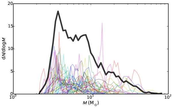
Figure 1: Pre-explosion progenitor mass posterior distributions for each of the 62 SLSNe in our sample (i.e., the ejecta mass plus a nominal neutron star mass of 1.8 M_⊙) from which we construct the joint posterior of the full sample distribution (black line). Most events have well-constrained (narrow) distributions. By combining the posteriors of each SLSN, the final summed distribution correctly reflects the uncertainty for each event.

3 Progenitor Mass Distribution

3.1 Observed Characteristics

The key outputs of the light curve models are the ejecta mass ($M_{\rm ej}$) and the neutron star’s initial spin ($P$) and magnetic field strength ($B$). To infer the progenitor masses at the time of explosion ($M$) we add a nominal neutron star remnant mass of $1.8$ M_⊙ to $M_{\rm ej}$. While the range of masses of neutron stars formed after the core collapse of massive stars in general, and SLSNe in particular, is not precisely known, existing mass measurements of Galactic neutron stars suggest a range of $\sim 1.4-2.2$ M_⊙ (e.g. for a review see Özel & Freire, 2016), making 1.8 M_⊙ a reasonable mass to use. This is consistent with the masses inferred by Nicholl et al. (2017b), who marginalized over neutron star mass as a free parameter in their fits. We stress that varying the neutron star mass at the level of a few tenths of a solar mass does not affect our conclusions.

In Figure 1 we plot the individual posterior distributions of $M$ for all 62 SLSNe in our sample. The sample spans a broad range of masses, from about 3 to 40 M_⊙. For some events the posteriors are well constrained, while for others a broader range of masses can be accommodated by the data. In the following analysis we use the combined full posterior distribution of $M$, taking into account possible degeneracies with the engine parameters and other model nuisance parameters (e.g., opacities, dust extinction).

We also plot in Figure 1 the full SLSN mass distribution, ${\rm d}N/{\rm dlog}M$, calculated by summing the mass posteriors for all 62 SLSNe. The observed mass distribution exhibits several interesting features. First, there is a sharp decline below about 3.6 M_⊙ (i.e., $M_{\rm ej}\approx 1.8$ M_⊙). As we show below, this sharp decline is not due to an observational bias, and indeed Type Ib/c SN progenitors exhibit a similar turnover in their pre-explosion mass distribution.

Second, at masses of $\approx 3.6$ to $\approx 40$ M_⊙ the distribution appears to follow a broken power law with a mild decline to about 9 M_⊙ and a sharper decline thereafter. Fitting the distribution with such a model (Figure 2), where the two power-law indices and the location of the break are free parameters, we find ${\rm d}N/{\rm dlog}M\propto M^{-0.41\pm 0.06}$ at $3.6-8.6$ M_⊙ and $\propto M^{-1.26\pm 0.06}$ at $8.6-40$ M_⊙. A single power-law fit gives an index of $-0.80\pm 0.02$ (Figure 2), but it is inferior as indicated by assessing the goodness-of-fit using a testing procedure based on the Kolmogorov-Smirnov (KS) test statistic. We find $p\lesssim 3\times 10^{-3}$, indicating that we can reject at $>3\sigma$ significance the null hypothesis that the SLSN mass distribution is drawn from the fitted single power-law distribution. Performing the same goodness-of-fit assessment for the broken power-law fit, we find $p\approx 0.16$ indicating the SLSN distribution is consistent with being drawn from a broken power-law distribution.

Finally, we find a sharp decline at $\gtrsim 40$ M_⊙, but this is likely due to the finite sample size, with the higher masses representing the tails of the posterior distributions of a few individual events (Figure 1), rather than an actual trend in the data. We do note, however, that the drop-off occurs at the core mass where mass ejections due to the pulsational pair-instability (PPI) are expected to become important (Woosley, 2017). The final explosions of stars that undergo PPI should therefore eject $\lesssim 40$ M_⊙, leading to a prediction for a drop-off in the pre-explosion mass distribution. The robustness of this drop-off will be tested with a larger sample in the future.

To assess for any redshift evolution in the SLSN mass distribution we divide the sample into low and high redshift bins using a range of redshift cuts (see Appendix). While there is a hint that the lowest redshift events ($z\lesssim 0.25$) contain fewer high mass progenitors, the sample size at these redshifts is too small ($N=23$) to make a robust statement. Using the median redshift of $z\approx 0.31$ to divide the sample, we find no significant change in the mass distribution from low to high redshift (i.e., dividing the sample by redshift is statistically consistent with dividing the sample randomly).

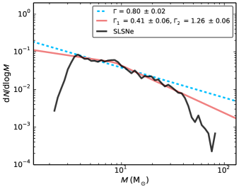
Figure 2: Pre-explosion progenitor mass distribution of SLSNe (black; from Figure 1) compared to single (dashed blue line) and broken (solid red line) power-law fits. The power-law index, $\Gamma$, defined in the equation ${\rm d}N/{\rm dlog}M\propto M^{-\Gamma}$, is given for the single power-law fit, as well as the corresponding indices, $\Gamma_{1}$ and $\Gamma_{2}$, for the broken power-law fit above and below the break mass of 8.6 M_⊙, respectively.

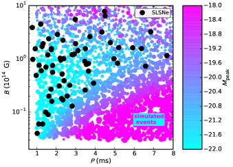
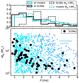
Figure 3: Top: The $B-P$ parameter space showing the wedge filled by the observed sample (black points), which corresponds to $M_{\rm peak}\lesssim-20.5$. Bottom: $M_{\rm ej}-P$ parameter space showing the parameter medians inferred for the observed sample of SLSNe (black points), as well as the parameters for the simulated models which satisfy $M_{\rm peak}<-20.5$ mag and $t_{\rm dur}>30$ days (colored points; $t_{\rm dur}$ defined in the text). We compare the projected spin histograms for the full observed (solid black) and simulated (solid cyan) samples to those for $M_{\rm ej}<3$ M_⊙ (dashed black and cyan). While the observed spin distribution summed over all masses is overall similar to that from the models, at $M_{\rm ej}<3$ M_⊙, the distribution is shifted to slower spins compared to the models.

3.2 Selection Effects

To understand how observational selection biases may affect the inferred progenitor mass distribution we simulate a grid of 3,000 magnetar-powered SLSN light curves, sampled from uniform distributions of $M_{\rm ej}$ ($1-60$ M_⊙), $P$ ($1-8$ ms), and $B$ ($0.03-10\times 10^{14}$ G). We furthermore assume a Gaussian ejecta velocity distribution with a mean and standard deviation based on observed SLSNe (Liu et al., 2017). We fix the opacity and gamma-ray opacity to 0.16 cm² g^-1 and 0.04 cm² g^-1, respectively, motivated by typical values inferred for the observed SLSN sample (Nicholl et al., 2017b). To be consistent with our nominal neutron star mass above, we fix the neutron star mass for these models at 1.8 M_⊙. For each simulated light curve we measure the peak $r$-band absolute magnitude, $M_{\rm peak}$, and the duration ($t_{\rm dur}$, defined as the timescale within 1 magnitude of peak). While simulating the complex processes by which SLSNe are identified from heterogeneous optical time-domain surveys is beyond the scope of this paper, we test the overall effect of applying simple selection criteria to the model set.

In particular, we select models with peak absolute $r$-band magnitude of $\lesssim-20.5$, chosen to match the distribution of the observed sample. As shown in Figure 3, where we plot the model events and observed SLSNe in the $B-P$ parameter space, the observed sample indeed matches models with $M_{\rm peak}\lesssim-20.5$. This selection effect leads to events that span a specific “wedge” in the $B-P$ parameter space, with a general bias against models with low $B$ values and slow spin, as well as a drop off at large values of $B\gtrsim 10^{15}$ G. This is because of the mis-match in spin-down and diffusion timescales at high $B$ and typical $E/M$ (Nicholl et al., 2017b).

We further test the effect of SLSN light curve duration, in particular that fast evolving SLSNe may be missed either due to survey cadence restrictions or to an overall shape similarity to more common SN types (Ia, Ib/c). To simulate this effect we select models with durations of $\gtrsim 30$ d, the approximate duration of a Type Ia SN. In Figure 3 we also plot the models which satisfy both the duration and luminosity cuts in $M_{\rm ej}-P$ parameter space, and compare to the observed events.

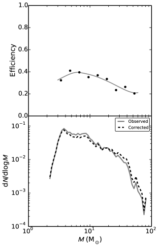
Figure 4: Top: Combined efficiency as a function of $M$ including both duration and luminosity effects calculated from our model light curves. The slight decrease at low mass is a reflection of the duration cut, while the gradual decrease at high mass reflects the peak luminosity cut. Bottom: A comparison of the observed (grey solid line) and efficiency-corrected (black dashed line) SLSN pre-explosion progenitor mass distribution.

With these simple, but observationally motivated, cuts on peak absolute magnitude and duration we assess the effect on the resulting distribution of $M$; namely, we calculate the SLSN detection efficiency as a function of $M$ by taking the ratio of the mass distribution of the model events with the cuts applied to the uniform input distribution. As shown in Figure 4 we find that the efficiency slightly varies with mass. There is a mild decrease at $\lesssim 6$ M_⊙ mainly due to resulting durations of $\lesssim 30$ d, and a gradual decrease in efficiency at higher masses due to an increasing fraction of events with peak magnitudes below $-20.5$ (apparent in the bottom panel of Figure 3). However, the overall variation in efficiency across the full mass range is less than a factor of 2.

Applying this efficiency curve as a correction factor to the observed distribution of $M$ we find that the overall effect is minor, and primarily serves to slightly flatten the broken power-law shape of the uncorrected distribution (Figure 4). Performing the same power-law fits as before, we find a single power-law index of $-0.72\pm 0.02$ (compared to $-0.80\pm 0.02$ for the uncorrected distribution), and a broken power-law fit with indices of $-0.54\pm 0.08$ and $-0.92\pm 0.05$ below and above the same break at 8.6 M_⊙ (also a free parameter), respectively. Carrying out the same Monte Carlo KS goodness-of-fit procedure to assess the single power-law fit, we find $p\approx 8\times 10^{-3}$, indicating that we can still rule out the possibility that the data are drawn from a single power law. The broken power-law model has $p\approx 0.12$.

This indicates that the broken power-law shape of the distribution is statistically robust, and not a result of the basic selection effects considered here. Therefore, the shape of the observed mass distribution can be taken to reflect the progenitor initial mass function (IMF) and subsequent stellar and binary evolution effects. In the subsequent sections we compare the observed distribution to the implied pre-supernova mass distributions from stellar and binary evolution models to determine what type of progenitors are capable of reproducing the distribution.

3.3 Comparison to Type Ib/c SNe

In Figure 5 we show a comparison of the SLSN pre-explosion mass distribution to the corresponding distribution for Type Ib/c SNe (SNe Ib/c). We use the SN Ib/c samples from Lyman et al. (2016) and Taddia et al. (2018) who provide ejecta masses from the modeling of bolometric light curves. Another recent sample from Prentice et al. (2019) is consistent with the results of these studies. We add the same nominal neutron star mass of 1.8 M_⊙ to these values to infer the pre-explosion progenitor masses. We create smooth distributions via kernel density estimation using a gaussian kernel with a bandwidth of 0.8 M_⊙, the typical uncertainty in the ejecta mass estimates. The SLSN and SN Ib/c $M$ distributions exhibit both similarities and critical differences. Both distributions exhibit a sharp decline at $\lesssim 3.5$ M_⊙ suggesting that in both cases the minimum progenitor masses are shaped by the same process, regardless of the ultimate fate of the explosion.

However, beyond the minimum cutoff the distributions differ. The bulk of SNe Ib/c have pre-explosion progenitors in the range $M\approx 3-5$ M_⊙. There are essentially no SN Ib/c progenitors with masses of $\gtrsim 10$ M_⊙, while SLSN progenitors extend to $\approx 40$ M_⊙. In addition, between 3.5 and 10 M_⊙ the SN Ib/c distribution follows a much steeper (and single) power-law decline, ${\rm d}N/{\rm dlog}M\propto M^{-2.8}$, than the SLSN progenitors over this mass range (or in fact their entire mass range).

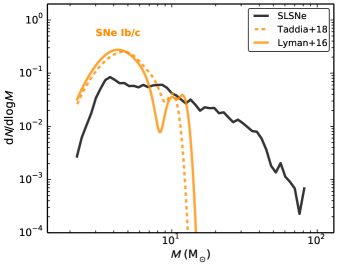
Figure 5: The pre-explosion mass distribution of SLSNe (black) compared to that for Type Ib/c SNe (solid orange: Lyman et al. 2016; dashed orange: Taddia et al. 2018).

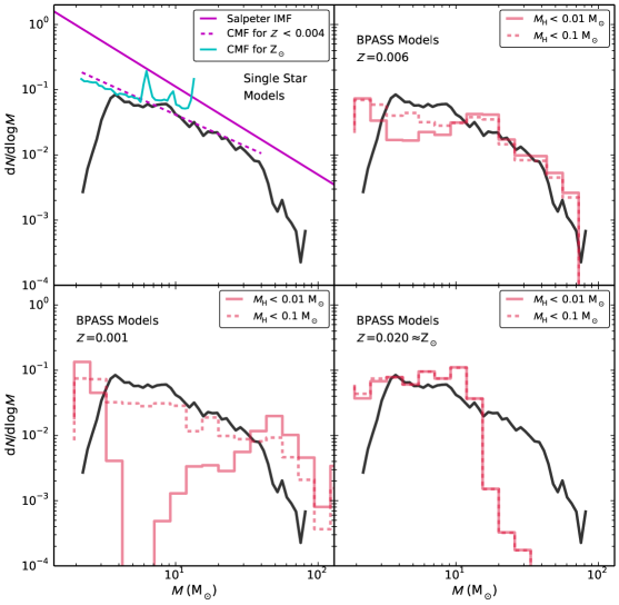
Figure 6: SLSN pre-explosion mass distribution (black line) compared to the distributions of CO core masses (CMFs) calculated using $M_{\rm ZAMS}-M_{\rm CO}$ relations from single star models (top left) at metallicities of $Z_{\odot}$ (solid cyan) and $Z<0.004$ (dashed magenta) and the distributions of final primary star masses from BPASS binary star models for metallicities of $Z=0.006$ (top right), $Z=0.001$ (bottom left), and $Z=0.020$ (bottom right). We show the BPASS distributions for two cuts on the remaining hydrogen mass: $M_{\rm H}<0.01$ M_⊙ and $M_{\rm H}<0.1$ M_⊙. For reference we also show the Salpeter IMF (solid magenta) in the top left panel.

3.4 Comparison to Single Star Model Mass Functions

To understand the physics encoded by the shape of the pre-explosion progenitor mass distribution of SLSNe, we compare the distribution with the IMF, which for most variations follows the Salpeter power-law slope at high masses (Salpeter, 1955):

$$\frac{{\rm d}N}{{\rm dlog}M}\propto M^{-1.35}.$$ (1)

As shown in Figure 6, the IMF matches well with the slope of the observed SLSN mass distribution at $\gtrsim 9$ M_⊙, but there is a clear deficit in the observed mass distribution at lower masses compared to the IMF expectation.

Since the IMF provides the distribution of zero-age main sequence (ZAMS) masses, while the pre-explosion mass distribution of SLSNe reflects significant mass loss and stripping, a more relevant comparison is to the core mass function (CMF). Stellar evolution models indicate a dependence between ZAMS mass, core mass, and metallicity, which in turn influences mass loss.

We first compare the SLSN distribution with the expected CMF from stellar evolution models of solar metallicity stars, which experience significant mass loss due to line-driven winds. We use models from Sukhbold et al. (2016), which extend to ZAMS masses of 120 M_⊙. The relation between core mass ($M_{\rm CO}$) and $M_{\rm ZAMS}$ for these models is a power law up to $M_{\rm ZAMS}\approx 40$ M_⊙ where $M_{\rm CO}$ peaks around 14 M_⊙. Beyond $M_{\rm ZAMS}\approx 40$ M_⊙ the relation turns over and lower mass cores are produced due to increased mass loss. In Figure 6 we show the resulting CMF for solar metallicity stars, which exhibits a relatively flat shape, with peaks caused by broad ranges of $M_{\rm ZAMS}$ that produce similar values of $M_{\rm CO}$, and an upper bound of about 14 M_⊙. The CMF for solar metallicity stars is therefore not a good match to the SLSN distribution. Solar metallicity models from Spera et al. (2015) are similarly unable to produce core masses of $\gtrsim 20$ $M_{\odot}$. The fact that solar metallicity models cannot explain the SLSN mass distribution is consistent with the observed preference of SLSNe in low metallicity ($Z\lesssim 0.4$ Z_⊙) host galaxies (Chen et al., 2013; Lunnan et al., 2014; Leloudas et al., 2015; Perley et al., 2016; Schulze et al., 2018).

We next investigate low metallicity single star models. Low metallicity stars generally lose less mass over their lifetimes and therefore yield CO core masses that increase monotonically with ZAMS mass. Using the models of Sukhbold et al. (2018) with the lowest mass-loss rates (appropriate for low metallicity) we find that the relation between $M_{\rm CO}$ and $M_{\rm ZAMS}$ is a power law:

$$M_{\rm CO}\propto M_{\rm ZAMS}^{1.37}.$$ (2)

A similar relation is obtained for the low metallicity models ($Z<0.004$) in Spera et al. (2015), determined using a different stellar evolution code. Combined with a Salpeter IMF this gives:

$$\frac{{\rm d}N}{{\rm dlog}M}\propto M_{\rm CO}^{-0.99}.$$ (3)

In Figure 6 we plot the low metallicity CMF (truncated at the approximate core mass of $M\sim 40$ M_⊙ where the PPI is expected to become strong; Woosley 2017) which exhibits much better agreement with the SLSN mass distribution. Although in detail it does not strictly provide a broken power law shape that is preferred by the data. A key caveat of this comparison, however, is that the low metallicity models that yield this CMF predict that the stars will retain much of their hydrogen envelope at the time of explosion, whereas SLSN progenitors have been stripped of their envelopes.

In summary, for single star models, only low metallicity stars can generally account for the full range of pre-explosion (CO core) masses observed for SLSNe, as well as roughly the overall shape of the progenitor mass distribution. However, the single star low metallicity models retain a significant hydrogen envelope at the time of explosion, making them incompatible with SLSN progenitors. Recently Woosley (2019) explored the evolution of hydrogen-poor stars using models of helium stars that have already lost their hydrogen envelopes. Subsequent mass-loss was modeled assuming solar metallicity. The resulting relation between the pre-supernova mass and $M_{\rm ZAMS}$ is similar in form to Equation 3 (their Equations 13 and 14), but with masses that are about half of $M_{\rm CO}$ in single star models with a hydrogen envelope. Thus, in the Woosley (2019) models explaining pre-explosion SLSN progenitors with $\gtrsim 20$ M_⊙ requires initial helium stars with $M_{\rm He}\gtrsim 40$ M_⊙ (corresponding to ZAMS masses $\gtrsim 80$ M_⊙). Importantly, this relation is also unable to account for the broken power law shape of the observed SLSN mass distribution. At low metallicity, and therefore lower mass-loss rates, less massive helium stars are needed to explain such massive pre-explosion cores. A $Z=0$ helium star with an initial mass of 30 M_⊙ modelled in Woosley (2017) yielded a CO core mass of $\approx 25$ M_⊙.

A key ingredient of the magnetar model for SLSNe is rapid rotation. None of the models discussed above include the effects of rotation on the late evolution. Recently Aguilera-Dena et al. (2018) explored the evolution of rapidly rotating stars, including models with enhanced rotational mixing that experience chemically homogeneous evolution (CHE) and leave behind relatively bare CO cores, potentially relevant for SLSNe. We find that the relation between $M_{\rm CO}$ and $M_{\rm ZAMS}$ implied by their models is also nearly linear, although these models produce larger CO core masses for a given $M_{\rm ZAMS}$ than the non-rotating models, which is in agreement with other models of rapidly rotating stars (e.g., Yoon et al. 2006; Chatzopoulos & Wheeler 2012; Woosley 2017). This means that less massive initial stars are required to produce pre-explosion progenitors in the mass range observed for SLSNe. For example, their model with an initial mass of 39 M_⊙ yields a final mass of $\approx 22$ M_⊙, whereas non-rotating models required $\approx 80$ M_⊙ to produce such massive cores. While these models are promising for SLSNe, the mass “resolution” of the implied relation from these models (they present models at only 6 specific masses) is not sufficient for a robust comparison with the detailed shape of the observed distribution.

3.5 Comparison to Binary Star Models

Another proposed mechanism for producing a bare CO core while maintaining rapid rotation is through interaction in a binary system. It has long been suspected that binary interactions may be the dominant mechanism by which normal stripped SNe lose their hydrogen envelopes (e.g., Podsiadlowski et al., 1992), and the ejecta mass distributions of normal SNe Ib/c have been argued to be consistent with predictions from binary star models (Lyman et al., 2016). In Figure 6 we compare our observed SLSN progenitor mass distribution with mass distributions from models of binary stars. We use models of primary stars from the Binary Population and Spectral Synthesis (BPASS) suite of binary evolution models (Version 2.2; Eldridge et al., 2017; Stanway, & Eldridge, 2018). In particular we use the “z001”, “z006”, and “z020” models, which are calculated for metallicities of $Z=0.001$ ($\approx 1/20$ Z_⊙), $Z=0.006$ ($\approx 1/3$ Z_⊙), and $Z=0.020$ ($\approx$ Z_⊙), respectively. We select those models that have remaining hydrogen masses of $M_{\rm H}<10^{-2}$ M_⊙ to restrict to models that produce stripped-envelope progenitors. In Figure 6 we show the distributions of final primary star masses, weighted by an input Salpeter IMF, at each metallicity. We also show the equivalent distributions for a relaxed cut on remaining hydrogen of $M_{\rm H}<10^{-1}$ M_⊙ to understand its effect on the distributions.

We find that the resulting distribution for $Z=0.006$ matches the observed SLSN mass distribution relatively well at $\gtrsim 10$ M_⊙, and also exhibits a flattening at lower masses as seen in the data, but with a significant deficit in expected numbers compared to the data that depends on the cut on $M_{\rm H}$. The BPASS model distribution of stripped primary stars extends to the highest progenitor masses we find for SLSNe. At a lower metallicity of $Z=0.001$ we find a gap between two populations of stripped ($M_{\rm H}<10^{-2}$ M_⊙) stars at $M\sim 2-3$ M_⊙ and $M\gtrsim 10$ M_⊙, in stark contrast to the observed SLSN distribution, likely an indication that the low mass loss rates at these metallicities prevent the formation of stripped progenitors in the range $M\sim 3-10$ M_⊙. The solar metallicity models yield pre-explosion progenitors which span a similar range as the solar metallicity single star models, including a similarly steep drop-off at $M\gtrsim 10$ M_⊙. Therefore, among the three metallicities considered, the $Z=0.006$ models (representative of measured SLSN host galaxy metallicities) are best able to reproduce the observed SLSN distribution. While the $Z=0.006$ distribution of stripped primary stars extends to the highest progenitor masses we find for SLSNe, the ability of the resulting explosions to actually eject most of the mass depends on the SN kinetic energy.

Figure 7: Ejecta mass distribution (i.e., calculated without adding the nominal remnant mass to each event) of our SLSN sample (solid black) compared to the ejecta masses from stripped primary star progenitors from BPASS models at metallicity $Z=0.006$. The model ejecta masses are calculated for both a kinetic energy of 10⁵¹ erg (dashed orange) and 10⁵² erg (solid cyan).

To explore this effect, in Figure 7 we directly compare the distribution of $M_{\rm ej}$ for SLSNe with BPASS models at $Z=0.006$ calculated for SN kinetic energies of $10^{51}$ and $10^{52}$ erg. We find that the ejecta masses in the $10^{51}$ erg models rapidly drop off at $\approx 8$ M_⊙. However, the $10^{52}$ erg models lead to the large ejecta masses seen in the observed SLSN distribution. This therefore indicates that if SLSN progenitors evolve via a binary channel similar to the BPASS models, then a significant fraction of the events require much larger explosion energies than for normal SNe. The magnetar models generally predict large kinetic energies with a median near $5\times 10^{51}$ erg, and many events with energies reaching $\sim 10^{52}$ erg. This is due to conversion of the magnetar spin-down energy to ejecta kinetic energy.

4 Mass-Spin Correlation

In §3.2 we explored the impact of observational selection biases on the observed pre-explosion mass distribution by analyzing the luminosity and duration of a grid of simulated magnetar light curves in relation to the observed properties of SLSNe. While these selection effects have minor impact on the mass distribution, they help us to uncover an interesting trend between $M_{\rm ej}$ and $P$ in the observed sample that is not present in the simulated light curves. In Figure 3 we plot the observed and simulated events in the parameter space of $M_{\rm ej}$ and $P$, after removing simulated events with a low peak brightness of $\gtrsim-20.5$ mag and a short duration of $\lesssim 30$ d. In the observed sample we find an overall correlation between $M_{\rm ej}$ and $P$, such that events with rapid spin tend to have higher ejecta masses than those with slower initial spin. In particular, we find a dearth of SLSNe with $M_{\rm ej}\lesssim 3$ M_⊙ and $P\lesssim 3$ ms. Conversely, we find that nearly all events with $M_{\rm ej}\gtrsim 8$ M_⊙ have $P\lesssim 3$ ms.

A comparison to the simulated events, after accounting for the main observational selection effects, indicates that the paucity of observed SLSNe with large $M_{\rm ej}$ and slow $P$ is at least partly due to an observational selection effect since these events tend to have systematically lower peak luminosities (Figure 3). On the other hand, the lack of observed SLSNe with low $M_{\rm ej}$ and fast $P$ cannot be explained as an observational bias, with a significant fraction of the simulated events residing in this corner of parameter space.

In Figure 8 we show sample model light curves for events with $M_{\rm ej}\approx 1.5$ M_⊙ and $P\approx 1.5$ ms for a wide range of magnetic field strengths. Most of these events have high peak luminosities and sufficiently long durations to be captured in optical sky surveys. We therefore conclude that the lack of observed SLSNe with $M_{\rm ej}\lesssim 3$ M_⊙ and $P\lesssim 3$ ms is a real physical effect, and not an observational bias.

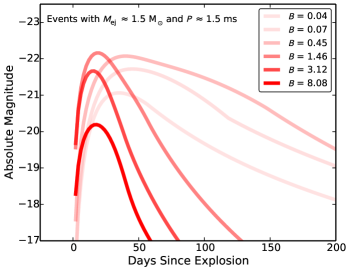
Figure 8: Model $r$-band light curves from the region of parameter space with low $M_{\rm ej}$ and low $P$, showing the effect of magnetic field strength on duration ($B$ is given in units of 10¹⁴ G). While some events in this region evolve rapidly and may be missed by surveys, most are of sufficient duration to be captured. Therefore the lack of observed events in this region of parameter space is not simply the result of an observational bias.

We simulate two possible effects to test whether they can account for this: (i) removing low ejecta mass ($\lesssim 3$ M_⊙) events with $P<3$ ms from the simulated set, and (ii) systematically shifting such model events to slower spins (implemented by randomly shifting their spins to the range $P=3-4.5$ ms). These effects are designed to explore the possibilities that low mass progenitors with rapid spin are either not produced, or that they are spun down by $\approx 1-2$ ms. In Figure 9 we compare the cumulative spin distributions for the observed and simulated SLSNe with $M_{\rm ej}\lesssim 3$ M_⊙, which are significantly different as already hinted at above. As shown in the Figure, the resulting simulated distribution after shifting model events to slower spins provides a better match to the observed sample than the distribution after completely removing them from the sample.

This simple exercise lends support to the idea that the correlation between $M_{\rm ej}$ and $P$ is not simply the result of events being missed by surveys. While we lack a detailed physical model that might explain this correlation, the effect of shifting events to slower spins could potentially be physically motivated by a process in which angular momentum is removed due to mass loss. The lowest mass SLSN pre-explosion progenitors may be stars which have undergone enhanced mass loss relative to their more massive counterparts, leading to slower remnant spins.

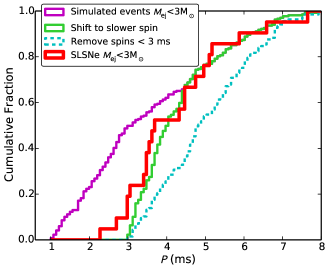
Figure 9: Cumulative $P$ distributions for the models (with duration and luminosity cuts applied) and observed sample at $M_{\rm ej}<3$ M_⊙, showing the significant difference at low $P$. We also show distributions of the models after shifting models with $P<3$ ms to slower spins or removing them completely from the model set.

5 Discussion and Implications

In §3.1 we found that the pre-explosion progenitor mass distribution of SLSNe exhibits a steep decline at $M\lesssim 3.6$ M_⊙ and a broken power-law shape with indices of $-0.41$ at $3.6$ M_⊙ $<M<8.6$ M_⊙ and $-1.26$ at $8.6$ M_⊙ $<M<40$ M_⊙. While the broad shape is similar to the expected shape of the $M_{\rm CO}$ distribution (assuming an initial population following the Salpeter IMF) implied by models with fine mass grids of non-rotating low-metallicity single massive stars, as well as models of non-rotating helium stars, none of the non-rotating single star stellar models we explored provide a clear prediction that matches the detailed shape of the observed distribution. This is consistent with the expected importance of rapid rotation.

Confirming initial conclusions from a smaller sample (Nicholl et al., 2015b), our comparison with SNe Ib/c shows that while many SLSNe result from progenitors of similar masses as SNe Ib/c, a significant fraction of SLSNe originate from progenitors with $M\gtrsim 10$ M_⊙ and are therefore much more massive than a typical SN Ib/c progenitor. Our larger sample provides further insight. Namely, the power law shape of the distributions where they do overlap is different, with SNe Ib/c following a steeper slope than SLSNe. These observations are a robust indication that the progenitors of SNe Ib/c and SLSNe exhibit different properties which impact the mass of stars that can explode. These properties are likely related to the different evolutionary pathways (e.g., due to rapid rotation at low metallicity) which enable the production of a magnetar capable of enhancing the radiative output.

The BPASS models suggest that achieving a SN with $M_{\rm ej}\gtrsim 8-10$ M_⊙ requires a large kinetic energy, which may only be possible if a magnetar is formed. This comes from a binding energy argument for the primary star, and is thus not strictly a consequence of its prior binary evolution. Otherwise, assuming a canonical explosion energy of $\sim 10^{51}$ erg, core-collapses of such massive stars do not have enough energy to unbind most of their mass, leading to the formation of black holes (Heger et al., 2003) and possibly fallback accretion powered SNe (Dexter & Kasen, 2013). The presence of a magnetar in SLSNe is therefore consistent with the broadening of the mass distribution relative to SNe Ib/c as the extra kinetic energy provided by the spin-down power allows for a more massive star to explode. To summarize, the broad mass distribution that we observe for SLSNe is evidence that rotational energy is capable of not only enhancing the radiative output of a SN, but also the mass range of stars which can actually explode. This is in contrast to the CSM interaction model for SLSNe, in which only the efficiency with which the available energy is converted to radiation is increased.

Within the stripped-envelope SN class, SLSNe appear to be most similar to SNe Ic-BL in their mean spectroscopic (Liu et al., 2017; Nicholl et al., 2019) and host environment properties (Lunnan et al., 2014). In addition, several direct links have been found, including the SLSN SN 2017dwh which evolved from a blue SLSN-like spectrum (with unusually strong absorption from Co II) to appear nearly identical to SNe Ic-BL (Blanchard et al., 2019). Also, the luminous ($M\approx-20$ mag) SN 2011kl was found to be associated with the ultra-long GRB 111209A (Greiner et al., 2015). While SN 2011kl was bluer and relatively featureless compared to previous SNe Ic-BL known to be associated with LGRBs, its discovery suggested a possible continuum of behavior from SNe Ic-BL to SLSNe with the implication being that these transients are linked by a common central engine mechanism (Kann et al., 2019).

It is therefore of particular interest to compare the pre-explosion progenitor masses of SLSNe with those of SNe Ic-BL. While a similarly detailed distribution for SNe Ic-BL does not yet exist, light curve and spectroscopic analyses suggest on average masses higher than normal Type Ic SNe (Drout et al., 2011; Lyman et al., 2016; Prentice et al., 2019). Estimates based on spectroscopic models for SNe Ic-BL associated with LGRBs are generally at the high mass end (e.g., $\approx$ 10 M_⊙ for SN 1998bw, SN 2003lw, and SN 2003dh; Iwamoto et al. 1998; Mazzali et al. 2013), similar to many SLSNe. This combined with the insight from events like SN 2017dwh, nebular spectra, and environmental comparisons, suggests that the progenitor pathways which produce SLSNe are more similar to those that produce LGRBs and their associated SNe Ic-BL than those that produce normal SNe Ib/c.

5.1 Shape of the Mass Distribution as a Clue for Progenitor Formation

Evolutionary models of non-rotating low metallicity stars generically predict a power-law relationship between $M_{\rm CO}$ and $M_{\rm ZAMS}$, which leads to a power-law distribution of $M_{\rm CO}$. Interestingly, our single power-law fit to the SLSN pre-explosion mass distribution gives a slope similar to the expectation for non-rotating low-metallicity stars. However, we find that a broken power law is a better description of the SLSN distribution, indicating a deviation from the simple $M_{\rm CO}$ distribution. This suggests that rotation and mass-loss processes significantly affect the distribution of pre-SN CO core masses.

In the context of a magnetar engine, rapidly rotating CO cores appear to be essential. Mass-loss and spin-up processes resulting from binary interactions (de Mink et al., 2013) as well as rotationally-induced mixing associated with CHE (Yoon & Langer, 2005; Woosley & Heger, 2006) have been proposed to explain how mostly bare rapidly rotating CO cores can be produced. In addition, some progenitors may undergo additional mass loss which removes mass from the CO cores. Recent models of such stars, produced via CHE, suggest that spin up from core contraction induces mass loss (Aguilera-Dena et al., 2018). These authors suggest that possible signatures of CSM interaction seen in several SLSNe (e.g., light curve bumps; Nicholl et al. 2016a; Inserra et al. 2017; Yan et al. 2017; Blanchard et al. 2018) is evidence of this mass-loss process and that it may occur regardless of how rapidly rotating CO stars are formed. Mass loss is therefore a key factor which influences the shape of the pre-explosion SLSN progenitor mass distribution.

Additional effects due to binary interaction are likely given that observations suggest about 70% of O stars experience mass transfer with a binary companion (Sana et al., 2012). Woosley (2019) approximated the effects of binary interaction by studying the evolution of helium stars which have already lost their hydrogen envelope. However, we find that these models still predict a smooth distribution of $M_{\rm CO}$. Moreover, this study does not account for the effects of rotation and only incorporates further mass loss due to stellar winds at solar metallicity. We also compare our distribution to BPASS binary models which simultaneously take into account the effects of stellar winds, mixing due to rotation, Roche lobe overflow, and common envelope evolution. We find the mass distribution of stripped primary stars at $Z\approx 1/3$ Z_⊙ is relatively flat (in ${\rm dlog}M$) at $\lesssim 20$ M_⊙, similar to the break structure we find for SLSNe though with a higher break mass. Also, there is a relative deficit at low masses compared to the observed distribution that is sensitive to the amount of remaining hydrogen. As with single stars, the BPASS distribution strongly depends on metallicity. We show that distributions corresponding to metallicities substantially higher and lower than SLSN host galaxies provide poor matches to the SLSN distribution.

5.2 Angular Momentum Transport Weakens the Engine?

In addition to the complex shape of the pre-SN mass distribution itself, we find a trend between the pre-SN masses and the magnetar initial spin periods; SLSNe with lower ejecta masses exhibit systematically slower initial spins. This confirms initial indications of such a trend from the modeling of a smaller sample of bolometric light curves by Yu et al. (2017). Our analysis verifies this trend is not due to observational biases and suggests that the lowest mass pre-explosion progenitors are spun down, possibly a signature of significant mass loss. Though the observed trend is likely the result of multiple mechanisms, including spin up processes, acting at different stages of evolution through core collapse.

The process by which sufficient angular momentum is retained in stellar cores, in this case to form magnetars with $P\sim 1-8$ ms, is not well understood. Early models of massive single stars at solar metallicity exploring angular momentum transport effects due to magnetic torques predict initial spins of $P\gtrsim 10$ ms (Heger et al., 2005), whereas more recent models including additional instabilities predict much slower spins ($P\sim 50-200$ ms; Ma & Fuller 2019), indicating that spin up due to mass transfer or tidal effects in binary systems may play an important role (van den Heuvel & Yoon, 2007; de Mink et al., 2013). In addition, CHE at low metallicity may be key for the production of rapidly rotating remnants (Yoon & Langer, 2005).

The Aguilera-Dena et al. (2018) models of rapidly rotating CO cores predict a trend between mass and specific angular momentum of the core. Specifically, the more massive models exhibit less angular momentum transport from the core to the surface, whereas lower mass models transfer significant core angular momentum leading to slower remnant spins. In Figure 10 we plot the ejecta masses and remnant spins for the Aguilera-Dena et al. (2018) models (they assume a 1.5 M_⊙ neutron star remnant), showing this trend exhibits broad agreement with the observed SLSN mass-spin trend.

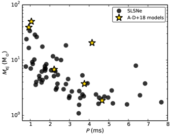
Figure 10: Comparison in $M_{\rm ej}-P$ parameter space between SLSNe (black points) and the models of Aguilera-Dena et al. (2018) of rapidly rotating stars which leave bare CO cores due to CHE (gold stars). In general, models with lower ejecta masses have slower spins, broadly consistent with the trend seen in the SLSN sample.

5.3 The Black Hole Formation Threshold

A key issue with all of the models discussed here is the threshold between neutron star and black hole formation. Although a given progenitor evolution model may predict a final pre-SN mass distribution similar to the observed SLSN pre-explosion mass distribution, whether the further evolution through core collapse produces a black hole or a neutron star is not well understood. Fallback accretion onto a black hole as an alternative central engine model for SLSNe (Dexter & Kasen, 2013) is not expected to account for the observed durations and luminosities (Moriya et al., 2018). Modeling by Ertl et al. (2019) of the explosions of helium stars from Woosley (2019) suggest that pre-SN stars with masses above 12 M_⊙ produce black holes. The resulting conflict between single star evolution models and the magnetar model given the observation of SLSNe with pre-SN masses extending to $\approx 40$ M_⊙, may be an indication that rapid rotation and additional effects from interactions in a binary system have a significant effect on black hole formation and the mass range where PPI becomes important. As discussed above, rotational energy may couple to the kinetic energy of the SN, enabling more massive stars to explode. An additional possibility is that a star that undergoes PPI may later produce a magnetar-powered SLSN, a scenario possibly supported by evidence of detached CSM shells around some SLSNe (Yan et al., 2017; Lunnan et al., 2018b). This scenario may be less and less likely as PPI effects become stronger with increasing mass, potentially reflected by the steep drop-off in the SLSN mass distribution at $M\gtrsim 40$ M_⊙.

6 Summary and Conclusions

We presented an analysis of the pre-explosion progenitor mass distribution of 62 SLSNe inferred from light curve modeling in the context of a magnetar central engine. We additionally explored possible observational biases that affect the observed mass distribution, and explored correlations between the progenitor mass and central engine properties. Our key findings are:

• The pre-explosion progenitor mass distribution spans a broad range of masses from $M\approx 3.6$ M_⊙ to $M\approx 40$ M_⊙, with steep drop-offs at both ends of the distribution, and evidence for a break at $\approx 9$ M_⊙.

• The mass distribution is best fit with a broken power law with indices of $-0.41\pm 0.06$ at $3.6-8.6$ M_⊙ and $-1.26\pm 0.06$ at $8.6-40$ M_⊙.

• While there is some variation in the observational efficiency of recognizing SLSNe as a function of progenitor and engine parameters, we find that this effect is mild and does not alter the broken power-law shape of the mass distribution.

• The SLSN mass distribution extends to much higher masses than that of SNe Ib/c ($\approx 40$ M_⊙ versus $\approx 10$ M_⊙, respectively), and also exhibits a different power-law slope in the overlapping mass range. However, both distributions exhibit a steep decline at $\lesssim 3.5$ M_⊙.

• There is a correlation between $M_{\rm ej}$ and $P$ such that events with low $M_{\rm ej}$ have systematically slower spins. Our analysis suggests these events are spun down.

This analysis provides the most detailed look to date at the pre-explosion progenitor masses of SLSNe, a key property encoding information about the evolutionary history of the progenitor stars. We further compared the pre-explosion progenitor mass distribution of SLSNe with both single and binary stellar evolution models and found the final mass distribution from models of stripped binary stars also show a break structure, whereas models of single stars do not easily explain the SLSN mass distribution.

The statistically robust break structure in the distribution and the trend between $M_{\rm ej}$ and $P$ are likely a direct result of the physical processes associated with producing a magnetar capable of enhancing the radiative output of a SN. Non-rotating single-star models do not naturally predict such trends, whereas models of rapidly rotating stars as well as evolutionary models incorporating the effects of binary interaction may. Our findings therefore demonstrate self-consistency of the magnetar central engine model for SLSNe.

Independent of model comparisons, our analysis shows that the progenitors of SLSNe differ from normal stripped-envelope SNe; the effects of rotation perhaps being the key factor determining whether a stripped star explodes as a SN Ib/c, a SLSN, or at high mass, undergo direct collapse to a black hole or produce a fallback accretion powered SN. The presence of a magnetar may naturally explain the relatively large fraction of SLSNe with massive ($M\gtrsim 10$ M_⊙) pre-explosion progenitors if the conversion of rotational energy into kinetic energy enables more massive stars to explode.

Appendix A Testing for Redshift Evolution of the Mass Distribution

In Figure 11 we show the SLSN pre-explosion progenitor mass distribution constructed from sub-samples of SLSNe divided at various redshifts.

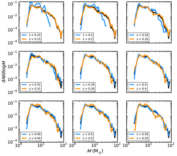
Figure 11: SLSN pre-explosion progenitor mass distribution calculated for low and high redshift sub-samples using nine different redshift cuts from $z=0.15-0.55$. The median redshift of the sample is $z\approx 0.31$. We find that dividing the sample by redshift is statistically consistent with dividing the sample randomly; in other words, we cannot discern any significant difference in the distribution at low and high redshift.

References

- Aguilera-Dena et al. (2018) Aguilera-Dena, D. R., Langer, N., Moriya, T. J., et al. 2018, ApJ, 858, 115
- Angus et al. (2019) Angus, C. R., Smith, M., Sullivan, M., et al. 2019, MNRAS, 487, 2215
- Barbary et al. (2009) Barbary, K., Dawson, K. S., Tokita, K., et al. 2009, ApJ, 690, 1358
- Berger et al. (2012) Berger, E., Chornock, R., Lunnan, R., et al. 2012, ApJ, 755, L29
- Blanchard et al. (2018) Blanchard, P. K., Nicholl, M., Berger, E., et al. 2018, ApJ, 865, 9
- Blanchard et al. (2019) Blanchard, P. K., Nicholl, M., Berger, E., et al. 2019, ApJ, 872, 90
- Chatzopoulos & Wheeler (2012) Chatzopoulos, E., & Wheeler, J. C. 2012, ApJ, 748, 42
- Chatzopoulos et al. (2013) Chatzopoulos, E., Wheeler, J. C., Vinko, J., et al. 2013, ApJ, 773, 76
- Chen et al. (2013) Chen, T.-W., Smartt, S. J., Bresolin, F., et al. 2013, ApJ, 763, L28
- Chen et al. (2015) Chen, T.-W., Smartt, S. J., Jerkstrand, A., et al. 2015, MNRAS, 452, 1567
- Chen et al. (2017) Chen, T.-W., Nicholl, M., Smartt, S. J., et al. 2017, A&A, 602, A9
- Chevalier & Irwin (2011) Chevalier, R. A. & Irwin, C. M. 2011, ApJ, 729, L6
- Chomiuk et al. (2011) Chomiuk, L., Chornock, R., Soderberg, A. M., et al. 2011, ApJ, 743, 114
- De Cia et al. (2018) De Cia, A., Gal-Yam, A., Rubin, A., et al. 2018, ApJ, 860, 100
- de Mink et al. (2013) de Mink, S. E., Langer, N., Izzard, R. G., et al. 2013, ApJ, 764, 166
- Dessart et al. (2012) Dessart, L., Hillier, D. J., Waldman, R., et al. 2012, MNRAS, 426, L76
- Dexter & Kasen (2013) Dexter, J., & Kasen, D. 2013, ApJ, 772, 30
- Drout et al. (2011) Drout, M. R., Soderberg, A. M., Gal-Yam, A., et al. 2011, ApJ, 741, 97
- Eftekhari et al. (2019) Eftekhari, T., Berger, E., Margalit, B., et al. 2019, ApJ, 876, L10
- Eldridge et al. (2017) Eldridge, J. J., Stanway, E. R., Xiao, L., et al. 2017, PASA, 34, e058
- Ertl et al. (2019) Ertl, T., Woosley, S. E., Sukhbold, T., et al. 2019, arXiv e-prints, arXiv:1910.01641
- Gal-Yam et al. (2009) Gal-Yam, A., Mazzali, P., Ofek, E. O., et al. 2009, Nature, 462, 624
- Gal-Yam (2012) Gal-Yam, A. 2012, Science, 337, 927
- Gomez et al. (2019) Gomez, S., Berger, E., Nicholl, M., et al. 2019, ApJ, 881, 87
- Greiner et al. (2015) Greiner, J., Mazzali, P. A., Kann, D. A., et al. 2015, Nature, 523, 189
- Guillochon et al. (2017) Guillochon, J., Parrent, J., Kelley, L. Z., et al. 2017, ApJ, 835, 64
- Guillochon et al. (2018) Guillochon, J., Nicholl, M., Villar, V. A., et al. 2018, The Astrophysical Journal Supplement Series, 236, 6
- Heger & Woosley (2002) Heger, A. & Woosley, S. E. 2002, ApJ, 567, 532
- Heger et al. (2003) Heger, A., Fryer, C. L., Woosley, S. E., et al. 2003, ApJ, 591, 288
- Heger et al. (2005) Heger, A., Woosley, S. E., & Spruit, H. C. 2005, ApJ, 626, 350
- Howell et al. (2013) Howell, D. A., Kasen, D., Lidman, C., et al. 2013, ApJ, 779, 98
- Inserra et al. (2013) Inserra, C., Smartt, S. J., Jerkstrand, A., et al. 2013, ApJ, 770, 128
- Inserra et al. (2017) Inserra, C., Nicholl, M., Chen, T.-W., et al. 2017, MNRAS, 468, 4642
- Iwamoto et al. (1998) Iwamoto, K., Mazzali, P. A., Nomoto, K., et al. 1998, Nature, 395, 672
- Jerkstrand et al. (2016) Jerkstrand, A., Smartt, S. J. & Heger, A. 2016, MNRAS, 455, 3207
- Jerkstrand et al. (2017) Jerkstrand, A., Smartt, S. J., Inserra, C., et al. 2017, ApJ, 835, 13
- Kann et al. (2019) Kann, D. A., Schady, P., Olivares E., F., et al. 2019, A&A, 624, A143
- Kasen & Bildsten (2010) Kasen, D., & Bildsten, L. 2010, ApJ, 717, 245
- Leloudas et al. (2012) Leloudas, G., Chatzopoulos, E., Dilday, B., et al. 2012, A&A, 541, A129
- Leloudas et al. (2015) Leloudas, G., Schulze, S., Krühler, T., et al. 2015, MNRAS, 449, 917
- Liu et al. (2017) Liu, Y.-Q., Modjaz, M., & Bianco, F. B. 2017, ApJ, 845, 85
- Liu et al. (2017) Liu, L.-D., Wang, S.-Q., Wang, L.-J., et al. 2017, ApJ, 842, 26
- Lunnan et al. (2013) Lunnan, R., Chornock, R., Berger, E., et al. 2013, ApJ, 771, 97
- Lunnan et al. (2014) Lunnan, R., Chornock, R., Berger, E., et al. 2014, ApJ, 787, 138
- Lunnan et al. (2016) Lunnan, R., Chornock, R., Berger, E., et al. 2016, ApJ, 831, 144
- Lunnan et al. (2018a) Lunnan, R., Chornock, R., Berger, E., et al. 2018a, ApJ, 852, 81
- Lunnan et al. (2018b) Lunnan, R., Fransson, C., Vreeswijk, P. M., et al. 2018b, Nature Astronomy, 2, 887
- Lunnan et al. (2019) Lunnan, R., Yan, L., Perley, D. A., et al. 2019, arXiv e-prints, arXiv:1910.02968
- Lyman et al. (2016) Lyman, J. D., Bersier, D., James, P. A., et al. 2016, MNRAS, 457, 328
- Ma & Fuller (2019) Ma, L., & Fuller, J. 2019, MNRAS, 488, 4338
- Mazzali et al. (2013) Mazzali, P. A., Walker, E. S., Pian, E., et al. 2013, MNRAS, 432, 2463
- Mazzali et al. (2016) Mazzali, P. A., Sullivan, M., Pian, E., et al. 2016, MNRAS, 458, 3455
- McCrum et al. (2014) McCrum, M., Smartt, S. J., Kotak, R., et al. 2014, MNRAS, 437, 656
- McCrum et al. (2015) McCrum, M., Smartt, S. J., Rest, A., et al. 2015, MNRAS, 448, 1206
- Milisavljevic et al. (2013) Milisavljevic, D., Soderberg, A. M., Margutti, R., et al. 2013, ApJ, 770, L38
- Moriya et al. (2018) Moriya, T. J., Nicholl, M., & Guillochon, J. 2018, ApJ, 867, 113
- Nicholl et al. (2013) Nicholl, M., Smartt, S. J., Jerkstrand, A., et al. 2013, Nature, 502, 346
- Nicholl et al. (2014) Nicholl, M., Smartt, S. J., Jerkstrand, A., et al. 2014, MNRAS, 444, 2096
- Nicholl et al. (2015a) Nicholl, M., Smartt, S. J., Jerkstrand, A., et al. 2015a, ApJ, 807, L18
- Nicholl et al. (2015b) Nicholl, M., Smartt, S. J., Jerkstrand, A., et al. 2015b, MNRAS, 452, 3869
- Nicholl, & Smartt (2016) Nicholl, M., & Smartt, S. J. 2016, MNRAS, 457, L79
- Nicholl et al. (2016a) Nicholl, M., Berger, E., Smartt, S. J., et al. 2016a, ApJ, 826, 39
- Nicholl et al. (2016b) Nicholl, M., Berger, E., Margutti, R., et al. 2016b, ApJ, 828, L18
- Nicholl et al. (2017a) Nicholl, M., Berger, E., Margutti, R., et al. 2017a, ApJ, 835, L8
- Nicholl et al. (2017b) Nicholl, M., Guillochon, J., & Berger, E. 2017b, ApJ, 850, 55
- Nicholl et al. (2018) Nicholl, M., Blanchard, P. K., Berger, E., et al. 2018, ApJ, 866, L24
- Nicholl et al. (2019) Nicholl, M., Berger, E., Blanchard, P. K., et al. 2019, ApJ, 871, 102
- Özel & Freire (2016) Özel, F., & Freire, P. 2016, ARA&A, 54, 401
- Papadopoulos et al. (2015) Papadopoulos, A., D’Andrea, C. B., Sullivan, M., et al. 2015, MNRAS, 449, 1215
- Pastorello et al. (2010) Pastorello, A., Smartt, S. J., Botticella, M. T., et al. 2010, ApJ, 724, L16
- Perley et al. (2016) Perley, D. A., Quimby, R. M., Yan, L., et al. 2016, ApJ, 830, 13
- Podsiadlowski et al. (1992) Podsiadlowski, P., Joss, P. C., & Hsu, J. J. L. 1992, ApJ, 391, 246
- Prajs et al. (2017) Prajs, S., Sullivan, M., Smith, M., et al. 2017, MNRAS, 464, 3568
- Prentice et al. (2019) Prentice, S. J., Ashall, C., James, P. A., et al. 2019, MNRAS, 485, 1559
- Quimby et al. (2007) Quimby, R. M., Aldering, G., Wheeler, J. C., et al. 2007, ApJ, 668, L99
- Quimby et al. (2011) Quimby, R. M., Kulkarni, S. R., Kasliwal, M. M., et al. 2011, Nature, 474, 487
- Quimby et al. (2018) Quimby, R. M., De Cia, A., Gal-Yam, A., et al. 2018, ApJ, 855, 2
- Salpeter (1955) Salpeter, E. E. 1955, ApJ, 121, 161
- Sana et al. (2012) Sana, H., de Mink, S. E., de Koter, A., et al. 2012, Science, 337, 444
- Schulze et al. (2018) Schulze, S., Krühler, T., Leloudas, G., et al. 2018, MNRAS, 473, 1258
- Smith et al. (2016) Smith, M., Sullivan, M., D’Andrea, C. B., et al. 2016, ApJ, 818, L8
- Spera et al. (2015) Spera, M., Mapelli, M., & Bressan, A. 2015, MNRAS, 451, 4086
- Stanway, & Eldridge (2018) Stanway, E. R., & Eldridge, J. J. 2018, MNRAS, 479, 75
- Sukhbold et al. (2016) Sukhbold, T., Ertl, T., Woosley, S. E., et al. 2016, ApJ, 821, 38
- Sukhbold et al. (2018) Sukhbold, T., Woosley, S. E., & Heger, A. 2018, ApJ, 860, 93
- Taddia et al. (2018) Taddia, F., Stritzinger, M. D., Bersten, M., et al. 2018, A&A, 609, A136
- van den Heuvel & Yoon (2007) van den Heuvel, E. P. J., & Yoon, S.-C. 2007, Ap&SS, 311, 177
- Villar et al. (2018) Villar, V. A., Nicholl, M., & Berger, E. 2018, ApJ, 869, 166
- Vreeswijk et al. (2014) Vreeswijk, P. M., Savaglio, S., Gal-Yam, A., et al. 2014, ApJ, 797, 24
- Vreeswijk et al. (2017) Vreeswijk, P. M., Leloudas, G., Gal-Yam, A., et al. 2017, ApJ, 835, 58
- Woosley & Heger (2006) Woosley, S. E., & Heger, A. 2006, ApJ, 637, 914
- Woosley (2010) Woosley, S. E. 2010, ApJ, 719, L204
- Woosley (2017) Woosley, S. E. 2017, ApJ, 836, 244
- Woosley (2019) Woosley, S. E. 2019, ApJ, 878, 49
- Yan et al. (2015) Yan, L., Quimby, R., Ofek, E., et al. 2015, ApJ, 814, 108
- Yan et al. (2017) Yan, L., Lunnan, R., Perley, D. A., et al. 2017, ApJ, 848, 6
- Yoon & Langer (2005) Yoon, S.-C., & Langer, N. 2005, A&A, 443, 643
- Yoon et al. (2006) Yoon, S.-C., Langer, N., & Norman, C. 2006, A&A, 460, 199
- Yu et al. (2017) Yu, Y.-W., Zhu, J.-P., Li, S.-Z., et al. 2017, ApJ, 840, 12