A reliable description of the radial oscillations of compact stars

Abstract

We develop a numerical algorithm for the solution of the Sturm-Liouville differential equation governing the stationary radial oscillations of nonrotating compact stars. Our method is based on the Numerov’s method that turns the Sturm-Liouville differential equation in an eigenvalue problem. In our development we provide a strategy to correctly deal with the star boundaries and the interfaces between layers with different mechanical properties. Assuming that the fluctuations obey the same equation of state of the background, we analyze various different stellar models and we precisely determine hundreds of eigenfrequencies and of eigenmodes. If the equation of state does not present an interface discontinuity, the fundamental radial eigenmode becomes unstable exactly at the critical central energy density corresponding to the largest gravitational mass. However, in the presence of an interface discontinuity, there exist stable configurations with a central density exceeding the critical one and with a smaller gravitational mass.

I Introduction

The relativistic equilibrium of nonrotating stars can be determined solving the Tolman-Oppenheimer-Volkoff (TOV) equation Tolman (1939); Oppenheimer and Volkoff (1939) that expresses the balance between the internal hydrostatic pressure and the gravitational pull. Actually, the TOV’s equation provides stationary hydrostatic solutions which may or may not correspond to stable configurations. Starting from a stellar configuration with a small baryonic mass, by increasing the central matter density one obtains a sequence of TOV’s stationary stellar solutions with increasing gravitational mass. However, at a critical central energy density the gravitational mass reaches a maximum and then further increasing the central energy density the stellar mass starts to decrease because the gravitational binding energy dominates. The configuration with the largest mass is typically identified with the last stable configuration, indeed for larger values of the central energy density the general idea is that the system should collapse Shapiro and Teukolsky (1983). The stellar collapse should be driven by growing radial oscillations: standing radial waves with an imaginary frequency, see Cox (1983) for a general discussion. Therefore we find more appropriate to define the last stable configuration as the one characterized by a null (or neutral) radial frequency. From the analysis of the spectrum of the radial oscillations one can determine whether the maximum mass configuration and the last stable configuration coincide. This is of a certain interest because twin configurations, having the same gravitational mass but different radii, may exist.

The equations governing the dynamical stability of the radial mode oscillations were derived by Chandrasekhar in Chandrasekhar (1964a, b) by a linear response expansion. Then, they have been applied to various stellar models built using different equation of states (EoSs), see for example Harrison et al. (1965); Chanmugam (1977); Glass and Harpaz (1983); Vaeth and Chanmugam (1992); Gondek et al. (1997); Kokkotas and Ruoff (2001); Posada and Chirenti (2019). In these analyses the typical assumption is that the radial oscillations are infinitesimal adiabatic perturbations of the stellar configurations, however the inclusion of nonlinearities may qualitatively change the picture Dziembowski (1982); Gabler et al. (2009), with a much richer dynamics and the possible stabilization of modes that are linearly unstable. The unstable modes can also be damped by nonequilibrium processes, see for instance Haensel, P. et al. (2002), which are particularly relevant for hot compact stars, see Burgio et al. (2011); Alford and Harris (2019), meaning that in these cases the maximum mass and the last stable configuration do not coincide.

Since in the interior of compact stars the matter density is extremely high, some exotic phases can be realized, including meson condensation Migdal (1971, 1972); Mannarelli (2019) or quark deconfinement, see Rajagopal and Wilczek ; Alford et al. (2008); Anglani et al. (2014) for reviews. Compacts stars composed of a deconfined quark core surrounded by an envelope of nuclear matter are typically called hybrid stars, see for example Glendenning (2000). Compact stars entirely composed of deconfined quark matter are instead called strange stars Alcock et al. (1986); Haensel et al. (1986). The analyses of the radial oscillations of strange stars Benvenuto and Horvath (1991); Datta et al. (1992); Gondek and Zdunik (1999); Vasquez Flores and Lugones (2010); Salinas et al. (2019) and hybrid stars Haensel et al. (1989); Sahu et al. (2002); Vasquez Flores et al. (2012); Brillante and Mishustin (2014); Pereira et al. (2018) has shown that the typical oscillation frequencies are similar to those of standard neutron stars, reaching the kHz range, although the high frequency mode may be damped due to nonequilibrium weak process in the core Haensel et al. (1989).

The analysis of the radial oscillations of hybrid stars, or of any compact star with an exotic core, is more challenging than for standard neutron stars because the properties of hadronic matter could rapidly change at the interface between the nuclear envelope and the core. In this case, the Sturm-Liouville differential equation, see for example Ince (1956); Byron and Fuller (1992), describing linear radial oscillations Bardeen et al. (1966); Cox (1983) should satisfy appropriate boundary and interface conditions Haensel et al. (1989). The main difficulty is to find a proper numerical procedure that takes into account that the coefficients of the Sturm-Liouville differential equation can be discontinuous at the interface between nuclear and quark matter. This problem has been discussed in General Relativity (GR) in Vasquez Flores et al. (2012); Pereira et al. (2018) for an hybrid stellar model with an envelop described by a Walecka model and the interior by quark matter. In this case there exists a baryon and speed of sound discontinuity at the interface between nuclear and quark matter. Remarkably, the authors find that the last stable configuration does not coincide with the maximum stellar mass: the null frequency of radial oscillations appears at central matter densities exceeding the central density of the maximum star. This difference is not due to nonequilibrium processes, but it instead depends on the discontinuous behavior at the interface. Motivated by these results we started to analyze the properties of radial oscillations, in particular the effect of boundaries and interface discontinuities.

In the present paper we propose a numerical algorithm based on an extension of the discretized Numerov’s method that allows us to properly describe the radial oscillations in GR, including the effect of boundaries and discontinuous interfaces. We have considered five different EoSs: three of them are based on microscopic physical models, while two EoSs are built to test the reliability of the numerical method in the presence of tunable interface discontinuities. Our extended Numerov method works with any considered background EoS and does not only provide precise eigenfrequencies but also precise radial eigenfunctions. We believe that our results can be of a certain interest because we precisely deal with discontinuities and because we obtain hundreds of radial eigenfrequencies and eigenmodes with a very high precision using an algorithm that works on a laptop computer for just few tens of seconds. To show the reliability of the method we show the radial eigenmodes, finding that close to the boundaries they have exactly the behavior that can be inferred by expanding the Sturm-Liouville equation. Moreover, we display the pressure oscillations, which in any considered case turn to be continuous functions of the radial coordinate. Regarding the interface discontinuities, we first consider stellar configurations with a speed of sound discontinuity and then with both a matter density and speed of sound discontinuity and we determine the spectrum of the radial oscillations. In both cases we find that the null mode appears at a central density exceeding the one corresponding to the maximum mass. In other words, the last stable and the maximum stellar mass configurations do not coincide and therefore twin configurations may be realized. Note that we assume that the radial fluctuations obey the same equation of state of the background.

The present paper is organized as follows. In Sec. II we recall and discuss the equation for the hydrostatic stellar equilibrium and we introduce the five EoSs that will be analyzed. In Sec. III we revisit the equations of standing radial oscillations, focusing on boundaries and interfaces. In Sec. IV we present our extended Numerov method for readily obtain the eigenfrequencies and the eigenmodes of the standing radial oscillations. The numerical results are shown in Sec. V, where we perform as well a number of checks. We draw our conclusions in Sec. VI.

II Background configuration

We assume a nonrotating spherically symmetric star with a Schwarzschild’s line element

$$ds^{2}=e^{2\phi}dt^{2}-e^{2\lambda}dr^{2}-r^{2}(d\theta^{2}+\sin^{2}\theta d\phi^{2})\,,$$ (1)

where the metric potentials $\phi\equiv\phi(r)$ and $\lambda\equiv\lambda(r)$ depend only on the radial coordinate. The matter content is treated as a perfect fluid with a barotropic EoS, $p\equiv p(\rho)$, where $p$, and $\rho$, are respectively pressure and energy density. For the radially symmetric time independent case, the hydrostatic equilibrium is determined by the TOV’s differential equation

$$p^{\prime} =(\rho+p)\frac{m+4\pi pr^{3}}{2mr-r^{2}}\,,$$ (2)

where the prime denotes the radial derivative and

$$m(r)=4\pi\int_{0}^{r}\rho(x)x^{2}dx\,,$$ (3)

is the gravitational mass within the spherical volume of radius $r$. For a given EoS and central matter density, $\rho_{c}$, one can numerically integrate the TOV’s equation and determine the stationary configuration. The numerical integration begins at a small internal coordinate, $r_{\text{min}}$, and ends at the stellar radius, $R$, corresponding to the radial coordinate where the pressure vanishes. The total gravitational mass is then $M=m(R)$.

Once the TOV’s equation have been solved, the metric functions are readily determined by

$$e^{-2\lambda} =1-2\frac{m}{r}\,,$$ (4)

and by integrating

$$\phi^{\prime} =-\frac{p^{\prime}}{\rho+p}\,.$$ (5)

We also define the adiabatic speed of sound squared, the adiabatic index and the adiabatic compressibility, respectively by

$$c_{s}^{2}=\frac{\partial p}{\partial\rho}\,,\qquad\gamma=\frac{\rho+p}{p}c_{s}^{2}\,,\qquad\beta_{s}=\frac{1}{\rho c_{s}^{2}}\,,$$ (6)

which determine the mechanical properties of matter. In particular, the adiabatic compressibility indicates how stiff is the EoS, that is how difficult is to compress matter. In any microscopic EoS, $\beta_{s}(r)$ is a monotonically increasing function, however we shall also consider stellar models with a non-monotonically decreasing adiabatic compressibility.

II.1 Some general aspects of the TOV’s configurations

We remark some important aspects of the solutions of the TOV’s equation. First of all, the TOV’s equation determines the stationary stellar configurations, which could actually be unstable. To establish the stability towards collapse or explosion one has to study the fluctuations on the top of the background stationary solution. The second point is that by expanding the TOV’s equation close to the stellar center one finds that at the ${\cal O}(r^{2})$

$$p(r) =p_{c}-a_{p}r^{2}\,,$$ (7)

$$\rho(r) =\rho_{c}-a_{\rho}r^{2}\,,$$ (8)

$$\phi(r) =-|\phi_{c}|+a_{\phi}r^{2}\,,$$ (9)

where the subscript $c$ indicates that the quantity evaluated at the stellar center and $a_{p}$, $a_{\rho}$ and $a_{\phi}$ are three positive quantities. Finally, although $p(r)$ and $\phi(r)$ must be continuous functions, the energy density and the speed of sound can be discontinuous. A discontinuity in $\rho$ is a possible consequence of a stellar onion structure where two subsequent layers have different chemical composition, for example in the crust of standard neutron stars the matter density changes in a slightly discontinuous way due to the fact that different nuclei are energetically favored. The discontinuity in $c_{s}^{2}$ is instead characteristic of an interface between materials with different mechanical properties, for example the speed of sound can abruptly change because of the presence of a crystalline phase. A large matter density and speed of sound change can be realized in hybrid stars at the interface between between nuclear and deconfined quark matter or within quark matter at the interface between the color-flavor locked phase and the crystalline color superconducting phase, see Anglani et al. (2014) for a review.

From Eqs. (2,3,4,5) and (6) it follows that

$$\text{discontinuos }\rho\Rightarrow\begin{cases}p^{\prime}&\text{discontinuous}\\ m^{\prime}&\text{discontinuous}\\ \phi^{\prime}&\text{continuous}\\ \lambda^{\prime}&\text{discontinuous}\\ \rho^{\prime}&\text{delta function}\\ \end{cases}$$ (10)

while a discontinuous speed of sound implies that only the derivative of the energy density is discontinuous; more precisely

$$\text{discontinuos }c_{s}\Rightarrow\begin{cases}p^{\prime}&\text{continuous}\\ m^{\prime}&\text{continuous}\\ \phi^{\prime}&\text{continuous}\\ \lambda^{\prime}&\text{continuous}\\ \rho^{\prime}&\text{discontinuous}\end{cases}$$ (11)

therefore, loosely speaking, an EoS with a discontinuous speed of sound has a mild discontinuity. Clearly, these are not real discontinuities: they should be understood as rapid radial variations, on a length scale much smaller that $R$.

II.2 The equations of state

The EoS is a necessary ingredient for the determination of the equilibrium stellar configuration and should be determined microscopically, taking into account the relevant degrees of freedom and interactions. However, nuclear interactions above the nuclear saturation density are not well known and therefore the EoSs at large densities are obtained by extrapolation. For this reason, there is a large number of possible EoSs. We shall restrict to five different cases: We will consider three EoSs that have been derived by some plausible microscopic modeling: the SLy4 Douchin and Haensel (2001), the BL Bombaci and Logoteta (2018) and the MS1 Mueller and Serot (1996) EoSs, a piecewise polytropic and an hybrid EoS. Upon inserting each of these EoSs in Eq. (2) one obtains the mass radius diagram reported in Fig. 1, which represents the gravitational mass versus radius obtained by changing the central density. The solid red line corresponds to the results obtained with the SLy4, the dashed blue line to the BL and the black dashed dotted line to the MS1. All of these three EoSs have a maximum mass exceeding the observational bound Demorest et al. (2010); Antoniadis et al. (2013), see also Rezzolla et al. (2018), of $2M_{\odot}$, where $M_{\odot}$ is the solar mass.

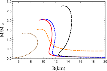
Figure 1: Mass-radius diagram obtained with five different EoSs. The solid red line corresponds to the SLy4 Douchin and Haensel (2001), the dashed blue line to the BL Bombaci and Logoteta (2018) and the black dashed dotted line to the MS1 Mueller and Serot (1996) EoSs. The brown dotted line corresponds to the piecewise polytropic defined in Eq. (12), see also the discussion below; the orange dashed dotted line corresponds to the hybrid star model defined in Eq. (16).

Next, we consider two EoSs built to study the effect of thermodynamic discontinuities. The piecewise polytropic EoS is defined as

$$p=\begin{cases}K_{1}\rho^{\Gamma_{1}}&\text{for }\rho<\rho_{t}\\ K_{2}\rho^{\Gamma_{2}}&\text{for }\rho>\rho_{t}\\ \end{cases}\,,$$ (12)

and we assume a transition density $\rho_{t}\simeq 2.98\rho_{\text{sat}}$, where the saturation density and pressure are respectively $\rho_{\text{sat}}\simeq 2.7\times 10^{14}\text{ g cm}^{-3}$ and $p_{\text{sat}}\simeq 4\times 10^{33}\text{ dyne cm}^{-2}$. In principle, $K_{1}$ and $K_{2}$ as well as $\Gamma_{1}$ and $\Gamma_{2}$ are the parameters describing the properties of matter in two different phases, see for example Shapiro and Teukolsky (1983). Here we employ a simplified approach aimed to reproduce the nuclear saturation point and based on the assumption that the matter density is continuous. In this way we obtain that

$$K_{1}=\frac{p_{\text{sat}}}{\rho_{\text{sat}}^{\Gamma_{1}}}\,,\qquad K_{2}=\frac{p_{\text{sat}}}{\rho_{\text{sat}}^{\Gamma_{2}}}\,,$$ (13)

At the interface, the speed of sound and the compressibility discontinuities can be expressed as

$$\Delta c_{s}^{2} =(c_{s2}^{2}-c_{s1}^{2})|_{t}=(\Gamma_{2}-\Gamma_{1})\frac{p_{t}}{\rho_{t}}\,,$$ (14)

$$\Delta\beta_{s} =(\beta_{s2}^{2}-\beta_{s1}^{2})|_{t}=\frac{\Gamma_{1}-\Gamma_{2}}{\Gamma_{1}\Gamma_{2}}\frac{1}{p_{t}}\,,$$ (15)

where $c_{s1}$ and $c_{s2}$ are the speeds of sound in the two phases. In this case one can even probe configurations with a nonmonotonic compressibility. In particular, we considered the model characterized by $\Gamma_{1}=2$, $\Gamma_{2}=3$, as well as $\Gamma_{1}=3$, $\Gamma_{2}=2$ that has a speed of sound jump $\Delta c_{s}=+0.05$ at the transition point . The TOV solutions for the latter case correspond to the dotted brown line in Fig. 1. In this case the maximum mass is $M\simeq 1.24M_{\odot}$ and the corresponding radius $R\simeq 6.6$ Km, for a central density $\rho_{c}\simeq 25.4\rho_{\text{sat}}$. The small values of mass and radius and the large value of the critical density are due to the fact we have considered a model in which part of the inner part is softer than the outer part.

Finally, we consider the hybrid star model with quark matter in the interior and an envelope described by a polytrope:

$$p=\begin{cases}K\rho^{\Gamma}&\text{for }p<p_{t}\\ c_{sq}^{2}(\rho-4B)&\text{for }p>p_{t}\\ \end{cases}$$ (16)

where $K=p_{\text{sat}}/\rho_{\text{sat}}^{\Gamma}$ (we tried to different values of $K$, with qualitatively the same results), $c_{sq}$ is the speed of sound of quark matter and we take the bag constant $B=(165\text{MeV})^{4}$. For the envelope we take $\Gamma=4/3$, as appropriate for a nonrelativistic electron gas. Unless differently stated, we use $c_{sq}^{2}=1/3$. At the transition point

$$K\rho_{1}^{\Gamma}=c_{sq}^{2}(\rho_{2}-4B)\,,$$ (17)

and the energy density discontinuity can be expressed as

$$\Delta\rho_{t}=\rho_{2}-\rho_{1}=\frac{K\rho_{1}^{\Gamma}}{c_{sq}^{2}}+4B-\rho_{1}\,,$$ (18)

and therefore

$$\frac{\partial\Delta\rho_{t}}{\partial\rho_{1}}=\frac{c_{se}^{2}-c_{sq}^{2}}{c_{sq}^{2}}=\frac{\Delta c_{s}^{2}}{c_{sq}^{2}}\,,$$ (19)

where $c_{se}^{2}=\Gamma p/\rho$ is the speed of sound squared in the envelope. In this case both $\Delta\rho_{t}$ and $\Delta c_{s}$ are nonzero. The corresponding TOV solution is reported in Fig. 1 by a orange dashed dotted line for $\rho_{2}=\rho_{1}$.

In principle one may consider more refined hybrid star models, see for example Alford et al. (2005); Chen et al. (2015), or piecewise polytropes, see Shapiro and Teukolsky (1983), however for our purposes it is enough to consider these relatively simple stellar models. Indeed, these models have the basic ingredients to test the properties of radial fluctuations in the presence of tunable speed of sound and/or energy density discontinuities. We notice that both models have a maximum mass that is below the observed $2M_{\odot}$ bound Demorest et al. (2010); Antoniadis et al. (2013); Rezzolla et al. (2018), however this is irrelevant for our purposes, because these models simply serve to test the numerical Numerov’s method and to study the effect of tunable discontinuities.

III Standing radial oscillations

Once the TOV stationary configuration has been determined, one can probe its stability towards collapse or explosion by considering a small harmonic radial perturbation of the form

$$\delta r=X(r)e^{i\omega t}\,,$$ (20)

where $X(r)$ and $\omega$ are respectively the amplitude and the frequency of the standing wave. The TOV stationary configuration is unstable if some stellar mode has an imaginary frequency. The conditions for the existence of standing waves are discussed in Cox (1983); here we shall restrict to adiabatic oscillations that conserve the total baryonic number that are slow with respect to the microscopic dynamics, see the discussion in Haensel et al. (1989). Within these restrictions, the linearized perturbation equations can be written as a second order homogenous differential equation

$$\omega^{2}e^{2(\lambda-\phi)}X=-c_{s}^{2}X^{\prime\prime}-\left((c_{s}^{2})^{\prime}-Z+4\pi r\gamma pe^{2\lambda}-\phi^{\prime}\right)X^{\prime}$$

$$-\left(2(\phi^{\prime})^{2}+\frac{2m}{r^{3}}e^{2\lambda}-Z^{\prime}+4\pi(p+w)Zre^{2\lambda}\right)X\,,$$ (21)

where

$$Z=c_{s}^{2}\left(\phi^{\prime}-\frac{2}{r}\right)\,,$$ (22)

while $\gamma$ and $c_{s}$ have been defined in Eq. (6), and therefore have the same value determined for the background. Following Bardeen et al. (1966), we redefine the radial displacement as

$$\xi=Xr^{2}e^{-\phi}\,,$$ (23)

in this way the differential Eq. (III) can be rewritten as a Sturm-Liouville differential equation

$$(H\xi^{\prime})^{\prime}=-(\omega^{2}W+Q)\xi\,,$$ (24)

where

$$H =r^{-2}(\rho+p)e^{\lambda+3\phi}c_{s}^{2}$$

$$Q =r^{-2}(\rho+p)e^{\lambda+3\phi}(\phi^{\prime 2}+4r^{-1}\phi^{\prime}-8\pi e^{2\lambda}p)$$

$$W =r^{-2}(\rho+p)e^{3\lambda+\phi}\,,$$ (25)

are the relevant background functions. This is a particularly convenient expression because the Lagrangian fluctuation of the pressure takes the simple expression

$$\Delta P =-c_{s}^{2}(p+\rho)r^{-2}e^{\phi}\,\xi^{\prime}\,,$$ (26)

and because the solution of Eq. (24) are known to be discrete: we will indicate with $\hat{\xi}_{n}$ the eigenmodes with $n$ nodes and with $\omega_{n}$ the corresponding frequency. The actual determination of the solution requires the study of the full numerical problem, including the appropriate boundary conditions.

III.1 Boundary conditions and interfaces

The differential Eq. (24) with the boundary conditions

$$\alpha_{1}\xi(0)+\alpha_{2}\xi^{\prime}(0) =0\qquad\alpha_{1}^{2}+\alpha_{2}^{2}>0\,,$$ (27)

$$\beta_{1}\xi(R)+\beta_{2}\xi^{\prime}(R) =0\qquad\beta_{1}^{2}+\beta_{2}^{2}>0\,,$$ (28)

forms a Sturmian system and it can be proved, see for instance Ince (1956), that $\omega_{n}^{2}$ are real and ordered

$$\omega_{n}^{2}<\omega_{n+1}^{2}\,,$$ (29)

meaning that the fundamental $0$th mode has the lowest frequency. For radial oscillations the boundary condition at the stellar center is

$$\xi(0)=0\,,$$ (30)

because the stellar center cannot be displaced, therefore it is equivalent to the condition in Eq. (27) with $\alpha_{2}=0$. However, the boundary condition at the stellar surface is not in general as in Eq. (28). The reason is that expanding the Sturm-Liouville equation close to the stellar surface one obtains, see for example Bardeen et al. (1966),

$$\xi^{\prime}_{n}=\gamma^{-1}R^{-1}(4+e^{2\lambda}M/R+\omega_{n}^{2}e^{-2\phi}(R^{3}/M))\xi_{n}\,,$$ (31)

which is similar to Eq. (28), but with the important difference that the Sturmian boundary condition does not depend on $\omega_{n}$. The only case in which Eq. (31) turns in Eq. (28) with $\beta_{2}=0$ is when $\gamma$ diverges at the stellar surface, as for strange stars. In this case $r=R$ is a regular point and all the solutions of Eq. (24) are regular at the stellar surface. If $\gamma$ is finite then $r=R$ is a regular singular point and there is an unphysical diverging solution.

These considerations led us to quest what are the general boundary conditions to be used for the regular solution of Eq. (24). Certainly, since it is an homogeneous differential equation the absolute value of the eigenfunction is irrelevant. As usual, we will use this freedom to set $\xi(R)=1$, in arbitrary units. To eliminate the diverging solution we show that it is enough to specify the boundary condition close to the stellar center where Eq. (24) admits two possible solutions

$$\xi=C_{1}(r^{3}+{\cal O}(r^{5}))+C_{2}(1+br^{2}+{\cal O}(r^{4}))\,,$$ (32)

where $C_{1}$ and $C_{2}$ are integration constants and $b$ depends on the background. Since the fluid at the stellar center cannot be displaced by a radial oscillation it follows that one has to take $C_{2}=0$ to eliminate the unphysical solution. In our numerical solution we will require that

$$\hat{\xi}_{n}\propto r^{3}\,,$$ (33)

and technically this will be done imposing the boundary conditions

$$\xi(r_{\text{min}})=C_{1}r_{\text{min}}^{3}\quad\text{and}\quad\xi^{\prime}(r_{\text{min}})=3C_{1}r_{\text{min}}^{2}\,,$$ (34)

where $r_{\text{min}}$ is the smallest radial distance considered in the integration of the TOV’s equation. Therefore, we take both boundary conditions close to the origin and we do not need an extra boundary condition at the surface. Let us insist on this aspect: the only boundary conditions that we impose to solve the differential equation are close to the stellar center. It is sometimes stated that one should impose a boundary condition at the stellar surface to avoid the unphysical diverging solution and thus enforce $\Delta P(R)=0$. Instead in our approach, the vanishing of the pressure fluctuations at the stellar surface is a consequence of the boundary conditions at the origin. In other words, any physical solution of the Sturm-Liouville differential equation with the correct boundary condition at $r=r_{\text{min}}$ does automatically satisfy the requirement that $\Delta P(R)=0$.

Regarding the radial dependence of $\Delta P$ it is maybe interesting to add few remarks. Since close to the stellar center the displacement field behaves as in Eq. (32), the pressure oscillation at the stellar center is well defined and given by

$$\Delta P_{c}=-3a_{\xi}c_{s,{c}}^{2}(p_{c}+\rho_{c})e^{\phi_{c}}\,,$$ (35)

where, as in Eq. (9), we have indicated with the subscript $c$ the values of the functions at the stellar center. Clearly $\Delta P_{c}$ is extremely small, because $\phi_{c}$ is large and negative. By increasing $r$ we know that the various quantities change as in Eq. (9), in particular $\phi(r)$ increases and the pressure oscillation exponentially grows. We also know that the pressure fluctuation vanishes at the stellar surface this means that $\Delta P(r)$ has at least a maximum, or a minimum. In Sec. IV we shall see that our numerical procedure is in agreement with this outlined behavior and the extremum of $\Delta P(r)$ is located very close to the stellar center.

We now turn to the interface between different stellar layers. The continuity of $\Delta P$ ensures that the system is always close to equilibrium. Since $\Delta P$ is a function of $\rho$ and $c_{s}^{2}$ it seems that any discontinuity of these quantities could produce a pressure jump. But this is unphysical, unless the perturbation arises in a time scale much shorter than the typical equilibrium timescale, which is not the case for the slow oscillations considered in the present article. Since $\phi$ is always a continuous function, from Eq. (26) we have that the continuity of the pressure perturbation implies that if $c_{s}^{2}(\rho+p)$ is discontinuous at a radial coordinate $\bar{r}$, then $\xi^{\prime}$ is discontinuous in $\bar{r}$. More precisely, we can say that if there is a shell of negligible depth, $\delta$, centered at $\bar{r}$ where $c_{s}^{2}(\rho+p)$ abruptly changes, then labeling with the $I$ ($E$) the quantities evaluated at the internal side (respectively external) side of the boundary, the continuity of the displacement and of the pressure imply that

$$\xi_{I}=\xi(\bar{r}-\delta) \simeq\xi(\bar{r}+\delta)=\xi_{E}\,,$$

$$c_{s}^{2}(\rho+p)\xi^{\prime}|_{I} \simeq c_{s}^{2}(\rho+p)\xi^{\prime}|_{E}\,,$$ (36)

meaning that $\xi$ is a continuous function and although $\xi^{\prime}$ is discontinuous in $\bar{r}$, the combination $c_{s}^{2}(p+\rho)\xi^{\prime}$ is always a continuous function.

IV The numerical method

We have developed an extended Numerov discretization method for the solution of the Sturm-Liouville equation (24) that takes into account the appropriate boundary conditions in Eq. (34), as well as the possible speed of sound and density discontinuities in Eq. (36). The method consists in discretizing the radial coordinate in $N$ steps transforming the Sturm-Liouville differential equation in an eigenvalue problem Glass and Harpaz (1983). The advantage of our procedure with respect to other methods, see for example Bardeen et al. (1966); Kokkotas and Ruoff (2001), is that it simultaneously provides many radial frequencies and eigenmodes, and no unphysical solution appears if one properly imposes the boundary conditions in Eq. (34). Moreover, there is a number of check that can be used to test the convergence of the method.

The proposed extended Numerov method works as follows. The Sturm-Liouville differential equation, see Eq. (24), can be written as

$$A_{1}\xi^{{}^{\prime\prime}}+A_{2}\xi^{{}^{\prime}}+A_{3}\xi=\omega^{2}\xi\,,$$ (37)

where $A_{1},A_{2}$ and $A_{3}$ can be obtained by expanding Eq. (24) using the coefficients in Eq. (25). Then we discretize the radial coordinate as

$$r_{n}=n\epsilon\,,$$ (38)

where $\epsilon=R/N$ and $n=1,\dots,N$. We define $\xi({r_{i}})=\xi_{i}$ and $A_{1n}=A_{1}(r_{n})$, $A_{2n}=A_{2}(r_{n})$ and $A_{3n}=A_{3}(r_{n})$ in such a way that Eq. (37) turns in

$$A_{1n}\xi^{{}^{\prime\prime}}_{n}+A_{2n}\xi^{{}^{\prime}}_{n}+A_{3n}\xi_{n}=\omega^{2}\xi_{n}\,,$$ (39)

and then we can cast Eq. (39) as the eigenvalue problem

$$A\bm{\xi}=\omega^{2}\bm{\xi}\,,$$ (40)

where $\bm{\xi}^{t}=(\xi_{1},...,\xi_{N})$ and $A$ is the matrix obtained by expressing the radial derivatives as finite differences. We can discretize the radial derivatives at any desired order; we checked that the method works considering the lowest order expansion of the derivatives but we used

$$\xi^{\prime}_{n} =\frac{\xi_{n-2}-8\xi_{n-1}+8\xi_{n+1}-\xi_{n+2}}{12\epsilon}+{\cal O}(\epsilon^{4})$$

$$\xi^{\prime\prime}_{n} =\frac{-\xi_{n-2}+16\xi_{n-1}-30\xi_{n}+16\xi_{n+1}-\xi_{n+2}}{12\epsilon^{2}}+{\cal O}(\epsilon^{3})\,,$$ (41)

where $\xi^{\prime}_{n}\equiv\xi^{\prime}(r_{n})$ and $\xi^{\prime\prime}_{n}\equiv\xi^{\prime\prime}(r_{n})$. The discretized version of Eq. (37) for $2<n<N-2$ is

$$\omega^{2}\xi_{n} ={\xi_{n-2}}\left(\frac{{A_{2n}}}{12\epsilon}-\frac{{A_{1n}}}{12\epsilon^{2}}\right)+{\xi_{n-1}}\left(\frac{4{A_{1n}}}{3\epsilon^{2}}-\frac{2{A_{2n}}}{3\epsilon}\right)$$

$$+\xi_{n}\left({A_{3n}}-\frac{5{A_{1n}}}{2\epsilon^{2}}\right)+\xi_{n+1}\left(\frac{4{A_{1n}}}{3\epsilon^{2}}+\frac{2{A_{2n}}}{3\epsilon}\right)$$

$$+{\xi_{n+2}}\left(-\frac{{A_{1n}}}{12\epsilon^{2}}-\frac{{A_{2n}}}{12\epsilon}\right)=\sum_{m=n-2}^{n+2}a_{nm}\xi_{m}\,,$$ (42)

which defines the matrix entries $a_{nm}$ for $2<n<N-2$ and $2<m<N-2$. All the other matrix elements are, for the time being, zero, indeed one cannot use the above definitions for the first two and last two rows of $A$.

IV.1 Boundaries

We first discuss how to implement the boundary condition close to the stellar center, properly defining the first two rows of the matrix $A$ to impose Eq. (34). We recall that the implementation of these condition is extremely important to avoid the unphysical solution, which is proportional to $C_{2}$ in Eq. (32), and to quantize the eigenfrequencies. In agreement with Eq. (34), close to the stellar center the first two discretized values of any eigenmode should be

$$\xi_{1}=C_{1}r_{\text{min}}^{3}\qquad\text{and}\qquad\xi_{2}=C_{1}(r_{\text{min}}+\epsilon)^{3}\,,$$ (43)

where $r_{\text{min}}$ is the minimum value considered in the numerical integration of the TOV’s equation. Then, we require that

$$\omega^{2}\xi_{1} =a_{12}\xi_{2}\,,$$

$$\omega^{2}\xi_{2} =a_{21}\xi_{1}\,,$$ (44)

which is the simpler way to link the first two values of the displacement close to the stellar center. Obviously, we do not know $\omega$, therefore it seems that we cannot fix the values of $a_{12}$ and $a_{21}$. However, from the above equations we obtain that $a_{12}a_{21}=\omega^{4}$, and

$$\frac{a_{12}}{a_{21}}=\left(\frac{r_{\text{min}}}{r_{\text{min}}+\epsilon}\right)^{6}\,,$$ (45)

which determines the ratio between these two matrix elements. Suppose that we fix the eigenmode, for simplicity $\omega^{4}=1$, then we have that

$$a_{12}=\frac{1}{a_{21}}=\left(\frac{r_{\text{min}}}{r_{\text{min}}+\epsilon}\right)^{3}\,,$$ (46)

and thus these matrix elements are now fixed. Now, if we define the top left corner of $A$ using Eq. (44), therefore as the block matrix

$$\left(\begin{array}[]{cc}0&a_{12}\\ a_{21}&0\end{array}\right)\,,$$ (47)

we are actually imposing that any eigenfunctions has the boundary conditions of Eq. (43). This will result in two spurious eigenvalues $\omega^{2}=\pm 1$ in the spectrum. In the end, since we know the values of these two spurious eigenvalues, we can easily identify and remove them as well as the corresponding eigenvectors.

Regarding the stellar surface, we do not impose any boundary condition. To define the matrix elements at the stellar surface, or more precisely the rows $N-1$ and $N$ of the $A$ matrix, we cannot use the discretization of the first and second derivatives of Eq. (41). The reason is that the background quantities are not defined for $r>R$ and therefore the $\xi_{N+1}$ and $\xi_{N+2}$ elements are unphysical. We tried different extrapolation method, which however lead us to different results. Thus we redefine the derivatives close to the $r=R$ boundary as

$$\xi^{\prime}_{N-1} =\frac{-\xi_{N-4}+6\xi_{N-3}-18\xi_{N-2}+3\xi_{N-1}+10\xi_{N}}{12\epsilon}$$

$$\xi^{\prime}_{N} =\frac{\xi_{N-4}-16/3\xi_{N-3}+12\xi_{N-2}-16\xi_{N-1}+25/3\xi_{N}}{4\epsilon}$$

$$\xi^{\prime\prime}_{N-1} =\frac{-\xi_{N-4}+4\xi_{N-3}+6\xi_{N-2}+11\xi_{N-1}-20\xi_{N}}{12\epsilon}$$

$$\xi^{\prime\prime}_{N} =\frac{11\xi_{N-4}-56\xi_{N-3}+114\xi_{N-2}-104\xi_{N-1}+35\xi_{N}}{12\epsilon}$$ (48)

meaning that for $n=N-1$ and $n=N$ we have that

$$\omega^{2}\xi_{n}=\sum_{m=N-4}^{N}a_{nm}\xi_{m}\,,$$ (49)

where the $a_{nm}$ coefficients for $N-1\leq n\leq N$ and $N-4\leq m\leq N$ can be determined inserting the Eqs. (48) in Eq. (39).

IV.2 Interfaces

We now consider how to discretize the differential equation close to $\bar{r}$, corresponding to the interface where the speed of sound and/or the matter density are discontinuous. The continuity of the pressure oscillation in Eq. (26) implies that $\xi^{\prime}(\bar{r})$ is discontinuous and that $\xi^{\prime\prime}(\bar{r})$ is a Dirac delta function. One therefore needs to isolate the discontinuity and properly expand on the left and on the right of $\bar{r}$. We remark that in any case it is important to obtain an expression that is “symmetric” around the discontinuity. In principle one is tempted to define the left-derivative for $r<\bar{r}$ and the right derivative for $r>\bar{r}$, but this method does not work with the Numerov discretization. The reason is that in this way one would obtain a block diagonal matrix, with a separation between interior modes and exterior modes. One could connect the left and right derivatives by inserting an additional intermediate point, however we found a better and faster way to deal with the discontinuity.

First, we isolate the discontinuous point: For any $N$ we build the set $r_{1},\dots,r_{N}$ according to Eq. (38) and we select $k$ such that $\bar{r}-r_{k}>0$ is a minimum and we define $\delta<\epsilon$ asking that $r_{k}+\delta>\bar{r}$ and $r_{k+1}-\delta<\bar{r}$. Then, we use the fact that $c_{s}^{2}(p+\rho)\xi^{\prime}$ is a continuous function of $r$, see Eq. (36). It follows that for any $r$ in the neighborhood of $\bar{r}$ defined as $|r-\bar{r}|<\delta$

$$\xi^{\prime}S|_{r-\delta}\simeq\xi^{\prime}S|_{r}\simeq\xi^{\prime}S|_{r+\delta}\,,$$ (50)

where the scaling function is defined as

$$S(r)\equiv c_{s}^{2}(p+\rho)\,,$$ (51)

and the value of the sound speed and of the energy density in $r$ depends on whether $r$ is smaller or bigger than $\bar{r}$. By expanding the displacement function on the left and on the right of $\bar{r}$, multiplying by the scaling function and taking into account Eq. (50), we can express the first and the second derivative in the symmetric forms

$$\xi^{\prime}_{k} =\frac{S(r_{k}+\delta)(\xi_{k+1}-\xi_{k})+S(r_{k}-\delta)(\xi_{k}-\xi_{k-1})}{2\epsilon S(r)}$$

$$\xi^{\prime\prime}_{k} =\frac{S(r_{k}+\delta)(\xi_{k+1}-\xi_{k})-S(r_{k}-\delta)(\xi_{k}-\xi_{k-1})}{\epsilon^{2}S(r)}\,,$$ (52)

where $\xi_{k}=\xi(r_{k})$, $\xi^{\prime}_{k}=\xi^{\prime}(r_{k})$ and $\xi^{\prime\prime}_{k}=\xi^{\prime\prime}(r_{k})$ and we have used the leading order expansion of the symmetric derivative. As a check, if $S(r)$ is continuous in $r$, the above expressions give the standard discretized definition of the first and second derivatives. Upon substituting Eq. (52) in Eq. (37) one obtains the matrix elements $a_{lm}$ with $l=k,k+1$ and $m=l-1,l,l+1$. Therefore, around the discontinuous interface the matrix equation (40) can be written as

$$\omega^{2}\xi_{l}=\sum_{m=l-1}^{l+1}a_{lm}\xi_{m}\,,$$ (53)

and thus, taking into account all the above discussion, the form of the $A$ matrix in Eq. (40) turns to

$$A=\left(\begin{array}[]{cccccccccccccc}0&a_{12}&0&0&0&0&0&\cdots&0&0&0&0&0&0\\ a_{21}&0&0&0&0&0&0&\cdots&0&0&0&0&0&0\\ a_{31}&a_{32}&a_{33}&a_{34}&a_{35}&0&0&\cdots&0&0&0&0&0&0\\ 0&a_{42}&a_{43}&a_{44}&a_{45}&a_{46}&0&\cdots&0&0&0&0&0&0\\ \vdots&&&&&&\ddots&&&&&&&\vdots\\ \vdots&&&&&&a_{kk-1}&a_{kk}&a_{kk+1}&&&&&\vdots\\ \vdots&&&&&&&a_{k+1k}&a_{k+1k+1}&a_{k+1k+2}&&&&\vdots\\ \vdots&&&&&&&&&\ddots&&&&\vdots\\ 0&0&0&0&0&0&0&\cdots&a_{N-3N-5}&a_{N-3N-4}&a_{N-3N-3}&a_{N-3N-2}&a_{N-3N-1}&0\\ 0&0&0&0&0&0&0&\cdots&0&a_{N-2N-4}&a_{N-2N-3}&a_{N-2N-2}&a_{N-2N-1}&a_{N-2N}\\ 0&0&0&0&0&0&0&\cdots&0&a_{N-1N-4}&a_{N-1N-3}&a_{N-1N-2}&a_{N-1N-1}&a_{N-1N}\\ 0&0&0&0&0&0&0&\cdots&0&a_{NN-4}&a_{NN-3}&a_{NN-2}&a_{NN-1}&a_{NN}\end{array}\right)$$

where the first two lines and the last two lines have the peculiar form determined in Sec. IV.1 to describe the stellar center and surface, respectively. The two central lines have to be inserted to take into account the interface discontinuities. In principle, one can consider an EoS with an arbitrary number of discontinuities: the corresponding $A$ matrix would then be a generalization of the one shown above, with an additional matrix element for each interface discontinuity.

V Numerical results and checks

Here we report the results obtained with the extended Numerov method using the method presented in the previous section and the EoSs discussed in Sec. II. We will first analyze the microscopic EoSs, characterizing the radial displacement and pressure and doing a number of numerical checks. Then we turn to the EoSs with tunable parameters.

V.1 Microscopic equations of state

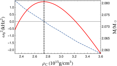
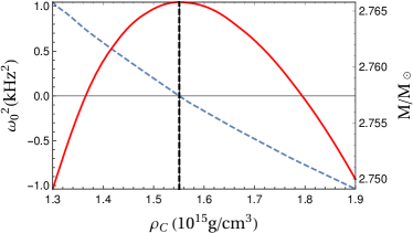
Figure 2: Masses and fundamental eigenfrequencies as a function of the stellar central density for three different EoSs, from top to bottom: SLy4, BL, MS1, see Sec. II for more details. The solid red lines correspond to the mass, in units of the solar mass, the dashed blue lines correspond to the frequency squared of the fundamental mode. The null mode appears when the dashed blue line intersects the horizontal axis, which is exactly the same central density where the gravitational mass reaches the maximum value. The vertical dashed line indicates the null mode while the solid vertical line indicates the maximum stellar mass. These two lines perfectly overlap.

In Fig. 2 we show the mass and the fundamental eigenfrequency as a function of the central density for the three microscopic EoSs discussed in Sec. II. For these three cases the last stable configuration, corresponding to the null mode, coincides with the maximum mass.

Regarding the radial eigenfunctions, we find that those obtained with the microscopic EoSs are similar, thus we only show the results obtained with the SLy4 EoS. In Fig. 3 we report the first three radial eigenmodes obtained with the SLy4 EoS for $\rho_{c}=0.98\times 10^{15}$ g/cm³, corresponding to a star with mass $M\simeq 1.4M_{\odot}$ and radius $R\simeq 11.4$ km, obtained with $N=1500$ discretized points. The obtained curves are smooth and we checked that the interpolated functions and the corresponding eigenfrequencies are solutions of the differential equation governing the radial fluctuations with an error of the order of few percent. An important nontrivial check is that the numerically obtained radial displacements have the correct behavior at the boundaries, that is close to the stellar center and the stellar surface. Sufficiently close to the stellar center the radial displacement of any mode should behave as

$$\hat{X}_{n}(r)=r^{-2}\hat{\xi}_{n}(r)e^{\phi}\propto r\,,$$ (54)

which follows from Eq. (23) and (33). Since in the numerical procedure we impose Eq. (43), this is a test that we correctly implemented this condition in the discretization method. In other words that adding the block matrix in Eq. (47) to the top-left corner of the matrix $A$ does provide the correct behavior close to the stellar center. On the other hand, from Eq. (31) we have that

$$X^{\prime}_{n}=a+\omega_{n}^{2}R^{3}/Me^{-2\phi}X_{n}\qquad\text{at}\quad r=R\,,$$ (55)

where $a$ is a constant that depends on the background configuration whose explicit expression can be obtained from Eq. (31). The relevant aspect is that $a$ does not depend on $n$. Note that in the numerical procedure we have not imposed this condition, indeed we have discretized close to the right boundary using the discretized left derivatives in Eq. (48).

From the plot reported in Fig. 3 one can qualitatively see that the correct linear behavior is reproduced close to the stellar center, as in Eq. (54), and that close to the stellar surface the derivative of the radial displacement increases with increasing $n$, as in Eq. (55), indeed we recall that $\omega_{n}<\omega_{n+1}$ and we fixed $\xi_{n}(R)=1$ for any mode. More precisely, we find that the linear behavior close to the stellar center as well as the relation in Eq. (31) close to the stellar center are satisfied with great accuracy, for instance with the piecewise polytropic we have an error less than $\sim 0.1\%$ already with $N=500$ discretized steps. Note that close to the stellar surface the radial displacement steeply increase: this is due to the fact that this is region corresponds to the crust, that is light as compared to the stellar interior.

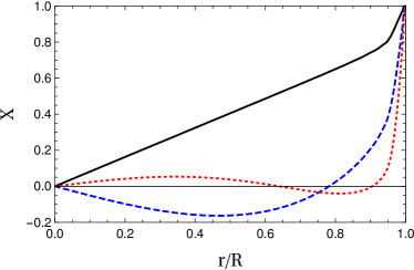
Figure 3: First three radial eigenmodes as a function of the radial coordinate obtained using the SLy4 EoS at $\rho_{c}=0.98\times 10^{15}$ g/cm³ by the extended Numerov method with $N=500$ discretized points. The displacement has been normalized to $1$, in arbitrary units, at the stellar surface. In agreement with Eq. (54), close to the stellar center the displacements are linearly dependent on the radial coordinate. In agreement with Eq. (55), close to the stellar surface the derivative of the displacement increases with $n$.

In Fig. 4 we show how the displacement of the $0$th radial mode (top panel) and the corresponding pressure oscillations (bottom panel) changes for the stellar configurations obtained by the SLy4 EoS at different central densities. In particular, we show the results obtained with three different values of the central density corresponding to stellar configurations with mass $M\simeq 1M_{\odot}$ (solid line), $M\simeq 1.4M_{\odot}$ (dashed line) and to the maximum mass $M\simeq 2.05M_{\odot}$ (dotted line). The extended Numerov method correctly reproduces the linear behavior close to the boundaries. For small central densities, the displacement is peaked at the stellar surface, but with increasing central density it tends to become smoother because more massive stars have a smaller crust.

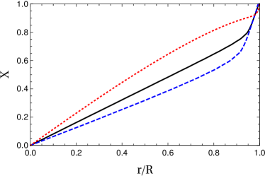
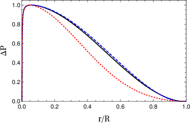
Figure 4: Displacement of the fundamental mode (top) and corresponding Lagrangian fluctuations of the pressure (bottom) obtained with the SLy4 EoS. The dashed line corresponds to the case $\rho_{c}=0.73\times 10^{15}$ g/cm³, mass $M\simeq 1M_{\odot}$ and radius $R\simeq 11.3$ km, the solid line corresponds to $\rho_{c}=0.98\times 10^{15}$ g/cm³, mass $M\simeq 1.4M_{\odot}$ and radius $R\simeq 11.4$ km and the dotted red line to the last stable configuration with $\rho_{c}=2.846\times 10^{15}$ g/cm³, mass $M\simeq 2.05M_{\odot}$ and radius $R\simeq 9.9$ km. The numerical algorithm correctly reproduces the linear behavior close to the stellar center. The pressure oscillations is normalized to the value at the peak.

The profile of the Lagrangian oscillations of the pressure shown in the bottom panel of Fig. 4 are obtained by Eq. (26). They reach an extremely small value at the stellar center, in agreement with Eq. (35), then they exponentially increase with $r$, due to the $e^{\phi}$ term in Eq. (26), reaching a maximum at a short radial distance from the stellar center. The position of the peak is almost insensitive to the stellar configuration considered: the maximum pressure is always located close to the stellar center. The only difference is that with increasing central density the peak becomes slightly narrower. In all the considered case the pressure oscillation vanishes at the stellar surface. Unfortunately, it does not seem to be possible to infer from this plot that the red dotted line corresponds to the last stable configuration.

V.2 Piecewise polytropic and hybrid equations of state

In Fig. 5 we report the mass and the fundamental eigenfrequency as a function of the central density for the the piecewise polytropic and the hybrid EoSs discussed in Sec. II. The first has a speed of sound discontinuity, while the second has a speed of sound as well as a matter density discontinuity. Although it is a small effect, we find that in both cases the last stable configurations, corresponding to the null mode, have a central density exceeding the one corresponding to the maximum mass, meaning that there may exist twin stellar configurations with the same gravitational mass but different radii. The results shown for the piecewise polytropic have been obtained with $\Gamma_{1}=3$ and $\Gamma_{2}=2$, but swapping the two values we do not find any appreciable increase of the central energy differences.

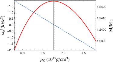
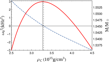
Figure 5: Mass and fundamental frequency as a function of the stellar central density for the piecewise polytope of Eq. (12), top panel, and the hybrid EoS in Eq. (16), bottom panel. The solid line corresponds to the mass, in units of the solar mass, the dashed line corresponds to the frequency squared of the fundamental mode. In both cases the null mode appears at a central density exceeding the value for which the gravitational mass reaches the maximum value, therefore the last stable configuration is not the one with the maximum mass. The vertical dashed line indicates to the null mode while the solid vertical line indicates the maximum stellar mass.

The profiles of the radial displacement and of the Lagrangian pressure oscillation obtained with the piecewise polytrope of Eq. (12) are shown in Fig. 6. In this case the derivative of the radial displacement is discontinuous at the interface where the speed of sound is discontinuous, which is in agreement with Eq. (36). Notice that the interior solution tends to grow more steeply then the external one, which is due to the fact that the derivatives of the displacement at the interface are related by Eq. (36) and the speed of sound on the left of the interface is smaller than the speed of sound on the right of the interface. Basically, at the interface the interior radial displacement bends to cope with the rapid crust displacement. We checked that the kink of $\xi^{\prime}$ at the interface agrees with Eq. (50) with great accuracy (the error is at the level of the used numerical accuracy). Notice that the pressure oscillation shown in the bottom panel of Fig. 6 is continuous and differentiable at any point. It is indeed very similar to the one obtained with the microscopic EoSs discussed above.

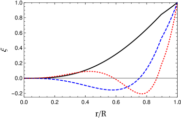
Figure 6: Radial profile of the displacement of the fundamental mode (top panel) and of the Lagrangian pressure fluctuation induced by the fundamental mode (bottom panel) for the piecewise polytropic EoS, see Eq. (12), for $\rho_{c}=6.5\times 10^{15}$ g cm^-3. The displacement has a small kink at the interface where the speed of sound is discontinuous. The pressure oscillations is normalized to the value at the peak, it is continuous and differentiable at any point.

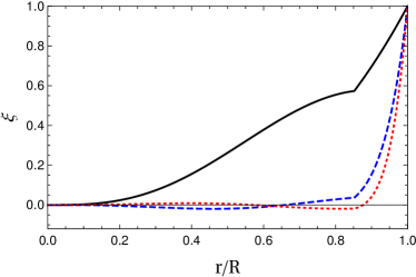
Figure 7: Radial profile of the displacement of the first three modes (top panel) and of Lagrangian pressure fluctuation induced by the fundamental mode (bottom panel) for the hybrid EoS, see Eq. (16), for $c_{s}^{2}=1/3$ and $\rho_{c}=3.25\times 10^{15}$ g cm^-3. The kink of $\xi$ corresponds to the interface where the matter density is discontinuous. The pressure oscillations is normalized to the value at the peak. The pressure is continuous but, although not visible in the plot, has a small kink at the interface.

Then we turn to the stellar model described by the hybrid EoS in Eq. (16). We show in Fig. 7 the displacement and the pressure oscillation. Both are continuous and have a kink at the interface between the core and the envelope, but the pressure kink is extremely small and not visible. Note that the displacement of the interior solution tends to become flat, as for self-bound objects, see the discussion after Eq. (31). As in the previous case at the interface the displacement bends to cope with the crust displacement.

In our simple model we can tune the interface energy density jump $\Delta\rho_{t}$ defined in Eq. (18) to emphasize the effect. By changing $\rho_{1}$, which is the largest possible density of the envelope, we can explore how large the energy density difference

$$\Delta\rho_{c}=\rho_{c0}-\rho_{cM}\,,$$ (56)

can be, where $\rho_{cM}$ is central energy density corresponding to the maximum gravitational mass and $\rho_{c0}$ is the central energy density corresponding to the appearance of the null mode. In Fig. 8 we report the plot of $\Delta\rho_{c}$ as a function of $\Delta\rho_{t}$ for the hybrid stellar model defined in Eq. (16) with $c_{sq}\simeq 0.28$ and $\Gamma=4/3$. The small value of the speed of sound has been chosen to further emphasize the effect of the interface energy density jump. The resulting maximum mass is about $0.5M_{\odot}$, which is indeed small, due to the fact that a small speed of sound implies a large compressibility. If one considers different values of $c_{sq}$ or $\Gamma$ one obtains similar results, but the effect is even less visible.

Figure 8: Difference between the central energy densities of the last stable configuration and of the maximum stellar mass, Eq. (56), as a function of the energy density discontinuity at the interface between strange quark matter and the external envelope, see Eq. (18).

We report in Fig. 9 the radial profile of the energy density and of the pressure for twin hybrid stars having the same gravitational mass $M\simeq 0.5M_{\odot}$ and radii $R\simeq 7.43$ Km (dashed line) and $R\simeq 7.67$ Km solid line.

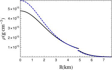
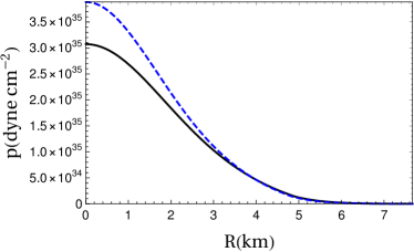
Figure 9: Radial profile of the energy density (top panel) and of the pressure (lower panel) for twin hybrid stars having the same gravitational mass $M\simeq 0.5M_{\odot}$ but different central densities: The dashed lines have been obtained considering central densities $\rho_{c}\simeq 5.9\times 10^{15}$ g cm^-3 while for the solid lines $\rho_{c}\simeq 4.8\times 10^{15}$ g cm^-3. The stellar radii are $R\simeq 7.43$ Km, dashed line, and $R\simeq 7.67$ Km, solid line.

From this figure it is clear that these twin stars have a similar envelope, but the more compact one accommodates more hadronic matter in the stellar interior. We emphasize that both twins are hybrid stars, but the more compact one has more strange matter than the other. We tried several different hybrid star configurations, finding that in any case the radius difference between the twin stars is of the order of hundreds of meters, therefore it is hardly observable.

VI Conclusions

We have developed an algorithm to quickly determine the eigenfrequencies and the eigenmodes of the stellar radial oscillations by discretizing the pertinent Sturm-Liouville differential equation. Our method is an extension of the Numerov’s method that takes into account the boundary conditions and the possible discontinuous interfaces. We find that the method is fast and precise for any considered EoS. Indeed, it gives radial displacements and pressure fluctuations that are smooth functions of the radial coordinate and that are in agreement with the foreseen behavior at the boundaries. Moreover, it allows us to reliably describe the interfaces between different states of matter.

An important aspect is that the extended Numerov method efficiently works for many different stellar model, as an example we considered three microscopic EoSs, a joined polytrope and an hybrid stellar models. In any considered case we find that the algorithm is very fast and the results are extremely stable for $N=1000$ discretized points. Taking $N=1500$ points we do not find any appreciable change in the eigenfrequencies or in the eigenmodes. Then, the diagonalization of the $N\times N$ matrix $A$ in Eq. (40) only requires few seconds on a laptop computer. The remarkable point is that in this way one obtains $N$ eigenfrequencies and eigenmodes, meaning that one can model with great accuracy any stellar radial oscillation by a Fourier decomposition.

In the presence of an interface discontinuity, the algorithm isolates the singular point and properly expands the displacement on the left and on the right of the discontinuity. We find that with a speed of sound or with a matter density discontinuity the last stable and the maximum mass configurations do not coincide. This allows the existence of twin compact stars, that is stars with the same mass but different radii. Therefore, we confirm the results of Vasquez Flores et al. (2012); Pereira et al. (2018) for hybrid stars and extend it to any piecewise polytropic solutions, even in the presence of only a speed of sound discontinuity. For hybrid stars we have tuned the density discontinuity to study how large can be the difference between the two critical densities finding that this difference tends to grow as depicted in Fig. 8. In any considered case, the radius difference between twin partners is small, of few hundred meters, at most, therefore they can be hardly discriminated by observation, if they exist.

In the present work we focused on the linear response analysis, however the nonlinear effects may qualitatively change the picture Dziembowski (1982); Gabler et al. (2009), with a much richer dynamics. It would be interesting to analyze the behavior of nonlinear effects in the presence of interface discontinuities.

Appendix A Damping

In the following we focus on the discontinuity in $c_{s}$ keeping $\rho$ continuous, but the procedure can be extended to the case with both discontinuous $c_{s}$ and $\rho$. Since $W,Q$ and $\xi$ are continuous function, we have from Eq. (24) that

$$(H\xi^{\prime})^{\prime}_{L}\simeq(H\xi^{\prime})^{\prime}_{R}\,,$$ (57)

and we notice that $H\xi^{\prime}=-\Delta Pe^{\lambda+2\phi}$, therefore we can rewrite the above equation as

$$(\Delta P_{L})^{\prime}+\Delta P_{L}(\lambda^{\prime}+2\phi^{\prime})_{L}\simeq(\Delta P_{R})^{\prime}+\Delta P_{R}(\lambda^{\prime}+2\phi^{\prime})_{R}\,,$$ (58)

where both $\phi^{\prime}$ and $\lambda^{\prime}$ are continuous functions, see Eqs. (11). It follows that if $\Delta P$ is continuous then also $\Delta P^{\prime}$ is continuous (this will not be the case when $\rho$ is discontinuous). Therefore, even in the presence of a speed of sound discontinuity $\Delta P$ is a smooth function of $r$.

The differential equation at the boundary allows us to explore the possible effect of wave damping in a certain region of the star. If we define $\alpha=c_{s}^{2}\xi^{\prime}$, then the interface condition in Eq. (57) can be written as

$$\alpha^{\prime}_{L}+K_{L}\alpha_{L}=\alpha^{\prime}_{R}+K_{R}\alpha_{R}$$ (59)

where

$$K=(B+E)/D\,$$ (60)

and

$$B =\log(r^{-}2e^{\lambda+3\phi})^{\prime}$$ (61)

$$D =e^{2(\phi-\lambda)}$$ (62)

$$E =D\frac{p^{\prime}+w^{\prime}}{p+\rho}\,.$$ (63)

The continuity of the pressure implies that $\alpha$ is a continuous function, but $K$ is discontinuous and this means that the relation between the second order derivatives of the displacement at the interface is nontrivial. However, in the special cases in which one phase is characterized by a large bulk viscosity, the pressure perturbation vanishes at the interface and $\xi$ is stationary (it has a maximum or a minimum) and then $\alpha_{L}=\alpha_{R}=0$. From Eq. (59) it follows that $\alpha^{\prime}_{L}=\alpha^{\prime}_{R}$. This special boundary condition is therefore

$$\xi^{\prime}_{L} =\xi^{\prime}_{R}=0$$ (64)

$$c_{L}^{2}\xi^{\prime\prime}_{L} =c_{R}^{2}\xi^{\prime\prime}_{R}\,.$$ (65)

If we further assume that $\xi^{\prime\prime}_{L}=\xi^{\prime\prime}_{R}=0$, we obtain that

$$\xi(\bar{r})=0\,.$$ (66)

Since the fundamental mode cannot have a node, it follows that only in this particular case one can really separate the modes as core modes and surface modes Gondek and Zdunik (1999), depending on whether the internal or external displacement is nonvanishing.

References

- Tolman (1939) R. C. Tolman, Phys. Rev. 55, 364 (1939).
- Oppenheimer and Volkoff (1939) J. R. Oppenheimer and G. M. Volkoff, Phys. Rev. 55, 374 (1939).
- Shapiro and Teukolsky (1983) S. Shapiro and S. Teukolsky, Black holes, white dwarfs, and neutron stars: the physics of compact objects, A Wiley-interscience publication (Wiley, New York, USA, 1983).
- Cox (1983) J. P. Cox, Theory of stellar pulsations (Princeton University Press, Princeton, USA, 1983).
- Chandrasekhar (1964a) S. Chandrasekhar, Phys. Rev. Lett. 12, 114 (1964a).
- Chandrasekhar (1964b) S. Chandrasekhar, Astrophys. J. 140, 417 (1964b), [Erratum: Astrophys. J.140,1342(1964)].
- Harrison et al. (1965) B. K. Harrison, K. S. Thorne, M. Wakano, and J. A. Wheeler, Gravitation Theory and Gravitational Collapse (Univ of Chicago, Chicago, USA, 1965).
- Chanmugam (1977) G. Chanmugam, Astrophys. J. 217, 799 (1977).
- Glass and Harpaz (1983) E. N. Glass and A. Harpaz, Mon.Not.Roy.Astron.Soc. 202, 159 (1983).
- Vaeth and Chanmugam (1992) H. M. Vaeth and G. Chanmugam, Astron.Astrophys. 260, 250 (1992).
- Gondek et al. (1997) D. Gondek, P. Haensel, and J. L. Zdunik, Astron. Astrophys. 325, 217 (1997), arXiv:astro-ph/9705157 [astro-ph] .
- Kokkotas and Ruoff (2001) K. Kokkotas and J. Ruoff, Astron. Astrophys. 366, 565 (2001), arXiv:gr-qc/0011093 [gr-qc] .
- Posada and Chirenti (2019) C. Posada and C. Chirenti, Class. Quant. Grav. 36, 065004 (2019), arXiv:1811.09589 [gr-qc] .
- Dziembowski (1982) W. Dziembowski, Acta Astronomica 32, 147 (1982).
- Gabler et al. (2009) M. Gabler, U. Sperhake, and N. Andersson, Phys. Rev. D80, 064012 (2009), arXiv:0906.3088 [gr-qc] .
- Haensel, P. et al. (2002) Haensel, P., Levenfish, K. P., and Yakovlev, D. G., A&A 394, 213 (2002).
- Burgio et al. (2011) G. F. Burgio, V. Ferrari, L. Gualtieri, and H. J. Schulze, Phys. Rev. D84, 044017 (2011), arXiv:1106.2736 [astro-ph.SR] .
- Alford and Harris (2019) M. G. Alford and S. P. Harris, Phys. Rev. C100, 035803 (2019), arXiv:1907.03795 [nucl-th] .
- Migdal (1971) A. B. Migdal, Zh. Eksp. Teor. Fiz. 61, 2209 (1971).
- Migdal (1972) A. B. Migdal, Soviet Physics Uspekhi 14, 813 (1972).
- Mannarelli (2019) M. Mannarelli, Particles 2, 411 (2019), arXiv:1908.02042 [hep-ph] .
- (22) K. Rajagopal and F. Wilczek, arXiv:hep-ph/0011333 [hep-ph] .
- Alford et al. (2008) M. G. Alford, A. Schmitt, K. Rajagopal, and T. Schafer, Rev. Mod. Phys. 80, 1455 (2008), arXiv:0709.4635 [hep-ph] .
- Anglani et al. (2014) R. Anglani, R. Casalbuoni, M. Ciminale, N. Ippolito, R. Gatto, et al., Rev. Mod. Phys. 86, 509 (2014), arXiv:1302.4264 [hep-ph] .
- Glendenning (2000) N. K. Glendenning, Compact stars: Nuclear physics, particle physics, and general relativity (Springer Verlag, New York, USA, 2000).
- Alcock et al. (1986) C. Alcock, E. Farhi, and A. Olinto, Astrophys.J. 310, 261 (1986).
- Haensel et al. (1986) P. Haensel, J. Zdunik, and R. Schaeffer, Astron.Astrophys. 160, 121 (1986).
- Benvenuto and Horvath (1991) O. G. Benvenuto and J. E. Horvath, Mon.Not.Roy.Astron.Soc. 250, 679 (1991).
- Datta et al. (1992) B. Datta, P. K. Sahu, J. D. Anand, and A. Goyal, Phys. Lett. B283, 313 (1992), arXiv:astro-ph/9304024 [astro-ph] .
- Gondek and Zdunik (1999) D. Gondek and J. L. Zdunik, Astron. Astrophys. 344, 117 (1999), arXiv:astro-ph/9901167 [astro-ph] .
- Vasquez Flores and Lugones (2010) C. Vasquez Flores and G. Lugones, Astronomy and relativistic astrophysics. Proceedings, 4th International Workshop, IWARA 2009, Maresias, Sao Paulo, Brazil, October 4-8, 2009, Int. J. Mod. Phys. D19, 1499 (2010).
- Salinas et al. (2019) M. Salinas, T. Klähn, and P. Jaikumar, Particles 2, 447 (2019).
- Haensel et al. (1989) P. Haensel, J. L. Zdunik, and R. Schaeffer, Astron.Astrophys. 217, 137 (1989).
- Sahu et al. (2002) P. K. Sahu, G. F. Burgio, and M. Baldo, Astrophys. J. 566, L89 (2002), arXiv:astro-ph/0111414 [astro-ph] .
- Vasquez Flores et al. (2012) C. Vasquez Flores, C. H. Lenzi, and G. Lugones, Proceedings, 5th International Workshop on Astronomy and Relativistic Astrophysics (IWARA2011): Joao Pessoa, Brazil, August 6-11, 2011, Int. J. Mod. Phys. Conf. Ser. 18, 105 (2012).
- Brillante and Mishustin (2014) A. Brillante and I. N. Mishustin, EPL 105, 39001 (2014), arXiv:1401.7915 [astro-ph.SR] .
- Pereira et al. (2018) J. P. Pereira, C. V. Flores, and G. Lugones, Astrophys. J. 860, 12 (2018), arXiv:1706.09371 [gr-qc] .
- Ince (1956) E. L. Ince, Ordinary Differential Equations, Dover Books on Mathematics (Dover Publications, Inc., New York, USA, 1956).
- Byron and Fuller (1992) F. W. Byron and R. W. Fuller, Mathematics of Classical and Quantum Physics, Vol. I and II, Dover Books on Physics (Dover Publications, Inc., New York, USA, 1992).
- Bardeen et al. (1966) J. M. Bardeen, K. S. Thorne, and D. W. Meltzer, Astrophys. J. 145, 505 (1966).
- Douchin and Haensel (2001) F. Douchin and P. Haensel, Astron. Astrophys. 380, 151 (2001), arXiv:astro-ph/0111092 [astro-ph] .
- Bombaci and Logoteta (2018) I. Bombaci and D. Logoteta, Astron. Astrophys. 609, A128 (2018), arXiv:1805.11846 [astro-ph.HE] .
- Mueller and Serot (1996) H. Mueller and B. D. Serot, Nucl. Phys. A606, 508 (1996), arXiv:nucl-th/9603037 [nucl-th] .
- Demorest et al. (2010) P. Demorest, T. Pennucci, S. Ransom, M. Roberts, and J. Hessels, Nature 467, 1081 (2010), arXiv:1010.5788 [astro-ph.HE] .
- Antoniadis et al. (2013) J. Antoniadis et al., Science 340, 6131 (2013), arXiv:1304.6875 [astro-ph.HE] .
- Rezzolla et al. (2018) L. Rezzolla, E. R. Most, and L. R. Weih, Astrophys. J. 852, L25 (2018), [Astrophys. J. Lett.852,L25(2018)], arXiv:1711.00314 [astro-ph.HE] .
- Alford et al. (2005) M. G. Alford, M. Braby, M. W. Paris, and S. Reddy, Astrophys.J. 629, 969 (2005), arXiv:nucl-th/0411016 [nucl-th] .
- Chen et al. (2015) H. Chen, J. B. Wei, M. Baldo, G. F. Burgio, and H. J. Schulze, Phys. Rev. D91, 105002 (2015), arXiv:1503.02795 [nucl-th] .