Angular momentum-related probe of cold gas deficiencies

Abstract

Recent studies of neutral atomic hydrogen (H i) in nearby galaxies found that all field disk galaxies are H i saturated, in that they carry roughly as much H i as permitted before this gas becomes gravitationally unstable. By taking this H i saturation for granted, the atomic gas fraction $f_{\rm atm}$ of galactic disks can be predicted as a function of the stability parameter $q=j\sigma/(GM)$, where $M$ and $j$ are the baryonic mass and specific angular momentum of the disk and $\sigma$ is the H i velocity dispersion (Obreschkow et al., 2016). The log-ratio $\Delta f_{q}$ between this predictor and the observed atomic fraction can be seen as a physically motivated ‘H i deficiency’. While field disk galaxies have $\Delta f_{q}\approx 0$, objects subject to environmental removal of H i are expected to have $\Delta f_{q}>0$. Within this framework, we revisit the H i deficiencies of satellite galaxies in the Virgo cluster and in clusters of the EAGLE simulation. We find that observed and simulated cluster galaxies are H i deficient and that $\Delta f_{q}$ slightly increases when getting closer to the cluster centres. The $\Delta f_{q}$ values are similar to traditional H i deficiency estimators, but $\Delta f_{q}$ is more directly comparable between observations and simulations than morphology-based deficiency estimators. By tracking the simulated H i deficient cluster galaxies back in time, we confirm that $\Delta f_{q}\approx 0$ until the galaxies first enter a halo with $M_{\rm halo}>10^{13}\rm M_{\odot}$, at which moment they quickly lose H i by environmental effects. Finally, we use the simulation to investigate the links between $\Delta f_{q}$ and quenching of star formation.

1 Introduction

Neutral atomic gas (H i) is found in most galaxies. It is a pivotal way-station in the evolution of galaxies: cooling accretion flows deliver H i gas to galactic disks (e.g. van de Voort & Schaye, 2012; Faucher-Giguère et al., 2015), where, given the right conditions, the H i can collapse into clouds and combine into molecular gas (H₂) and further into stars. In turn, H i can also be the exhaust product of stellar winds and supernovae and get pushed out of galactic disks by energetic feedback (e.g. Faber & Gallagher, 1976; Faucher-Giguère et al., 2015; Ford et al., 2013; Lagos et al., 2014).

Because of the physical importance of H i, the amount of this gas in a galaxy is a key parameter in galaxy evolution studies. However, since field disk galaxies span many ($>5$) orders of magnitude in stellar (and halo) mass, the most physically meaningful quantity is the atomic mass fraction, rather than the absolute amount of H i. In this work, the neutral atomic gas fraction of a galaxy is defined as

$$f_{\rm atm}\equiv\frac{1.35M_{\rm{HI}}}{M},$$ (1)

where $M=M_{*}+1.35(M_{\rm{HI}}+M_{\rm{H_{2}}})$ is the baryonic mass, $M_{*}$ is the stellar mass, $M_{\rm{HI}}$ is the H i mass, $M_{\rm{H_{2}}}$ is the molecular hydrogen mass and the factor 1.35 accounts for the universal Helium fraction, which is hard to measure directly on a galaxy-by-galaxy basis.

Observations of H i in rest-frame 21cm emission revealed that $f_{\rm atm}$ varies considerably between different galaxies (Maddox et al., 2015; Catinella et al., 2018; Chung et al., 2009). These empirical variations hold interesting clues on qualitatively different physics. However, a priori, it is not obvious whether these differences are due to internal differences (i.e. differences in other galaxy properties) or to external differences related to the galactic environment. In fact, both can be important. As for internal differences, it is well established that $f_{\rm atm}$ exhibits a weak but systematic dependence on stellar mass (Catinella et al., 2010) and a pronounced dependence on the morphology (Haynes & Giovanelli, 1984), size (Boselli & Gavazzi, 2009) and spin parameter (Huang et al., 2012) of the galactic disk. Even without an understanding of the causalities between these observables, it is thus clear that $f_{\rm atm}$ relates strongly to internal physics. In turn, it is also well established that $f_{\rm atm}$ can be strongly reduced by environmental effects, especially in dense cluster environments. Already early observations (e.g. Davies & Lewis, 1973; Giovanelli & Haynes, 1985) have found that spiral galaxies near the core region of clusters are very deficient in H i, compared to field galaxies of similar morphology and size. Many mechanisms can drive such deficiencies (see review Boselli et al., 2014b); for example (1) stripping of H i by the ram pressure of the hot intra-cluster medium Gunn & Gott, 1972, (2) tidal stripping by gravitational forces (Merritt, 1983), (3) heating by dynamical friction causing the H i to be ‘harassed’ (Moore et al., 1996), (4) merger-driven starbursts consuming a lot of H i (Hopkins et al., 2006) and (5) suppressed supply of new gas despite ongoing star formation (strangulation) (Peng et al., 2015).

In studying environmental effects on H i, it is crucial to separate the most important internal effects on $f_{\rm atm}$ from external ones. In other words, we would like to measure the deficiency (or excess) in $f_{\rm atm}$ due to external effects. The definition of such a ‘deficiency’ parameter is not obvious, as it requires to calibrate the typical H i content of galaxies against a property that is not (or significantly less) affected by the environment than the cold gas reservoir. From an observational point of view, the concept of H i deficiency has originally been introduced by Haynes & Giovanelli (1984) as the difference, in terms of $\log(f_{\rm atm})$, between the observed H i mass and the value expected for a field galaxy with the same morphological type and optical diameter. While empirical, this relation is based on the assumption that environment affects H i without affecting the optical size. Admittedly, this definition has hampered a quantitative comparison with predictions from theoretical models for which visual morphologies cannot be easily obtained. Thus, in recent years, significant effort has gone into calibrating new H i-deficiency parameters using physical quantities directly comparable with predictions from models. Among them, the combination of stellar surface density and ultraviolet colour presented by Catinella et al. (2010, 2018) is the one that mimics most closely the original definition, and has allowed detailed comparisons with semi-analytical models of ram-pressure and starvation (see Cortese et al., 2011). Conversely, calibrations based on just stellar mass or optical luminosity perform quite poorly as mass is a poor predictor of $f_{\rm atm}$ (see Catinella et al., 2010; Brown et al., 2015).

An interesting alternative to an empirical calibration of $f_{\rm atm}$ is offered by a recently proposed parameter-free physical model for $f_{\rm atm}$ in disk galaxies (Obreschkow et al., 2016, hereafter O16). An empirical extension of this model to other baryonic components has recently been presented by Romeo (2020) (see also Romeo & Mogotsi, 2018). The O16 model (detailed in Section 2) relies on the assumption that disk galaxies (as defined in the next paragraph) contain as much H i as they can in a gravitationally stable manner, given their baryonic mass $M$ and baryonic specific angular momentum (sAM) $j=J/M$. Apart from the straightforward physical interpretation of this calibration, the model of O16 has the advantage that it can be applied to observational data in the same way as to numerical simulations (e.g. Stevens et al., 2018; Wang et al., 2018), hence allowing for an unbiased comparison.

In this paper, we use the O16 model to revisit H i deficiencies in the satellite galaxies of the Virgo cluster, studied in the VIVA survey (Chung et al., 2009), and compare these measurements to cluster galaxies in the EAGLE simulation (Schaye et al., 2015; Crain et al., 2015; McAlpine et al., 2016). The objective is to critically discuss the use of the O16 model as a diagnostics of environmental effects which affects primarily the gas fraction but not (or much less) $j$, as well as to use this model as a bridge between observations and simulations to better understand the nature and implications of such effects.

Throughout this work, we will concentrate on ‘disk’ galaxies, here defined as all objects showing a clear signature of global rotation in their H i velocity maps. These galaxies encompass spiral and irregular optical morphologies and they can exhibit environmental disturbances such as tidal or pressure-driven stripping. For comparison with cluster galaxies, we will use the term ‘field’ galaxies to denote objects, which are not part of a group/cluster, show no major companion and no signs of ongoing or past interactions/mergers in their H i maps.

This paper is organised as follows. We start by summarising the O16 model and defining a H i deficiency estimator based on this model (Section 2). Section 3 explores this H i deficiency in Virgo cluster galaxies and compares this deficiency to traditional estimators. Section 4 explores the OG16-based H i deficiency estimator in the EAGLE simulation and compares the results to observations. Conclusions and a summary are given in Section 5.

2 Physically motivated H i deficiency

In an effort to explain the observed correlations between the H i content and $j$ in field disk galaxies, O16 introduced an analytical model for the atomic gas mass that can be supported against gravitational collapse in a flat exponential disk with circular rotation. Relying on Toomre (1964) like stability considerations, they found that the maximum stable value of $f_{\rm atm}$ depends on the mass and kinematics of a disk through a single dimensionless parameter $q$, defined as

$$q=\frac{j\sigma}{GM},$$ (2)

where $G$ is the gravitational constant, $M$ and $j$ are the baryonic (stars+cold gas) mass and sAM and $\sigma$ is the one-dimensional velocity dispersion of the ‘warm’ H i gas. We take this dispersion to be $\sigma=10$ km/s, consistent with the observational results (Walter et al., 2008; Leroy et al., 2008) that nearby spiral galaxies exhibit a galaxy-independent and radius-independent dispersion between roughly 8 km/s and 12 km/s. Incidentally, this dispersion approximately corresponds to the thermal motion of hydrogen and the supersonic turbulence in the interstellar medium at a temperature of $10^{4}\rm\leavevmode\nobreak\ K$, characteristic for the phase transition from H ii to H i. To the extent that $\sigma$ is considered fixed by such fundamental physical considerations, the O16 model is completely parameter-free.

The exact relation between $q$ and $f_{\rm atm}$ depends on the rotation velocity as a function of radius. However, this effect of the rotation curve is small (see different lines in Figure 2 of O16) and the $q$–$f_{\rm atm}$ relation is generally well approximated by the truncated power law

$$f_{\rm atm}={\rm min}\{1,2.5q^{1.12}\}.$$ (3)

This function is plotted as the solid line in Figure 1.

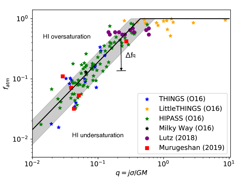
Figure 1: Atomic gas fraction versus the $q$-parameter for local field galaxies from different samples. The black line is the approximation (Eq. (3)) to the O16 model, with its uncertainty region due to the variance of the velocity dispersion shown as gray shading.

All field disk galaxies (as defined in Section 1) with sufficient H i and optical data for an accurate determination of $q$ and $f_{\rm atm}$, analysed so far, satisfy this relation within a log-normal scatter of about 0.16 dex standard deviation, as shown in Figure 1. The data shown here spans five orders of magnitude in stellar mass and include galaxies that have very high H i fractions (Lutz et al., 2018) and low H i fractions (Murugeshan et al., 2019) for their stellar mass and absolute $r$-band magnitude, respectively. In other words, these H i extreme galaxies have extremely high/low sAM $j$ for their mass (see Figure 12), but for their effective stability parameter $q$, their H i content is, in fact, normal. This result suggests that field disk galaxies in the local universe reside at the H i saturation point, approximated by Eq. (3). Interestingly, a recent analysis of cosmological zoom-simulations (Wang et al., 2018) showed that this statement holds true for most field disk galaxies at any redshift. This implies that Eq. (3) is a nearly universal and physically motivated relation for field disk galaxies.

Given the accuracy of the O16 model in predicting the H i mass of undisturbed galaxies, it seems sensible to define the H i deficiency of galaxies by their offset from Eq. (3), i.e. as

$$\Delta f_{q}={\rm log_{10}}\left({\rm min}\{1,2.5q^{1.12}\}\right)-{\rm log_{10}}\left(f_{\rm atm}\right).$$ (4)

The higher the value of $\Delta f_{q}$, the more H i deficient a galaxy is.

With respect to more common definitions of the H i deficiency (e.g. see Section 3.4), $\Delta f_{q}$ has the advantages that it can be directly interpreted as the H i deficiency relative to the saturation point and that it does not require any tuning to a reference sample. As we will demonstrate in the following, $\Delta f_{q}$ can be accurately measured in kinematic observations and simulations and thus offers a new bridge for comparing them in a like-to-like fashion.

3 Clues from the VIVA observation

3.1 Sample and data

To study the position of real cluster galaxies in the $(q,f_{\rm atm})$-plane, we rely on the data from the VLA Imaging of Virgo in Atomic gas (VIVA, Chung et al., 2009) survey. These data are optimal for this purpose because they provide us with spatially resolved 21cm spectral line data, showing both the amount of H i and its Doppler velocity along the line-of-sight at a spatial resolution of 15" (1.2 kpc at 17 Mpc). The use of such resolved kinematic data permits us to avoid the usual assumptions that (1) most material orbits the galaxy at the maximum circular velocity and (2) that this velocity is measured by the 21cm line width (e.g. $W_{50}$). In fact, both these assumptions, especially the second one, are hard to justify in stripped systems. The full VIVA sample counts 53 galaxies (48 spirals and 5 irregulars), all showing at least some rotation. In this sense and in terms of the range of stellar $j/M$ the VIVA sample is similar to the the THINGS sample.

Our analysis also requires stellar masses and optical sizes. These were drawn from the analysis of the GALEX-enhanced Herschel Reference Survey (HRS) data by Cortese et al. (2012), where stellar masses were derived using a ($g$-$i$)-colour-dependent mass-to-light ratio. Of the 53 VIVA objects, 41 are given stellar masses. We deliberately exclude merging or strongly interacting systems, where two galaxies are visibly connected in H i. These are four galaxies (NGC 4294/4299, NGC 4567/4568), of which one was already rejected because it had no separate stellar mass. This leaves us with a sample of 38 galaxies for the present analysis.

The definitions of $f_{\rm atm}$ and $q$ both refer to all baryons (stars+cold gas). Sometimes, the cold gas can have a significant molecular component. In the analysis of this paper, we include molecular masses determined from ¹²CO(1–0) emission in the cold gas study of the HRS (Boselli et al., 2014a). We used the data corresponding to a constant CO-to-H₂ conversion $X_{\rm CO}=2.3\cdot 10^{20}\rm\leavevmode\nobreak\ cm^{-2}/(K\leavevmode\nobreak\ km\,s^{-1})$ – the typical Milky Way value, not accounting for helium (Bolatto et al., 2013). Of our 38 galaxies, 37 have CO data. The molecular mass of the remaining object NGC 4606 is neglected.

All data are analysed assuming that the galaxies are situated at a distance of 17 Mpc, except for NGC 4380 and NGC 4424 which are assumed to lie at the Virgo B distance of 23 Mpc and NGC 4561 at a Hubble flow distance of 20.14 Mpc (following the HRS data).

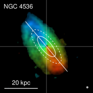
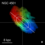
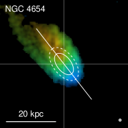
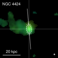
Figure 2: H i velocity-intensity maps of four galaxies in the VIVA sample. Stripping becomes stronger from the left to the right. Intensity represents the H i surface density (moment 0 map) as shown by the colorbar. The grey circles show the approximate resolution (FWHM) of $15^{\prime\prime}$. The orientation and aspect ratio of the ellipses show the position angle and inclination of the galaxies (from Chung et al., 2009). The sizes of these ellipses are such that they contain half of the $r$-band emission (solid) and H i (dashed).

3.2 Measurements

In order to measure $j$ of the stellar and cold gas components, we assume that the galaxies rotate in a thin disk and that the stars co-rotate around the galactic centre at the same velocity as the gas, hence neglecting so-called asymmetric drift due to the different dispersion of stars and gas. This approximation is consistent with spectroscopic observations in large late-type galaxies, but tends to over-estimate the stellar rotation by up to 20% in more dispersion-rich systems (Cortese et al., 2016). This error is comparable to other measurement uncertainties in $j$, e.g. due to inclination uncertainties (see the end of this section).

The sAM of stars ($j_{*}$) and H i ($j_{\rm HI}$) can be evaluated from the 2D kinematic data, some examples of which are shown in Figure 2. Explicitly, the $j$ values are computed as

$$j_{\rm phase}=\frac{\sum_{k}m_{k}r_{k}v_{k}}{\sum_{k}m_{k}},$$ (5)

where the sum goes over the pixels $k$ in the images and each pixel has a mass $m_{k}$, a galacto-centric radius $r_{k}$ and a circular velocity $v_{k}$. These three quantities are evaluated as follows.

• The mass map $\{m_{k}\}$ of H i is taken as the 21cm moment 0 map. For stars, the mass map is approximated by an exponential disk model, $m\propto\exp(-r/r_{d})$, where the scale radius $r_{d}$ is computed as $r_{d}=R_{e}/1.678$ with $R_{e}$ being the $r$-band effective radius from Cortese et al. (2012). Exponentials offer a good approximation of $j_{*}$ and allow us to extrapolate the optical data into the noise-dominated parts of the images (e.g. OG14; Romanowsky & Fall, 2012). In galaxies with a significant stellar bulge (i.e. the Sa-Sb types in the sample, such as NGC4606), $R_{e}/1.678$ underestimates the scale $r_{d}$ of the exponential profile at large radii, leading to an underestimation of $j_{*}$. This is partially compensated by the overestimation of $j_{*}$ caused by neglecting asymmetric drift.

• The radii $\{r_{k}\}$ in the plane of the galaxy are obtained from the radii $s_{k}$ in the plane of the sky using the standard deprojection equation $r=F(x,y;\alpha,i)s$ with a function $F$ that depends on the $(x,y)$-position in the image, as well as on the position angle $\alpha$ and inclination $i$ of the galaxy. The explicit expression can be found in Eq. (B3) of OG14.

• The circular velocities $\{v_{k}\}$ in the plane of the galaxy are computed from the line-of-sight velocities $v_{z}$ (1st moment of H i line) using the deprojection equation $v=C(x,y;\alpha,i)v_{z}$, given in Eq. (B4) of OG14.

The H i images of VIVA are large enough and deep enough (typical H i column density of 3–$5\cdot 10^{19}\rm\leavevmode\nobreak\ cm^{-2}$) for the values of $j_{\rm HI}$ to be converged within a few percents (based on the detailed convergence study in OG14). However, in some galaxies the optical disk extends beyond the H i disk, meaning that no velocity data is available in their outer parts. In these cases, the moment 1 map of H i is extrapolated beyond the observations assuming a flat rotation curve with a velocity fixed at the 90% quantile of the observed pixels. The relative increase of $j_{*}$ due to this extrapolation varies between 0% and $\sim 100\%$ with a mean of $25\%$. We caution, that this method bears some risk that the rotation curve has not yet reached the flat part, which would lead to an underestimation of $j_{*}$ and thus of $q$ and $\Delta f_{q}$. However, this effect must be small since the maximum H i velocity of our galaxy sample is consistent with the local baryonic Tully-Fisher relation (McGaugh & Schombert, 2015).

When deprojecting the data, care must be applied to divergencies: $F$ diverges for edge-on galaxies ($i=90^{\circ}$), whereas $C$ diverges for face-on galaxies ($i=0^{\circ}$), as well as on the minor axis for galaxies of any inclination. Measurement errors of pixels close to a divergency can lead to large uncertainties in $j$. To avoid this problem, the sums in Eq. (5) are only taken over pixels where $F<3$ and $C<3$. In other words, the observed radii and velocities are never multiplied by more than a factor 3 in the deprojection procedure. In axially symmetric galaxies, this rejection of pixels has no systematic effect on $j$, since the numerator and denominator in Eq. (5) are reduced by the same factor. Since the minimum of $\left|C\right|$ is $\sin^{-1}i$ (along the major axis), the requirement that $\left|C\right|<3$ implies that only galaxies with $\sin^{-1}i<3$, i.e. $i>20^{\circ}$ can be used. All galaxies in our sample satisfy this condition, since the minimum inclination is $30^{\circ}$.

In summary, we have measurements of the stellar $j_{*}=J_{*}/M_{*}$ and atomic $j_{\rm HI}=J_{\rm HI}/M_{\rm HI}$. As we do not have sufficient data for good measurements of molecular sAM values, $j_{\rm H_{2}}$, we assume that these values are identical to $j_{*}$. This is justified by the approximate congruence between molecular and stellar material in nearby star-forming galaxies (Walter et al., 2008). For heavily stripped galaxies, where both the H i and H₂ disks have been significantly truncated, $j_{\rm H_{2}}$ might be closer to $j_{\rm HI}$. However, a test of these heavily stripped galaxies ($\Delta f_{q}>0.5$) shows that their sAM changes only by about a percent if approximating $j_{\rm H_{2}}\approx j_{\rm HI}$ instead of $j_{\rm H_{2}}\approx j_{*}$. For the one galaxy without CO data, the H₂ mass is neglected. The error made in doing so is at most a few percent, based on the other 37 galaxies with CO data.

The baryonic sAM $j$ can then be computed as the mass-weighted mean sAM of the components,

$$j=\frac{J}{M}=\frac{(M_{*}+1.35M_{\rm H2})j_{*}+1.35M_{\rm HI}j_{\rm HI}}{M_{*}+1.35(M_{\rm HI}+M_{\rm H2})}.$$ (6)

where the factor 1.35 ensures that Helium is accounted for in the atomic and molecular component.

Measurement uncertainties of $j$ are computed through linear propagation of inclination uncertainties of $10^{\circ}$ and assuming an additional extrapolation error of $10\%$, roughly the uncertainty in the maximum rotation velocity used for this extrapolation.

In environmentally perturbed and stripped systems, the assumption of a flat disk at constant inclination and position angle potentially introduces significant systematic errors in $j$, which are hard to estimate. However, the H i mass fraction in stripped regions, is generally very small and often exaggerated in non-linear luminosity scales, such as in Figure 2. In fact, even in one of the most heavily stripped galaxies NGC 4424, only 35% of the H i resides in the non-symmetric tail and of the stellar mass fraction in this tail is significantly smaller. Neglecting this material only changes the resulting value of $q\propto j/M$ by a few percent.

All sAM measurements with statistical uncertainties are listed in Table 3.3. The table also lists the resulting values of $q$, computed using a fixed H i velocity dispersion of $\sigma=10$ km/s for all galaxies. This assumption (justified in Section 2) was made since the velocity resolution (10 km/s) of VIVA is insufficient for a direct measurement. The table also shows the atomic gas fractions $f_{\rm atm}$ and H i deficiencies, calculated using Eqs. (1) and (4), respectively. Where available molecular masses are included.

3.3 Results of the Virgo sample

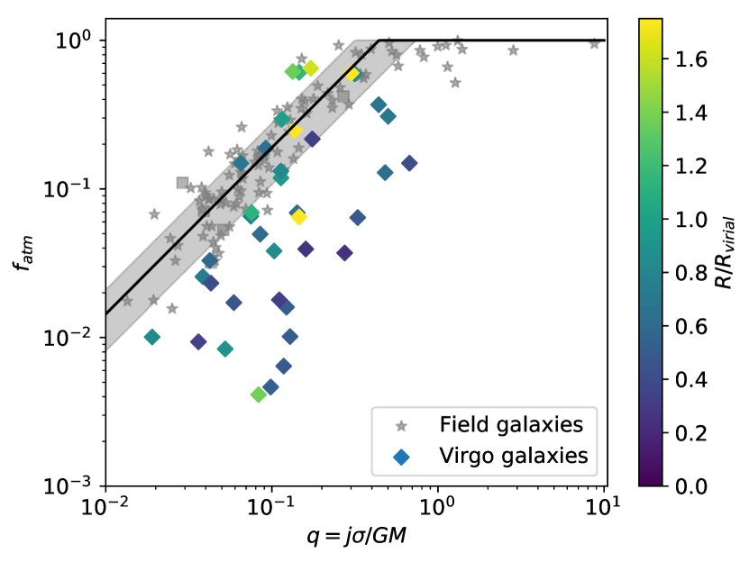
Figure 3: Atomic gas fraction versus parameter $q$. Diamonds are the Virgo galaxies from the VIVA survey. Gray points are the field galaxies from Figure 1. The color bar represents the ratio between projected distance to the giant elliptical galaxy M87 at the centre of Virgo A and the virial radius of Virgo A (1.55 Mpc, Ferrarese, et al., 2012).

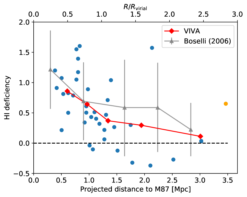
Figure 4: H i deficiency as a function of projected distance from galaxies to the cluster centre M87. The upper axis shows the distances normalized to the virial radius of 1.55 Mpc. The red diamonds show the mean value of $\Delta f_{q}$ in VIVA, binned by projected distance. The two right-most bins (distance $>1.6$ Mpc) are slightly wider to ensure that each bin contains at least three objects. The grey points and their uncertainty of 1$\sigma$ are from Figure 2 in Boselli & Gavazzi (2006), presenting the average H i deficiency in each bin from a larger, optically controlled sample. Their H i deficiencies are measured by Eq. 8 ($\Delta f_{D}$, detailed discussion in Sec 3.4.2). The orange point is NGC 4772, who is likely to have experienced a minor merger recently.

Table 1: Key properties of the galaxies in our subsample of VIVA. Columns are as follows. (1) Galaxy names; (2) stellar masses from Cortese et al. (2012), with a typical uncertainty $\sim$0.15 dex; (3) total H i mass from Chung et al. (2009); (4) H i mass uncertainty; (5) H₂ mass from Boselli et al. (2014a); (6) H₂ mass uncertainty; (7) half-mass radii in $r$-band from Cortese et al. (2012); (8) half-mass radii of H i (determined from the VIVA moment 0 maps); (9) stellar sAM; (10) sAM of H i; (11) typical uncertainty of $j_{*}$ and $j_{\rm HI}$; (12) parameter $q$; (13) neutral atomic gas fraction; (14) H i deficiency $\Delta f_{q}$. In the units, $\rm lg$ stands for the base-10 logarithm.

ID	$M_{*}$	$M_{\rm HI}$	$\Delta M_{\rm HI}$	$M_{\rm H_{2}}$	$\Delta M_{\rm H_{2}}$	$R_{\rm e}^{\rm opt}$	$R_{\rm e}^{\rm HI}$	$j_{*}$	$j_{\rm HI}$	$\Delta j$	$q$	$f_{\rm atm}$	$\Delta f_{q}$
–	$\!\!\!{\rm lg}(\rm M_{\odot})\!\!\!$	$\!\!\!{\rm lg}(\rm M_{\odot})\!\!\!$	$\!\!\!{\rm lg}(\rm M_{\odot})\!\!\!$	$\!\!\!{\rm lg}(\rm M_{\odot})\!\!\!$	$\!\!\!{\rm lg}(\rm M_{\odot})\!\!\!$	kpc	kpc	$\!\!\!{\rm lg}(\rm kpc\,km/s)\!\!\!$	$\!\!\!{\rm lg}(\rm kpc\,km/s)\!\!\!$	$\!\!\!{\rm lg}(\rm kpc\,km/s)\!\!\!$	–	–	–
(1)	(2)	(3)	(4)	(5)	(6)	(7)	(8)	(9)	(10)	(11)	(12)	(13)	(14)
IC 3392	9.77	7.69	0.34	8.62	0.19	2.60	1.60	2.56	2.20	0.05	0.129	0.010	1.39
NGC 4192	10.65	9.68	0.04	9.39	0.20	9.70	16.50	3.41	3.52	0.04	0.113	0.119	0.27
NGC 4216	11.00	9.30	0.09	9.21	0.20	6.30	13.60	3.22	3.66	0.04	0.038	0.026	0.40
NGC 4222	9.31	8.86	0.10	8.06	0.19	3.80	7.40	2.68	3.06	0.04	0.501	0.308	0.51
NGC 4254	10.39	9.70	0.04	10.02	0.05	5.10	9.90	3.06	3.30	0.21	0.065	0.149	-0.10
NGC 4298	10.10	8.75	0.08	9.16	0.18	3.90	4.10	2.75	2.71	0.07	0.085	0.050	0.50
NGC 4302	10.44	9.22	0.07	9.29	0.18	7.90	10.30	3.29	3.38	0.04	0.142	0.069	0.61
NGC 4321	10.71	9.51	0.02	9.91	0.05	8.10	10.70	3.33	3.34	0.18	0.075	0.066	0.32
NGC 4330	9.52	8.70	0.10	8.61	0.19	6.00	4.90	3.13	3.05	0.04	0.674	0.149	0.83
NGC 4351	9.17	8.53	0.06	8.11	–	2.60	2.90	2.21	2.17	0.09	0.175	0.217	0.21
NGC 4380	10.06	8.16	0.19	8.84	0.19	5.90	5.60	2.94	2.80	0.07	0.160	0.015	1.32
NGC 4383	9.42	9.52	0.05	8.48	0.09	1.40	9.90	1.94	3.16	0.06	0.277	0.595	-0.00
NGC 4388	10.14	8.62	0.26	8.78	0.20	5.00	4.50	3.26	3.04	0.04	0.275	0.037	1.20
NGC 4396	9.25	8.99	0.09	8.55	0.18	4.50	5.80	2.75	2.94	0.04	0.439	0.369	0.43
NGC 4402	10.04	8.62	0.18	9.31	0.05	4.70	4.10	3.00	2.77	0.04	0.160	0.039	0.91
NGC 4419	10.24	7.82	0.62	9.11	0.05	2.60	2.50	2.91	3.01	0.05	0.098	0.005	1.60
NGC 4424	9.91	8.34	0.07	8.86	0.18	5.20	6.70	2.35	2.01	0.06	0.054	0.031	0.48
NGC 4450	10.70	8.51	0.08	9.07	0.20	4.70	5.80	3.07	3.07	0.11	0.052	0.008	1.04
NGC 4457	10.43	8.34	0.11	9.19	–	2.00	2.50	2.38	2.38	0.18	0.019	0.010	0.47
NGC 4501	10.98	9.27	0.06	9.88	0.05	6.00	8.20	3.30	3.36	0.06	0.043	0.023	0.50
NGC 4522	9.38	8.58	0.13	8.90	0.18	4.10	4.10	2.93	2.81	0.04	0.481	0.129	0.89
NGC 4532	9.21	9.34	0.03	8.30	0.18	2.70	6.20	2.27	2.58	0.05	0.146	0.610	-0.32
NGC 4535	10.45	9.57	0.02	9.55	0.05	8.60	13.20	3.25	3.37	0.10	0.113	0.132	0.22
NGC 4536	10.26	9.73	0.02	9.45	0.05	7.80	12.80	3.20	3.33	0.05	0.137	0.248	0.04
NGC 4548	10.74	8.86	0.03	8.88	0.05	6.10	8.70	3.16	3.19	0.14	0.059	0.017	0.79
NGC 4561	8.99	9.20	0.03	8.57	–	2.40	5.40	1.83	2.54	0.18	0.149	0.591	-0.30
NGC 4569	10.66	8.85	0.10	9.69	0.05	8.70	4.90	3.41	3.00	0.05	0.111	0.018	1.07
NGC 4579	10.94	8.80	0.12	9.36	0.05	4.80	6.60	3.15	3.27	0.14	0.036	0.009	0.81
NGC 4580	9.99	7.50	0.34	8.60	0.18	2.50	1.20	2.57	2.32	0.13	0.083	0.004	1.57
NGC 4606	9.77	7.45	0.23	–	–	3.00	0.80	2.48	1.83	0.06	0.118	0.006	1.55
NGC 4607	9.60	8.39	0.16	8.80	0.19	3.50	3.30	2.87	2.76	0.04	0.329	0.064	1.05
NGC 4651	10.13	9.66	0.03	8.96	0.21	3.20	8.20	2.87	3.24	0.08	0.115	0.295	-0.12
NGC 4654	10.14	9.52	0.03	9.61	0.05	5.10	7.80	2.95	3.06	0.07	0.092	0.188	-0.04
NGC 4689	10.19	8.73	0.05	9.31	0.05	5.10	4.50	2.93	2.79	0.15	0.103	0.038	0.71
NGC 4698	10.52	9.27	0.03	8.65	–	4.30	16.90	3.00	3.55	0.05	0.076	0.069	0.30
NGC 4713	9.22	9.51	0.03	8.72	0.18	2.60	8.70	2.40	2.80	0.08	0.172	0.648	-0.27
NGC 4772	10.25	8.97	0.06	8.48	–	4.40	6.20	3.07	3.28	0.06	0.146	0.065	0.65
NGC 4808	9.49	9.61	0.03	8.59	0.19	2.40	12.40	2.42	3.25	0.05	0.300	0.603	0.03

The diamonds in Figure 3 show the 38 Virgo galaxies of our sample in the $(q,f_{\rm atm})$-plane. As expected, most of these galaxies lie below the analytical relation, in the H i undersaturated region. Almost all our Virgo galaxies, except for most of those right at the edge of the cluster (green–yellow colours in the figure), lie significantly ($>0.2$ dex) below the analytical relation, whereas almost of all field galaxies of the reference sample (grey stars) lie on the analytical relation. This suggests that the $(q,f_{\rm atm})$-plane is a useful diagnostic for the presence of environmental effects that do not significantly affect $q$. Indeed, in stellar mass-dominated galactic disks, $q$ only has a weak dependence on H i, which vanishes if $j_{*}=j_{\rm HI}$. Thus, even if H i is heavily stripped, $q$ only changes slightly. For instance, removing all the H i from the Milky Way would only decrease its $q$-value by $\sim 5\%$.

The offset of the galaxies from the analytical $q$–$f_{\rm atm}$ relation of H i saturated systems is quantified by $\Delta f_{q}$. Figure 4 shows this theoretically motivated ‘H i deficiency’ $\Delta f_{q}$ as a function of the projected distance of the galaxies to the central cluster galaxy M87. As naively expected and well-established (e.g. Davies & Lewis, 1973; Giovanelli & Haynes, 1985; Chung et al., 2009), there is a trend for the H i deficiency to increase with the proximity to the cluster centre. However, this qualitative statement is subject to a list of caveats:

• The decrease of $\Delta f_{q}$ with increasing radius is slightly stronger than observed in optically complete samples (gray points in Figure 4; Boselli & Gavazzi 2006), but the statistical significance of this tension is marginal because of the small number of objects.

• Some galaxies might already have had a peri-centre passage, where they might have been stripped of their H i content, even if now they are situated at large radii.

• Other environmental effects than stripping could have affected selected galaxies. For instance, NGC 4772 (the orange point in Figure 4) is likely to have experienced a minor merger recently (Haynes et al., 2000).

Numerical simulations, such as the one discussed in Section 4 can resolve these caveats, as they provide access to three-dimensional geometries and a look back in time.

3.4 Comparison between different H i deficiencies

Let us now compare the new H i deficiency estimator $\Delta f_{q}$ to two more familiar empirical estimators, mainly uses in simulation-based studies (Section 3.4.1) and observational environmental studies (Section 3.4.2), respectively.

3.4.1 H i deficiency relative to stellar mass

A simple way of defining a H i deficiency, often used for simulations (e.g. Crain et al., 2017; Stevens et al., 2019), is to measure the offset of a galaxy from the mean stellar mass-H i mass relation, or, equivalently the baryon mass-H i fraction relation, $M$–$f_{\rm atm}$. Formally, this definition of the H i deficiency can be written as

$$\Delta f_{M}={\rm log_{10}}\left[0.5\left(\frac{M}{10^{9}\rm M_{\odot}}\right)^{-0.37}\right]-{\rm log_{10}}\left(f_{\rm atm}\right),$$ (7)

where the first term on the right-hand-side denotes the mean value of $f_{\rm atm}$ at baryonic (stellar+cold gas) mass $M$ in a volume-complete sample of galaxies, given by O16 and consistent with the optically-selected GASS sample Catinella et al. (2010).

The advantage of this definition is its simplicity, only requiring global stellar mass (light) and H i-mass measurements. However, this simplicity comes at the cost of several disadvantages. Firstly, the definition of $\Delta f_{M}$ is purely phenomenological, providing no insight into the physical causes of H i-rich and H i-poor galaxies. Secondly, the $M$–$f_{\rm atm}$ distribution exhibits a large intrinsic scatter ($\sim 0.5$ dex, see O16 Figure 3), even for spiral galaxies that show no evidence of environmental effects, hence making $\Delta f_{M}$ a poor diagnostic of such effects. Thirdly, H i-selected samples are biased towards H i-rich galaxies in the $M$–$f_{\rm atm}$ space and therefore biased negatively in $\Delta f_{M}$. At least in field galaxies, this inherent bias towards H i-rich galaxies does not (or at most weakly) bias $\Delta f_{q}$, because the H i-rich systems are indeed the ones with high spin and thus high $q$, as shown in the Appendix Figure 12. However, we make the comparison here for reference.

Figure 5(a) shows the comparison of $\Delta f_{M}$ and $\Delta f_{q}$ in our sample of 38 Virgo galaxies. From this figure, $\Delta f_{M}$-$\Delta f_{q}$ is close to one-to-one relation despite a small offset ($\sim 0.1$ dex) due to aforementioned selection effects. In this case, $\Delta f_{M}$ can be used to identify H i deficient galaxies.

Cosmological simulations can bypass concerns of selection bias, since they are limited by mass and volume rather than sensitivity. Also, the mean $M$–$f_{\rm atm}$ relation (or $M_{*}$–$M_{\rm HI}$ relation) is well-defined. For instance, one can select all central galaxies (as opposed to satellites) to determine the median value of $M_{\rm HI}$ as a function of stellar mass and then compute the deficiency $\Delta f_{\rm M}$ of the satellites relative to this relation. Such an approach has been presented, for instance, by Crain et al. (2017) for the EAGLE simulations, Stevens et al. (2018) for the Illustris-TNG simulations and Lagos et al. (2011, 2018) for semi-analytic models.

3.4.2 H i deficiency relative to optical size

Traditional definitions of H i deficiencies, used in observational environmental studies, compare the H i mass of individual galaxies to that of field galaxies of the same optical size and (sometimes) same morphological type (Haynes & Giovanelli, 1984). Formally this can be written as

$$\Delta f_{\rm D}={\rm log_{10}}M_{\rm HI}^{\rm ref}-{\rm log_{10}}M_{\rm HI}^{\rm obs},$$ (8)

where $M_{\rm HI}^{\rm ref}$ is the expected H i mass of field galaxies and $M_{\rm HI}^{\rm obs}$ is the observed value of an individual object. The variation of $M_{\rm HI}^{\rm ref}$ with morphological type is often modelled as using a power law approximation

$${\rm log_{10}}h^{2}M_{\rm HI}^{\rm ref}={\rm A}+{\rm B}{\rm log_{10}}(h^{2}D^{2})$$ (9)

where $D$ is optical diameter (e.g. at the $25\rm\leavevmode\nobreak\ mag/arcsec^{2}$ isophote), $h\approx 0.7$ is the Hubble parameter and $A$ and $B$ are numerical constants. These constants are normally calibrated separately to each morphological Hubble type, such as shown in Table 3 of Boselli & Gavazzi (2009).

Indeed Figure 5(b) shows that $\Delta f_{D}$ and $\Delta f_{q}$ fall nearly on a one-to-one relation. This similarity between $\Delta f_{D}$ and $\Delta f_{q}$ can be understood from the fact that the galactic size is determined by the sAM (Fall & Efstathiou, 1980; Mo, Mao & White, 1998). However, in very high H i-rich galaxies, $\Delta f_{D}$ and $\Delta f_{q}$ will diverge. The value of $\Delta f_{D}$ can even be negative, while $\Delta f_{q}\sim 0$, because (1) the optical diameter is much smaller than the baryonic diameter, and (2) $\Delta f_{q}$ is based on the gas fraction, who has maximum value 1.

In environmental observational studies of H i, $\Delta f_{D}$ is widely used. However, in cosmological simulations, the definition and measurement of morphological types is somewhat cumbersome and thus $\Delta f_{D}$ is not normally used.

In summary, the estimator $\Delta f_{D}$ often has similar values to $\Delta f_{q}$, but the latter has the advantages of (1) being easily useable with observations and simulations, as well as (2) having a more straightforward physical interpretation in terms of the H i saturation point.

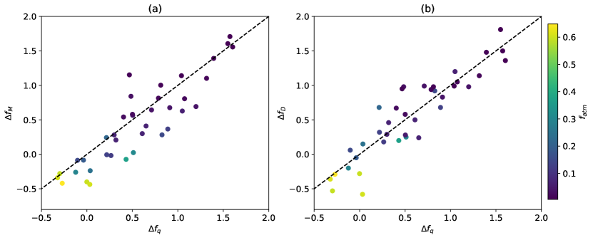
Figure 5: Comparison between the different H i deficiency estimators $\Delta f_{D}$, $\Delta f_{M}$ and $\Delta f_{q}$. The colour bar shows the atomic gas fraction. Dashed lines are the one-to-one relations.

4 Insights from the EAGLE simulations

In this section, we investigate how the cluster galaxies in a hydrodynamics cosmological simulation evolve in the $q-f_{\rm atm}$ plane. The advantage of such a simulation is that we can trace the history of the galaxies and explore the evolution of $f_{\rm atm}$ through cosmic time. We use the EAGLE simulation (Schaye et al., 2015; Crain et al., 2015; McAlpine et al., 2016), which successfully reproduce several statistical gas properties of a volume-complete sample, such as the total neutral gas (H i +H₂)-stellar mass relation (Bahé et al., 2016), the scaling relation between H₂ mass and stellar mass, star formation rate and stellar surface density of galaxies (Lagos et al., 2015), and reasonably well the H i-stellar mass relation of galaxies (Crain et al., 2017). Particularly relevant to our work are the results of Marasco et al. (2016), who showed that EAGLE reproduces the observed decrease in the H i-to-stellar mass ratio with increasing parent halo mass (up to $10^{14.75}\rm M_{\odot}$). We here use the largest EAGLE simulation box with a volume of $(100\,\rm Mpc)^{3}$, which contains 10 galaxy clusters of halo masses $>10^{14}\,\rm M_{\odot}$.

4.1 EAGLE simulation

The EAGLE simulation suite (details in Schaye et al. 2015, Crain et al. 2015 and McAlpine et al. 2016) consists of a large number of cosmological hydrodynamic simulations with different resolutions, cosmological volumes, run with a modified version of the parallel N-body smoothed particle hydrodynamics (SPH) code GADGET-3. The simulation follows the formation and evolution of galaxies and supermassive black holes in a standard $\Lambda$ cold dark matter universe, and uses several subgrid physics modules including (1) star formation (Schaye & Dalla Vecchia, 2008), (2) stellar evolution and chemical enrichment (Wiersma et al., 2009b), (3) radiative cooling and photoheating (Wiersma et al., 2009a), (4) stellar feedback (Dalla Vecchia & Schaye, 2012), and (5) black hole growth and active galactic nucleus (AGN) feedback (Rosas-Guevara et al., 2015). Table 2 provides the parameters of the Ref-L100N1504 simulation used in this paper.

Table 2: Basic properties of the EAGLE run Ref-L100N1504. Here, cMpc and ckpc refer to comoving Mpc and kpc, respectively, while pkpc refers to physical kpc.

	Property	Units	Value
(1)	Comoving box side $L$	cMpc	$100$
(2)	Number of particles		$2\times 1504^{3}$
(3)	Gas particle mass	$\rm M_{\odot}$	$1.81\times 10^{6}$
(4)	DM particle mass	$\rm M_{\odot}$	$9.7\times 10^{6}$
(5)	Gravitational softening length	ckpc	$2.66$
(6)	Max. gravitational softening length	pkpc	$0.7$

4.1.1 Calculation of the H i fraction

The temperature and density of the gas in EAGLE are calculated directly as part of the hydrodynamic simulation, accounting for radiative cooling and feedback processes using subgrid models. A global temperature floor, $T_{\rm eos}(\rho)$, is imposed, corresponding to a polytropic equation of state, $P\propto\rho^{\gamma_{\rm eos}}_{\rm g}$, where $\gamma_{\rm eos}=4/3$. This equation is normalised to give a temperature $T_{\rm eos}=8\times 10^{3}$ K at $n_{\rm H}=10^{-1}\,\rm cm^{-3}$, which is typical of the warm interstellar medium (e.g. Richings et al., 2014).

Hence, the ionised, atomic and molecular gas phases of the interstellar medium are not separated while running the simulation (and thus not fully consistent with the instantaneous star formation rates). Therefore, the amount of atomic material was calculated in post-processing by Lagos et al. (2015). They first computed the neutral (atomic+molecular) gas fraction of each particle following the prescription of Rahmati et al. (2013), which was calibrated to cosmological simulations coupled with full radiative transfer calculations. Rahmati et al. (2013) presented fitting functions to calculate the neutral fraction on a particle-by-particle basis from the gas temperature and density, and the total ionization rate (photoionization plus collisional ionization). Given the neutral gas fraction of a particle, Lagos et al. (2015) applied the Gnedin & Kravtsov (2011) model to split this gas further into its atomic and molecular phases. This model assumes that the dust-to-gas ratio and the radiation field are the driving processes setting the H i/H₂ ratio. It further assumes that the dust catalyses the formation of H₂, while the UV radiation destroys the dust, preventing the formation of H₂. Lagos et al. (2015) assume the dust-to-mass ratio to scale with the local gas metallicity and the radiation field to scale with the local surface density of the star formation rate.

Given this way of computing H i masses in EAGLE, we then compute the atomic gas fractions $f_{\rm atm}$ of each cluster galaxy using the definition of Eq. (1), as in the observations. The mass limit of the EAGLE simulation implies a H i mass limit close to $10^{7}\rm M_{\odot}$. Galaxies with less H i will be represented by zero H i mass. We account for this effect in our statistical analysis of Section 4.4.

4.1.2 Calculation of the $q$ parameter

The parameter $q$ remains as defined in Eq. (2). We assume $\sigma=10$ km/s for the H i and the global $j$ is calculated via:

$$j=\frac{M_{*}j_{*}+1.35M_{{\rm gas}}j_{{\rm gas}}}{M_{*}+1.35\,M_{{\rm gas}}},$$ (10)

where $M_{*}$ and $j_{*}$ are the mass and sAM of stars, and $M_{\rm gas}$ and $j_{\rm{gas}}$ are the mass and the sAM of the neutral hydrogen (H i ​+H₂). This equation slightly differs from Eq. (6), because the neutral gas phases have been combined into a mean $j_{\rm{gas}}$ in Lagos et al. (2017), but note that this does not affect the global baryonic $j$. Lagos et al. computed $j_{*}$ and $j_{\rm gas}$ by summing over all relevant particles $k$,

$$j_{\rm phase}=\left|\frac{\Sigma_{k}m_{k}\textbf{r}_{k}\times\textbf{v}_{k}}{\Sigma_{k}m_{k}}\right|,$$ (11)

where $m_{k}$ are the particle masses and $\textbf{r}_{k}$ and $\textbf{v}_{k}$ are the position and velocity vectors, relative to the centre-of-mass. To estimate $j_{*}$, they used star particles only, while the estimation of $j\rm{{}_{gas}}$ made use of all gas particles that have a neutral gas fraction $>0$. Lagos et al. showed that the stellar $M_{*}$–$j_{*}$ relation in EAGLE galaxies of different morphologies has good agreement with measurements in the local universe by Romanowsky & Fall (2012); Obreschkow & Glazebrook (2014); Cortese et al. (2016).

The resolution limit of the simulation constrains the galaxy selection. Schaye et al. (2015) suggested that the results are consistent between the simulations being used here and higher resolution, smaller volume simulations for $M_{*}\geq 10^{9}\,M_{\odot}$. Lagos et al. (2017) showed that the estimation of $j_{*}$ is converged for $M_{*}\geq 10^{9.5}\,\rm M_{\odot}$ (see their Appendix A). We analyze galaxies with $M_{*}\geq 10^{9.5}\,\rm M_{\odot}$ in this paper.

4.1.3 EAGLE clusters

In EAGLE, haloes are identified using a friend-of-friends algorithm (FoF, Davis et al., 1985). There are 10 clusters with $M_{\rm halo}\geqslant 10^{14}\,\rm M_{\odot}$ and 205 smaller clusters (or ‘massive groups’) with $10^{13}\,\rm M_{\odot}\leqslant M_{\rm halo}<10^{14}\,\rm M_{\odot}$ at $z=0$. In this paper, we use the 10 massive clusters for comparing $\Delta f_{q}$ between EAGLE and VIVA (Section 4.2), while we also include the smaller clusters in the following time-evolution analysis (Section 4.3) for increased statistical power.

We measure the distance of satellite galaxies from the centre of their cluster and compare the results with the observation. The coordinates of each galaxy are available from the EAGLE public database (McAlpine et al., 2016). We use the centre of potential of the FoF group as the cluster centre and measure the 3D distance to the satellites in units of $R_{200}$ (of the particular cluster). The shapes of the clusters are irregular because they are defined by as FoF groups. We select the galaxies at $z=0$ that lie within less than $1.75R_{200}$ from the cluster centres, regardless of whether these galaxies belong to the cluster, to do our analysis and comparison.

4.2 H i fraction in EAGLE cluster galaxies at $z=0$

We now compare the VIVA data against a comparable sample of EAGLE cluster galaxies. For consistency between the two data set, we only consider the 10 most massive EAGLE clusters ($M_{\rm halo}>10^{14}\,\rm M_{\odot}$), of which we select the satellite galaxies at radii $<1.75R_{200}$ and with $M_{*}>10^{9.5}{\rm M_{\odot}}$, $M_{\rm HI}>10^{7.45}\rm M_{\odot}$ and $q>0.01$. The $M_{*}$ cut is, in fact, necessary because of the resolution of the simulation (see Section 4.1.2), but it happens to be an almost perfect match to the VIVA sample, which has just four objects slightly below $10^{9.5}\rm M_{\odot}$ ($10^{9.22\pm 0.15}\rm M_{\odot}$ being the smallest value). The $M_{\rm HI}$ cut matches the minimum value in the VIVA subsample (see Table 3.3). Likewise, the selection $q>0.01$ is approximately consistent with the $q$-range in VIVA. Furthermore, this criterion effectively corresponds to a morphology selection to disk dominated galaxies (as constant values of $q\propto j/M$ approximately correspond to different morphologies Obreschkow & Glazebrook, 2014). Overall, this selection results in a sample of 200 galaxies across all 10 clusters. Note that EAGLE used a FoF algorithm to determine whether a galaxy belongs the cluster or not. Of the 200 galaxies, 117 physically belong to a cluster in this sense, while the remaining 83 are close to the cluster, but do not belong to the FoF.

Before using the selected sample of EAGLE cluster galaxies to study H i deficiencies $\Delta f_{q}$, we first check if similarly selected field galaxies are indeed H i saturated in the sense of Eq. (3). To this end, we consider the simulated galaxies with halo masses $10^{11}{\rm M_{\odot}}<M_{\rm halo}\leqslant 10^{12}{\rm M_{\odot}}$ and exclude those who have satellites and have been moving into a cluster/massive group in the past. Apart from this criterion, we apply exactly the same selection as for the EAGLE cluster galaxies, that is $M_{*}>10^{9.5}{\rm M_{\odot}}$, $M_{\rm HI}>10^{7.45}\rm M_{\odot}$ and $q>0.01$. This results in a sample of 2100 field galaxies. Field galaxies suffer less from environmental effects and are thus expected to be H i saturated.

Figure 6 shows the $\Delta f_{q}$-histograms of EAGLE field and cluster galaxies. The simulated field galaxies exhibit a peak near $\Delta f_{q}\sim 0.2$, while cluster galaxies are scattered to significantly larger values of $\Delta f_{q}$, demonstrating that the simulated cluster galaxies are indeed more frequently H i deficient than the field galaxies. The fact that the mean of field galaxies is $\Delta f_{q}\sim 0.2$ rather than $\Delta f_{q}\sim 0$ is likely caused by a slight underestimation of the H i mass in EAGLE (for galaxies in this halo mass range), also seen in an the offset of $M_{\rm HI}-M_{*}$ relative to observations (see Figure 7 in Crain et al., 2017). In principle, one could introduce an ad hoc correction of $0.2\rm dex$ for the simulated $\Delta f_{q}$-values at $z=0$. However, since this correction is small compared to the typical values of stripped galaxies and systematic uncertainties in the determination of $\Delta f_{q}$, we decided not to apply such a correction.

Figure 7 shows the EAGLE cluster galaxies in the $q-f_{\rm atm}$ plane (at $z=0$). Most of the simulated satellite galaxies lie in the H i undersaturated region, similarly to the observational data (Figure 3). An advantage of the simulation is that we can investigate the causes of H i deficiencies. Following Marasco et al. (2016), the dominant cause of H i deficiencies in EAGLE clusters more massive than $10^{14}\,\rm M_{\odot}$ is ram pressure stripping, with a significant secondary contribution from high-speed satellite-satellite encounters, causing dynamical heating of the cold gas. Tidal stripping plays a negligible role in our EAGLE satellites, but becomes important in group-scale haloes ($<10^{13}\,\rm M_{\odot}$).

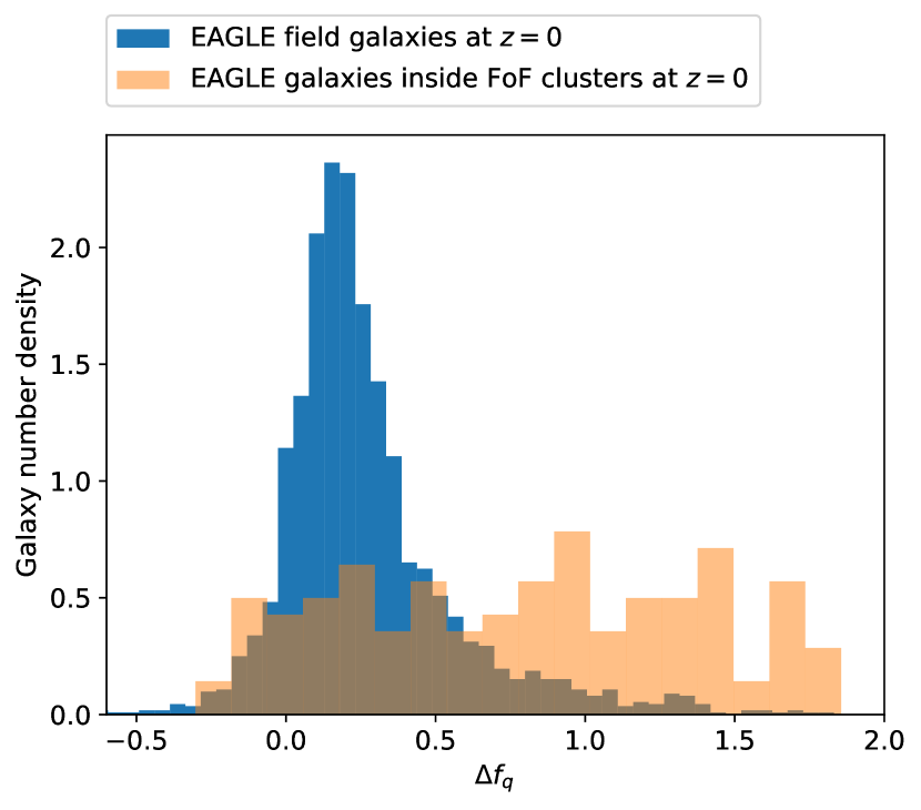
Figure 6: Number density of EAGLE field and cluster galaxies as a function of $\Delta f_{q}$. The median and standard deviation of the field galaxies are 0.20 and 0.29, respectively. The median and standard deviation of the cluster galaxies (in the FoF) are 0.85 and 0.58, respectively. The cluster galaxies show a much more significant positive tail into the stripped regime. The $p$-value of the Kolmogorov-Smirnov test for these two distributions is $10^{-5}$, comfirming that the two distributions are different.

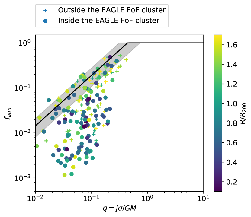
Figure 7: ($q,f_{\rm atm}$)-distribution of the EAGLE satellite galaxies in clusters with $M_{\rm halo}>10^{14}\rm M_{\odot}$, selected as described in Section 4.2. The circles are identified inside the (FoF) clusters while the crosses are outside the (FoF) clusters. The solid line and shading show the $q-f_{\rm atm}$ relation for field galaxies as in Figure 1. The colour bar shows the 3D distance from the satellite galaxies to the cluster centre.

In Figure 8, we show the $\Delta f_{q}$-distance relation in EAGLE compared to VIVA and samples from Boselli & Gavazzi (2006). We find that the tendency of galaxies to become more H i deficient as they get closer to the cluster centre is qualitatively similar in EAGLE and VIVA. Quantitatively the trend is more pronounced in VIVA because, as we mentioned in Section 3.3, VIVA lacks statistical power because of the limited number of galaxies at a radii $\gtrsim 2$ Mpc. In line with this explanation, the EAGLE data is more consistent with the H i deficiency trend of an complete optically selected sample (binned grey points in Figure 8).

The simulated data in Figure 8 shows very large scatter at all distances from the cluster centre. This scatter is probably attributed to similar effects as in empirical data (see bullet points in Section 3.3), that is the clusters are not fully relaxed, galaxies at identical radii have very different histories, some galaxies have mutual interactions that affect their H i, etc. Furthermore, galaxies at the same distance from the cluster centre may reside in different intra-cluster medium (ICM) densities, because large clusters are generally not spherically symmetric. In EAGLE this is clear from the fact that many galaxies outside the spherical radius $R_{200}$ lie still within the FoF group (blue dots at $R>R_{200}$), while other galaxies inside this spherical radius lie outside the FoF group (purple crosses at $R<R_{200}$). Likewise, real clusters are often aspherical (Jauzac, et al., 2016; Stroe, et al., 2015).

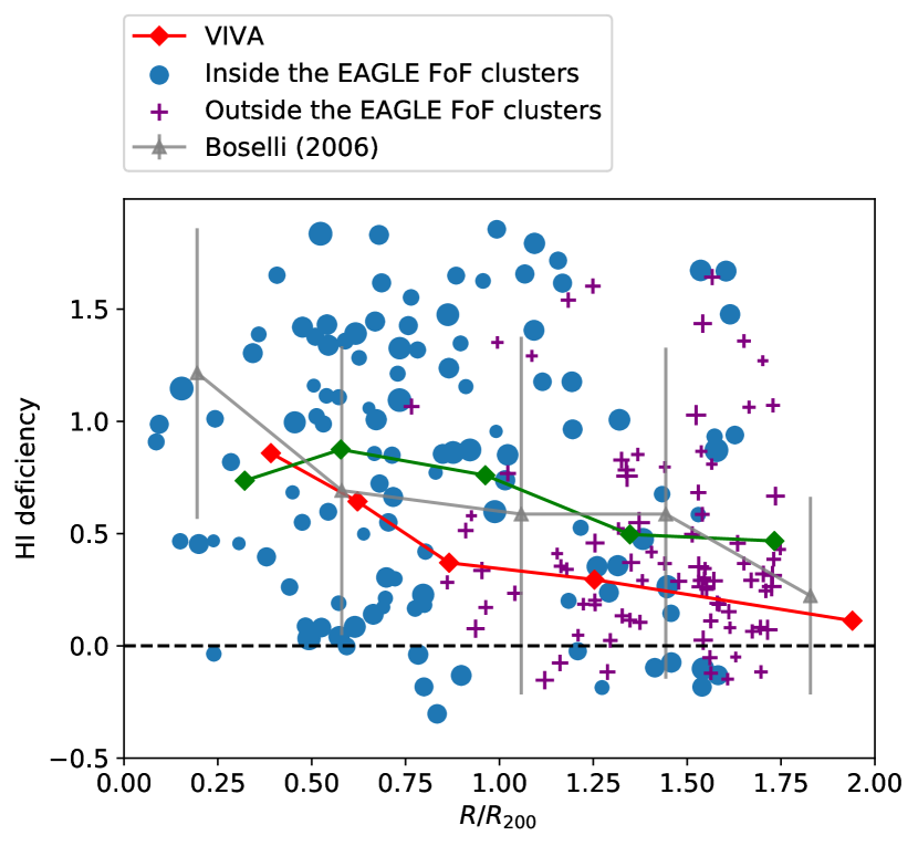
Figure 8: $\Delta f_{q}$ as a function of the 3D distance to the centre of potential of EAGLE galaxies. The blue points represent the galaxies inside the friends-of-friends (FoF) group of the clusters. In turn, the purple crosses denote galaxies outside the FoF groups. The bigger the size of the symbols, the larger the baryonic mass of a galaxy. The green diamonds and line represent the mean value of all the selected EAGLE galaxies in different radius bins. As in Figure 4, the red line is the $\Delta f_{q}$-distance relation from VIVA and the grey points are from the optical sample of Boselli & Gavazzi (2006). All data are normalized to the virial radius 1.55 Mpc.

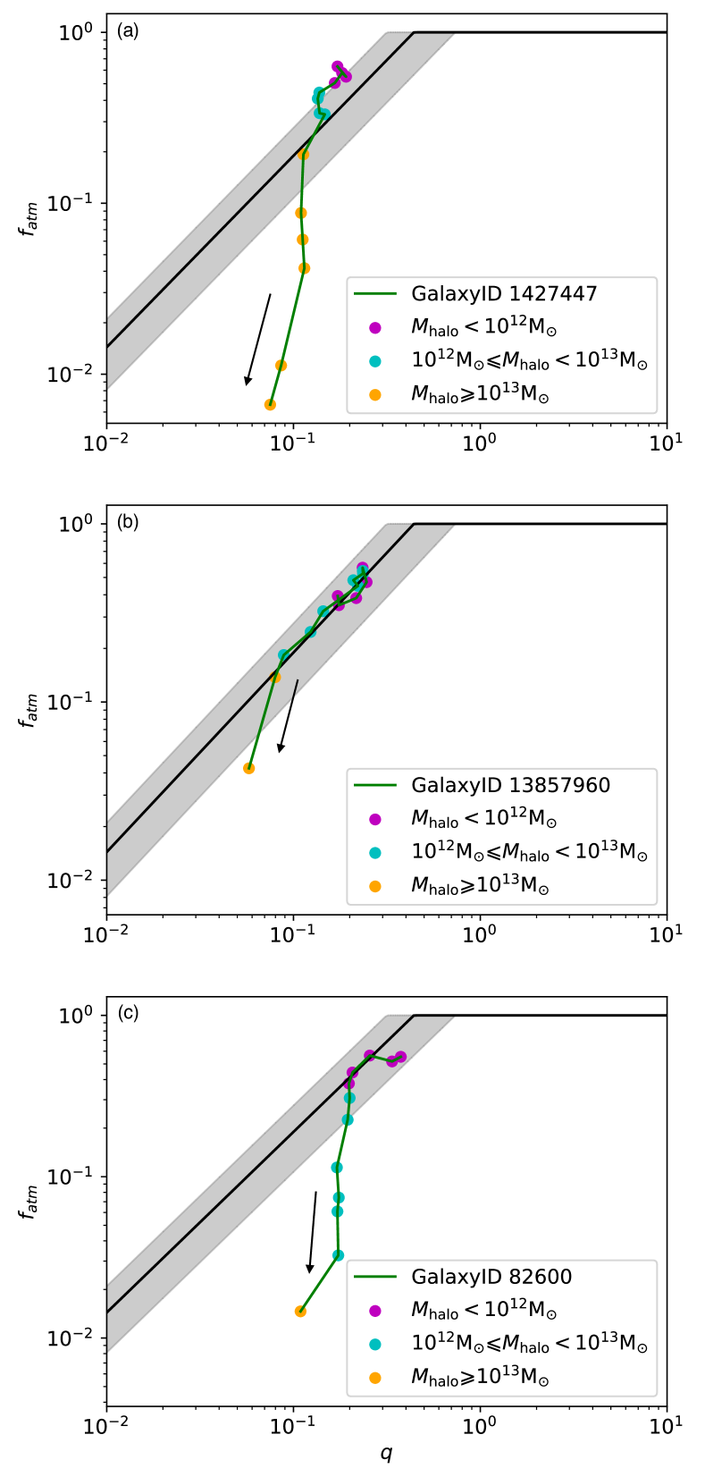
Figure 9: Three tracks of EAGLE galaxies in the $q-f_{\rm atm}$ plane from $z\approx 2$ to $z=0$. Arrows show the direction of time. The colours of the points represent the mass of the parent halo. The top and middle panels show the stripped satellite galaxies in our sample (heavily stripped+less stripped, 92% in total), while bottom panel shows rarer cases of pre-processing ($\sim$8%) in haloes with $M_{\rm halo}<10^{13}\rm M_{\odot}$.

4.3 Tracing the H i evolution history of cluster galaxies

Part of the reason for the large scatter in the simulated distance–$\Delta f_{q}$ relation (Figure 8) is that satellite galaxies with similar distances to their cluster centres have different histories. To understand the variety of these histories, we traced the satellite galaxies identified at $z=0$ back in time to redshift $z=2$ or to the highest redshift where the galaxy’s stellar mass lies still above the resolution limit ($10^{9}\rm M_{\odot}$). This provides a maximum of 13 snapshots per galaxy. In order to trace the infall history, we only retain the galaxies that have lived in a smaller halo ($<10^{13}\rm M_{\odot}$) before entering the cluster. Of our 117 cluster galaxies (in EAGLE FoFs $>10^{14}\rm M_{\odot}$), 113 (97%) satisfy this selection criterion. We refer to this sample of 113 galaxies with resolved histories as ‘Sample 1’.

The time interval between snapshots is $\approx 0.5-1$ Gyr, depending on the snapshot (see McAlpine et al., 2016). We use the merger trees from Qu et al. (2017), which are available in the public database, to reconstruct the history of the satellite galaxies. In addition, we record the halo mass, stellar mass, the H i mass from Lagos et al. (2015) and the sAM from Lagos et al. (2017) for each galaxy at different redshifts, from which we can reconstruct their $q$ and $f_{\rm atm}$ histories.

Sample 1 has been designed to have a very similar selection to the VIVA sample, while also allowing to track the galaxies back in time. However, with only 113 galaxies, this sample has limited statistical power. In order to increase the statistical power of the evolution analysis, we also consider a second sample (‘sample 2’), in which the minimum limit for the final halo mass at $z=0$ has been reduced from $10^{14}\rm M_{\odot}$ to $10^{13}\rm M_{\odot}$.This change increases the sample size to 690, while likely maintaining ram pressure stripping as the most significant source of H i deficiencies following the detailed analysis by Marasco et al. (2016). Note that Sample 1 is a subset of Sample 2.

Before presenting a statistical analysis of Sample 1 and 2, let us illustrate the evolution of some individual galaxies in the $q-f_{\rm atm}$ plane as they fall into a cluster. Figure 9 shows three such evolutionary tracks. In most cases, stripping starts occuring in haloes $>10^{13}\rm M_{\odot}$, as highlighted by the yellow colouring chosen for these haloes. We classify the evolutionary tracks into three classes, corresponding to the three panels in Figure 9. The first and second class (panels a and b) include all the galaxies that are not significantly H i deficient ($\Delta f_{q}<0.5$) before entering a halo more massive than $10^{13}\rm M_{\odot}$. In EAGLE, 90% (92%) of the galaxies fall into this category in Sample 1 (Sample 2). The difference between the first and second class lies in the final H i deficiency at $z=0$. The first class (panel a) contains all the strongly stripped cases ($\Delta f_{q}>0.5$ at $z=0$); the second class (panel b) contains all the weakly stripped cases ($\Delta f_{q}<0.5$ at $z=0$). In EAGLE, 52% (49%) fall into the first class; 38% (43%) fall into the second class. The most common reason for objects to fall into the second class is that they have not been long enough in a massive halo (e.g. only for 2 snapshots in Figure 9b). The remaining objects in the second class orbit the massive halo at large radii ($\gtrsim 0.8R_{200}$), where stripping is less effective. Finally, there is a third class of galaxies (panel c), which are already significantly H i deficient ($\Delta f_{q}>0.5$) before entering a massive halo ($>10^{13}\rm M_{\odot}$). These galaxies have been ‘pre-processed’ in a smaller galaxy group (typically between $10^{12}$ and $10^{13}\rm M_{\odot}$) prior to entering the massive halo. In EAGLE, 10% (8%) of the cluster galaxies fall into this category.

A way of representing the statistical evolution of $\Delta f_{q}$ of satellite galaxies from Sample 1 and Sample 2 is shown in Figure 10. This figure displays the histogram of $\Delta f_{q}$ in four different snapshots: immediately before entering a halo of $M_{\rm halo}>10^{13}\rm M_{\odot}$, refered as the snapshot $t-1$, the first snapshot after falling into such a halo (refered as the snapshot $t$), one snapshot later (refered as the snapshot $t+1$) and at $z=0$ (which mixes various relative times t, t+1,t+2…).

In Figure 10(a), the galaxies from Samples 1 and 2 exhibit a quite symmetric distribution in $\Delta f_{q}$ with a mean close to zero, showing that no significant H i deficiencies are seen, on average. The only statistically significant exception are a few systems in the positive tail at $\Delta f_{q}>0.5$, which correspond to pre-processed systems such as shown in Figure 9c.

At later times (panels (b)–(d)), the galaxies become increasingly H i deficient. The sparse snapshots in EAGLE limit a precise determination of when exactly the galaxies enter a cluster and how quickly their H i removal occurs. On average, the galaxies are 5–100-times H i deficient at $z=0$, i.e. their H i mass is 5–100 times smaller than the saturation mass (16- and 84-percentile range).

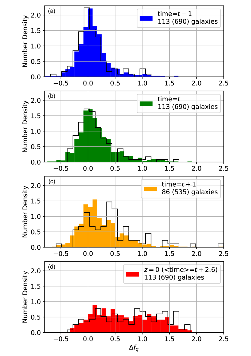
Figure 10: $\Delta f_{q}$ distributions of satellite galaxies in Sample 1 (black lines) and Sample 2 (filled histograms), defined in the 2nd paragraph of Section 4.3. The four panels represent four different snapshots, relative to the time the galaxies first enter their haloes with $M_{\rm halo}>10^{13}\rm M_{\odot}$ (details in Section 4.3). The number of galaxies are given in the legend for Sample 1 (Sample 2 in parentheses).

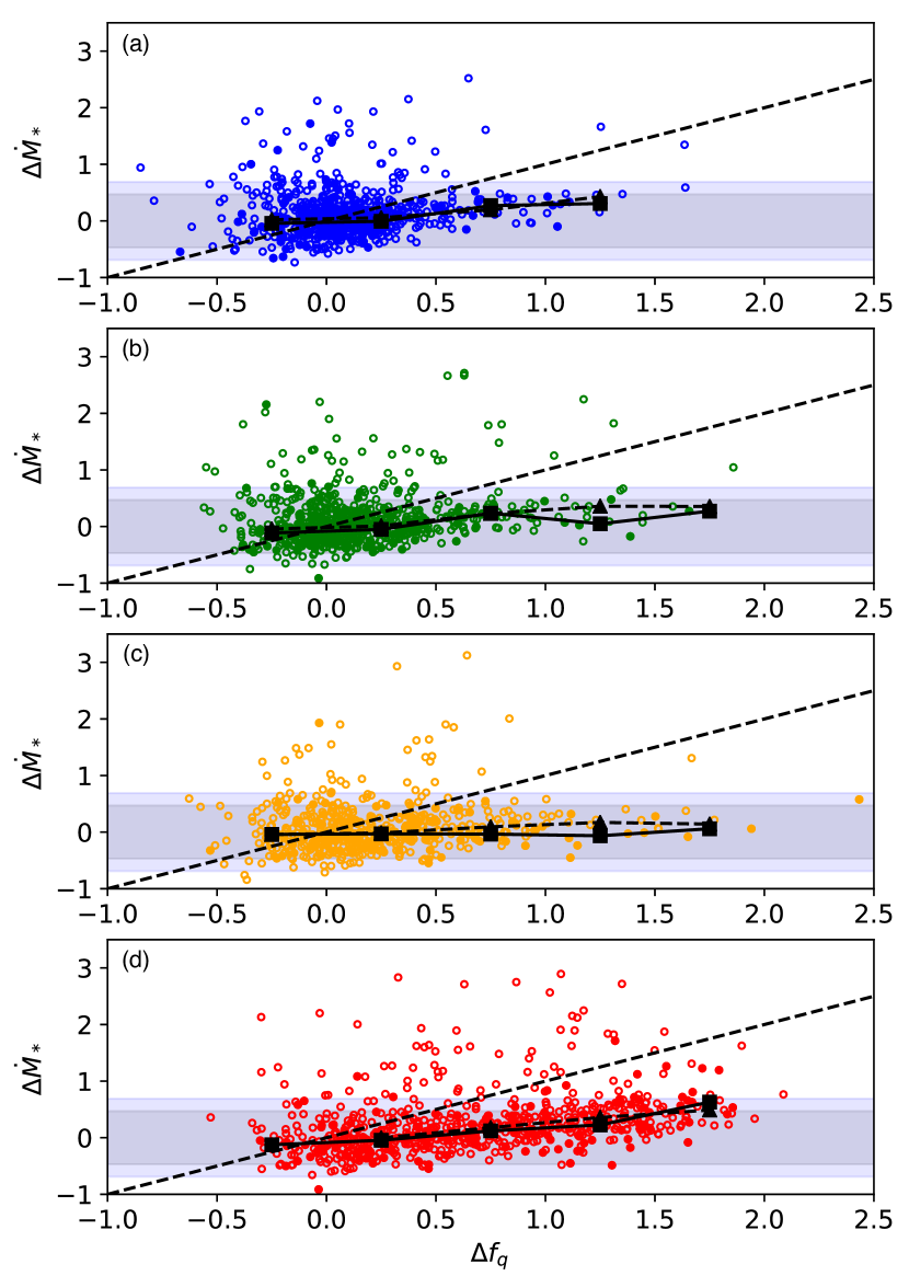
Figure 11: $\Delta f_{q}-\Delta\dot{M}_{*}$ relation of the galaxy sample for the same snapshots (relative to entering the cluster) shown in Figure 10. The solid points are Sample 1 and the empty points are Sample 2. The solid line shows the median value of sample 1 and the dashed line for sample 2. Light and dark grey shaded regions represent 1/5 to 5 and 1/3 to 3 factors below and above the SF main sequence, respectively. These factors are commonly used in the literature to define the SF main sequence width (Béthermin et al., 2015). The black squares and lines show the mean value of $\Delta\dot{M}_{*}$ in bins of $\Delta f_{q}$.

4.4 Discussion of quenching process of EAGLE cluster galaxies

Let us finally discuss the link between the H i deficiency estimator $\Delta f_{q}$ and the suppression of star formation. Observations (e.g. Cortese & Hughes, 2009; Boselli et al., 2014a) present a tight relation between the specific star formation rates and traditional H i deficiency parameters, indicating that the removal of gas changes faster than the quenching of the star formation activity. In hydrodynamic simulations and semi-analytic models, galaxies with suppressed star formation (SF) are typical also very H i poor or even have a complete absence of gas (Lagos et al., 2014; Marasco et al., 2016; Crain et al., 2017; Lagos et al., 2018; Stevens et al., 2019, among ohters). Among the physical processes behind this relation are galaxy-galaxy encounters (Marasco et al., 2016), ram pressure stripping (Stevens et al., 2019), strangulation (Lagos et al., 2018).

Here, we define the amount of relative suppression of star formation as the offset of a galaxy from the ‘main sequence’, i.e. the mean $M_{*}$–$\dot{M}_{*}$ relation at the considered redshift. The offset is measured in logarithmic units along the $\dot{M}_{*}$-axis,

$$\Delta\dot{M}_{*}={\log_{10}(\dot{M}_{*}^{\rm MS})}-{\log_{10}(\dot{M}_{*}^{\rm gal})},$$ (12)

where the reference value $\dot{M}_{*}^{\rm MS}$ is drawn from a redshift-dependent power-law fit to the $M_{*}$–$\dot{M}_{*}$ relation, for the subsample of galaxies with stellar masses between $10^{9}\rm M_{\odot}$ and $10^{10.5}\rm M_{\odot}$ and with specific star-formation rates (${\rm sSFR}=\dot{M}_{*}/M_{*}$) whose $\log_{10}({\rm sSFR}/[{\rm Gyr^{-1}}])\geqslant-2+0.5z$. This sSFR cut (for $z<2$) was proposed by Furlong et al. (2015) for the EAGLE simulations to exclude passive galaxies from the fit.

In other words, we fit the main sequence to EAGLE galaxies that are considered as star-forming at their redshift, as Eq. 13 shows, and we use this fit to estimate the distance to the main sequence for individual galaxies.

$$\log_{10}\left(\frac{\rm sSFR_{\rm MS}}{\rm Gyr}\right)=-0.14\times\log_{10}\frac{M_{*}}{\rm M_{\odot}}-0.47$$ (13)

The evolution of the star firmation main sequence as a function of redshift in EAGLE is similar to the observations (see Fig. 7 in Furlong et al., 2015), following the power law $(z+1)^{n}$ with $n\sim 3.5$.

Figure 11 presents the $\Delta f_{q}-\Delta\dot{M}_{*}$ relation for the same snapshots (relative to entering the cluster) as shown in Figure 10. The two samples present a similar trend.

When the gas is removed ($\Delta f_{q}$ becomes positively skewed), galaxies suppress their SFR moderately ($\Delta\dot{M}_{*}$ becomes larger) compared to their decrease in H i content, which may indicate the time delay between quenching and removal of H i gas. An important part of this delay is that the H i is stripped preferentially in the galactic outskirts, where the H i depletion time can be much longer than on average. Thus, removing this outer H i only has a weak effect star formation.

Interestingly, the $\Delta f_{q}$–$\Delta\dot{M}_{*}$ is not a one-to-one relation, in that the relative amount of SF suppression is smaller than the H i deficiency, irrespective of how long ago the suppression started. This finding is qualitatively consistent with observations in the range of $\Delta f_{q}<1$ (e.g. Cortese & Hughes, 2009) and explainable by the fact that stripping preferentially acts on the low-density outskirts of galactic disks, where the specific star formation rates of H i are very low. Removing this H i only implies a relatively small effect on star-formation. However, in heavily stripped systems ($\Delta f_{q}>1$), the results of observations and our simulated sample are in tension. Cortese & Hughes (2009); Boselli et al. (2014b) showed that when $\Delta f_{D}>1$ (which is similar to $\Delta f_{q}$), few galaxies are still in the SF main sequence while most of them are quenched. In our comparison sample (Sample 1), however, many galaxies are still on the SF main sequence despite them having $\Delta f_{q}>1$. It remains unclear how significant this tension is since the empirical evidence is subject to small number statistics and the EAGLE simulation is pushed to its mass resolution limit. Therefore, the $\Delta f_{q}-\Delta\dot{M}_{*}$ relation is an interesting topic for future investigations.

A direct comparison of the slope in the $\Delta f_{q}$–$\Delta\dot{M}_{*}$ between different models is not straight forward. For instance Figure 8 of Stevens et al. (2019) shows that $\Delta\dot{M}_{*}$ and $\Delta f_{q}$ covary, but a direct comparison to our study is complicated by different analysis techniques. A comparison of the $\Delta f_{q}$–$\Delta\dot{M}_{*}$ between models and observations could offer an interesting avenue for future research, which might benefit from the use of $\Delta f_{q}$ as a uniform definition of H i deficiencies.

5 Conclusions

In this paper, we analysed the H i deficiencies of environmentally affected cluster galaxies in the theoretical framework of the $(q,f_{\rm atm})$-plane, where $q$ is the atomic stability parameter introduced by O16. Field disk galaxies lie on a tight relation in this plane, which matches the analytically predicted relation for H i-saturated exponential disks. The offset $\Delta f_{q}$ from this relation is thus a sensible definition of a galaxy’s H i deficiency accounting for its baryonic mass and sAM, i.e. its major dynamical properties.

By applying $\Delta f_{q}$ to the galaxies in the VIVA survey, we confirmed the validity of $\Delta f_{q}$ as a sensitive probe of environmental removal/suppression of H i (e.g. due to stripping). In doing so, the $q$-values of the VIVA galaxies were computed using angular momentum measurements from spatially resolved kinematic 21cm data. By calculating $\Delta f_{q}$ for cluster galaxies in the EAGLE simulation, we confirmed that this simulation exhibits a qualitatively similar trend of H i-deficiencies as a function of cluster-centric distance, although a more quantitative comparison would require more than one observed cluster. The simulation allowed us to trace stripped galaxies back in time and determine the moment when the H i deficiencies first become detectable. Trough a statistical analysis of 690 galaxies in haloes more massive than $10^{13}\rm M_{\odot}$, we found that the $\Delta f_{q}$ distribution morphs significantly (towards positive values) as soon as the galaxies first enter the virial sphere of a halo more massive than $10^{13}\rm M_{\odot}$. This is paralleled by a slightly delayed quenching in the star-formation activity.

Compared to standard non-kinematic empirical definitions of H i deficiencies (such as the stellar mass based $\Delta f_{M}$, or the optical size+morphology based $\Delta f_{D}$), $\Delta f_{q}$ exhibits a list of interesting advantages: (1) it has a direct physical interpretation in terms of the H i saturation point; (2) In the case of disk-dominated systems, $\Delta f_{q}$ does not require any calibration to a reference sample of field galaxies, although we used such a reference sample to demonstrate that $\Delta f_{q}\approx 0$ in this case; (3) $\Delta f_{q}$ can be measured in observations and simulations in a like-to-like way. These advantages come at the prize of requiring kinematic data, ideally kinematic maps with $\lesssim 1\leavevmode\nobreak\ \rm kpc$ spatial and $\lesssim 10\leavevmode\nobreak\ \rm km/s$ velocity resolution in the rest-frame.

With the fast rise of integral field spectroscopy surveys (e.g. SAMI, HECTOR, MANGA) and radio interferometry surveys of H i (e.g. WALLABY and DINGO) on the Australian Square Kilometre Array Pathfinder (ASKAP) will move the field of survey astronomy towards large galaxy samples with sufficient data for accurate mass and angular momentum measurements and hence good determinations of $\Delta f_{q}$. Data from these surveys, as well as unresolved H i data from optically complete alternative surveys (e.g. Catinella et al., 2018) will enable much more systematic analyses of galaxies in the $(q,f_{\rm atm})$-plane. These studies will allow testing detailed theoretical predictions emerging from cosmological simulations and semi-analytic models. For instance, Stevens et al. (2018), using the semi-analytic model DARK SAGE, qualitatively predicted the different $q$–$f_{\rm atm}$ distributions of galaxies, whose H i was removed by entirely different mechanisms, such as ram pressure stripping, minor mergers and quasar-mode feedback.

Acknowledgements

We thank for the useful discussion from Yannick Bahe, Pascal Elahi and Ivy Wong. We acknowledge the Virgo Consortium for making their simulation data available. The EAGLE simulations were performed using the DiRAC-2 facility at Durham, managed by the ICC, and the PRACE facility Curie based in France at TGCC, CEA, Bruyéresle-Chatel. DO and CL thank for support from the Australia Research Council Discovery Project 160102235. CL thanks funding from ASTRO 3D. LC and DO are recipients of Australian Research Council Future Fellowships (FT180100066 and FT190100083) funded by the Australian Government. Parts of this research were conducted by the Australian Research Council Centre of Excellence for All Sky Astrophysics in 3 Dimensions (ASTRO 3D), through project number CE170100013. We thank the anonymous referee for their insightful and constructive feedback.

Appendix A VIVA data with uncertainties

Figure 12 shows the $M-f_{\rm atm}$ relation for disk field galaxies. The scatter of this relation is much larger than that of the $q-f_{\rm atm}$ relation. The samples of Lutz et al. (2018) and Murugeshan et al. (2019) are H i extreme for their mass, but for their stability parameter $q$, their H i fractions are normal.

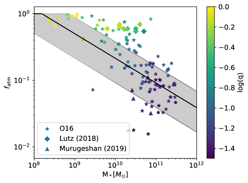
Figure 12: Disk mass vs. H i gas fraction, colored by parameter $q$. The samples are the same as in Figure 1. The black line shows the $M-f_{\rm atm}$ relation derived from the analytic model in Obreschkow et al. (2016). The shadow represents 68% of the predicted scatter in the spin parameter.

Figure 13 shows the $q$–$f_{\rm atm}$ relation of the VIVA data with log-normal statistical uncertainties plotted as error bars. The uncertainties of $q$ combine the uncertainties of estimating $M_{*}$ (Cortese et al., 2012), $j$ derived from Section 3 and a global 40% uncertainty of the H i velocity dispersion $\sigma$ (Obreschkow et al., 2016). The absolute uncertainties of $M_{\rm HI}$ and $M_{\rm H_{2}}$ are negligible compared to those of $M_{*}$. The uncertainty of $f_{\rm atm}$ includes those of $M_{*}$ (Cortese et al., 2012) and $M_{\rm HI}$ (Chung et al., 2009).

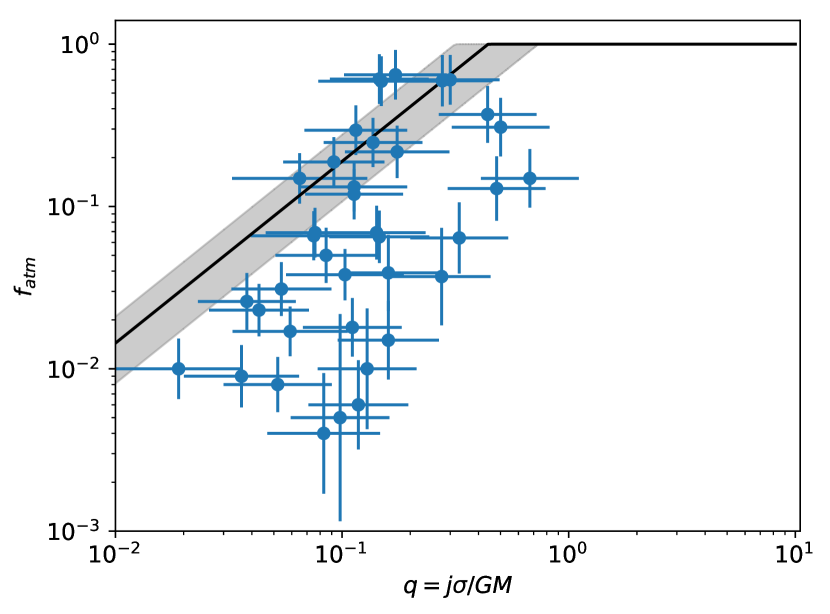
Figure 13: VIVA data in the $(q,f_{\rm atm})$-plane with log-normal uncertainties.

References

- Bahé et al. (2016) Bahé Y. M., et al., 2016, MNRAS, 456, 1115
- Béthermin et al. (2015) Béthermin M., et al., 2015, A&A, 573, A113
- Bolatto et al. (2013) Bolatto A. D., Wolfire M., Leroy A. K., 2013, ARA&A, 51, 207
- Boselli & Gavazzi (2006) Boselli A., Gavazzi G., 2006, PASP, 118, 517
- Boselli & Gavazzi (2009) Boselli A., Gavazzi G., 2009, A&A, 508, 201
- Boselli et al. (2014a) Boselli A., Cortese L., Boquien M., 2014a, A&A, 564, A65
- Boselli et al. (2014b) Boselli A., et al., 2014b, A&A, 570, A69
- Brown et al. (2015) Brown T., Catinella B., Cortese L., Kilborn V., Haynes M. P., Giovanelli R., 2015, MNRAS, 452, 2479
- Catinella et al. (2010) Catinella B., et al., 2010, MNRAS, 403, 683
- Catinella et al. (2018) Catinella B., et al., 2018, MNRAS, 476, 875
- Chung et al. (2009) Chung A., van Gorkom J. H., Kenney J. D. P., Crowl H., Vollmer B., 2009, AJ, 138, 1741
- Cortese & Hughes (2009) Cortese L., Hughes T. M., 2009, MNRAS, 400, 1225
- Cortese et al. (2011) Cortese L., Catinella B., Boissier S., Boselli A., Heinis S., 2011, MNRAS, 415, 1797
- Cortese et al. (2012) Cortese L., et al., 2012, A&A, 544, A101
- Cortese et al. (2016) Cortese L., et al., 2016, MNRAS, 463, 170
- Crain et al. (2015) Crain R. A., et al., 2015, MNRAS, 450, 1937
- Crain et al. (2017) Crain R. A., et al., 2017, MNRAS, 464, 4204
- Dalla Vecchia & Schaye (2012) Dalla Vecchia C., Schaye J., 2012, MNRAS, 426, 140
- Davies & Lewis (1973) Davies R. D., Lewis B. M., 1973, MNRAS, 165, 231
- Davies et al. (2019) Davies L. J. M., et al., 2019, MNRAS, 483, 5444
- Davis et al. (1985) Davis M., Efstathiou G., Frenk C. S., White S. D. M., 1985, ApJ, 292, 371
- Džudžar et al. (2019) Džudžar R., et al., 2019, MNRAS, 483, 5409
- Faber & Gallagher (1976) Faber S. M., Gallagher J. S., 1976, ApJ, 204, 365
- Faucher-Giguère et al. (2015) Faucher-Giguère C.-A., Hopkins P. F., Kereš D., Muratov A. L., Quataert E., Murray N., 2015, MNRAS, 449, 987
- Ford et al. (2013) Ford A. B., Oppenheimer B. D., Davé R., Katz N., Kollmeier J. A., Weinberg D. H., 2013, MNRAS, 432, 89
- Furlong et al. (2015) Furlong M., et al., 2015, MNRAS, 450, 4486
- Giovanelli & Haynes (1985) Giovanelli R., Haynes M. P., 1985, ApJ, 292, 404
- Gunn & Gott (1972) Gunn J. E., Gott III J. R., 1972, ApJ, 176, 1
- Haynes & Giovanelli (1984) Haynes M. P., Giovanelli R., 1984, AJ, 89, 758
- Haynes et al. (2000) Haynes M. P., Jore K. P., Barrett E. A., Broeils A. H., Murray B. M., 2000, AJ, 120, 703
- Hopkins et al. (2006) Hopkins P. F., Hernquist L., Cox T. J., Di Matteo T., Robertson B., Springel V., 2006, ApJ Sup., 163, 1
- Huang et al. (2012) Huang S., Haynes M. P., Giovanelli R., Brinchmann J., 2012, ApJ, 756, 113
- Krumholz (2013) Krumholz M. R., 2013, MNRAS, 436, 2747
- Lagos et al. (2011) Lagos C. D. P., Baugh C. M., Lacey C. G., Benson A. J., Kim H.-S., Power C., 2011, MNRAS, 418, 1649
- Lagos et al. (2014) Lagos C. d. P., Davis T. A., Lacey C. G., Zwaan M. A., Baugh C. M., Gonzalez-Perez V., Padilla N. D., 2014, MNRAS, 443, 1002
- Lagos et al. (2015) Lagos C. d. P., et al., 2015, MNRAS, 452, 3815
- Lagos et al. (2017) Lagos C. d. P., Theuns T., Stevens A. R. H., Cortese L., Padilla N. D., Davis T. A., Contreras S., Croton D., 2017, MNRAS, 464, 3850
- Lagos et al. (2018) Lagos C. d. P., Tobar R. J., Robotham A. S. G., Obreschkow D., Mitchell P. D., Power C., Elahi P. J., 2018, MNRAS, 481, 3573
- Leroy et al. (2008) Leroy A. K., Walter F., Brinks E., Bigiel F., de Blok W. J. G., Madore B., Thornley M. D., 2008, AJ, 136, 2782
- Lutz et al. (2018) Lutz K. A., et al., 2018, MNRAS,
- Maddox et al. (2015) Maddox N., Hess K. M., Obreschkow D., Jarvis M. J., Blyth S.-L., 2015, MNRAS, 447, 1610
- Marasco et al. (2016) Marasco A., Crain R. A., Schaye J., Bahé Y. M., van der Hulst T., Theuns T., Bower R. G., 2016, MNRAS, 461, 2630
- McAlpine et al. (2016) McAlpine S., et al., 2016, Astronomy and Computing, 15, 72
- Merritt (1983) Merritt D., 1983, ApJ, 264, 24
- Moore et al. (1996) Moore B., Katz N., Lake G., Dressler A., Oemler A., 1996, Nature, 379, 613
- Murugeshan et al. (2019) Murugeshan C., Kilborn V., Obreschkow D., Glazebrook K., Lutz K., Džudžar R., Dénes H., 2019, MNRAS, 483, 2398
- Obreschkow & Glazebrook (2014) Obreschkow D., Glazebrook K., 2014, ApJ, 784, 26
- Obreschkow et al. (2016) Obreschkow D., Glazebrook K., Kilborn V., Lutz K., 2016, ApJ Let., 824, L26
- Peng et al. (2015) Peng Y., Maiolino R., Cochrane R., 2015, Nature, 521, 192
- Qu et al. (2017) Qu Y., et al., 2017, MNRAS, 464, 1659
- Rahmati et al. (2013) Rahmati A., Schaye J., Pawlik A. H., Raičević M., 2013, MNRAS, 431, 2261
- Richings et al. (2014) Richings A. J., Schaye J., Oppenheimer B. D., 2014, MNRAS, 442, 2780
- Romanowsky & Fall (2012) Romanowsky A. J., Fall S. M., 2012, ApJ Sup., 203, 17
- Rosas-Guevara et al. (2015) Rosas-Guevara Y. M., et al., 2015, MNRAS, 454, 1038
- Schaye & Dalla Vecchia (2008) Schaye J., Dalla Vecchia C., 2008, MNRAS, 383, 1210
- Schaye et al. (2015) Schaye J., et al., 2015, MNRAS, 446, 521
- Stevens et al. (2018) Stevens A. R. H., Lagos C. d. P., Obreschkow D., Sinha M., 2018, MNRAS, 481, 5543
- Stevens et al. (2019) Stevens A. R. H., et al., 2019, MNRAS, 483, 5334
- Toomre (1964) Toomre A., 1964, ApJ, 139, 1217
- Walter et al. (2008) Walter F., Brinks E., de Blok W. J. G., Bigiel F., Kennicutt R. C., Thornley M. D., Leroy A., 2008, AJ, 136, 2563
- Wang et al. (2018) Wang L., et al., 2018, ApJ, 868, 93
- Wiersma et al. (2009a) Wiersma R. P. C., Schaye J., Smith B. D., 2009a, MNRAS, 393, 99
- Wiersma et al. (2009b) Wiersma R. P. C., Schaye J., Theuns T., Dalla Vecchia C., Tornatore L., 2009b, MNRAS, 399, 574
- Wright et al. (2018) Wright R. J., Lagos C. d. P., Davies L. J. M., Power C., Trayford J. W., Wong O. I., 2018, arXiv e-prints,
- van de Voort & Schaye (2012) van de Voort F., Schaye J., 2012, MNRAS, 423, 2991
- Jauzac, et al. (2016) Jauzac M., et al., 2016, MNRAS, 457, 2029
- Stroe, et al. (2015) Stroe A., et al., 2015, MNRAS, 450, 646
- Fall & Efstathiou (1980) Fall S. M., Efstathiou G., 1980, MNRAS, 193, 189
- Mo, Mao & White (1998) Mo H. J., Mao S., White S. D. M., 1998, MNRAS, 295, 319
- Gnedin & Kravtsov (2011) Gnedin N. Y., Kravtsov A. V., 2011, ApJ, 728, 88
- Urban, et al. (2011) Urban O., Werner N., Simionescu A., Allen S. W., Böhringer H., 2011, MNRAS, 414, 2101
- Ferrarese, et al. (2012) Ferrarese L., et al., 2012, ApJS, 200, 4
- McGaugh & Schombert (2015) McGaugh S. S., Schombert J. M., 2015, ApJ, 802, 18
- Romeo (2020) Romeo A. B., 2020, MNRAS, 491, 4843
- Romeo & Mogotsi (2018) Romeo A. B., Mogotsi K. M., 2018, MNRAS, 480, L23