Coarse-Graining of Microscopic Dynamics into
Mesoscopic Transient Potential Model

Abstract

We show that a mesoscopic coarse-grained dynamics model which incorporates the transient potential can be formally derived from an underlying microscopic dynamics model. As a microscopic dynamics model, we employ the overdamped Langevin equation. By utilizing the path probability and the Onsager-Machlup type action, we calculate the path probability for the coarse-grained mesoscopic degrees of freedom. The action for the mesoscopic degrees of freedom can be simplified by incorporating the transient potential. Then the dynamic equation for the mesoscopic degrees of freedom can be simply described by the Langevin equation with the transient potential (LETP). As a simple and analytically tractable approximation, we introduce additional degrees of freedom which express the state of the transient potential. Then we approximately express the dynamics of the system as the the combination of the LETP and the dynamics model for the transient potential. The resulting dynamics model has the same dynamical structure as the responsive particle dynamics (RaPiD) type models [W. J. Briels, Soft Matter 5, 4401 (2009)] and the multi-chain slip-spring type models [T. Uneyama and Y. Masubuchi, J. Chem. Phys. 137, 154902 (2012)]. As a demonstration, we apply our coarse-graining method with the LETP to a single particle dynamics in a supercooled liquid, and compare the results of the LETP with the molecular dynamics simulations and other coarse-graining models.

I Introduction

Soft matters such as polymers form various mesoscopic structures and exhibit various interesting dynamics. Coarse-grained models are useful to study the mesoscopic dynamics of such complex systems by simulations, especially at the long time scale. The coarse-graining reduces the degrees of freedom of the system, and changes the characteristic time and length scales. As a result, the computational costs required for simulations drastically reduce. For some soft matter systems such as polymer melts, due to their long relaxation times, we cannot study their long time relaxation behavior without coarse-grained modelsMüller-Plathe (2002); Padding and Briels (2011). Although the coarse-grained models are useful for simulations, the validity of simulation results are not always guaranteed. This is because the coarse-graining processes usually involve some approximations, and the validity of coarse-grained models strongly depends on the properties of the employed approximations. Unfortunately, the properties of approximations are not clear in some cases. Some coarse-grained models, such as the reptation model for entangled polymersDoi and Edwards (1986), are rather phenomenologically proposed, and not theoretically derived from the underlying microscopic models. For such cases, the relation between the microscopic models and mesoscopic coarse-grained models is not clear in general.

To study the properties of the coarse-grained models, theoretical methods based on statistical mechanics are useful. If the target system is not largely deviated from the equilibrium state, we can utilize the linear nonequilibrium statistical mechanics. The dynamic equations for coarse-grained degrees of freedom can be expressed, for example, as the Langevin equationItami and Sasa (2017) or the generalized Langevin equation (GLE)Kawasaki (1973). The transport coefficients can be related to the correlation functions of underlying microscopic dynamics, by the fluctuation-dissipation relationEvans and Morris (2008). The GENERIC (general equation for nonequilibrium reversible-irreversible coupling) formalism Grmela and Öttinger (1997); Öttinger and Grmela (1997); Español (2004) gives a general form of the effective dynamic equations. The theoretical analyses of the coarse-grained models from such view points are important to understand them in detail. For example, the dissipative particle dynamics (DPD), which was originally introduced phenomenologically, has been theoretically justified by using some statistical mechanical methodsEspañol and Warren (1995); Kinjo and Hyodo (2007); Español (2009).

For entangled polymer melts which exhibit characteristic slow relaxation behavior, various mesoscale phenomenological models have been proposed and utilizedDoi and Edwards (1986). Among them, some recently proposed models have interesting theoretical structures, from the view point of statistical mechanics. Kindt and Briels proposed the responsive particle dynamics (RaPiD) modelKindt and Briels (2007); Briels (2009, 2015), in which a single polymer chain is expressed as a single coarse-grained particle. In the RaPiD model, the number of entanglements between different polymer chains is employed as a fluctuating dynamical variable. The system is expressed by the particle positions and the numbers of entanglements between particles. Then the dynamics is described by the dynamic equations for the particles and the numbers of entanglements. Chappa et alChappa et al. (2012), and Uneyama and MasubuchiUneyama and Masubuchi (2012) proposed the multi-chain slip-spring (MCSS) model. In the MCSS model, polymer chains are modeled as Rouse chains, and chains are connected by so-called slip springs. The slip springs move along the chains, and are dynamically reconstructed at chain ends. In the MCSS model, the system is expressed by the positions of beads which construct polymer chains, and the states of slip-springs. The dynamics is described by the dynamic equation for beads and some stochastic transition rules for slip-springs.

The RaPiD and MCSS models have similar theoretical structures, and in fact, they can be unifiedUneyama (2019). The important point is that both the RaPiD and MCSS models employ some extra degrees of freedom (the numbers of entanglements or the slip spring states), in addition to the usual coarse-grained degrees of freedom (the positions of centers of mass or beads). If the system obeys the GLE, the state of the target system is fully described by the coarse-grained degrees of freedom. We may interpret that the thermodynamic state is uniquely determined by the coarse-grained degrees of freedom. In this sense, we may call the coarse-grained degrees of freeedom as the thermodynamic degrees of freedom. (The memory kernel does not affect the thermodynamic state and thus is qualitatively different from the thermodynamic degrees of freedom.) In the RaPiD and MCSS models, in contrast, the thermodynamic potential explicitly depends both on the coarse-grained and extra degrees of freedom. In this work, we may call such extra degrees of freedom as the “pseudo thermodynamic degrees of freedom”. The pseudo thermodynamic degrees of freedom dynamically modulate the effective potentials for the normal degrees of freedom. This dynamic modulation is realized through interaction potentials which are called the “transient potentials”Briels (2009, 2015). The success of the RaPiD and MCSS models leads us to an idea to generalize these models. If we can construct a general method which employs the transient potential and pseudo thermodynamic degrees of freedom, it will provide various mesoscopic coarse-grained dynamic equations for soft matter systems.

In this work, we show that we can actually construct a mesoscopic coarse-grained model with the transient potential, starting from the underlying microscopic dynamics model. In general, we cannot obtain the dynamic equation for the transient potential in an explicit form. We propose a simple dynamics model for the transient potential by using the pseudo thermodynamic degrees of freedom. We also propose some formal expressions for the dynamics of the transient potential. We show that, under some assumptions, we can derive the dynamic equation models which are consistent with the RaPiD and MCSS models. To study properties of our theoretical method in detail, we compare our method with the GLE and the Langevin equation with the fluctuating diffusivity. Also, we apply our model and the GLE to the dynamics of a single tagged particle in a supercooled liquid, and consider whether these coarse-graining methods can reasonably describe the dynamics or not.

II Theory

II.1 Microscopic Model

When we consider the coarse-graining, the Hamilton’s canonical equations are employed as microscopic models in most casesKawasaki (1973); Dengler . However, for soft matters such as polymers, the overdamped Langevin equations are reasonably utilized as the microscopic molecular modelsDoi and Edwards (1986). In addition, by applying the standard coarse-graining procedure, one can obtain a Langevin equation from the Hamilton’s canonical equations. Therefore, in this work, we employ an overdamped Langevin equation as the microscopic model. We consider the microscopic model which consists of $N$ particles in a three dimensional space, and we describe the position of the $i$-th particle as $\bm{r}_{i}$. We employ the following Langevin equation as the microscopic dynamic equation for the $i$-th particle:

$$\frac{d\bm{r}_{i}(t)}{dt}=-\sum_{j}\bm{L}_{ij}\cdot\frac{\partial U(\{\bm{r}_{i}(t)\})}{\partial\bm{r}_{i}(t)}+\sum_{j}\sqrt{2k_{B}T}\bm{B}_{ij}\cdot\bm{w}_{j}(t),$$ (1)

where $\bm{L}_{ij}$ is the mobility tensor, $U(\{\bm{r}_{i}\})$ is the interaction potential energy, $\bm{B}_{ij}$ is the noise coefficient tensor which satisfies $\bm{L}_{ij}=\sum_{k}\bm{B}_{ik}\cdot\bm{B}_{jk}^{\mathrm{T}}$ (the superscript “$\mathrm{T}$” represents the transpose), $k_{B}$ is the Boltzmann constant, $T$ is the temperature, and $\bm{w}_{i}(t)$ is the Gaussian white noise. From the Onsager’s reciprocal theorem, $\bm{L}_{ij}$ is a symmetric tensor. The noise $\bm{w}_{i}(t)$ should satisfy the following fluctuation-dissipation relation:

$$\langle\bm{w}_{i}(t)\rangle=0,\qquad\langle\bm{w}_{i}(t)\bm{w}_{j}(t^{\prime})\rangle=\bm{1}\delta_{ij}\delta(t-t^{\prime}),$$ (2)

where $\langle\dots\rangle$ is the statistical average and $\bm{1}$ is the unit tensor. Since eq (1) is a stochastic differential equation, we should specify the interpretation of the stochastic termGardiner (2004). We employ the Ito interpretation in this work. (One can employ the Stratonovich interpretation instead. In that case, we convert the Stratonovich type equation to the Ito type equationGardiner (2004). The result is the same in the current case.)

For the sake of simplicity, we introduce a short-hand notation for the positions as $\bm{R}\equiv[r_{1x},r_{1y},r_{1z},r_{2x},\dots,r_{Nz}]^{\mathrm{T}}$. The vector $\bm{R}$ can be interpreted as a $3N$-dimensional vector. We describe the mobility tensor, the noise coefficient tensor, and the Gaussian white noise in a similar way. For the sake of simplicity, we also employ the short-hand notation for the noise coefficient tensor, $\bm{B}=\bm{L}^{1/2}$. (Here, $\bm{L}^{1/2}$ represents the matrix square root which satisfies $\bm{L}^{1/2}\cdot(\bm{L}^{1/2})^{\mathrm{T}}=\bm{L}$.) Then, eq (1) can be rewritten as

$$\frac{d\bm{R}(t)}{dt}=-\bm{L}\cdot\frac{\partial U(\bm{R}(t))}{\partial\bm{R}(t)}+\sqrt{2k_{B}T}\bm{L}^{1/2}\cdot\bm{w}(t),$$ (3)

and eq (2) can be rewritten as

$$\langle\bm{w}(t)\rangle=0,\qquad\langle\bm{w}(t)\bm{w}(t^{\prime})\rangle=\bm{1}\delta(t-t^{\prime}).$$ (4)

In what follows, we use eq (3) as the microscopic dynamic equation. The equilibrium probability distribution for the position $\bm{R}$ is simply given as the Boltzmann distribution:

$$P_{\text{eq}}(\bm{R})=\frac{1}{\mathcal{Z}}\exp[-U(\bm{R})/k_{B}T],$$ (5)

where $\mathcal{Z}$ is the partition function:

$$\mathcal{Z}\equiv\int d\bm{R}\,\exp[-U(\bm{R})/k_{B}T].$$ (6)

For simplicity, we have assumed that all the particles in the system are distinguishable and ignored the Gibbs factor.

The probability (of the realization) for the Gaussian white noise which satisfies eq (4) is given asKleinert (2004)

$$\mathcal{P}[\bm{w}]=\mathcal{N}^{(\bm{w})}\exp\left[-\frac{1}{2}\int dt\,\bm{w}^{2}(t)\right],$$ (7)

where $\mathcal{N}^{(\bm{w})}$ is the normalization factor. Eq (7) can be interpreted as the probability of a specific path, and thus we may call it as the path probability. The normalization factor should be determined so that the functional integral (path integral) over $\bm{w}$ becomes unity: $\int\mathcal{D}\bm{w}\,\mathcal{P}[\bm{w}]=1$. (In this work, however, the normalization factor itself does not become important and thus we do not consider it in detail.) By combining eqs (3) and (7), the path probability for $\bm{R}(t)$ is given as

$$\mathcal{P}[\bm{R}]=\mathcal{N}^{(\bm{R})}\exp\left[-\mathcal{S}[\bm{R}]\right],$$ (8)

$$\mathcal{S}[\bm{R}]\equiv\frac{1}{2k_{B}T}\int dt\,G\left(\frac{d\bm{R}(t)}{dt}+\bm{L}\cdot\frac{\partial U(\bm{R}(t))}{\partial\bm{R}(t)};\bm{L}\right),$$ (9)

$$G(\bm{x},\bm{C})\equiv\frac{1}{2}\bm{x}^{\mathrm{T}}\cdot\bm{C}^{-1}\cdot\bm{x},$$ (10)

where $\mathcal{N}^{(\bm{R})}$ is the normalization factor (and is generally different from $\mathcal{N}^{(\bm{w})}$, due to the Jacobian for the variable transform), $\mathcal{S}[\bm{R}]$ is the action which gives the statistical weight for a specific path (the Onsager-Machlup action)Onsager and Machlup (1953); Machlup and Onsager (1953). In what follows, we express normalization factors for the path probabilities by $\mathcal{N}^{(\dotsb)}$ in a similar way. Eq (10) represents the Gaussian weight for a vector $\bm{x}$ and a covariance tensor $\bm{C}$. The covariance tensor $\bm{C}$ is a second rank symmetric positive definite tensor and $\bm{C}^{-1}$ is its inverse: $\bm{C}\cdot\bm{C}^{-1}=\bm{1}$. All the information on the microscopic dynamics is given by the path probability (8).

Before we consider the coarse-graining of the microscopic dynamic equation, here we briefly comment about the mobility model. In eq (3), the mobility tensor $\bm{L}$ is assumed to be independent of the position vector $\bm{R}(t)$. Such a situation is realized, for example, if we consider the situation where each particles feel the friction independently. The noise term is statistically independent of $\bm{R}(t)$ (the additive noise), and the analyses can be simplified. However, in general, the mobility tensor can depend on $\bm{R}(t)$, such as the case of the systems with the hydrodynamic interaction. If the mobility tensor depends on $\bm{R}(t)$, then the noise coefficient tensor $\bm{L}^{1/2}$ also depends on $\bm{R}(t)$. In such a case, the noise term becomes the multiplicative noise. The extension of our theory to the multiplicative noise is possible but complicated. (We show the extension in Appendix A.) Thus here we limit ourselves to the case of the additive noise.

II.2 Coarse-Graining

What we want to obtain here is the effective dynamic equation for some mesoscopic degrees of freedom. We limit ourselves that the mesoscopic degrees of freedom which can be given as the linear combinations the microscopic position, $\bm{R}(t)$. (The nonlinear variable transform can be employed but the calculation becomes complicated. We show the extension of the theory to the nonlinear variable transform in Appendix A.) For example, the centers of mass of molecules and the end-to-end vectors of polymers can be expressed as the linear combinations. We describe the $i$-th mesoscopic degrees of freedom as $Q_{i}$, and assume that there are $M$ mesoscopic variables. (The number of mesoscopic variables $M$ is generally much smaller than the number of microscopic degrees of freedom, $3N$.) Then, without loss of generality, we can transform the microscopic degrees of freedom $\bm{R}$ as

$$\bm{X}\equiv\begin{bmatrix}\bm{Q}\\ \bm{\theta}\end{bmatrix}=\bm{V}\cdot\bm{R},$$ (11)

where $\bm{Q}=[Q_{1},Q_{2},\dots,Q_{M}]^{\mathrm{T}}$ (an $M$-dimensional vector), $\bm{\theta}$ is a $(3N-M)$-dimensional vector, and $\bm{V}$ is a transformation matrix (of which dimension is $3N\times 3N$). We can take $\bm{\theta}$ so that the transformation matrix is invertible. Then we can express $\bm{R}$ as follows, by inverting eq (11):

$$\bm{R}=\bm{V}^{-1}\cdot\begin{bmatrix}\bm{Q}\\ \bm{\theta}\end{bmatrix}=\bm{V}^{-1}\bm{X}.$$ (12)

From eqs (11), a function of $\bm{R}$ such as the potential energy $U$ can be interpreted as a function of $\bm{X}$ (or, equivalently, a function of $\bm{Q}$ and $\bm{\theta}$).

We rewrite eqs (8) and (9) as functionals of $\bm{Q}$ and $\bm{\theta}$:

$$\mathcal{P}[\bm{Q},\bm{\theta}]=\mathcal{N}^{(\bm{Q},\bm{\theta})}\exp\left[-\mathcal{S}[\bm{Q},\bm{\theta}]\right],$$ (13)

$$\mathcal{S}[\bm{Q},\bm{\theta}]=\frac{1}{2k_{B}T}\int dt\,G\left(\frac{d\bm{X}(t)}{dt}+\bm{L}^{\prime}\cdot\frac{\partial U(\bm{X}(t))}{\partial\bm{X}(t)};\bm{L}^{\prime}\right),$$ (14)

where $\bm{L}^{\prime}\equiv\bm{V}\cdot\bm{L}\cdot\bm{V}^{-1}$ is the mobility tensor for $\bm{X}$. The path probability for the mesoscopic degrees of freedom can be obtained by eliminating the variable $\bm{\theta}$:

$$\mathcal{P}[\bm{Q}]=\int\mathcal{D}\bm{\theta}\,\mathcal{P}[\bm{Q},\bm{\theta}].$$ (15)

Unfortunately, $\bm{Q}$ and $\bm{\theta}$ are coupled in a complicated way. In general, we cannot evaluate eq (15) analytically. We need to introduce some approximations to proceed the calculation.

Here, we recall that the vector $\bm{\theta}$ can be arbitrarily chosen as long as $\bm{V}$ is invertible. Because we are interested only on the mesoscopic variable $\bm{Q}$, the choice of $\bm{\theta}$ is still rather arbitrarily at this stage. We choose $\bm{\theta}$ so that the action becomes a simple form. We employ $\bm{\theta}$ which gives the following mobility tensor

$$\bm{L}^{\prime}=\begin{bmatrix}\bm{\Lambda}&0\\ 0&\bm{M}\end{bmatrix},$$ (16)

where $\bm{\Lambda}$ and $\bm{M}$ are the mobility tensors for $\bm{Q}$ and $\bm{\theta}$, respectively. (The dimensions of $\bm{\Lambda}$ and $\bm{M}$ are $M\times M$ and $(3N-M)\times(3N-M)$, respectively.) In other words, we employ $\bm{\theta}$ which is $\bm{L}^{\prime}$-orthogonal to $\bm{Q}$:

$$\begin{bmatrix}\bm{Q}^{\mathrm{T}}&0\end{bmatrix}\cdot\bm{L}^{\prime}\cdot\begin{bmatrix}0\\ \bm{\theta}\end{bmatrix}=0.$$ (17)

With this specific choice of $\bm{\theta}$, we can further rewrite eq (14) as

$$\mathcal{S}[\bm{Q},\bm{\theta}]=\mathcal{S}^{(\bm{Q})}[\bm{Q}|\bm{\theta}]+\mathcal{S}^{(\bm{\theta})}[\bm{\theta}|\bm{Q}],$$ (18)

$$\mathcal{S}^{(\bm{Q})}[\bm{Q}|\bm{\theta}]\equiv\frac{1}{2k_{B}T}\int dt\,\left[G\left(\frac{d\bm{Q}(t)}{dt}+\bm{\Lambda}\cdot\frac{\partial U(\bm{Q}(t),\bm{\theta}(t))}{\partial\bm{Q}(t)};\bm{\Lambda}\right)\right],$$ (19)

$$\mathcal{S}^{(\bm{\theta})}[\bm{\theta}|\bm{Q}]\equiv\frac{1}{2k_{B}T}\int dt\,\left[G\left(\frac{d\bm{\theta}}{dt}+\bm{M}\cdot\frac{\partial U(\bm{Q}(t),\bm{\theta}(t))}{\partial\bm{\theta}(t)};\bm{M}\right)\right].$$ (20)

In eq (18), the Gaussian weight factor is split into two contributions (eqs (19) and (20)), unlike that in eq (14). However, it should be noticed that two split weight factors are coupled through the interaction potential $U(\bm{Q},\bm{\theta})$. Thus we cannot simply eliminate the degrees of freedom $\bm{\theta}$ by performing the functional integral over $\bm{\theta}$.

The Onsager-Machlup action (18) gives the statistical weight for a certain pathMartin et al. (1973). This is in analogy to the free energy functional in the field theoryOnuki (2002); the free energy functional gives the statistical weight for a certain field. In the field theory, we often introduce some auxiliary fields to obtain the approximate expression for the free energy. We expect that the action can be approximated in a similar way. We introduce a transient potential as an auxiliary variable. We interpret the potential at time $t$, $U(\bm{Q}(t),\bm{\theta}(t))$, as a transient potential $\Phi(\bm{Q}(t),t)$. This transient potential $\Phi$ is a function of $\bm{Q}$ and $t$, and is independent of $\bm{\theta}$. Following the standard procedure in the field theory Müller and Schmid (2005); Kawakatsu (2004), we use the following identity for the delta functional:

$$1=\int\mathcal{D}\Phi\,\delta\left[\Phi(\tilde{\bm{q}},t)-U(\tilde{\bm{q}},\bm{\theta}(t))\right].$$ (21)

Here, $\tilde{\bm{q}}$ represents the dummy variable which has the same dimension as $\bm{Q}$. By inserting eq (21) into eq (15), we have

$$\begin{split}\mathcal{P}[\bm{Q}]&=\int\mathcal{D}\bm{\theta}\mathcal{D}\Phi\,\delta\left[\Phi(\tilde{\bm{q}},t)-U(\tilde{\bm{q}},\bm{\theta}(t))\right]\mathcal{N}^{(\bm{Q},\bm{\theta})}\exp\left[-\mathcal{S}[\bm{Q},\bm{\theta}]\right]\\ &=\int\mathcal{D}\Phi\,\mathcal{N}^{(\bm{Q},\Phi)}\exp\left[-\tilde{\mathcal{S}}^{(\bm{Q})}[\bm{Q}|\Phi]\right]\tilde{\mathcal{P}}^{(\Phi)}[\Phi|\bm{Q}],\end{split}$$ (22)

$$\tilde{\mathcal{S}}^{(\bm{Q})}[\bm{Q}|\Phi]\equiv\frac{1}{2k_{B}T}\int dt\,G\left(\frac{d\bm{Q}(t)}{dt}+\bm{\Lambda}\cdot\frac{\partial\Phi(\bm{Q}(t),t)}{\partial\bm{Q}(t)};\bm{\Lambda}\right),$$ (23)

$$\begin{split}\tilde{\mathcal{P}}^{(\Phi)}[\Phi|\bm{Q}]&\equiv\int\mathcal{D}\bm{\theta}\,\delta\left[\Phi(\tilde{\bm{q}},t)-U(\tilde{\bm{q}},\bm{\theta}(t))\right]\\ &\qquad\times\exp\left[-\frac{1}{2k_{B}T}\int dt\,G\left(\frac{d\bm{\theta}}{dt}+\bm{M}\cdot\frac{\partial U(\bm{Q}(t),\bm{\theta}(t))}{\partial\bm{\theta}(t)};\bm{M}\right)\right].\end{split}$$ (24)

$\tilde{\mathcal{S}}^{(\bm{Q})}[\bm{Q}|\Phi]$ (eq (23)) can be interpreted as the action for $\bm{Q}$ under a given $\Phi$. Similarly, $\tilde{\mathcal{P}}^{(\Phi)}[\Phi|\bm{Q}]$ (eq (24)) can be interpreted as the path probability for $\Phi$ under a given $\bm{Q}$. For convenience, we introduce the action for $\Phi$ and rewrite eq (22) as

$$\mathcal{P}[\bm{Q}]=\int\mathcal{D}\Phi\,\mathcal{N}^{(\bm{Q},\Phi)}\exp\left[-\tilde{\mathcal{S}}^{(\bm{Q})}[\bm{Q}|\Phi]-\tilde{\mathcal{S}}^{(\Phi)}[\Phi|\bm{Q}]\right],$$ (25)

$$\tilde{\mathcal{S}}^{(\Phi)}[\Phi|\bm{Q}]\equiv-\ln\tilde{\mathcal{P}}^{(\Phi)}[\Phi|\bm{Q}].$$ (26)

So far, we have not introduced any approximations for the Onsager-Machlup action. Thus eq (25) is exactly equivalent to eq (15). Of course, eq (25) is just a formal expression and we have no simple analytic expression for the action $\tilde{\mathcal{S}}^{(\Phi)}$. Nonetheless eq (25) is useful for the coarse-graining. Eq (25) implies that, the transient potential $\Phi$ can be employed as additional degrees of freedom of the mesoscopic system. Instead of the path probability for $\bm{Q}$ (as eq (15)), here we consider the path probability for $\bm{Q}$ and $\Phi$:

$$\mathcal{P}[\bm{Q},\Phi]\equiv\mathcal{N}^{(\bm{Q},\Phi)}\exp\left[-\tilde{\mathcal{S}}^{(\bm{Q})}[\bm{Q}|\Phi]-\tilde{\mathcal{S}}^{(\Phi)}[\Phi|\bm{Q}]\right].$$ (27)

Clearly, we have $\int\mathcal{D}\Phi\mathcal{P}[\bm{Q},\Phi]=\mathcal{P}[\bm{Q}]$. Thus, if we eliminate the transient potential from eq (27), we recover the path probability for $\bm{Q}$. Now we have two actions in eq (27). The action for $\bm{Q}$, $\tilde{\mathcal{S}}^{(\bm{Q})}$ (eq (23)), is simple and we need no further manipulation for it (as long as $\Phi$ is given). The Langevin equation which corresponds to the action (23) is

$$\frac{d\bm{Q}(t)}{dt}=-\bm{\Lambda}\cdot\frac{\partial\Phi(\bm{Q}(t),t)}{\partial\bm{Q}(t)}+\sqrt{2k_{B}T}\bm{\Lambda}^{1/2}\cdot\bm{W}(t),$$ (28)

where $\bm{W}(t)$ is the $M$-dimensional Gaussian white noise vector. The noise $\bm{W}$ satisfies

$$\langle\bm{W}(t)\rangle=0,\qquad\langle\bm{W}(t)\bm{W}(t^{\prime})\rangle=\bm{1}\delta(t-t^{\prime}).$$ (29)

On the other hand, the action for $\Phi$, which is given by eqs (24) and (26), is not simple. From eq (26), the transient potential $\Phi$ obeys a stochastic time evolution equation (such as the Langevin equation), and this equation depends on $\bm{Q}$. We need to approximate it by a simple and tractable form, in order to obtain a dynamic equation model which is suitable for numerical simulations and theoretical analyses. Once we have the (approximate) dynamic equation for the transient potential, we can combine it with eq (28) to describe the dynamics of the mesoscopic degrees of freedom. Therefore, we find that the dynamics for the mesoscopic degrees of freedom is described by the Langevin equation with the transient potential (LETP). Eqs (27) and (28) formally justify the dynamics models with transient potentials, which were originally proposed as phenomenological models.

We can derive a similar Langevin equation for the cases where the noise is multiplicative and/or the variable transform is nonlinear. In general, the mobility tensor $\bm{\Lambda}$ becomes time-dependent and fluctuating quantity, just like the transient potential $\Phi$. The detailed calculations are shown in Appendix A. In what follows, for the sake of simplicity, we consider only the case of the additive noise and the linear variable transform.

II.3 Dynamics Model for Transient Potential

We should notice that our procedure in Sec. II.2 does not give the information on the dynamics of the transient potential. The derivation above is formal and one may criticize that it does not fully justify the LETP and thus cannot be accepted as a concrete derivation. Such a criticism is partly true. However, generally we cannot obtain the “exact” dynamic equations for coarse-grained systems. We need to employ some approximations for the full dynamics model to obtain a coarse-grained model, but approximations may not be fully justified and are rather empirical. In this subsection, we consider some methods to determine the effective dynamics model for the transient potential. We cannot determine the dynamics model uniquely, but we show that we can construct physically reasonable models under given approximations.

We start from a rather formal expression. The dynamics of the transient potential can be formally determined by the action $\tilde{\mathcal{S}}^{(\Phi)}[\Phi|\bm{Q}]$. From eq (27), we have

$$\tilde{\mathcal{S}}^{(\Phi)}[\Phi|\bm{Q}]=-\ln\mathcal{P}[\bm{Q},\Phi]-\tilde{\mathcal{S}}^{(\bm{Q})}[\bm{Q}|\Phi]+(\text{const.}).$$ (30)

The explicit form of the action $\tilde{\mathcal{S}}^{(\bm{Q})}[\bm{Q}|\Phi]$ is given by eq (23). Also, the path probability $\mathcal{P}[\bm{Q},\Phi]$ can be obtained as the ensemble average as:

$$\mathcal{P}[\bm{Q},\Phi]=\left\langle\delta(\bm{Q}(t)-\bm{Q}(\hat{\bm{R}}(t)))\,\delta[\Phi(\tilde{\bm{q}},t)-U(\tilde{\bm{q}},\bm{\theta}(\hat{\bm{R}}(t)))]\right\rangle^{(\hat{\bm{R}})}.$$ (31)

Here, $\hat{\bm{R}}$ represents a trajectory (or a path) directly generated by the Langevin equation (3), and the statistical average $\langle\dots\rangle^{(\hat{\bm{R}})}$ is taken for realizations of $\hat{\bm{R}}$. Therefore, in principle, we can construct the action $\tilde{\mathcal{S}}^{(\Phi)}[\Phi|\bm{Q}]$ from the path probability calculated by the direct microscopic simulations. Of course, the calculation of the path probability by eq (31) is practically impossible since the path probability is the joint distribution functional for the path and potential function in very high dimensions.

We consider to construct a dynamics model which can be used for practical simulations and analyses, by introducing some approximations. Even if the resulting dynamics model for the transient potential is not exact, the model which mimics the exact dynamics and gives physically reasonable results would be still useful. We assume that the transient potential can be approximately expressed as a function of a $Z$-dimensional auxiliary variable $\bm{A}(t)$:

$$\Phi(\tilde{\bm{q}},t)\approx\check{\Phi}(\tilde{\bm{q}},\bm{A}(t)).$$ (32)

The auxiliary variable $\bm{A}(t)$ should be chosen so that it gives a reasonable approximation for the dynamics of the transient potential. The dimension $Z$ should be sufficiently smaller than the dimension of $\bm{\theta}$, $Z\ll(3N-M)$. $\bm{A}(t)$ does not need to have the expression in terms of $\bm{\theta}(t)$. From eq (32), $\bm{A}(t)$ can be interpreted as a sort of the state of the transient potential. Then we expect that it behaves in a similar way to the coarse-grained variable $\bm{Q}(t)$. We further assume that, in equilibrium, the joint probability of $\bm{Q}$ and $\bm{A}$ should be expressed as

$$P_{\text{eq}}(\bm{Q},\bm{A})=\frac{1}{\check{\mathcal{Z}}}\exp[-\check{\Phi}(\bm{Q},\bm{A})/k_{B}T],$$ (33)

where $\check{\mathcal{Z}}$ is the effective partition function:

$$\check{\mathcal{Z}}=\int d\bm{Q}d\bm{A}\,\exp[-\check{\Phi}(\bm{Q},\bm{A})/k_{B}T].$$ (34)

Eq (33) is the same form as the usual partition function. Thus our assumption for $\bm{A}$ is that, it behaves as usual degrees of freedom. The thermodynamic state of the coarse-grained model is usually determined by the coarse-grained variable $\bm{Q}$. (As we stated, we may call such coarse-grained variables as the thermodynamic degrees of freedom, in this work.) In a similar way, we assume that the thermodynamic state can be now determined by $\bm{Q}$ and $\bm{A}$. Therefore we may call the auxiliary variable $\bm{A}$ as pseudo thermodynamic degrees of freedom.

Since the pseudo thermodynamic degrees of freedom were introduced to approximately describe the dynamics for the transient potential, they should never affect the equilibrium statistics of the mesoscopic degrees of freedom. Thus we require

$$P_{\text{eq}}(\bm{Q})=\int d\bm{A}\,P_{\text{eq}}(\bm{Q},\bm{A}),$$ (35)

or, equivalently,

$$\exp[-\mathcal{F}(\bm{Q})/k_{B}T]=\int d\bm{A}\,\exp[-\check{\Phi}(\bm{Q},\bm{A})/k_{B}T],$$ (36)

where $\mathcal{F}(\bm{Q})$ is the free energy for the mesoscopic degrees of freedom $\bm{Q}$:

$$\mathcal{F}(\bm{Q})\equiv-k_{B}T\ln\int d\bm{\theta}\exp[-U(\bm{Q},\bm{\theta})/k_{B}T].$$ (37)

From eq (36), we can relate the forces by the transient potential and the free energy as

$$\frac{\partial\mathcal{F}(\bm{Q})}{\partial\bm{Q}}=\int d\bm{A}\,\frac{\partial\check{\Phi}(\bm{Q},\bm{A})}{\partial\bm{Q}}P_{\text{eq}}(\bm{Q},\bm{A}).$$ (38)

The physical meaning of eq (38) is clear. If we average the thermodynamic force by the transient potential over the pseudo thermodynamic degrees of freedom, we just have the thermodynamic force by the free energy $\mathcal{F}$. Therefore, if the pseudo thermodynamic degrees of freedom relax much rapidly compared with the mesoscopic degrees of freedom, we just have a usual Langevin equation.

We want the dynamics model for $\bm{A}(t)$ to be simple and free from the memory kernel. We assume that $\bm{A}(t)$ obeys a Markovian stochastic process. We express the probability distribution of $\bm{Q}$ and $\bm{A}$ at time $t$ as $P(\bm{Q},\bm{A};t)$. For a Markovian process, the time evolution of $P(\bm{Q},\bm{A},t)$ can be formally expressed as follows.

$$\frac{\partial P(\bm{Q},\bm{A};t)}{\partial t} =[\mathcal{L}^{(\bm{Q})}+\mathcal{L}^{(\bm{A})}]P(\bm{Q},\bm{A};t),$$ (39)

$$\mathcal{L}^{(\bm{Q})}P(\bm{Q},\bm{A}) =\frac{\partial}{\partial\bm{Q}}\cdot\bm{\Lambda}\cdot\left[\frac{\partial\check{\Phi}(\bm{Q},\bm{A})}{\partial\bm{Q}}P(\bm{Q},\bm{A})+k_{B}T\frac{\partial P(\bm{Q},\bm{A})}{\partial\bm{Q}}\right],$$ (40)

$$\mathcal{L}^{(\bm{A})}P(\bm{Q},\bm{A}) =\int d\bm{A}^{\prime}\,[\check{\Omega}(\bm{A}|\bm{A}^{\prime},\bm{Q})P(\bm{Q},\bm{A}^{\prime})-\check{\Omega}(\bm{A}^{\prime}|\bm{A},\bm{Q})P(\bm{Q},\bm{A})].$$ (41)

Eq (40) is derived from the Langevin equation (28) with the approximate transient potential (32). $\check{\Omega}(\bm{A}^{\prime}|\bm{A},\bm{Q})$ is the transition rate from $\bm{A}$ to $\bm{A}^{\prime}$, and it should satisfy the detailed-balance condition:

$$\check{\Omega}(\bm{A}^{\prime}|\bm{A},\bm{Q})P_{\text{eq}}(\bm{Q},\bm{A})=\check{\Omega}(\bm{A}|\bm{A}^{\prime},\bm{Q})P_{\text{eq}}(\bm{Q},\bm{A}^{\prime}).$$ (42)

The dynamics of the coarse-grained system can be fully described by two hypothetically introduced functions $\check{\Phi}$ and $\check{\Omega}$. These functions can be interpreted as the trial functionsSchiff (1968). The optimal forms of these functions should be determined so that they minimize the differences between the approximate and exact dynamics. Therefore we can apply the variational methodSchiff (1968) to determine the functional forms of $\check{\Phi}$ and $\check{\Omega}$. The Kullback-Leibler divergenceKullback and Leibler (1951) would be suitable to measure how different two models areShell (2008); Español and Zúñiga (2011):

$$\mathcal{K}[\check{\Phi},\check{\Omega}]\equiv\int\mathcal{D}\bm{Q}\,\check{\mathcal{P}}[\bm{Q}|\check{\Phi},\check{\Omega}]\ln\frac{\check{\mathcal{P}}[\bm{Q}|\check{\Phi},\check{\Omega}]}{\mathcal{P}[\bm{Q}]},$$ (43)

where $\check{\mathcal{P}}[\bm{Q}|\check{\Phi},\check{\Omega}]$ and $\mathcal{P}[\bm{Q}]$ are the path probabilities for $\bm{Q}$ by the approximate and microscopic models. (The path probability by the approximate dynamics model can be interpreted as the functional of $\bm{Q},\check{\Phi}$, and $\check{\Omega}$.) The Kullback-Leibler divergence satisfies $\mathcal{K}[\check{\Phi},\check{\Omega}]\geq 0$ and it becomes zero ($\mathcal{K}[\check{\Phi},\check{\Omega}]=0$) if two path probabilities are the same. Therefore, by minimizing the Kullback-Leibler divergence with respect to trial functions, we have the most reasonable forms for $\check{\Phi}$ and $\check{\Omega}$. The most reasonable functional forms, $\check{\Phi}^{*}$ and $\check{\Omega}^{*}$, satisfy the following conditions:

$$\left.\frac{\delta\mathcal{K}[\check{\Phi},\check{\Omega}]}{\delta\check{\Phi}}\right|_{\check{\Phi}^{*},\check{\Omega}^{*}}=0,\qquad\left.\frac{\delta\mathcal{K}[\check{\Phi},\check{\Omega}]}{\delta\check{\Omega}}\right|_{\check{\Phi}^{*},\check{\Omega}^{*}}=0.$$ (44)

Unfortunately, the calculation of the path probabilities $\check{\mathcal{P}}[\bm{Q}|\check{\Phi},\check{\Omega}]$ and $\mathcal{P}[\bm{Q}]$ and the minimization with respect to $\check{\Phi}$ and $\check{\Omega}$ are still not practical. We will need further approximations and simplifications for the trial functions and the path probabilities. For example, we may assume the functional form and perform the minimization with respect to several parameters. We may approximate the path probabilities by the path probability for a single particle, or we may employ the hypothetical path probability forms based on dynamical quantities such as the mean-square displacement.

There are several possible simple yet non-trivial models for the dynamics of $\bm{A}$. Among them, the simplest model would be the following Langevin equation for $\bm{A}$:

$$\frac{d\bm{A}(t)}{dt}=-\bm{\Gamma}\cdot\frac{\partial\check{\Phi}(\bm{Q}(t),\bm{A}(t))}{\partial\bm{A}(t)}+\sqrt{2k_{B}T}\bm{\Gamma}^{1/2}\cdot\bm{\omega}(t).$$ (45)

Here, $\bm{\Gamma}$ is the mobility tensor and $\bm{\omega}$ is the $Z$-dimensional Gaussian white noise. As before, we have simply assumed that the mobility tensor $\bm{\Gamma}$ is independent of $\bm{Q}$ and $\bm{A}$. The fluctuation-dissipation relation should be satisfied for the noise $\bm{\omega}$:

$$\langle\bm{\omega}(t)\rangle=0,\qquad\langle\bm{\omega}(t)\bm{\omega}(t^{\prime})\rangle=\bm{1}\delta(t-t^{\prime}).$$ (46)

Eqs (28) and (45) give the dynamics which is consistent with eqs (41) and (42). This type of coupled Langevin equations correspond to the RaPiD model for entangled polymersKindt and Briels (2007); Briels (2009, 2015). We can employ other dynamics models, as well. For example, if the transient potential instantaneously changes, the simple transition dynamics models would be suitable. We may employ a specific transition rate model such as the Glauber dynamics. Then the transition rate will be explicitly given in terms of the difference of the transient potential before and after the transition. This type of coupling of the Langevin equation and transition dynamics corresponds to the MCSS modelUneyama and Masubuchi (2012) and the transient bond modelUneyama (2019) for entangled polymers, and the alternating diffusive state model for supercooled liquidsHachiya et al. (2019).

III Discussions

III.1 Generalized Langevin Equation

We have proposed the LETP model by introducing the transient potential to approximately describe the mesoscopic dynamics. Also, we have proposed some possible approximate dynamics model for the transient potential by introducing the pseudo thermodynamic degrees of freedom. This is not a unique way to describe the complex mesoscopic dynamics. We may employ other methods to describe the mesoscopic dynamics. The most popular and established way is to use the projection operatorKawasaki (1973); Dengler . The projection operator method gives the GLE as the effective dynamic equation for the mesoscopic degrees of freedom. The GLE involves the memory kernel which directly expresses the memory effect for the mesoscopic degrees of freedom. In this subsection, we compare the LETP model with the dynamic equation which incorporates the memory kernel.

We start from the same microscopic dynamics model as Sec. II, and consider the effective dynamic equation for the degrees of freedom $\bm{Q}$. By eliminating the fast degrees of freedom, we have the GLE as the dynamic equation for the mesoscopic degrees of freedom:

$$\frac{d\bm{Q}(t)}{dt}=-\int_{-\infty}^{t}dt^{\prime}\,\bm{K}(t-t^{\prime})\cdot\frac{\partial\mathcal{F}(\bm{Q}(t^{\prime}))}{\partial\bm{Q}(t^{\prime})}+\bm{\xi}(t),$$ (47)

where $\bm{K}(t)$ is the memory kernel and $\bm{\xi}(t)$ is the colored noise. The fluctuation-dissipation relation requires the noise to satisfy

$$\langle\bm{\xi}(t)\rangle=0,\qquad\langle\bm{\xi}(t)\bm{\xi}(t^{\prime})\rangle=k_{B}T\bm{K}(|t-t^{\prime}|).$$ (48)

The projection operator method gives eqs (47) and (48), but it does not tell us the detailed statistical properties of the colored noise $\bm{\xi}(t)$. In most practical cases, the colored noise $\bm{\xi}(t)$ is simply assumed to be Gaussian. (This assumption seems to be often employed implicitly.) Then the dynamic equation for the mesoscopic degrees of freedom can be fully specified. This Gaussian assumption cannot be justified a priori, and we should interpret it as an approximation. In this work, we explicitly distinguish the GLE with the Gaussian noise (GLEG) with the GLE with a general non-Gaussian noise. It would be reasonable to consider that both the GLEG and the LETP can be obtained from the same microscopic dynamics model with different approximations. We expect that the difference between the GLEG and the LETP originates from the properties of the employed approximations.

To consider the difference between the GLEG and the LETP in detail, it would be better for us to derive the GLEG by utilizing the path probability and the Onsager-Machlup action. Therefore here we go back to eqs (13) and (18). As we mentioned, two actions in eq (18) are coupled via the interaction potential $U(\bm{Q},\bm{\theta})$. In the derivation of the LETP, we introduced the transient potential to rewrite the action for $\bm{Q}$ in a simple form. Here we consider to introduce a different quantity to simplify the action for $\bm{Q}$. We consider an average of the force term for $\bm{Q}$,

$$\bar{\bm{v}}[\bm{Q},t]=-\left\langle\bm{\Lambda}\cdot\frac{\partial U(\bm{Q}(t),\bm{\theta}(t))}{\partial\bm{Q}(t)}\right\rangle^{(\bm{\theta})},$$ (49)

where $\langle\dots\rangle^{(\bm{\theta})}$ represents the statistical average over $\bm{\theta}$. The thus defined $\bar{\bm{v}}$ can be interpreted as the average “velocity” for the mesoscopic degrees of freedom $\bm{Q}$. From the causality, $\bar{\bm{v}}$ at time $t$ is a functional of $\bm{Q}(t^{\prime})$ for $t^{\prime}\leq t$. If the system is fluctuating around the equilibrium, $\bar{\bm{v}}$ should be expressed as a linear function of the thermodynamic force. Thus we expect the following form for $\bar{\bm{v}}$:

$$\bar{\bm{v}}[\bm{Q},t]=-\int_{-\infty}^{t}dt^{\prime}\,\bm{K}(t-t^{\prime})\cdot\frac{\partial\mathcal{F}(\bm{Q}(t^{\prime}))}{\partial\bm{Q}(t^{\prime})}.$$ (50)

We may employ eq (50) as the definition of $\bar{\bm{v}}$, instead of eq (49). Anyway, $\bar{\bm{v}}$ is an average and the force term is fluctuating around it. We introduce the deviation of the force term from $\bar{\bm{v}}$ as $\Delta\bm{v}(t)$:

$$\Delta\bm{v}(t)=-\bm{\Lambda}\cdot\frac{\partial U(\bm{Q}(t),\bm{\theta}(t))}{\partial\bm{Q}(t)}-\bar{\bm{v}}[\bm{Q},t].$$ (51)

This $\Delta\bm{v}(t)$ can be interpreted as the fluctuation around the reference path. As before, we utilize the functional identity to introduce $\Delta\bm{v}$ as additional degrees of freedom:

$$1=\int\mathcal{D}\Delta\bm{v}\,\delta\left[\Delta\bm{v}(t)-\bm{\Lambda}\cdot\frac{\partial U(\bm{Q}(t),\bm{\theta}(t))}{\partial\bm{Q}(t)}-\bar{\bm{v}}[\bm{Q},t]\right].$$ (52)

We insert eq (52) into eq (13). Then we can rewrite the path probability for $\bm{Q}$ as

$$\begin{split}\mathcal{P}[\bm{Q}]&=\int\mathcal{D}\bm{\theta}\mathcal{D}\Delta\bm{v}\,\delta\left[\Delta\bm{v}(t)-\bm{\Lambda}\cdot\frac{\partial U(\bm{Q}(t),\bm{\theta}(t))}{\partial\bm{Q}(t)}-\bar{\bm{v}}[\bm{Q},t]\right]\mathcal{N}^{(\bm{Q},\bm{\theta})}\exp\left[-\mathcal{S}[\bm{Q},\bm{\theta}]\right]\\ &=\int\mathcal{D}\Delta\bm{v}\,\mathcal{N}^{(\bm{Q},\Delta\bm{v})}\exp\left[-\bar{\mathcal{S}}^{(\bm{Q})}[\bm{Q}|\Delta\bm{v}]-\bar{\mathcal{S}}^{(\Delta\bm{v})}[\Delta\bm{v}|\bm{Q}]\right],\end{split}$$ (53)

with

$$\bar{\mathcal{S}}^{(\bm{Q})}[\bm{Q}|\Delta\bm{v}]\equiv\frac{1}{2k_{B}T}\int dt\,G\left(\frac{d\bm{Q}(t)}{dt}-\bar{\bm{v}}[\bm{Q},t]-\Delta\bm{v}(t);\bm{\Lambda}\right),$$ (54)

$$\begin{split}\bar{\mathcal{S}}^{(\Delta\bm{v})}[\Delta\bm{v}|\bm{Q}]&\equiv-\ln\int\mathcal{D}\bm{\theta}\,\delta\left[\Delta\bm{v}(t)-\bm{\Lambda}\cdot\frac{\partial U(\bm{Q}(t),\bm{\theta}(t))}{\partial\bm{Q}(t)}-\bar{\bm{v}}[\bm{Q},t]\right]\\ &\qquad\times\exp\left[-\frac{1}{2k_{B}T}\int dt\,G\left(\frac{d\bm{\theta}(t)}{dt}+\bm{M}\cdot\frac{\partial U(\bm{Q}(t),\bm{\theta}(t))}{\partial\bm{\theta}(t)};\bm{M}\right)\right],\end{split}$$ (55)

where $\mathcal{N}^{(\bm{Q},\Delta\bm{v})}$ is the normalization factor. Eqs (53)-(55) have similar forms to eqs (22)-(26). As the case of eqs (22)-(26), eqs (53)-(55) are derived without approximations and thus they are formally exact.

To obtain the GLEG, we approximate the action for $\Delta\bm{v}$ (eq (55)) by a simple Gaussian form:

$$\bar{\mathcal{S}}^{(\Delta\bm{v})}[\Delta\bm{v}|\bm{Q}]\approx-\frac{1}{2k_{B}T}\int dtdt^{\prime}\,\Delta\bm{v}^{\mathrm{T}}(t)\cdot\bar{\bm{C}}^{-1}(t-t^{\prime})\cdot\Delta\bm{v}(t^{\prime}),$$ (56)

where $\bar{\bm{C}}(t)$ is a tensor which represents the covariance of $\Delta\bm{v}$. (The explicit form of this tensor is not required here.) Under this approximation, the path probability for $\bm{Q}$ can be explicitly calculated. The Gaussian weight for $\bm{Q}$ in eq (54) can be also interpreted as a Gaussian weight for $\Delta\bm{v}$. Thus the path probability for $\bm{Q}$ can be calculated by integrating the path probability over $\Delta\bm{v}$. From eqs (53),  (54), and (56), we have

$$\begin{split}\mathcal{P}[\bm{Q}]&\approx\int\mathcal{D}\Delta\bm{v}\,\mathcal{N}^{(\bm{Q},\Delta\bm{v})}\exp\bigg{[}-\frac{1}{2k_{B}T}\int dtdt^{\prime}\,\bigg{[}\Delta\bm{v}^{\mathrm{T}}(t)\cdot\bar{\bm{C}}^{-1}(t-t^{\prime})\cdot\Delta\bm{v}(t^{\prime})\\ &\qquad+\left(\Delta\bm{v}(t)-\frac{d\bm{Q}(t)}{dt}+\bm{v}[\bm{Q},t]\right)^{\mathrm{T}}\cdot 2\bm{\Lambda}\delta(t-t^{\prime})\cdot\left(\Delta\bm{v}(t^{\prime})-\frac{d\bm{Q}(t^{\prime})}{dt^{\prime}}+\bm{v}[\bm{Q},t^{\prime}]\right)\bigg{]}\bigg{]}\\ &=\mathcal{N}^{(\bm{Q})}\exp\bigg{[}-\frac{1}{2k_{B}T}\int dtdt^{\prime}\,\left(\frac{d\bm{Q}(t)}{dt}-\bm{v}[\bm{Q},t]\right)^{\mathrm{T}}\cdot\bar{\bm{K}}^{-1}(t-t^{\prime})\cdot\left(\frac{d\bm{Q}(t^{\prime})}{dt^{\prime}}-\bm{v}[\bm{Q},t^{\prime}]\right)\bigg{]},\end{split}$$ (57)

where $\mathcal{N}^{(\bm{Q})}$ is the normalization factor and $\bar{\bm{K}}(t)$ is the kernel function defined as

$$\bar{\bm{K}}(t)=\bar{\bm{C}}(t)+2\bm{\Lambda}\delta(t).$$ (58)

Eq (57) is equivalent to the GLEG if the kernel $\bar{\bm{K}}(t)$ is given as $\bar{\bm{K}}(t)=\bm{K}(|t|)$. This condition is equivalent to the fluctuation-dissipation relation (48), and thus it should be satisfied to reproduce the correct equilibrium distribution. Thus we find that the GLEG can be obtained from eqs (13) and (18), if we approximate the fluctuation of the force term $\Delta\bm{v}$ by a simple Gaussian from (eq (56)).

By comparing the derivations of the GLEG and the LETP, we find some differences between them. The first difference is that the LETP employs additional degrees of freedom, the transient potential, to express the force term in the action (18). The GLEG employs the average $\bar{\bm{v}}$, which is a functional of $\bm{Q}$, instead. This average $\bar{\bm{v}}$ incorporates the memory kernel. The second difference is that the additional degrees of freedom is not eliminated in the LETP. In other words, we explicitly have the dynamic equation for the additional degrees of freedom (the transient potential $\Phi$), in addition to that for the mesoscopic degrees of freedom $\bm{Q}$. This is in contrast to the case of the GLEG. To derive the GLEG, we eliminated the fluctuation around the average, $\Delta\bm{v}$, by integrating the path probability over it. The LETP does not require the memory kernel but requires additional degrees of freedom, whereas the GLEG does not require additional degrees of freedom but requires the memory kernel.

III.2 Example: Supercooled Liquid

Because the GLEG and the LETP are based on different approximations, some statistical properties of them can be quantitatively different, although the target system is the same. As a simple example, here we consider the effective dynamic equation model for a single tagged particle (or the center of mass of a tagged molecule) in a supercooled liquid in a three dimensional space.

The dynamics of supercooled liquids have been widely studied by binary Lennard-Jones mixture systemsKob and Andersen (1994, 1995a, 1995b); Yamamoto and Onuki (1998a, b); Kob (1999); Vorselaars et al. (2007). To study the diffusion behavior, the mean-square displacement (MSD) data are useful. If the temperature is sufficiently high, we just observe normal diffusion behavior: $\langle[\bm{r}(t)-\bm{r}(0)]^{2}\rangle\propto t$. If the temperature is sufficiently low, we observe the slowing-down of the dynamics. As a result, the MSD of the particle typically show three regionsHunter and Weeks (2012); Klix et al. (2015). At the short time region, it exhibits a normal diffusion. At the intermediate time region, the MSD becomes almost independent of time, and exhibits a plateau. At the long time region, it again exhibits a normal diffusion. Therefore, the MSD of a particle would be as follows:

$$\langle[\bm{r}(t)-\bm{r}(0)]^{2}\rangle\propto\begin{cases}t^{1}&(t\lesssim\tau^{\prime}),\\ t^{0}&(\tau^{\prime}\lesssim t\lesssim\tau^{\prime\prime}),\\ t^{1}&(\tau^{\prime\prime}\lesssim t),\end{cases}$$ (59)

where $\tau^{\prime}$ and $\tau^{\prime\prime}$ are characteristic time scales. (Strictly speaking, at sufficiently short time scale, we observe the ballistic diffusion behavior. In this work we consider overdamped dynamics and thus we do not consider the ballistic region.) The MSD data are not sufficient to characterize the dynamics of a particle. The distribution of the displacement is generally not Gaussian, and the non-Gaussianity cannot be detected via the MSD. The non-Gaussianity parameter (NGP)Rahman (1964); Vorselaars et al. (2007), which characterizes the deviation of the diffusion behavior from the ideal Gaussian behavior, is useful to study the non-Gaussianity. For a three dimensional system, the NGP is defined as $\alpha(t)\equiv 3\langle|\bm{r}(t)-\bm{r}(0)|^{4}\rangle/5\langle[\bm{r}(t)-\bm{r}(0)]^{2}\rangle^{2}-1$.

We show the MSD and NGP of a particle in a model binary Lennard-Jones mixture with different temperatures in Figure 1. Here, the dimensionless units are employed (the characteristic length, mass, and energy are set to be unity) and the temperature is changed from $k_{B}T=0.4$ to $k_{B}T=1$. The details of the simulation model and the simulation setup are shown in Appendix B. We show some trajectories of particles in a supercooled liquid at $k_{B}T=0.6$ in Figure 2. We clearly observe that the trajectories are qualitatively different from those of normal Brownian motions. This can be interpreted as the fluctuation of the mobility, which is called the dynamic heterogeneity.

We consider whether such behavior can be successfully modeled by the GLEG and the LETP. We express the position of the tagged particle as $\bm{r}(t)$, and use this as the mesoscopic degrees of freedom. We construct the effective dynamic equations for $\bm{r}$, and then analyze the MSD and NGP.

From the translational symmetry, the free energy is zero: $\mathcal{F}(\bm{r})=0$. Therefore, if we employ the GLEG to describe the dynamics, we have the dynamic equation as

$$\frac{d\bm{r}(t)}{dt}=\bm{\xi}(t),$$ (60)

where $\bm{\xi}(t)$ is the Gaussian colored noise. The first and second moments of the noise $\bm{\xi}(t)$ are

$$\langle\bm{\xi}(t)\rangle=0,\qquad\langle\bm{\xi}(t)\bm{\xi}(t^{\prime})\rangle=k_{B}TK(|t-t^{\prime}|)\bm{1}.$$ (61)

Here $K(t)$ is the (scalar) memory kernel. We have assumed that the system is isotropic and the memory kernel tensor is given as an isotropic tensor. The MSD is simply calculated to be

$$\langle[\bm{r}(t)-\bm{r}(0)]^{2}\rangle=\int_{0}^{t}dt^{\prime}\int_{0}^{t}dt^{\prime\prime}\,\langle\bm{\xi}(t^{\prime})\cdot\bm{\xi}(t^{\prime\prime})\rangle=6k_{B}T\int_{0}^{t}dt^{\prime}\,(t-t^{\prime})K(t^{\prime}).$$ (62)

Thus we find that the memory kernel can be determined if the MSD of the tagged particle is given. From the Gaussian nature of the noise $\bm{\xi}(t)$, the NGP is exactly zero: $\alpha(t)=0$. This means that, the GLEG can reproduce the MSD observed in supercooled liquids successfully (by tuning the memory kernel), but it cannot reproduce the non-Gaussian behavior.

If we employ the LETP, the dynamic equation becomes

$$\frac{d\bm{r}(t)}{dt}=-\Lambda\frac{\partial\check{\Phi}(\bm{r}(t),\bm{A}(t))}{\partial\bm{r}(t)}+\sqrt{2k_{B}T\Lambda}\bm{W}(t),$$ (63)

where $\Lambda$ is the (scalar) mobility and $\bm{W}(t)$ is the Gaussian white noise. The force term by the transient potential in eq (63) is not zero. Unlike the case of the GLEG, we should specify the dynamics model of the transient potential or the pseudo thermodynamic degrees of freedom. As a simple yet nontrivial model, we employ a simple harmonic type potential as the transient potential:

$$\check{\Phi}(\bm{r},\bm{A})=\frac{1}{2}\kappa(\bm{r}-\bm{A})^{2},$$ (64)

where $\kappa$ is the spring constant and $\bm{A}$ corresponds to the center position of the potential. (The dimension of $\bm{A}$ is assumed to be the same as that of $\bm{r}$.) The dynamic equation can be then simplified as

$$\frac{d\bm{r}(t)}{dt}=-\Lambda\kappa[\bm{r}(t)-\bm{A}(t)]+\sqrt{2k_{B}T\Lambda}\bm{W}(t).$$ (65)

We need to specify the dynamics model for the pseudo thermodynamic degrees of freedom. If we employ the Langevin equation for $\bm{A}(t)$, the full stochastic process become a Gaussian process, and thus the results will be very similar to those of the GLEG. Namely, the MSD will be reproduced but the NGP is always zero. Here we employ the stochastic transition dynamics with the following transition rate, instead:

$$\check{\Omega}(\bm{A}^{\prime}|\bm{A},\bm{r})=\frac{1}{\tau}\left(\frac{\kappa}{2\pi k_{B}T}\right)^{3/2}\exp\left[-\frac{\kappa(\bm{A}^{\prime}-\bm{r})^{2}}{2k_{B}T}\right],$$ (66)

where $\tau$ is the characteristic time of the transition. This transition rate model corresponds to the simple resampling of the new potential center position from the equilibrium probability distribution. Now the dynamics of the system can be fully specified by eqs (65) and (66). (This model would be interpreted as a special case of the alternating diffusive state modelHachiya et al. (2019), where the fraction of the free diffusive state is very small.) Although the model looks simple, the calculations of the MSD and NGP become rather complicated. We show the detailed calculations in Appendix C, and here we only show the results. The MSD and NGP of our model become

$$\langle[\bm{r}(t)-\bm{r}(0)]^{2}\rangle=\frac{6k_{B}T}{\kappa}\frac{\eta}{1+\eta}\left[\frac{t}{\tau}+\frac{\eta}{1+\eta}[1-e^{-t(1+\eta)/\tau}]\right],$$ (67)

$$\begin{split}\alpha(t)&=\left[\frac{t}{\tau}+\frac{\eta[1-e^{-t(1+\eta)/\tau}]}{1+\eta}\right]^{-2}\bigg{[}\frac{2\eta^{2}}{(1+\eta)(1+2\eta)}\frac{t}{\tau}+\frac{4\eta}{1+\eta}\frac{t}{\tau}e^{-t(1+\eta)/\tau}\\ &\qquad+\frac{4[1-e^{-t(1+\eta)/\tau}]}{(1+\eta)^{2}}-\frac{4(1+\eta)^{2}[1-e^{-t(1+2\eta)/\tau}]}{(1+2\eta)^{2}}+\frac{\eta^{2}[1-e^{-2t(1+\eta)/\tau}]}{(1+\eta)^{2}}\bigg{]},\end{split}$$ (68)

where $\eta\equiv\Lambda\kappa\tau$. We show the MSD and NGP data by the LETP, with various average waiting times, in Figure 3. If the waiting time is sufficiently short, the transient potential does not contribute the diffusion dynamics. Thus, in the case of $\Lambda\kappa\tau\ll 1$, we recover the simple diffusion behavior where the MSD is proportional to $t$ and the NGP is almost zero. On the other hand, if the waiting time is sufficiently long, the particle will be trapped in the transient potential and exhibits the plateau at the intermediate region. The MSD data by the LETP are qualitatively consistent with the data by the molecular dynamics simulation, Figure 1(a). For example, eq (67) clearly exhibits three regions shown in eq (59). In addition, the LETP gives non-zero NGP. Although the $t$-dependence of the NGP by the LETP is not quantitatively coincide with that by the molecular dynamics simulation, the trend is qualitatively reproduced by the LETP. In both Figures 1(b) and 3(b), the NGP exhibits a peak where the MSD shows the crossover from the plateau to the diffusion behavior. The peak value of the NGP increases as the plateau region in the MSD develops.

By comparing the results of the GLEG and the LETP, we find that the MSD can be well described both by the GLEG and the LETP. The GLEG can easily reproduce any MSD by tuning the memory kernel. However, the diffusion dynamics given by the GLEG is essentially a Gaussian process and non-Gaussian behavior can never be reproduced. On the other hand, the LETP can reasonably reproduce the non-Gaussian behavior. But both the MSD and NGP depend on the dynamics model and the tuning of the forms of a transient potential and a dynamics model such as a transition rate is difficult.

The simple structure of the LETP would be especially useful when we perform numerical simulations. According to the results shown above, the LETP model can successfully reproduce some dynamical properties of supercooled liquids. If we integrate such a dynamics model into more complex systems, we will be able to simulate complex relaxation process with a relatively simple and numerically efficient model. For example, if we combine the single chain polymer model (such as the Rouse model) with the LETP in this subsection, we may be able to simulate the dynamics of supercooled polymer melts by a simple single chain model.

III.3 Fluctuating Diffusivity

In Secs. III.1 and III.2, we have showed that the LETP is qualitatively different from the GLEG. Recently, another type of mesoscopic coarse-grained model which is called the fluctuating diffusivity (or diffusing diffusivity) model has been investigated. In this model, the diffusion coefficient tensor (or the mobility tensor) is considered as a stochastically fluctuating physical quantity. The dynamic equation is expressed as the Langevin equation with the fluctuating diffusivity (LEFD)Uneyama et al. (2015); Miyaguchi et al. (2016); Miyaguchi (2017); Uneyama et al. (2019); Miyaguchi et al. (2019). The LEFD for the mesoscopic degrees of freedom $\bm{Q}$ can be expressed as

$$\frac{d\bm{Q}(t)}{dt}=-\frac{1}{k_{B}T}\bm{D}(t)\cdot\frac{\partial\mathcal{F}(\bm{Q}(t))}{\partial\bm{Q}(t)}+\sqrt{2}\bm{D}^{1/2}(t)\cdot\bm{W}(t),$$ (69)

where $\bm{D}(t)$ is the time-dependent fluctuating diffusion coefficient tensor. The diffusion coefficient $\bm{D}(t)$ is assumed to obey another stochastic process which is independent of $\bm{Q}$. Although eq (69) is not the same as eq (28), they are similar in some aspects. Both of them employ additional degrees of freedom to describe the mesoscopic dynamics. In addition, the LEFD model can reproduce the non-Gaussian behavior successfullyUneyama et al. (2015).

It would be informative to discuss how the LETP and the LEFD can be related and whether these models can be unified or not. If we employ the LEFD to describe the diffusion of a single particle in a supercooled liquid (the same system as considered in Sec. III.2), we have

$$\frac{d\bm{r}(t)}{dt}=\sqrt{2D(t)}\bm{W}(t),$$ (70)

where $D(t)$ is a scalar fluctuating diffusion coefficient. We assume that $D(t)$ obeys an equilibrium stochastic process and the statistical average of $D(t)$ is independent of time. Then the MSD becomes

$$\langle[\bm{r}(t)-\bm{r}(0)]^{2}\rangle=6\langle D\rangle t.$$ (71)

Eq (71) means that the MSD of the LEFD is simply proportional to $t$ for any $t$. Therefore, unlike the GLEG and the LETP (eqs (62) and (67)), the LEFD cannot describe the MSD of a supercooled liquids. However, the fluctuation of the diffusion coefficient strongly affects the higher order correlation functions, unlike the GLEG. Thus physical quantities which incorporate the higher order correlation functions, such as the NGP, exhibit nontrivial behavior. The NGP can be related to the correlation function of the fluctuating diffusivity asUneyama et al. (2015)

$$\alpha(t)=\frac{2}{t^{2}}\int_{0}^{t}dt^{\prime}\int_{0}^{t^{\prime}}dt^{\prime\prime}\left[\frac{\langle D(t^{\prime})D(t^{\prime\prime})\rangle}{\langle D\rangle^{2}}-1\right]=\frac{2}{t^{2}}\int_{0}^{t}dt^{\prime}\,(t-t^{\prime})\left[\frac{\langle D(t^{\prime})D(0)\rangle}{\langle D\rangle^{2}}-1\right].$$ (72)

From eq (72), in general, the LETP gives non-zero NGP, and therefore the heterogeneity of the diffusion behavior can be successfully reproduced. At the short time scale, eq (72) approximately becomes independent of time: $\alpha(t)\approx\langle D^{2}\rangle/\langle D\rangle^{2}-1$. Generally, the NGP by eq (72) becomes a monotonically decreasing function of time $t$. Such behavior is qualitatively different from that of the LETP. Therefore, we conclude that both the LETP and the LEFD can reproduce non-Gaussian dynamics, but they are not equivalent.

We may interpret the LEFD as an approximation for the LETP in the long region. If the time scale is larger than the average relaxation time of the transient potential, we will observe simple diffusion behavior where the MSD is approximately proportional to time. Also, the NGP can be interpreted as a monotonically decreasing function of time. These properties are qualitatively consistent with those of the LEFD. Therefore, in such a case, the effect of the transient potential on the dynamic equation may be further coarse-grained. Then the thermodynamic force will be simply determined by the free energy, and the LETP can be coarse-grained into the LEFD model. It should be noted here that the GLEG cannot be employed for a system which exhibits non-Gaussian behavior. As Fox showedFox (1977), the memory kernel is uniquely determined if the MSD is given. At the long time scale, the memory kernel approximately becomes the delta function and thus we just have a simple Langevin equation without memory effects and the fluctuation of diffusivity.

III.4 Transient Potential as Thermostat

One may consider the structure of the LETP is somewhat similar to some thermostat models in molecular dynamics simulations. The Nosé-Hoover thermostat utilizes the extended Hamiltonian where the extra degrees of freedom for the thermostat are incorporatedEvans and Holian (1985); Evans and Morris (2008). Leimkuhler, Noorizadeh and TheilLeimkuhler et al. (2009) proposed a modified version of the Nosé-Hoover thermostat which employs the Langevin equation for the dynamics of the thermostat. We expect that the transient potential with the pseudo thermodynamic degrees of freedom may work as a thermostat. In this subsection, we consider a possible application of the transient potential as a thermostat.

From eqs (39)-(41), the approximate dynamics model for the coarse-grained system is detailed-balance. Therefore, if we simply omit the noise term in the Langevin equation for $\bm{Q}$, the resulting dynamics becomes physically incorrect, since the detailed-balance condition is no longer satisfied. Therefore, we consider the Hamiltonian-like dynamics for $\bm{Q}$. We hypothetically introduce the momentum $\bm{P}$ and mass $m$, and assume that the system obeys the following dynamic equations:

$$\frac{d\bm{P}(t)}{dt}=-\frac{\partial\check{\Phi}(\bm{Q},\bm{A})}{\partial\bm{Q}},\qquad\frac{d\bm{Q}(t)}{dt}=\frac{1}{m}\bm{P}.$$ (73)

Eq (73) corresponds to the Hamilton’s canonical equations for the hypothetical Hamiltonian $\mathcal{H}=\bm{P}^{2}/2m+\check{\Phi}(\bm{Q},\bm{A})$. We further assume that the transient potential is given as the sum of the effective interaction potential $\bar{U}(\bm{Q})$ and the harmonic potential as

$$\check{\Phi}(\bm{Q},\bm{A})=\bar{U}(\bm{Q})+\frac{\kappa}{2}(\bm{Q}-\bm{A})^{2},$$ (74)

where $\kappa$ is a constant. The variables $\bm{Q}$ and $\bm{P}$ are coupled to the stochastic variable $\bm{A}$ via the harmonic potential, and thus we expect that the equilibrium state will be realized.

To demonstrate the transient potential actually works as a thermostat, we consider the case where $\bm{A}$ obeys the overdamped Langevin equation (45). If we assume that the mobility is given as $\bm{\Gamma}=\bm{1}/\zeta$ with $\zeta$ being the friction coefficient, the dynamic equation becomes

$$\frac{d\bm{A}(t)}{dt}=-\frac{\kappa}{\zeta}(\bm{A}-\bm{Q})+\sqrt{\frac{2k_{B}T}{\zeta}}\bm{\omega}(t).$$ (75)

From eqs (73) and (75), we have

$$\bm{A}(t)=\bm{Q}(t)-\frac{1}{\kappa}\int_{-\infty}^{t}dt^{\prime}\,K(t-t^{\prime})\frac{1}{m}\bm{P}(t^{\prime})+\bm{\xi}(t)$$ (76)

with $K(t-t^{\prime})=\kappa e^{-t\kappa/\zeta}$ and $\bm{\xi}(t)\equiv\sqrt{2k_{B}T/\zeta}\int_{-\infty}^{t}dt^{\prime}K(t-t^{\prime})\bm{\omega}(t^{\prime})$. By substituting eq (76) into eq (73), the dynamic equation for $\bm{Q}(t)$ can be simply expressed as

$$m\frac{d^{2}\bm{Q}(t)}{dt^{2}}=-\frac{\partial\bar{U}(\bm{Q}(t))}{\partial\bm{Q}(t)}-\int_{-\infty}^{t}dt^{\prime}\,K(t-t^{\prime})\frac{d\bm{Q}(t^{\prime})}{dt^{\prime}}+\bm{\xi}(t).$$ (77)

The noise $\bm{\xi}(t)$ is a linear combination of the Gaussian white noise $\bm{\omega}(t)$ and becomes a Gaussian colored noise. The first and second moments of $\bm{\xi}(t)$ are calculated to be

$$\langle\bm{\xi}(t)\rangle=0,\qquad\langle\bm{\xi}(t)\bm{\xi}(t^{\prime})\rangle=k_{B}TK(|t-t^{\prime}|)\bm{1}.$$ (78)

Eq (78) can be interpreted as the fluctuation-dissipation relation. Therefore we find that $\bm{Q}(t)$ obeys the GLEG with the memory kernel $K(t)$, and thus the transient potential works as a thermostat. Although we have not explicitly introduced the memory kernel in eqs (73)-(75), the resulting dynamics reproduces the memory effect. If we employ a non-harmonic transient potential model and/or a transition dynamics model, we will be able to reproduce a non-Gaussian thermostat as well.

IV Conclusions

We showed that we can formally derive the transient potential model (LETP) starting from the microscopic Langevin equation model. We showed that we can formally justify the use of the transient potential, based on the path probability formalism which utilizes the Onsager-Machlup action. However, the dynamics for the transient potential is generally not given in a simple and tractable form. Instead of the exact dynamics for the transient potential, we proposed to introduce the pseudo thermodynamic degrees of freedom and employ simple approximate dynamics model. The obtained LETP consist of two dynamics models; one is the simple Langevin equation for the mesoscopic degrees of freedom, and another is the Markovian stochastic dynamics model for the additional degrees of freedom (the pseudo thermodynamic degrees of freedom). The LETP can reproduce non-Gaussian dynamics which the GLEG cannot reproduce. As a simple example, we considered the dynamics of a tagged particle in a supercooled liquid. We found that the LETP can qualitatively reproduce the characteristic diffusion behavior.

We expect that the LETP can be utilized as a general coarse-grained equation for mesoscopic dynamics of soft matters. The result of this work justifies the mesoscopic dynamics model such as the RaPiD and MCSS model which were originally introduced as purely phenomenological models. However, at least currently, the derivation of the LETP is limited to rather simple systems. The underlying microscopic dynamics model is assumed to be the overdamped Langevin equation with the constant mobility tensor. The mesoscopic degrees of freedom are limited to the linear combinations of microscopic degrees of freedom. More general derivations and detailed analyses will be required to further elaborate the coarse-grained dynamics models. For example, the derivation of the LETP from the microscopic Hamiltonian dynamics is an interesting future work. In addition, the development of accurate and practical approximation models for the transient potential is also required. Although we simply assumed the Markovian process for the pseudo thermodynamic degrees of freedom in this work, other dynamics models would be employed instead.

Appendix A Multiplicative Noise and Nonlinear Variable Transform

In this appendix, we consider the coarse-graining for a system described by the overdamped Langevin equation with the multiplicative noise. We employ the following Langevin equation with the position-dependent mobility as the microscopic dynamic equation, instead of eq (3):

$$\frac{d\bm{R}(t)}{dt}=-\bm{L}(\bm{R})\cdot\frac{\partial U(\bm{R})}{\partial\bm{R}}+k_{B}T\frac{\partial}{\partial\bm{R}}\cdot\bm{L}(\bm{R})+\sqrt{2k_{B}T}\bm{L}^{1/2}(\bm{R})\cdot\bm{w}(t),$$ (79)

where $\bm{L}(\bm{R})$ is the position-dependent mobility. The noise term in eq (79) is multiplicative and we interpret it according to the Ito manner.

As the same way in the main text, we introduce the variable transform from $\bm{R}$ to $\bm{X}\equiv[\bm{Q}^{\mathrm{T}}\,\bm{\theta}^{\mathrm{T}}]^{\mathrm{T}}$ ($\bm{Q}$ is an $M$-dimensional vector and $\bm{\theta}$ is a $(3N-M)$-dimensional vector). This transform can be nonlinear, but the inverse transform should exist. $\bm{X}$ can be interpreted as a function of $\bm{R}$, as $\bm{X}(\bm{R})$. The inverse transform exists if the following condition is satisfied:

$$\det\frac{\partial\bm{X}}{\partial\bm{R}}\neq 0,$$ (80)

where $\partial\bm{X}/\partial\bm{R}$ corresponds to the Jacobian matrix for the variable transform. Then, $\bm{R}$ can be interpreted as the function of $\bm{X}$, as $\bm{R}(\bm{X})$. The effective interaction potential for $\bm{X}$ becomesNakamura

$$U^{\prime}(\bm{X})=U(\bm{R}(\bm{X}))+k_{B}T\ln\det\frac{\partial\bm{X}}{\partial\bm{R}}.$$ (81)

The second term in the right hand side of eq (81) arises from the metric of the nonlinear variable transform. If the variable transform is linear and $\bm{X}$ is linear in $\bm{R}$ (as the case we considered in the main text), it reduces to a constant and negligible. The mobility tensor becomesUneyama

$$\bm{L}^{\prime}(\bm{X})=\begin{bmatrix}{L^{\prime}}_{ij}^{(\bm{Q})}(\bm{X})&{L^{\prime}}_{i\beta}^{(\bm{Q\theta})}(\bm{X})\\ {L^{\prime}}^{(\bm{\theta\bm{Q}})}_{\alpha j}(\bm{X})&{L^{\prime}}_{\alpha\beta}^{(\bm{\theta})}(\bm{X})\end{bmatrix},$$ (82)

with

$${L^{\prime}}_{ij}^{(\bm{Q})}(\bm{X}) =\frac{\partial Q_{i}(\bm{r})}{\partial\bm{r}}\cdot\bm{L}(\bm{R})\cdot\frac{\partial Q_{j}(\bm{R})}{\partial\bm{R}},$$ (83)

$${L^{\prime}}_{i\beta}^{(\bm{Q\theta})}(\bm{X}) ={L^{\prime}}_{\alpha j}^{(\bm{\theta\bm{Q}})}(\bm{X})=\frac{\partial Q_{i}(\bm{R})}{\partial\bm{R}}\cdot\bm{L}(\bm{R})\cdot\frac{\partial\theta_{\alpha}(\bm{R})}{\partial\bm{R}},$$ (84)

$${L^{\prime}}_{\alpha\beta}^{(\bm{\theta})}(\bm{X}) =\frac{\partial\theta_{\alpha}(\bm{R})}{\partial\bm{R}}\cdot\bm{L}(\bm{r})\cdot\frac{\partial\theta_{\beta}(\bm{R})}{\partial\bm{R}}.$$ (85)

So far, any $\bm{\theta}$ can be employed as long as the variable transform is invertible. Here we employ $\bm{\theta}$ which is not kinetically coupled to $\bm{Q}$. That is, we employ $\bm{\theta}$ which satisfies the following condition:

$$\frac{\partial Q_{i}(\bm{R})}{\partial\bm{R}}\cdot\bm{L}(\bm{R})\cdot\frac{\partial\theta_{\alpha}(\bm{R})}{\partial\bm{R}}=0.$$ (86)

Then the mobility tensor (82) becomes block-diagonal:

$$\bm{L}^{\prime}(\bm{X})=\begin{bmatrix}{L^{\prime}}_{ij}^{(\bm{Q})}(\bm{X})&0\\ 0&{L^{\prime}}_{\alpha\beta}^{(\bm{\theta})}(\bm{X})\end{bmatrix}.$$ (87)

The problem is that whether such $\bm{\theta}$ actually exists or not. Fortunately, we can show that we can construct $\bm{\theta}$ which satisfies eq (86) for any $\bm{Q}$. Eq (86) can be rewritten as

$$\bm{u}_{i}(\bm{R})\cdot\frac{\partial\theta_{\alpha}(\bm{R})}{\partial\bm{R}}=0,$$ (88)

with $\bm{u}_{i}(\bm{R})\equiv[\partial Q_{i}(\bm{R})/\partial\bm{R}]\cdot\bm{L}(\bm{R})$ ($i=1,2,\dots,M$). Here $\bm{u}_{i}(\bm{R})$ is a $3N$-dimensional vector. This $\bm{u}_{i}(\bm{R})$ can be expanded into the position-dependent orthogonal basis $\bm{e}^{\parallel}_{i}(\bm{R})$ ($i=1,2,\dots,M$), as

$$\bm{u}_{i}(\bm{R})=\sum_{j}\left[\bm{u}_{i}(\bm{R})\cdot\bm{e}^{\parallel}_{j}(\bm{R})\right]\bm{e}^{\parallel}_{j}(\bm{R}).$$ (89)

The position vector $\bm{R}$ is a $3N$-dimensional vector, thus we can construct $(3N-M)$ orthogonal basis vectors which are orthogonal to $\bm{e}^{\parallel}_{i}(\bm{R})$. If we describe this basis as $\bm{e}^{\perp}_{\alpha}(\bm{R})$ ($\alpha=M+1,M+2,\dots,3N$), we simply have $\bm{e}^{\parallel}_{i}(\bm{R})\cdot\bm{e}^{\perp}_{\alpha}(\bm{R})=0$. This means that the condition (88) can be satisfied if we take $\bm{\theta}$ which satisfies the following condition:

$$\frac{\partial\theta_{\alpha}(\bm{R})}{\partial\bm{R}}=\rho_{\alpha}\bm{e}^{\perp}_{\alpha}(\bm{R}),$$ (90)

where $\rho_{\alpha}$ is constant. (Notice that we do not take the summation over $\alpha$ in the right hand side of (90).) We may further rewrite eq (90) as

$$\frac{\partial^{2}\theta_{\alpha}(\bm{R})}{\partial\bm{R}^{2}}=\rho_{\alpha}\frac{\partial}{\partial\bm{R}}\cdot\bm{e}^{\perp}_{\alpha}(\bm{R}).$$ (91)

Eq (91) is a Poisson equation in the $3N$-dimensional space. The solution is

$$\theta_{\alpha}(\bm{R})=\bar{\theta}_{\alpha}+\rho_{\alpha}\bar{\bm{e}}^{\perp}_{\alpha}\cdot\bm{R}+\rho_{\alpha}\int d\bm{R}^{\prime}\,G(\bm{R}-\bm{R}^{\prime})\frac{\partial}{\partial\bm{R}^{\prime}}\cdot\left[\bm{e}^{\perp}_{\alpha}(\bm{R}^{\prime})-\bar{\bm{e}}^{\perp}_{\alpha}\right],$$ (92)

where $\bar{\theta}_{\alpha}$ is a constant, $\bar{\bm{e}}^{\perp}_{\alpha}$ is the spatial average of $\bm{e}_{\alpha}^{\perp}(\bm{R})$, and $G(\bm{R})$ is the Green function for the Poisson equation:

$$-\frac{\partial G(\bm{R})}{\partial\bm{R}^{2}}=\delta(\bm{R}).$$ (93)

In the three dimensional space, the Green function becomes a simple Coulomb type kernel. (In a $3N$-dimensional space ($3N\geq 3$), the Green function $G(\bm{R})$ decays as $|\bm{R}|^{2-3N}$ for large $|\bm{R}|$.) $\bm{\theta}(\bm{R})$ given by (92) satisfies eq (86), and the mobility tensor can be block-diagonal. We should notice that the basis vector $\bm{e}_{\alpha}^{\perp}(\bm{R})$ depends on $\bm{Q}$ and thus is not constant. To satisfy eq (86) for any $t$, we should modulate $\bm{\theta}(t)$ during the time evolution. This can be done by introducing the Lagrange multiplier into the Langevin equation for $\bm{\theta}(t)$. (Intuitively, the Lagrange multiplier can be understood as the external force which drives $\bm{\theta}(t)$ to satisfy the condition (88).)

The Onsager-Machlup action and the path probability becomes

$$\exp[-\mathcal{S}[\bm{R}]]\mathcal{D}\bm{R}=\exp[-\mathcal{S}[\bm{Q},\bm{\theta}]]\mathrm{Det}\frac{\delta\bm{X}}{\delta\bm{R}}\mathcal{D}\bm{Q}\mathcal{D}\bm{\theta},$$ (94)

where $\mathrm{Det}\dotsb$ represents the functional determinant, and the action $\mathcal{S}[\bm{Q},\bm{\theta}]$ is given as follows:

$$\mathcal{S}[\bm{Q},\bm{\theta}]=\mathcal{S}^{(\bm{Q})}[\bm{Q}|\bm{\theta}]+\mathcal{S}^{(\bm{\theta})}[\bm{\theta}|\bm{Q}],$$ (95)

$$\mathcal{S}^{(\bm{Q})}[\bm{Q}|\bm{\theta}]=\frac{1}{2k_{B}T}\int dt\,G\left(\frac{d\bm{Q}}{dt}+{\bm{L}^{\prime}}^{(\bm{Q})}\cdot\frac{\partial U^{\prime}}{\partial\bm{Q}}-k_{B}T\frac{\partial}{\partial\bm{Q}}\cdot{\bm{L}^{\prime}}^{(\bm{Q})};{\bm{L}^{\prime}}^{(\bm{Q})}\right),$$ (96)

$$\mathcal{S}^{(\bm{\theta})}[\bm{\theta}|\bm{Q}]=\frac{1}{2k_{B}T}\int dt\,G\left(\frac{d\bm{\theta}}{dt}-\bm{\Upsilon}+{\bm{L}^{\prime}}^{(\bm{\theta})}\cdot\frac{\partial U^{\prime}}{\partial\bm{\theta}}-k_{B}T\frac{\partial}{\partial\bm{\theta}}\cdot{\bm{L}^{\prime}}^{(\bm{\theta})};{\bm{L}^{\prime}}^{(\bm{\theta})}\right).$$ (97)

Here, $\bm{\Upsilon}(t)$ is the time-dependent Lagrange multiplier for the condition (86). Now the situation is similar to that in the main text. We introduce the transient potential $\Phi(\tilde{\bm{q}},t)$ by the functional identity (21). Also, we introduce the time-dependent and fluctuating mobility (diffusivity)Uneyama et al. (2015); Miyaguchi et al. (2016); Miyaguchi (2017); Uneyama et al. (2019); Miyaguchi et al. (2019) by utilizing another functional identity:

$$1=\int\mathcal{D}\bm{\Lambda}\,\delta[\bm{\Lambda}(\tilde{\bm{q}},t)-{\bm{L}^{\prime}}^{(\bm{Q})}(\tilde{\bm{q}},\bm{\theta}(t))].$$ (98)

By utilizing eqs (21) and (98), we can rewrite the path probability as

$$\begin{split}\mathcal{P}[\bm{Q}]&=\int\mathcal{D}\bm{\theta}\mathcal{D}\Phi\mathcal{D}\bm{\Lambda}\,\frac{\mathcal{N}^{(\bm{Q},\bm{\theta},\Phi,\bm{\Lambda})}}{\sqrt{\mathrm{Det}{\bm{L}^{\prime}}^{(\bm{Q})}\,\mathrm{Det}{\bm{L}^{\prime}}^{(\bm{\theta})}}}\exp\left[-\mathcal{S}^{(\bm{Q})}[\bm{Q}|\bm{\theta}]-\mathcal{S}^{(\bm{\theta})}[\bm{\theta}|\bm{Q}]\right]\\ &\qquad\times\mathrm{Det}\frac{\delta\bm{X}}{\delta\bm{R}}\delta[\Phi(\tilde{\bm{q}},t)-U^{\prime}(\tilde{\bm{q}},\bm{\theta}(t))]\delta[\bm{\Lambda}(\tilde{\bm{q}},t)-{\bm{L}^{\prime}}^{(\bm{Q})}(\tilde{\bm{q}},\bm{\theta}(t))]\\ &=\int\mathcal{D}\Phi\mathcal{D}\bm{\Lambda}\,\frac{\mathcal{N}^{(\bm{Q},\Phi,\bm{\Lambda})}}{\sqrt{\mathrm{Det}\bm{\Lambda}}}\exp\left[-\mathcal{S}^{(\bm{Q})}[\bm{Q}|\Phi,\bm{\Lambda}]-\mathcal{S}^{(\Phi,\bm{\Lambda})}[\Phi,\bm{\Lambda}|\bm{Q}]\right],\end{split}$$ (99)

with

$$\tilde{\mathcal{S}}^{(\bm{Q})}[\bm{Q}|\Phi,\bm{\Lambda}]=\frac{1}{2k_{B}T}\int dt\,G\left(\frac{d\bm{Q}}{dt}+\bm{\Lambda}\cdot\frac{\partial\Phi}{\partial\bm{Q}}-k_{B}T\frac{\partial}{\partial\bm{Q}}\cdot\bm{\Lambda};\bm{\Lambda}\right),$$ (100)

$$\begin{split}\tilde{\mathcal{S}}^{(\Phi,\bm{\Lambda})}[\Phi,\bm{\Lambda}|\bm{Q}]&=-\ln\int\mathcal{D}\bm{\theta}\,\frac{\exp\left[-\mathcal{S}^{(\bm{\theta})}[\bm{\theta}|\bm{Q}]\right]}{\sqrt{\mathrm{Det}{\bm{L}^{\prime}}^{(\bm{\theta})}}}\mathrm{Det}\frac{\delta\bm{X}}{\delta\bm{R}}\\ &\qquad\times\delta[\Phi(\tilde{\bm{q}},t)-U^{\prime}(\tilde{\bm{q}},\bm{\theta}(t))]\delta[\bm{\Lambda}(\tilde{\bm{q}},t)-{\bm{L}^{\prime}}^{(\bm{Q})}(\tilde{\bm{q}},\bm{\theta}(t))].\end{split}$$ (101)

Finally we have the following Langevin equation for $\bm{Q}(t)$:

$$\frac{d\bm{Q}(t)}{dt}=-\bm{\Lambda}(\bm{Q},t)\cdot\frac{\partial\Phi(\bm{Q},t)}{\partial\bm{Q}}+k_{B}T\frac{\partial}{\partial\bm{Q}}\cdot\bm{\Lambda}(\bm{Q},t)+\sqrt{2k_{B}T}\bm{\Lambda}^{1/2}(\bm{Q},t)\cdot\bm{W}(t),$$ (102)

where $\bm{W}(t)$ is the Gaussian white noise which satisfies eq (29). Eq (102) has the same form as the LETP (28). However, in addition to the transient potential $\Phi(\bm{Q},t)$, the fluctuating mobility $\bm{\Lambda}(\bm{Q},t)$ is also incorporated in eq (102). Therefore, for the systems with multiplicative noises and/or coarse-grained variables by nonlinear transforms, we have the Langevin equation with two transient and fluctuating quantities; the transient potential and the fluctuating mobility (diffusivity). If the mobility tensor for $\bm{R}$ is constant and the variable transform from $\bm{R}$ to $\bm{X}$ is linear, then $\bm{\Lambda}(\bm{Q},t)$ reduces to a constant and the LETP is recovered.

Appendix B Molecular Dynamics Simulation for Supercooled Liquid

In this appendix, we show the details of the molecular dynamics simulation model for a supercooled liquid used in the main text. We employ a binary Lennard-Jones mixture type modelKob and Andersen (1994, 1995a, 1995b); Yamamoto and Onuki (1998a, b); Kob (1999); Vorselaars et al. (2007). In this model, we consider two particle species, A and B. To prevent the crystallization, the A and B particles have different sizes $\sigma_{\text{A}}$ and $\sigma_{\text{B}}$. The ratios of sizes and masses are set as $\sigma_{\text{B}}/\sigma_{\text{A}}=1.2$ and as $m_{\text{B}}/m_{\text{A}}=2$, respectively, and the number fraction of the A particles is $1/2$. The interaction potential between particle species $K$ and $K^{\prime}$ is given as the Lennard-Jones type potential:

$$u_{KK^{\prime}}(\bm{r})=\begin{cases}4\varepsilon[({\sigma_{KK^{\prime}}}/{|\bm{r}|})^{12}-({\sigma_{KK^{\prime}}}/{|\bm{r}|})^{6}+1/4]&(|\bm{r}|<2^{1/6}\sigma_{KK^{\prime}}),\\ 0&(|\bm{r}|\geq 2^{1/6}\sigma_{KK^{\prime}}),\end{cases}$$ (103)

where $\sigma_{KK^{\prime}}\equiv(\sigma_{K}+\sigma_{K^{\prime}})/2$ and $\varepsilon$ is the Lennard-Jones potential parameter. In eq (103) We have truncated the Lennard-Jones potential so that the potential becomes purely repulsive.

We consider a three dimensional system which consists of $N$ particles. We use a cubic simulation box of which volume is $L^{3}$, and use the periodic boundary condition. We express the position of the $i$-th particle in the system as $\bm{r}_{i}$. The particle species is A for $i=1,2,\dots,N/2$ and B for $i=N/2+1,N/2+2,\dots,N$. The total potential energy of the system simply becomes

$$U(\{\bm{r}_{i}\})=\sum_{i=1}^{N/2}\sum_{j=1}^{i}u_{\text{AA}}(\bm{r}_{i}-\bm{r}_{j})+\sum_{i=N/2+1}^{N}\sum_{j=1}^{i}u_{\text{BB}}(\bm{r}_{i}-\bm{r}_{j})+\sum_{i=N}^{N/2}\sum_{j=N/2+1}^{N}u_{\text{AB}}(\bm{r}_{i}-\bm{r}_{j}).$$ (104)

As the dynamic equation, we employ the underdamped Langevin equation:

$$m_{i}\frac{d\bm{r}_{i}(t)}{dt}=-\frac{\partial U(\{\bm{r}_{i}(t)\})}{\partial\bm{r}_{i}(t)}-\zeta\frac{d\bm{r}_{i}(t)}{dt}+\sqrt{2k_{B}T\zeta}\bm{w}_{i}(t),$$ (105)

where $m_{i}$ is the mass of the $i$-th particle, $\zeta$ is the friction coefficient, $\bm{w}_{i}(t)$ is the Gaussian white noise which satisfies the fluctuation-dissipation relation.

To perform simulations, we employ usual Lennard-Jones dimensionless units by setting $\sigma=\sigma_{\text{A}}=1$, $m=m_{\text{A}}=1$, and $\varepsilon=1$. In this work, we set $N=4000$ and $L=17.1$ (this gives the average number density as $\rho=N/L^{3}=0.800$). The friction coefficient is set as $\zeta=10$. The characteristic momentum relaxation time is estimated to be $\tau_{m}=m/\zeta=0.1$. Initially, the particles are randomly placed in the box and then relaxed before the simulation starts. Simulations are performed for different temperatures ranging from $k_{B}T=0.4$ to $k_{B}T=1$. The time step size is $\Delta t=2.0\times 10^{-3}$ and simulations are performed for $t=10^{5}$ for each temperature. To remove the artificial diffusion behavior due to the center of mass motion of the system, the momentum of the system is set to zero at each time step. All the simulations are performed with LAMMPS (22Aug18)Plimpton (1995); lam . The particle trajectories are recorded and then the MSD and NGP are calculated. To improve the statistical accuracy, several runs with the same parameter set and the different initial structures and random seeds are performed, and then the averages are taken over different runs.

Appendix C Detailed Calculations for MSD and NGP

The LETP model for a tagged particle in a supercooled liquid in the main text consists of two stochastic processes (which are characterized by eqs (65) and (66)); one is the Langevin equation for the particle and another is the resampling process for the potential center. The Langevin equation describes the continuum process whereas the resampling process is discrete in time. We utilize the renewal theoryGodrèche and Luck (2001) which is suitable for the analyses of the resampling type process. The analyses shown in this appendix are based on those in Ref. Hachiya et al. (2019).

We consider the statistics of the resampling events from time $0$. We describe the $i$-th resampling event occurs at time $t_{i}$. For convenience, we set $t_{0}=0$. We call the interval between two successive resamplings as the waiting time. During the time between successive resamplings, the potential center position does not change. We express the potential center for $t_{i}<t<t_{i+1}$ as $\bm{A}_{i}$. Also, we express $\bm{r}_{i}=\bm{r}(t_{i})$. Without loss of generality, we can set the initial position of the particle as $\bm{r}(0)=\bm{r}_{0}=0$. Since the resampling events are statistically independent, the interval between two successive resamplings (the waiting time) is given as the exponential distribution:

$$\Psi(t_{i+1}-t_{i})=\frac{1}{\tau}e^{-(t_{i+1}-t_{i})/\tau}.$$ (106)

Here, $\tau$ is the characteristic time of the transition in eq (66), and can be interpreted as the average waiting time. The statistical properties of the displacement can be calculated by using the probability distribution of the particle position at time $t$, $P(\bm{r};t)$.

For $t_{i}<t^{\prime}<t<t_{i+1}$, no resampling occurs and the Langevin equation for $\bm{r}$ reduces to the Ornstein-Uhlenbeck processvan Kampen (2007). Thus the propagator can be easily calculated:

$$Q(\bm{r},t|\bm{r}^{\prime},\bm{A}_{i},t^{\prime})=\left[\frac{\kappa}{2\pi(1-e^{-2\Lambda\kappa(t-t^{\prime})})k_{B}T}\right]^{3/2}\exp\left[-\frac{\kappa[(\bm{r}-\bm{r}^{\prime})-(1-e^{-\Lambda\kappa(t-t^{\prime})})(\bm{r}^{\prime}-\bm{A}_{i})]^{2}}{2(1-e^{-2\Lambda\kappa(t-t^{\prime})})k_{B}T}\right],$$ (107)

where $\bm{r}^{\prime}$ represents the position at time $t^{\prime}$. At time $t_{i}$, the potential center is resampled from the equilibrium distribution:

$$\Psi^{\prime}(\bm{A}_{i},\bm{r}_{i})=\left(\frac{\kappa}{2\pi k_{B}T}\right)^{3/2}\exp\left[-\frac{\kappa(\bm{r}_{i}-\bm{A}_{i})^{2}}{2k_{B}T}\right].$$ (108)

We describe the number of total resampling events from time $0$ to time $t$ is $n$, and calculate the probability distribution of the particle position at time $t$ for a given $n$, $P_{n}(\bm{r};t)$, by using eqs (106)-(108). The probability can be calculated as the product of propagates of the successive events. The resampling times should satisfy $0=t_{0}\leq t_{1}\leq t_{2}\leq\dots t_{n}\leq t$. Thus we have

$$\begin{split}P_{n}(\bm{r};t)&=\int_{t}^{\infty}dt^{\prime}\int_{0}^{t}dt_{n}\int_{0}^{t_{n}}dt_{n-1}\dots\int_{0}^{t_{2}}dt_{1}\int d\bm{A}_{n}d\bm{A}_{n-1}\dots d\bm{A}_{0}\\ &\qquad\times\int d\bm{r}_{n}d\bm{r}_{n-1}\dots d\bm{r}_{1}\,Q(\bm{r},t|\bm{r}_{n},\bm{A}_{n},t_{n})\Psi(t^{\prime}-t_{n})\Psi^{\prime}(\bm{A}_{n},\bm{r}_{n})\\ &\qquad\times\left[\prod_{i=1}^{n}Q(\bm{r}_{i},t_{i}|\bm{r}_{i-1},\bm{A}_{i-1},t_{i-1})\Psi(t_{i}-t_{i-1})\Psi^{\prime}(\bm{A}_{i-1},\bm{r}_{i-1})\right].\end{split}$$ (109)

The integral over $t^{\prime}$ in eq (109) can be easily calculated: $\int_{t}^{\infty}dt^{\prime}\,\Psi(t^{\prime}-t_{n})=\tau\Psi(t-t_{n})$. Also, the integral over $\bm{A}_{i}$ eq (109) can be calculated straightforwardly:

$$\begin{split}&\int d\bm{A}_{i-1}\,Q(\bm{r}_{i},t_{i}|\bm{r}_{i-1},\bm{A}_{i-1},t_{i-1})\Psi(t_{i}-t_{i-1})\Psi^{\prime}(\bm{A}_{i-1},\bm{r}_{i-1})\\ &=\left[\frac{\kappa^{2}}{(1-e^{-2\Lambda\kappa(t_{i-1}-t_{i})})(2\pi k_{B}T)^{2}}\right]^{3/2}\int d\bm{A}_{i-1}\,\exp\bigg{[}-\frac{\kappa(\bm{r}_{i-1}-\bm{A}_{i-1})^{2}}{2k_{B}T}\\ &\qquad-\frac{\kappa[(\bm{r}_{i}-\bm{r}_{i-1})-(1-e^{-\Lambda\kappa(t_{i-1}-t_{i})})(\bm{r}_{i-1}-\bm{A}_{i-1})]^{2}}{2(1-e^{-2\Lambda\kappa(t_{i-1}-t_{i})})k_{B}T}\bigg{]}\Psi(t_{i}-t_{i-1})\\ &=\frac{1}{\tau}\left[\frac{\kappa}{4\pi(1-e^{-2\Lambda\kappa(t_{i-1}-t_{i})})k_{B}T}\right]^{3/2}\exp\left[-\frac{\kappa(\bm{r}_{i}-\bm{r}_{i-1})^{2}}{4(1-e^{-\Lambda\kappa(t_{i-1}-t_{i})})k_{B}T}-\frac{t_{i+1}-t_{i}}{\tau}\right]\\ &\equiv\bar{\Psi}(\bm{r}_{i}-\bm{r}_{i-1},t_{i}-t_{i-1}).\end{split}$$ (110)

Thus the probability (109) can be rewritten as follows:

$$\begin{split}P_{n}(\bm{r};t)&=\tau\int_{0}^{t}dt_{n}\int_{0}^{t_{n}}dt_{n-1}\dots\int_{0}^{t_{2}}dt_{1}\int d\bm{r}_{n}d\bm{r}_{n-1}\dots d\bm{r}_{1}\\ &\qquad\times\bar{\Psi}(\bm{r}-\bm{r}_{n},t-t_{n})\prod_{i=1}^{n}\bar{\Psi}(\bm{r}_{i}-\bm{r}_{i-1},t_{i}-t_{i-1}).\end{split}$$ (111)

Because eq (111) contains multiple convolutions over positions and times, the Fourier-Laplace transform is convenient. The Fourier-Laplace transform of eq (111) can be straightforwardly calculated as

$$\hat{P}_{n}(\bm{k};s)\equiv\int_{0}^{\infty}dt\int d\bm{r}\,e^{-st-i\bm{k}\cdot\bm{r}}P_{n}(\bm{r};t)=\tau\hat{\Psi}^{n+1}(\bm{k},s),$$ (112)

where

$$\begin{split}\hat{\Psi}(\bm{k},s)&\equiv\int_{0}^{\infty}dt\int d\bm{r}\,e^{-st-i\bm{k}\cdot\bm{r}}\bar{\Psi}(\bm{r},t)\\ &=\int_{0}^{\infty}dt\,\frac{1}{\tau}\exp\left[-(s+1/\tau)t-\frac{(1-e^{-\Lambda\kappa t})k_{B}T\bm{k}^{2}}{\kappa}\right].\end{split}$$ (113)

For small $\bm{k}^{2}$, we can expand eq (113) into the power series of $\epsilon\equiv-\bm{k}^{2}$ as

$$\hat{\Psi}(\bm{k},s)=\hat{\Psi}_{0}(u)+\hat{\Psi}_{1}(u)\epsilon+\hat{\Psi}_{2}(u)\epsilon^{2}+O(\epsilon^{3}),$$ (114)

where we have defined $u\equiv\tau s$, and the explicit forms of the expansion coefficients become as follows, with $\eta\equiv\Lambda\kappa\tau$:

$$\hat{\Psi}_{0}(u) =\frac{1}{u+1},$$ (115)

$$\hat{\Psi}_{1}(u) =\frac{k_{B}T}{\kappa}\left(\frac{1}{u+1}-\frac{1}{u+1+\eta}\right),$$ (116)

$$\hat{\Psi}_{2}(s) =\frac{(k_{B}T)^{2}}{2\kappa^{2}}\left(\frac{1}{u+1}-\frac{2}{u+1+\eta}+\frac{1}{u+1+2\eta}\right).$$ (117)

The probability of the position $\bm{r}$ at time $t$ is given as the sum of $P_{n}(\bm{r};t)$ for $n=0,1,2,\dots$:

$$P(\bm{r};t)=\sum_{n=0}^{\infty}P_{n}(\bm{r};t),$$ (118)

and its Fourier-Laplace transform becomes

$$\hat{P}(\bm{k};s)\equiv\int_{0}^{\infty}dt\int d\bm{r}\,e^{-i\bm{k}\cdot\bm{r}-st}P(\bm{r};t)=\tau\sum_{n=0}^{\infty}\hat{\Psi}^{n+1}(\bm{k};s)=\frac{\tau\hat{\Psi}(\bm{k};s)}{1-\hat{\Psi}(\bm{k};s)}.$$ (119)

By substituting eq (114) into eq (119), the power series expansion of eq (119) becomes

$$\hat{P}(\bm{k};s)=\frac{\tau}{u}+\frac{\tau\hat{\Psi}_{1}(u)}{[1-\hat{\Psi}_{0}(u)]^{2}}\epsilon+\left[\frac{\tau\hat{\Psi}_{2}(u)}{[1-\hat{\Psi}_{0}(u)]^{2}}+\frac{\tau\hat{\Psi}_{1}^{2}(u)}{[1-\hat{\Psi}_{0}(u)]^{3}}\right]\epsilon^{2}+O(\epsilon^{3}).$$ (120)

The Laplace transforms of the MSD and the mean-quartic displacement (MQD) are obtained by using the expansion coefficients of $\epsilon$ and $\epsilon^{2}$, respectively. From the symmetry, we can rewrite $P(\bm{r};t)$ as $P(\bm{r};t)=P(r;t)/4\pi r^{2}$ with $r=|\bm{r}|$. Also, without loss of generality, we can set the wave number vector $\bm{k}$ parallel to the $z$-direction. Then we can calculate the Fourier transform in eq (119) in the spherical coordinates:

$$\begin{split}\hat{P}(\bm{k};s)&=\int_{0}^{\infty}dt\int_{0}^{\infty}dr\int_{0}^{2\pi}d\theta\int_{0}^{\pi}d\phi\,r^{2}\sin\phi\,e^{-ikr\cos\phi-st}\frac{P(r;t)}{4\pi r^{2}}\\ &=\frac{1}{2}\int_{0}^{\infty}dt\,e^{-st}\int_{0}^{\infty}dr\int_{0}^{\pi}d\phi\,\sin\phi\,\left[1+\frac{\epsilon}{2}r^{2}\cos^{2}\phi+\frac{\epsilon^{4}}{24}r^{4}\cos^{4}\phi\right]P(r;t)+O(\epsilon^{3})\\ &=\frac{1}{s}+\int_{0}^{\infty}dt\,e^{-st}\left[\frac{\epsilon}{6}\langle\bm{r}^{2}(t)\rangle+\frac{\epsilon^{2}}{120}\langle|\bm{r}(t)|^{4}\rangle\right]+O(\epsilon^{3}).\end{split}$$ (121)

By comparing eqs (120) and (121), we can determine the MSD and the MQD.

The coefficient of $\epsilon$ in eq (120) can be calculated as

$$\begin{split}\frac{\tau\hat{\Psi}_{1}(u)}{[1-\hat{\Psi}_{0}(u)]^{2}}&=\frac{k_{B}T\tau}{\kappa}\frac{\eta(u+1)}{u^{2}(u+1+\eta)}\\ &=\frac{k_{B}T\tau}{\kappa}\left[\frac{\eta}{(1+\eta)u^{2}}+\frac{\eta^{2}}{(1+\eta)^{2}}\left(\frac{1}{u}-\frac{1}{u+1+\eta}\right)\right].\end{split}$$ (122)

By performing the inverse Laplace transform for eq (122), we have the following expression for the MSD:

$$\langle\bm{r}^{2}(t)\rangle=\frac{6k_{B}T}{\kappa}\frac{\eta}{1+\eta}\left[\frac{t}{\tau}+\frac{\eta}{1+\eta}[1-e^{-t(1+\eta)/\tau}]\right].$$ (123)

The coefficient of $\epsilon^{2}$ in eq (120) can be calculated in a similar way, although the calculation becomes lengthy:

$$\begin{split}&\frac{\tau\hat{\Psi}_{2}(u)}{[1-\hat{\Psi}_{0}(u)]^{2}}+\frac{\tau\hat{\Psi}_{1}^{2}(u)}{[1-\hat{\Psi}_{0}(u)]^{3}}\\ &=\frac{(k_{B}T)^{2}\tau}{\kappa^{2}}\frac{\eta^{2}(u+1)(u^{2}+2u+\eta u+1+2\eta)}{u^{3}(u+1+\eta)^{2}(u+1+2\eta)}\\ &=\frac{(k_{B}T)^{2}\tau}{\kappa^{2}}\bigg{[}\frac{\eta^{2}}{(1+\eta)^{2}u^{3}}+\frac{\eta^{3}(1+3\eta)}{(1+\eta)^{3}(1+2\eta)u^{2}}+\frac{\eta^{3}}{(1+\eta)^{3}(u+1+\eta)^{2}}\\ &\qquad+\frac{\eta^{2}(2+\eta^{2})}{(1+\eta)^{4}}\left(\frac{1}{u}-\frac{1}{u+1+\eta}\right)-\frac{2\eta^{2}}{(1+2\eta)^{2}}\left(\frac{1}{u}-\frac{1}{u+1+2\eta}\right)\bigg{]}.\end{split}$$ (124)

The MQD is calculated by performing the inverse Laplace transform of eq (124):

$$\begin{split}\langle|\bm{r}(t)|^{4}\rangle&=\frac{60(k_{B}T)^{2}}{\kappa^{2}}\bigg{[}\frac{\eta^{2}}{(1+\eta)^{2}}\frac{t^{2}}{\tau^{2}}+\frac{2\eta^{3}(1+3\eta)}{(1+\eta)^{3}(1+2\eta)}\frac{t}{\tau}+\frac{\eta^{3}}{(1+\eta)^{3}}\frac{2t}{\tau}e^{-t(1+\eta)/\tau}\\ &\qquad+\frac{2\eta^{2}(2+\eta^{2})}{(1+\eta)^{4}}[1-e^{-t(1+\eta)/\tau}]-\frac{4\eta^{2}}{(1+2\eta)^{2}}[1-e^{-t(1+2\eta)/\tau}]\bigg{]}.\end{split}$$ (125)

Then we can calculate the NGP. From eq (123), the square of the MSD becomes

$$\begin{split}\langle\bm{r}^{2}(t)\rangle^{2}&=\frac{36(k_{B}T)^{2}}{\kappa^{2}}\bigg{[}\frac{\eta^{2}}{(1+\eta)^{2}}\frac{t^{2}}{\tau^{2}}+\frac{2\eta^{3}}{(1+\eta)^{3}}\frac{t}{\tau}[1-e^{-t(1+\eta)/\tau}]\\ &\qquad+\frac{\eta^{4}}{(1+\eta)^{4}}[1-2e^{-t(1+\eta)/\tau}+e^{-2t(1+\eta)/\tau}]\bigg{]}.\end{split}$$ (126)

By combining eqs (125) and (126), we have

$$\begin{split}\frac{3}{5}\langle|\bm{r}(t)|^{4}\rangle-\langle\bm{r}^{2}(t)\rangle^{2}&=\frac{36(k_{B}T)^{2}}{\kappa^{2}}\bigg{[}\frac{2\eta^{4}}{(1+\eta)^{3}(1+2\eta)}\frac{t}{\tau}+\frac{4\eta^{3}}{(1+\eta)^{3}}\frac{t}{\tau}e^{-t(1+\eta)/\tau}\\ &\qquad+\frac{4\eta^{2}}{(1+\eta)^{4}}[1-e^{-t(1+\eta)/\tau}]-\frac{4\eta^{2}}{(1+2\eta)^{2}}[1-e^{-t(1+2\eta)/\tau}]\\ &\qquad+\frac{\eta^{4}}{(1+\eta)^{4}}[1-e^{-2t(1+\eta)/\tau}]\bigg{]}.\end{split}$$ (127)

Finally we have the following explicit expression for the NGP:

$$\begin{split}\alpha(t)&=\left[\frac{t}{\tau}+\frac{\eta}{1+\eta}[1-e^{-t(1+\eta)/\tau}]\right]^{-2}\bigg{[}\frac{2\eta^{2}}{(1+\eta)(1+2\eta)}\frac{t}{\tau}+\frac{4\eta}{1+\eta}\frac{t}{\tau}e^{-t(1+\eta)/\tau}\\ &\qquad+\frac{4}{(1+\eta)^{2}}[1-e^{-t(1+\eta)/\tau}]-\frac{4(1+\eta)^{2}}{(1+2\eta)^{2}}[1-e^{-t(1+2\eta)/\tau}]+\frac{\eta^{2}}{(1+\eta)^{2}}[1-e^{-2t(1+\eta)/\tau}]\bigg{]}.\end{split}$$ (128)

Eqs (123) and (128) give eqs (67) and (68) in the main text.

If the parameter $\eta$ is sufficiently large, two characteristic time scales ($1/\Lambda\kappa$ and $\tau$) are well separated, and both the MSD and the NGP exhibit several characteristic regions with different $t$ dependence. For the MSD, from eq (123), we have

$$\langle\bm{r}^{2}(t)\rangle\approx\frac{6k_{B}T}{\kappa}\left[\frac{t}{\tau}+1-e^{-\Lambda\kappa t}\right],$$ (129)

and thus we find that the MSD exhibits three regions:

$$\frac{\langle\bm{r}^{2}(t)\rangle}{6k_{B}T/\kappa}\approx\begin{cases}\Lambda\kappa t&(t\ll 1/\Lambda\kappa),\\ 1&(1/\Lambda\kappa\ll t\ll\tau),\\ t/\tau&(\tau\ll t).\end{cases}$$ (130)

Eq (129) is the same form as eq (59). For the NGP, from eq (128), we simply have $\alpha(t)\approx\tau/t$ as the approximate form for $\tau\ll t$. For $1/\Lambda\kappa\ll t\ll\tau$, we have

$$\alpha(t)\approx\frac{(1+\eta)^{2}}{\eta^{2}}\left[\frac{2\eta^{2}}{(1+\eta)(1+2\eta)}\frac{t}{\tau}+\frac{4}{(1+\eta)^{2}}-\frac{4(1+\eta)^{2}}{(1+2\eta)^{2}}+\frac{\eta^{2}}{(1+\eta)^{2}}\right]\approx\frac{t}{\tau}.$$ (131)

For $t\ll 1/\Lambda\kappa$, we expand eq (128) with respect to $t$ and have

$$\alpha(t)\approx\frac{1}{(1+\eta)^{2}(t/\tau)^{2}}\left[\frac{\eta^{2}(1+\eta)^{2}}{30}(t/\tau)^{5}\right]=\frac{\eta^{2}t^{3}}{30\tau^{3}}.$$ (132)

Therefore, we find that the NGP exhibits three regions with different $t$ dependence:

$$\alpha(t)\approx\begin{cases}\Lambda^{2}\kappa^{2}t^{3}/30\tau&(t\ll 1/\Lambda\kappa),\\ \tau/t&(1/\Lambda\kappa\ll t\ll\tau),\\ t/\tau&(\tau\ll t).\end{cases}$$ (133)

Eqs (130) and (133) are consistent with the data in Figure 3.

Figure Captions

Figure 1: The mean-square displacement (MSD) and non-Gaussianity parameter (NGP) data of binary Lennard-Jones fluids. The temperatures are set as $k_{B}T=0.4,0.5,0.6,0.7,0.8,0.9$, and $1.0$. For relatively low temperature systems, the MSD exhibits three characteristic regions, and the NGP becomes large. See Appendix B for the details of the simulations.

Figure 2: Trajectories of some particles in a supercooled fluid at $k_{B}T=0.6$. Points represent the positions of particles at every $1$ unit time scale. (The size of points is much smaller than the particle size.) The thick black bars are the scale bars of which length is the unit length scale $\sigma$. See Appendix B for the details of the simulations.

Figure 3: (a) The mean-square displacement (MSD) and (b) the non-Gaussianity parameter (NGP) of a particle in a supercooled liquid by the LETP model, with various average waiting times $\tau$. The time $t$ is normalized by the characteristic time scale of the motion in the transient potential, $1/\Lambda\kappa$. Also, the MSD is normalized by the characteristic length of the transient potential.

Figures

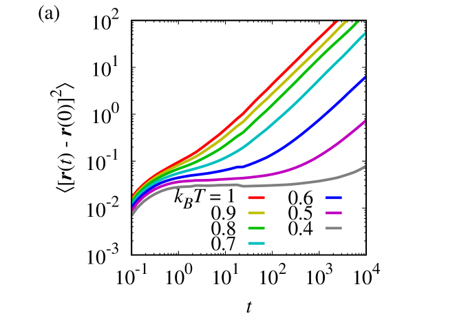
Figure 1:

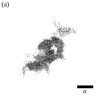
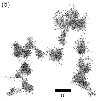
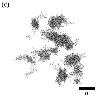
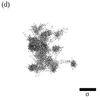
Figure 2:

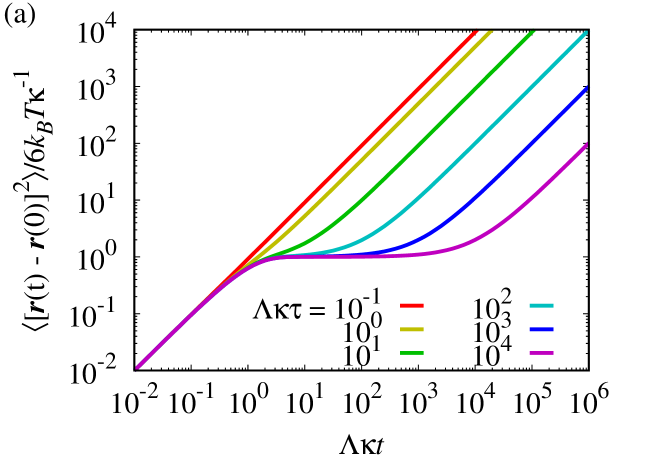
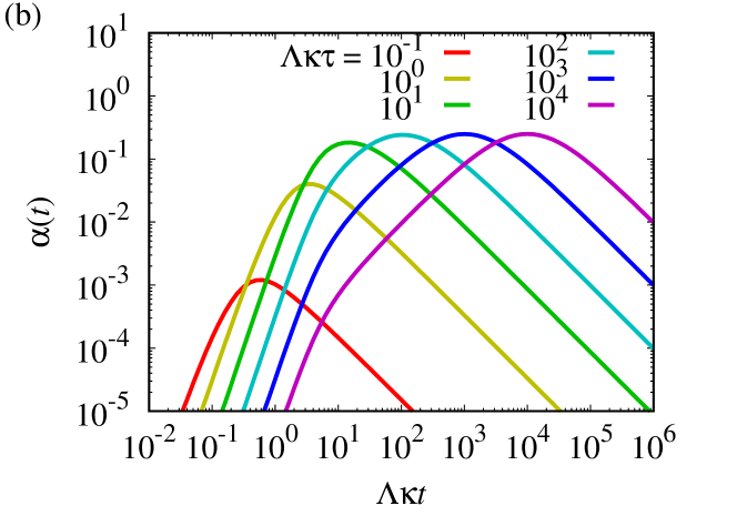
Figure 3:

References

- Müller-Plathe (2002) F. Müller-Plathe, ChemPhysChem 3, 754 (2002).
- Padding and Briels (2011) J. T. Padding and W. J. Briels, J. Phys.: Cond. Matt. 23, 233101 (2011).
- Doi and Edwards (1986) M. Doi and S. F. Edwards, The Theory of Polymer Dynamics (Oxford University Press, Oxford, 1986).
- Itami and Sasa (2017) M. Itami and S. Sasa, J. Stat. Phys. 167, 46 (2017).
- Kawasaki (1973) K. Kawasaki, J. Phys. A: Math. Nucl. Gen. 6, 1289 (1973).
- Evans and Morris (2008) D. J. Evans and G. P. Morris, Statistical Mechanics of Nonequilibrium Liquids, 2nd ed. (Cambridge University Press, Cambridge, 2008).
- Grmela and Öttinger (1997) M. Grmela and H. C. Öttinger, Phys. Rev. E 56, 6620 (1997).
- Öttinger and Grmela (1997) H. C. Öttinger and M. Grmela, Phys. Rev. E 56, 6633 (1997).
- Español (2004) P. Español, Lect. Notes Phys. 640, 69 (2004).
- Español and Warren (1995) P. Español and P. Warren, Europhys. Lett. 30, 191 (1995).
- Kinjo and Hyodo (2007) T. Kinjo and S.-a. Hyodo, Phys. Rev. E 75, 051109 (2007).
- Español (2009) P. Español, Europhys. Lett. 88, 40008 (2009).
- Kindt and Briels (2007) P. Kindt and W. J. Briels, J. Chem. Phys. 127, 134901 (2007).
- Briels (2009) W. J. Briels, Soft Matter 5, 4401 (2009).
- Briels (2015) W. Briels, “Responsive particle dynamics for modeling solvents on the mesoscopic scale,” (Forschungszentrum Jülich GmbH, 2015) pp. 557–574, in Computational Trends in Solvation and Transport in Liquids Lecture Notes, G. Sutmann and J. Grotendorst, G. Gompper and D. Marx eds.
- Chappa et al. (2012) V. C. Chappa, D. C. Morse, A. Zippelius, and M. Müller, Phys. Rev. Lett. 109, 148302 (2012).
- Uneyama and Masubuchi (2012) T. Uneyama and Y. Masubuchi, J. Chem. Phys. 137, 154902 (2012).
- Uneyama (2019) T. Uneyama, J. Chem. Phys. 150, 024901 (2019).
- (19) R. Dengler, arXiv:1506.02650.
- Gardiner (2004) C. W. Gardiner, Handbook of Stochastic Methods, 3rd ed. (Springer, Berlin, 2004).
- Kleinert (2004) H. Kleinert, Path Integrals in Quantum Mechanics, Statistics, Polymer Physics, and Finantial Markets, 3rd ed. (World Scientific, Singapore, 2004).
- Onsager and Machlup (1953) L. Onsager and S. Machlup, Phys. Rev. 91, 1505 (1953).
- Machlup and Onsager (1953) S. Machlup and L. Onsager, Phys. Rev. 91, 1512 (1953).
- Martin et al. (1973) P. C. Martin, E. D. Siggia, and H. A. Rose, Phys. Rev. A 8, 423 (1973).
- Onuki (2002) A. Onuki, Phase Transition Dynamics (Cambridge University Press, Cambridge, 2002).
- Müller and Schmid (2005) M. Müller and F. Schmid, Adv. Polym. Sci. 185, 1 (2005).
- Kawakatsu (2004) T. Kawakatsu, Statistical Physics of Polymers: An Introduction (Springer Verlag, Berlin, 2004).
- Schiff (1968) L. I. Schiff, Quantum Mechanics, 3rd ed. (McGraw-Hill, New York, 1968).
- Kullback and Leibler (1951) S. Kullback and R. A. Leibler, Annals Math. Stat. 22, 79 (1951).
- Shell (2008) M. S. Shell, J. Chem. Phys. 129, 144108 (2008).
- Español and Zúñiga (2011) P. Español and I. Zúñiga, Phys. Chem. Chem. Phys. 13, 10538 (2011).
- Hachiya et al. (2019) Y. Hachiya, T. Uneyama, T. Kaneko, and T. Akimoto, J. Chem. Phys. 151, 034502 (2019).
- Kob and Andersen (1994) W. Kob and H. C. Andersen, Phys. Rev. Lett. 73, 1376 (1994).
- Kob and Andersen (1995a) W. Kob and H. C. Andersen, Phys. Rev. E 51, 4626 (1995a).
- Kob and Andersen (1995b) W. Kob and H. C. Andersen, Phys. Rev. E 52, 4134 (1995b).
- Yamamoto and Onuki (1998a) R. Yamamoto and A. Onuki, Phys. Rev. Lett. 81, 4915 (1998a).
- Yamamoto and Onuki (1998b) R. Yamamoto and A. Onuki, Phys. Rev. E 58, 3515 (1998b).
- Kob (1999) W. Kob, J. Phys.: Cond. Matt. 11, R85 (1999).
- Vorselaars et al. (2007) B. Vorselaars, A. V. Lyulin, K. Karatasos, and M. A. J. Michels, Phys. Rev. E 75, 011504 (2007).
- Hunter and Weeks (2012) G. L. Hunter and E. R. Weeks, Rep. Prog. Phys. 75, 066501 (2012).
- Klix et al. (2015) C. L. Klix, G. Maret, and P. Keim, Phys. Rev. X 5, 041033 (2015).
- Rahman (1964) A. Rahman, Phys. Rev. 136, A405 (1964).
- Uneyama et al. (2015) T. Uneyama, T. Miyaguchi, and T. Akimoto, Phys. Rev. E 92, 032140 (2015).
- Miyaguchi et al. (2016) T. Miyaguchi, T. Akimoto, and E. Yamamoto, Phys. Rev. E 94, 012109 (2016).
- Miyaguchi (2017) T. Miyaguchi, Phys. Rev. E 96, 042501 (2017).
- Uneyama et al. (2019) T. Uneyama, T. Miyaguchi, and T. Akimoto, Phys. Rev. E 99, 032127 (2019).
- Miyaguchi et al. (2019) T. Miyaguchi, T. Uneyama, and T. Akimoto, Phys. Rev. E 100, 012116 (2019).
- Fox (1977) R. F. Fox, J. Math. Phys. 18, 2331 (1977).
- Evans and Holian (1985) D. J. Evans and B. L. Holian, J. Chem. Phys. 83, 4069 (1985).
- Leimkuhler et al. (2009) B. Leimkuhler, E. Noorizadeh, and F. Theil, J. Stat. Phys. 135, 261 (2009).
- (51) T. Nakamura, arXiv:1803.09034.
- (52) T. Uneyama, to appear in Nihon Reoroji Gakkaishi (J. Soc. Rheol. Jpn.), arXiv:1912.08481.
- Plimpton (1995) S. Plimpton, J. Comp. Phys. 117, 1 (1995).
- (54) LAMMPS Website, http://lammps.sandia.gov.
- Godrèche and Luck (2001) C. Godrèche and J. M. Luck, J. Stat. Phys. 104, 489 (2001).
- van Kampen (2007) N. G. van Kampen, Stochastic Processes in Physics and Chemistry, 3rd ed. (Elsevier, Amsterdam, 2007).