Improved guarantees and a multiple-descent curve for
Column Subset Selection and the Nyström method

Abstract

The Column Subset Selection Problem (CSSP) and the Nyström method are among the leading tools for constructing small low-rank approximations of large datasets in machine learning and scientific computing. A fundamental question in this area is: how well can a data subset of size $k$ compete with the best rank $k$ approximation? We develop techniques which exploit spectral properties of the data matrix to obtain improved approximation guarantees which go beyond the standard worst-case analysis. Our approach leads to significantly better bounds for datasets with known rates of singular value decay, e.g., polynomial or exponential decay. Our analysis also reveals an intriguing phenomenon: the approximation factor as a function of $k$ may exhibit multiple peaks and valleys, which we call a multiple-descent curve. A lower bound we establish shows that this behavior is not an artifact of our analysis, but rather it is an inherent property of the CSSP and Nyström tasks. Finally, using the example of a radial basis function (RBF) kernel, we show that both our improved bounds and the multiple-descent curve can be observed on real datasets simply by varying the RBF parameter.

1 Introduction

We consider the task of selecting a small but representative sample of column vectors from a large matrix. Known as the Column Subset Selection Problem (CSSP), this is a well-studied combinatorial optimization task with many applications in machine learning (e.g., feature selection, see Guyon & Elisseeff, 2003; Boutsidis et al., 2008), scientific computing (e.g., Chan & Hansen, 1992; Drineas et al., 2008) and signal processing (e.g., Balzano et al., 2010). In a commonly studied variant of this task, we aim to minimize the squared error of projecting all columns of the matrix onto the subspace spanned by the chosen column subset.

Definition 1 (CSSP).

Given an $m\times n$ matrix $\mathbf{A}$, pick a set $S\subseteq\{1,...,n\}$ of $k$ column indices, to minimize

$$\mathrm{Er}_{\mathbf{A}}(S):=\|\mathbf{A}-\mathbf{P}_{S}\mathbf{A}\|_{F}^{2},$$

where $\|\cdot\|_{F}$ is the Frobenius norm, $\mathbf{P}_{S}$ is the projection onto $\mathrm{span}\{\mathbf{a}_{i}:i\in S\}$ and $\mathbf{a}_{i}$ denotes the $i$th column of $\mathbf{A}$.

Another variant of the CSSP emerges in the kernel setting under the name Nyström method (Williams & Seeger, 2001; Drineas & Mahoney, 2005; Gittens & Mahoney, 2016). We also discuss this variant, showing how our analysis applies in this context. Both the CSSP and the Nyström method are ways of constructing accurate low-rank approximations by using submatrices of the target matrix. Therefore, it is natural to ask how close we can get to the best possible rank $k$ approximation error:

$${\textsc{OPT}_{k}}:=\!\!\min_{\mathbf{B}:\,\mathrm{rank}(\mathbf{B})=k}\!\!\|\mathbf{A}-\mathbf{B}\|_{F}^{2}\leq\min_{S:\,|S|=k}\mathrm{Er}_{\mathbf{A}}(S).$$

Our goal is to find a subset $S$ of size $k$ for which the ratio between $\mathrm{Er}_{\mathbf{A}}(S)$ and ${\textsc{OPT}_{k}}$ is small. Furthermore, a brute force search requires iterating over all ${n\choose k}$ subsets, which is prohibitively expensive, so we would like to find our subset more efficiently.

Figure 1: Empirical study of the expected approximation factor $\mathbb{E}[\mathrm{Er}_{\mathbf{A}}(S)]/{\textsc{OPT}_{k}}$ for a $k$-DPP with different subset sizes $|S|=k$, compared to our theory. We use a data matrix $\mathbf{A}$ whose spectrum exhibits two sharp drops, demonstrating multiple-descent. The lower bounds are based on Theorem 3, whereas, as our upper bound, we plot the minimum over all $\Phi_{s}(k)$ from Theorem 1. Note that multiple-descent vanishes under smooth spectral decay, resulting in improved guarantees (see Theorem 2 and Figure 2).

Extensive literature has been dedicated to developing algorithms for the CSSP (an in depth discussion of the related work can be found in Appendix A). In terms of worst-case analysis, Deshpande et al. (2006) gave a randomized method which returns a set $S$ of size $k$ such that:

$$\frac{\mathbb{E}[\mathrm{Er}_{\mathbf{A}}(S)]}{{\textsc{OPT}_{k}}}\leq k+1.$$ (1)

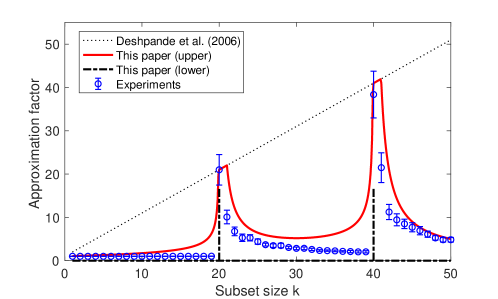
While the original algorithm was slow, efficient implementations have been provided since then (e.g., see Deshpande & Rademacher, 2010; Dereziński, 2019). The method belongs to the family of cardinality constrained Determinantal Point Processes (DPPs, see Dereziński & Mahoney, 2020), and will be denoted as $S\sim k\text{-}{\mathrm{DPP}}(\mathbf{A}^{\scriptscriptstyle{\top}}\mathbf{A})$. The approximation factor $k+1$ is optimal in the worst-case, since for any $0<k<n\leq m$ and $0<\delta<1$, an $m\times n$ matrix $\mathbf{A}$ can be constructed for which $\frac{\mathrm{Er}_{\mathbf{A}}(S)}{{\textsc{OPT}_{k}}}\geq(1-\delta)(k+1)$ for all subsets $S$ of size $k$. Yet it is known that, in practice, CSSP algorithms perform better than worst-case, so the question we consider is: how can we go beyond the usual worst-case analysis to accurately reflect what is possible in the CSSP?

Contributions. We provide improved guarantees for the CSSP approximation factor, which go beyond the worst-case analysis and which lead to surprising conclusions.

1. New upper bounds: We develop a family of upper bounds on the CSSP approximation factor (Theorem 1), which we call the Master Theorem as they can be used to derive a number of new guarantees. In particular, we show that when the data matrix $\mathbf{A}$ exhibits a known spectral decay, then (1) can often be drastically improved (Theorem 2).

2. New lower bound: Even though the worst-case upper bound in (1) can often be loose, there are cases when it cannot be improved. We give a new lower bound construction (Theorem 3) showing that there are matrices $\mathbf{A}$ for which multiple different subset sizes exhibit worst-case behavior.

3. Multiple-descent curve: Our upper and lower bounds reveal that for some matrices the CSSP approximation factor can exhibit peaks and valleys as a function of the subset size $k$ (see Figure 1). We show that this phenomenon is an inherent property of the CSSP (Corollary 1).

1.1 Main results

Our upper bounds rely on the notion of effective dimensionality called stable rank (Alaoui & Mahoney, 2015). Here, we use an extended version of this concept, as defined by Bartlett et al. (2019).

Definition 2 (Stable rank).

Let $\lambda_{1}\geq\lambda_{2}\geq...$ denote the eigenvalues of the matrix $\mathbf{A}^{\scriptscriptstyle{\top}}\mathbf{A}$. For $0\leq s<\mathrm{rank}(\mathbf{A})$, we define the stable rank of order $s$ as ${\mathrm{sr}}_{s}(\mathbf{A})=\lambda_{s+1}^{-1}\sum_{i>s}\lambda_{i}$.

In the following result, we define a family of functions $\Phi_{s}(k)$ which bound the approximation factor $\mathrm{Er}_{\mathbf{A}}(S)/{\textsc{OPT}_{k}}$ in the range of $k$ between $s$ and $s+{\mathrm{sr}}_{s}(\mathbf{A})$. We call this the Master Theorem because we use it to derive a number of more specific upper bounds.

Theorem 1 (Master Theorem).

Given $0\leq s<\mathrm{rank}(\mathbf{A})$, let $t_{s}=s+{\mathrm{sr}}_{s}(\mathbf{A})$, and suppose that $s+\frac{7}{\epsilon^{4}}\ln^{2}\!\frac{1}{\epsilon}\leq k\leq t_{s}-1$, where $0<\epsilon\leq\frac{1}{2}$. If $S\sim k$-${\mathrm{DPP}}(\mathbf{A}^{\scriptscriptstyle{\top}}\mathbf{A})$, then

$$\frac{\mathbb{E}[\mathrm{Er}_{\mathbf{A}}(S)]}{{\textsc{OPT}_{k}}}\leq(1+2\epsilon)^{2}\,\Phi_{s}(k),\qquad\text{where}\quad\Phi_{s}(k)=\big{(}1+\tfrac{s}{k-s}\big{)}\sqrt{1+\tfrac{2(k-s)}{t_{s}-k}\,}.$$

Note that we separated out the dependence on $\epsilon$ from the function $\Phi_{s}(k)$, because the term $(1+2\epsilon)^{2}$ is an artifact of a concentration of measure analysis that is unlikely to be of practical significance. In fact, we believe that the dependence on $\epsilon$ can be eliminated from the statement entirely (see Conjecture 1).

We next examine the consequences of the Master Theorem, starting with a sharp transition that occurs as $k$ approaches the stable rank of $\mathbf{A}$.

Remark 1 (Sharp transition).

For any $k$ it is true that:

1. For all $\mathbf{A}$, if $k\leq{\mathrm{sr}}_{0}(\mathbf{A})\!-\!1$, then there is a subset $S$ of size $k$ such that $\frac{\mathrm{Er}_{\mathbf{A}}(S)}{{\textsc{OPT}_{k}}}=O(\sqrt{k}\,)$.

2. There is $\mathbf{A}$ such that ${\mathrm{sr}}_{0}(\mathbf{A})\!-\!1<k<{\mathrm{sr}}_{0}(\mathbf{A})$ and for every size $k$ subset $S$, $\frac{\mathrm{Er}_{\mathbf{A}}(S)}{{\textsc{OPT}_{k}}}\geq 0.9\,k$.

Part 1 of the remark follows from the Master Theorem by setting $s=0$, whereas part 2 follows from the lower bound of Guruswami & Sinop (2012). Observe how the worst-case approximation factor jumps from $O(\sqrt{k}\,)$ to $\Omega(k)$, as $k$ approaches ${\mathrm{sr}}_{0}(\mathbf{A})$. An example of this sharp transition is shown in Figure 1, where the stable rank of $\mathbf{A}$ is around $20$.

While certain matrices directly exhibit the sharp transition from Remark 1, many do not. In particular, for matrices with a known rate of spectral decay, the Master Theorem can be used to provide improved guarantees on the CSSP approximation factor over all subset sizes.

To illustrate this, we give novel bounds for the two most commonly studied decay rates: polynomial and exponential.

Theorem 2 (Examples without sharp transition).

Let $\lambda_{1}\!\geq\!\lambda_{2}\!\geq\!...$ be the eigenvalues of $\mathbf{A}^{\scriptscriptstyle{\top}}\mathbf{A}$. There is an absolute constant $c$ such that for any $0\!<\!c_{1}\!\leq\!c_{2}$, with $\gamma=c_{2}/c_{1}$, if:
1. (polynomial spectral decay) $c_{1}i^{-p}\!\leq\!\lambda_{i}\!\leq\!c_{2}i^{-p}$ $\forall_{i}$, with $p>1$, then $S\sim k$-${\mathrm{DPP}}(\mathbf{A}^{\scriptscriptstyle{\top}}\mathbf{A})$ satisfies

$$\frac{\mathbb{E}[\mathrm{Er}_{\mathbf{A}}(S)]}{{\textsc{OPT}_{k}}}\leq c\gamma p.$$

2. (exponential spectral decay) $c_{1}(1\!-\!\delta)^{i}\leq\lambda_{i}\leq c_{2}(1\!-\!\delta)^{i}$ $\forall_{i}$, $\delta\in(0,1)$, then $S\sim k$-${\mathrm{DPP}}(\mathbf{A}^{\scriptscriptstyle{\top}}\mathbf{A})$ satisfies

$$\frac{\mathbb{E}[\mathrm{Er}_{\mathbf{A}}(S)]}{{\textsc{OPT}_{k}}}\leq c\gamma(1+\delta k).$$

Note that for polynomial decay, unlike in (1), the approximation factor is constant, i.e., it does not depend on $k$. For exponential decay, our bound provides an improvement over (1) when $\delta=o(1)$. To illustrate how these types of bounds can be obtained from the Master Theorem, consider the function $\Phi_{s}(k)$ for some $s>0$. The first term in the function, $1+\frac{s}{k-s}$, decreases with $k$, whereas the second term (the square root) increases, albeit at a slower rate. This creates a U-shaped curve which, if sufficiently wide, has a valley where the approximation factor can get arbitrarily close to 1. This will occur when ${\mathrm{sr}}_{s}(\mathbf{A})$ is large, i.e., when the spectrum of $\mathbf{A}^{\scriptscriptstyle{\top}}\mathbf{A}$ has a relatively flat region after the $s$th eigenvalue (Figure 1 for $k$ between 20 and 40). Note that a peak value of some function $\Phi_{s_{1}}$ may coincide with a valley of some $\Phi_{s_{2}}$, so only taking a minimum over all functions reveals the true approximation landscape predicted by the Master Theorem. To prove Theorem 2, we show that the stable ranks ${\mathrm{sr}}_{s}(\mathbf{A})$ are sufficiently large so that any $k$ lies in the valley of some function $\Phi_{s}(k)$ (see Section 2).

The peaks and valleys of the CSSP approximation factor suggested by Theorem 1 are in fact an inherent property of the problem, rather than an artifact of our analysis or the result of using a particular algorithm. We prove this by constructing a family of matrices $\mathbf{A}$ for which the best possible approximation factor is large, i.e., close to the worst-case upper bound of Deshpande et al. (2006), not just for one size $k$, but for a sequence of increasing sizes.

Theorem 3 (Lower bound).

For any $\delta\in(0,1)$ and $0\!=\!k_{0}\!<\!k_{1}\!<\!...\!<\!k_{t}\!<\!n\leq m$, there is a matrix $\mathbf{A}\in\mathbb{R}^{m\times n}$ such that for any subset $S$ of size $k_{i}$, where $i\in\{1,...,t\}$,

$$\frac{\mathrm{Er}_{\mathbf{A}}(S)}{\textsc{OPT}_{k_{i}}}\geq(1-\delta)(k_{i}-k_{i-1}).$$

Combining the Master Theorem with the lower bound of Theorem 3 we can easily provide an example matrix for which the optimal solution to the CSSP problem exhibits multiple peaks and valleys. We refer to this phenomenon as the multiple-descent curve.

Corollary 1 (Multiple-descent curve).

For $t\in\mathbb{N}$ and $\delta\in(0,1)$, there is a sequence $0<k_{1}^{l}<k_{1}^{u}<k_{2}^{l}<k_{2}^{u}<...<k_{t}^{l}<k_{t}^{u}$ and $\mathbf{A}\in\mathbb{R}^{m\times n}$ such that for any $i\in\{1,...,t\}$:

$$\min_{S:|S|=k_{i}^{l}}\frac{\mathrm{Er}_{\mathbf{A}}(S)}{\textsc{OPT}_{k_{i}^{l}}}\leq 1+\delta\qquad\text{and }\qquad\min_{S:|S|=k_{i}^{u}}\frac{\mathrm{Er}_{\mathbf{A}}(S)}{\textsc{OPT}_{k_{i}^{u}}}\geq(1-\delta)(k_{i}^{u}+1).$$

Connection to double descent.

A number of phase transitions have been recently observed in the machine learning literature which are commonly dubbed double descent. The term was introduced by Belkin et al. (2019a) in the context of generalization error of statistical learning, however Poggio et al. (2019) observed that the behavior of the generalization error, at least for linear models, can be explained by a more fundamental double descent phenomenon observed in the condition number of random matrices. Also, Liao et al. (2020) showed that double descent is merely a manifestation of the spectral phase transitions in high-dimensional random kernel matrices. Further, Liang et al. (2020) observed that the spectral phase transitions of certain kernels can lead to multiple double descent peaks. The multiple-descent phenomenon in the CSSP that emerges from our analysis is related to those works in that the spectral properties of the data matrix (and, in particular, the condition number) determine the peaks (i.e., phase transitions) discussed in Corollary 1. Those parallels manifest themselves most clearly when comparing our analysis to the work of Bartlett et al. (2019), which uses the same notion of stable rank as we do, and Dereziński et al. (2019b), where determinantal sampling plays a central role in the analysis of double descent. However, we stress that there are also important differences in our setting: (1) the CSSP is a deterministic optimization task, and (2) we study the approximation factor, rather than the generalization error (further discussion in Appendix A).

1.2 The Nyström method

We briefly discuss how our results translate to guarantees for the Nyström mehod, a variant of the CSSP in the kernel setting which has gained considerable interest in the machine learning literature (Drineas & Mahoney, 2005; Gittens & Mahoney, 2016). In this context, rather than being given the column vectors explicitly, we consider the $n\times n$ matrix $\mathbf{K}$ whose entry $(i,j)$ is the dot product between the $i$th and $j$th vector in the kernel space, $\langle\mathbf{a}_{i},\mathbf{a}_{j}\rangle_{\text{K}}$. A Nyström approximation of $\mathbf{K}$ based on subset $S$ is defined as ${\widehat{\mathbf{K}}}(S)=\mathbf{C}\mathbf{B}^{\dagger}\mathbf{C}^{\scriptscriptstyle{\top}}$, where $\mathbf{B}$ is the $|S|\times|S|$ submatrix of $\mathbf{K}$ indexed by $S$, whereas $\mathbf{C}$ is the $n\times|S|$ submatrix with columns indexed by $S$. The Nyström method has many applications in machine learning, including for kernel machines (Williams & Seeger, 2001), Gaussian Process regression (Burt et al., 2019) and Independent Component Analysis (Bach & Jordan, 2003).

Remark 2.

If $\mathbf{K}=\mathbf{A}^{\scriptscriptstyle{\top}}\mathbf{A}$ and $\|\cdot\|_{*}$ is the trace norm, then $\big{\|}\mathbf{K}-{\widehat{\mathbf{K}}}(S)\big{\|}_{*}=\mathrm{Er}_{\mathbf{A}}(S)$ for all $S\subseteq\{1,...,n\}$. Moreover, the trace norm error of the best rank $k$ approximation of $\mathbf{K}$, is equal to the squared Frobenius norm error of the best rank $k$ approximation of $\mathbf{A}$, i.e.,

$$\min_{{\widehat{\mathbf{K}}}:\,\mathrm{rank}(\mathbf{K})=k}\|\mathbf{K}-{\widehat{\mathbf{K}}}\|_{*}={\textsc{OPT}_{k}}.$$

This connection was used by Belabbas & Wolfe (2009) to adapt the $k+1$ approximation factor bound of Deshpande et al. (2006) to the Nyström method. Similarly, all of our results for the CSSP, including the multiple-descent curve that we have observed, can be translated into analogous statements for the trace norm approximation error in the Nyström method. Of particular interest are the improved bounds for kernel matrices with known eigenvalue decay rates. Such matrices arise naturally in machine learning when using standard kernel functions such as the Gaussian Radial Basis Function (RBF) kernel (a.k.a. the squared exponential kernel) and the Matérn kernel (Burt et al., 2019).

RBF kernel: If $\langle\mathbf{a}_{i},\mathbf{a}_{j}\rangle_{\text{K}}=\exp(-\|\mathbf{a}_{i}\!-\!\mathbf{a}_{j}\|^{2}/\sigma^{2})$ and the data comes from $\mathcal{N}(0,\eta^{2})$, then, for large $n$, $\lambda_{i}\!\asymp\!\lambda_{1}(\frac{b}{a+b+c})^{i}$, where $a=\frac{1}{4\eta^{2}}$, $b=\frac{1}{\sigma^{2}}$ and $c=\sqrt{a^{2}\!+\!2ab}$ (Santa et al., 1997), so Theorem 2 yields an approximation factor of $O(1\!+\!\frac{a+c}{a+b+c}k)$, better than $k\!+\!1$ when $\sigma^{2}\ll\eta^{2}$. Note that the parameter $\sigma$ defines the size of a neighborhood around which the data points are deemed similar by the RBF kernel. Therefore, smaller $\sigma$ means that each data point has fewer similar neighbors.

Matérn kernel: If $\mathbf{K}$ is the Matérn kernel with parameters $\nu$ and $\ell$ and the data is distributed according to a uniform measure in one dimension, then $\lambda_{i}\asymp\lambda_{1}i^{-2\nu-1}$ (Rasmussen & Williams, 2006), so Theorem 2 yields a Nyström approximation factor of $O(1+\nu)$ for any subset size $k$.

In Section 4, we also empirically demonstrate our improved guarantees and the multiple-descent curve for the Nyström method with the RBF kernel.

2 Upper bounds

In this section, we derive the upper bound given in Theorem 1 by using a novel expectation formula for the squared projection error of a DPP. We then show how this result can be used to obtain improved guarantees for matrices with known eigenvalue decays, i.e., Theorem 2. Our analysis heavily relies on the theory of DPPs (Dereziński & Mahoney, 2020), so for completeness, in Appendix B we provide a brief summary of DPPs and the relevant results.

Let $S\sim{\mathrm{DPP}}(\frac{1}{\alpha}\mathbf{A}^{\scriptscriptstyle{\top}}\mathbf{A})$ denote a distribution over all subsets $S\subseteq[n]$ so that $\mathrm{Pr}(S)\propto\det(\frac{1}{\alpha}\mathbf{A}_{S}^{\scriptscriptstyle{\top}}\mathbf{A}_{S})$, where $\alpha>0$. Then, $k$-${\mathrm{DPP}}(\mathbf{A}^{\scriptscriptstyle{\top}}\mathbf{A})$ is simply a restriction of ${\mathrm{DPP}}(\frac{1}{\alpha}\mathbf{A}^{\scriptscriptstyle{\top}}\mathbf{A})$ to the subsets of size $k$ (regardless of the choice of $\alpha$). However, the expected subset size for ${\mathrm{DPP}}(\frac{1}{\alpha}\mathbf{A}^{\scriptscriptstyle{\top}}\mathbf{A})$ does depend on $\alpha$. Our analysis relies on a careful selection of this parameter. In Lemma 6 (Appendix B), we show the following expectation formula for the CSSP approximation error:

$$\mathbb{E}[\mathrm{Er}_{\mathbf{A}}(S)]=\mathbb{E}[|S|]\cdot\alpha,\quad\text{for}\quad S\sim{\mathrm{DPP}}(\tfrac{1}{\alpha}\mathbf{A}^{\scriptscriptstyle{\top}}\mathbf{A}).$$

If we set $\alpha={\textsc{OPT}_{k}}=\sum_{i=k+1}^{n}\lambda_{i}$, where $\lambda_{i}$ are the eigenvalues of $\mathbf{A}^{\scriptscriptstyle{\top}}\mathbf{A}$ in decreasing order, then:

$$\mathbb{E}[|S|] =\sum_{i=1}^{n}\frac{\lambda_{i}}{\alpha+\lambda_{i}}\leq\sum_{i=1}^{k}\frac{\lambda_{i}}{\alpha+\lambda_{i}}+1\leq k+1.$$

This recovers the upper bound of Deshpande et al. (2006), i.e., $\mathbb{E}[\mathrm{Er}_{\mathbf{A}}(S)]\leq(k+1){\textsc{OPT}_{k}}$, except that the subset size is randomized with expectation bounded by $k+1$, instead of a fixed subset size equal $k$. However, a more refined choice of the parameter $\alpha$ allows us to significantly improve on the above error bound in certain regimes, as shown below.

Lemma 1.

For any $\mathbf{A}$, $0\leq\epsilon<1$ and $s<k<t_{s}$, where $t_{s}=s+{\mathrm{sr}}_{s}(\mathbf{A})$, say $S\sim{\mathrm{DPP}}(\frac{1}{\alpha}\mathbf{A}^{\scriptscriptstyle{\top}}\mathbf{A})$ for $\alpha=\frac{\gamma_{s}(k){\textsc{OPT}_{k}}}{(1-\epsilon)(k-s)}$ and $\gamma_{s}(k):=\sqrt{1+\frac{2(k-s)}{t_{s}-k}\,}$. Then, defining $\Phi_{s}(k):=\big{(}1+\frac{s}{k-s}\big{)}\,\gamma_{s}(k)$,

$$\frac{\mathbb{E}\big{[}\mathrm{Er}_{\mathbf{A}}(S)\big{]}}{{\textsc{OPT}_{k}}}\leq\frac{\Phi_{s}(k)}{1-\epsilon}\quad\text{and}\quad\mathbb{E}[|S|]\leq k-\epsilon\,\frac{k-s}{\gamma_{s}(k)}.$$

Note that, setting $\epsilon=0$, the above lemma implies that we can achieve approximation factor $\Phi_{s}(k)$ with a DPP whose expected size is bounded by $k$. We introduce $\epsilon$ so that we can convert the bound from DPP to the fixed size k-DPP via a concentration argument. Intuitively, our strategy is to show that the randomized subset size of a DPP is sufficiently concentrated around its expectation that with high probability it will be bounded by $k$, and for this we need the expectation to be strictly below $k$. A careful application of the Chernoff bound for a Poisson binomial random variable yields the following concentration bound.

Lemma 2.

Let $S$ be as in Lemma 1 with $\epsilon\leq\frac{1}{2}$. If $s+\frac{7}{\epsilon^{4}}\ln^{2}\!\frac{1}{\epsilon}\leq k\leq t_{s}-1$, then $\mathrm{Pr}(|S|>k)\leq\epsilon$.

Finally, any expected bound for random size DPPs can be converted to an expected bound for a fixed size k-DPP via the following result.

Lemma 3.

For any $\mathbf{A}\in\mathbb{R}^{m\times n}$, $k\in[n]$ and $\alpha>0$, if $S\sim{\mathrm{DPP}}(\frac{1}{\alpha}\mathbf{A}^{\scriptscriptstyle{\top}}\mathbf{A})$ and $S^{\prime}\sim k$-${\mathrm{DPP}}(\mathbf{A}^{\scriptscriptstyle{\top}}\mathbf{A})$, then

$$\mathbb{E}\big{[}\mathrm{Er}_{\mathbf{A}}(S^{\prime})\big{]}\leq\mathbb{E}\big{[}\mathrm{Er}_{\mathbf{A}}(S)\mid|S|\leq k\big{]}.$$

The above inequality may seem intuitively obvious since adding more columns to a set $S$ to complete it to size $k$ always reduces the error. However, a priori, it could happen that going from subsets of size $k-1$ to subsets of size $k$ results in a redistribution of probabilities to the subsets with larger error. To show that this will not happen, our proof relies on classic but non-trivial combinatorial bounds called Newton’s inequalities. Putting together Lemmas 1, 2 and 3, we obtain our Master Theorem.

Proof of Theorem 1  Let $S\sim{\mathrm{DPP}}(\frac{1}{\alpha}\mathbf{A}^{\scriptscriptstyle{\top}}\mathbf{A})$ be sampled as in Lemma 1, and let $S^{\prime}\sim k$-${\mathrm{DPP}}(\mathbf{A}^{\scriptscriptstyle{\top}}\mathbf{A})$. We have:

$$\mathbb{E}\big{[}\mathrm{Er}_{\mathbf{A}}(S^{\prime})\big{]}\overset{(a)}{\leq}\mathbb{E}\big{[}\mathrm{Er}_{\mathbf{A}}(S)\mid|S|\leq k\big{]}\leq\frac{\mathbb{E}\big{[}\mathrm{Er}_{\mathbf{A}}(S)\big{]}}{\mathrm{Pr}(|S|\leq k)}\overset{(b)}{\leq}\frac{\Phi_{s}(k)}{(1-\epsilon)^{2}}\cdot{\textsc{OPT}_{k}},$$

where $(a)$ follows from Lemma 3 and $(b)$ follows from Lemmas 1 and 2. Since $0<\epsilon\leq\frac{1}{2}$, we have $\frac{1}{(1-\epsilon)^{2}}\leq(1+2\epsilon)^{2}$, which completes the proof.  

Figure 2: Illustration of the upper bound functions $\Phi_{s}(k)$ for different values of $s$, with a $200\times 200$ matrix $\mathbf{A}$ such that the $i$th eigenvalue of $\mathbf{A}^{\scriptscriptstyle{\top}}\mathbf{A}$ is set to: (top) $1/i$; (bottom) $1$ for $i<30$ and $0.01$ for $i\geq 30$. For each function, we marked the window of applicable $k$’s with a horizontal line. For polynomial spectral decay (top), the stable rank ${\mathrm{sr}}_{s}(\mathbf{A})$ (i.e., the width of the window starting at $s$) increases, while for the sharp spectrum drop (bottom) the stable rank shrinks as the window approaches the drop, causing a peak in the upper bound.

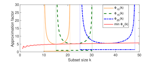
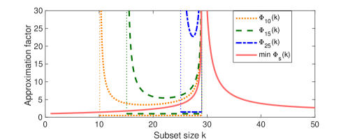
We now demonstrate how Theorem 1 can be used as the Master Theorem to derive new bounds on the CSSP approximation factor under additional assumptions on the singular value decay of matrix $\mathbf{A}$. Rather than a single upper bound, Theorem 1 provides a family of upper bounds $\Phi_{s}$, each with a range of applicable values $k$. Since each $\Phi_{s}(k)$ forms a U-shaped curve, its smallest point falls near the middle of that range. In Figure 2 we visualize these bounds as a sliding window that sweeps across the axis representing possible subset sizes. The width of the window varies: when it starts at $s$ then its width is the stable rank ${\mathrm{sr}}_{s}(\mathbf{A})$. The wider the window, the lower is the valley of the corresponding U-curve. Thus, when bounding the approximation factor for a given $k$, we should choose the widest window such that $k$ falls near the bottom of its U-curve. Showing a guarantee that holds for all $k$ requires lower-bounding the stable ranks ${\mathrm{sr}}_{s}(\mathbf{A})$ for each $s$. This is straightforward for both polynomial and exponential decay. Specifically, using the notation from Theorem 2, in Appendix E we prove that:

$${\mathrm{sr}}_{s}(\mathbf{A})=\begin{cases}\Omega(s/p),&\text{for polynomial rate $\lambda_{i}\asymp 1/i^{p}$},\\ \Omega(1/\delta),&\text{for exponential rate $\lambda_{i}\asymp(1-\delta)^{i}$}.\end{cases}$$

As an example, Figure 2 (left) shows that the stable rank ${\mathrm{sr}}_{s}(\mathbf{A})$, i.e., the width of the window starting at $s$, grows linearly with $s$ for eigenvalues decaying polynomially with $p=1$. As a result, the bottom of each U-shaped curve remains at roughly the same level, making the CSSP approximation factor independent of $k$, as in Theorem 2. In contrast, Figure 2 (right) provides the same plot for a different matrix $\mathbf{A}$ with a sharp drop in the spectrum. The U-shaped curves cannot slide smoothly across that drop because of the shrinking stable ranks, which results in a peak similar to the ones observed in Figure 1.

3 Lower bound

As discussed in the previous section, our upper bounds for the CSSP approximation factor exhibit a peak (a high point, with the bound decreasing on either side) around a subset size $k$ when there is a sharp drop in the spectrum of $\mathbf{A}$ around the $k$th singular value. It is natural to ask whether this peak is an artifact of our analysis, or a property of the k-DPP distribution, or whether even optimal CSSP subsets exhibit this phenomenon. In this section, we extend a lower bound construction of Deshpande et al. (2006) and use it to show that for certain matrices the approximation factor of the optimal CSSP subset, i.e., $\min_{|S|=k}\mathrm{Er}_{\mathbf{A}}(S)/{\textsc{OPT}_{k}}$, can exhibit not just one but any number of peaks as a function of $k$, showing that the multiple-descent curve in Figure 1 describes a real phenomenon in the CSSP.

The lower bound construction of Deshpande et al. (2006) relies on arranging the column vectors of a $(k+1)\times(k+1)$ matrix $\mathbf{A}$ into a centered symmetric $k$-dimensional simplex. This way, the $k+1$ columns are spanning a $k$ dimensional subspace which contains the $k$ leading singular vectors of $\mathbf{A}$. They then proceed to shift the columns slightly in the direction orthogonal to that subspace so that the $(k+1)$st singular value of $\mathbf{A}$ becomes non-zero. This results in an instance of the CSSP with a sharp drop in the spectrum. Due to the symmetry in this construction, all subsets of size $k$ have an identical squared projection error. It is easy to show that this error satisfies $\mathrm{Er}_{\mathbf{A}}(S)\geq(1-\delta)(k+1){\textsc{OPT}_{k}}$, where $\delta$ is a parameter which depends on the condition number of matrix $\mathbf{A}$ and it can be driven arbitrarily close to $0$. Another variant of this construction was also provided by Guruswami & Sinop (2012). The key limitation of both of these constructions is that they only provide a lower bound for a single subset size $k$ in a given matrix, whereas our goal is to show that the CSSP can exhibit the multiple-descent curve, which requires lower bounds for multiple different values of $k$ holding with respect to the same matrix $\mathbf{A}$.

Our strategy for constructing the lower bound matrix is to concatenate together multiple sets of columns, each of which represents a simplex spanning some subspace of $\mathbb{R}^{m}$. The key challenge that we face in this approach is that, unlike in the construction of Deshpande et al. (2006), different subsets of the same size will have different projection errors.

Lemma 4.

Fix $\delta\in(0,1)$ and consider unit vectors $\mathbf{a}_{i,j}\in\mathbb{R}^{m}$ in general position, where $i\in[t]$, $j\in[l_{i}]$, such that $\sum_{j}\mathbf{a}_{i,j}=0$ for each $i$, and for any $i,j,i^{\prime},j^{\prime}$, if $i\neq i^{\prime}$ then $\mathbf{a}_{i,j}$ is orthogonal to $\mathbf{a}_{i^{\prime}\!,j^{\prime}}$. Also, let unit vectors $\{\mathbf{v}_{i}\}_{i\in[t]}$ be orthogonal to each other and to all $\mathbf{a}_{i,j}$. There are positive scalars $\alpha_{i},\beta_{i}$ for $i\in[t]$ such that matrix $\mathbf{A}$ with columns $\alpha_{i}\mathbf{a}_{i,j}+\beta_{i}\mathbf{v}_{i}$ over all $i$ and $j$ satisfies:

$$\min_{|S|=k_{i}}\frac{\mathrm{Er}_{\mathbf{A}}(S)}{\mathrm{OPT}_{k_{i}}}\geq(1-\delta)l_{i},\quad\text{for }k_{i}=l_{1}+...+l_{i}-1.$$

Proof of Theorem 3  We let $l_{1}=k_{1}+1$ and then for $i>1$ we set $l_{i}=k_{i}-k_{i-1}$. We then construct the vectors $\mathbf{a}_{i,j}$ that satisfy Lemma 4 by letting each set $\{\mathbf{a}_{i,j}\}_{j}$ be the corners of a centered $(l_{i}-1)$-dimensional regular simplex. We ensure that each simplex is orthogonal to every other simplex by placing them in orthogonal subspaces.  

4 Empirical evaluation

In this section, we provide an empirical evaluation designed to demonstrate how our improved guarantees for the CSSP and Nyström method, as well as the multiple-descent phenomenon, can be easily observed on real datasets. We use a standard experimental setup for data subset selection using the Nyström method (Gittens & Mahoney, 2016), where an $n\times n$ kernel matrix $\mathbf{K}$ for a dataset of size $n$ is defined so that the entry $(i,j)$ is computed using the Gaussian Radial Basis Function (RBF) kernel: $\langle\mathbf{a}_{i},\mathbf{a}_{j}\rangle_{\text{K}}=\exp(-\|\mathbf{a}_{i}\!-\!\mathbf{a}_{j}\|^{2}/\sigma^{2})$, where $\sigma$ is a free parameter. We are particularly interested in the effect of varying $\sigma$. Nyström subset selection is performed using $S\sim k$-${\mathrm{DPP}}(\mathbf{K})$ (Definition 3), and we plot the expected approximation factor $\mathbb{E}[\|\mathbf{K}-{\widehat{\mathbf{K}}}(S)\|_{*}]/{\textsc{OPT}_{k}}$ (averaged over 1000 runs), where ${\widehat{\mathbf{K}}}(S)$ is the Nyström approximation of $\mathbf{K}$ based on the subset $S$ (see Section 1.2), $\|\cdot\|_{*}$ is the trace norm, and ${\textsc{OPT}_{k}}$ is the trace norm error of the best rank $k$ approximation. Additional experiments, using greedy selection instead of a k-DPP, are in Appendix H. As discussed in Section 1.2, this task is equivalent to the CSSP task defined on the matrix $\mathbf{A}$ such that $\mathbf{K}=\mathbf{A}^{\scriptscriptstyle{\top}}\mathbf{A}$.

The aim of our empirical evaluation is to verify the following two claims motivated by our theory (and to illustrate that doing so is as easy as varying the RBF parameter $\sigma$):

1. When the spectral decay is sufficiently slow/smooth, the approximation factor for CSSP/Nyström is much better than suggested by previous worst-case bounds.

2. A drop in spectrum around the $k$th eigenvalue results in a peak in the approximation factor near subset size $k$. Several drops result in the multiple-descent curve.

In Figure 3 (top), we plot the approximation factor against the subset size $k$ (in the range of 1 to 40) for an artificial toy dataset and for two benchmark regression datasets from the Libsvm repository (bodyfat and eunite2001, see Chang & Lin, 2011). The toy dataset is constructed by scaling the eigenvalues of a random $50\times 50$ Gaussian matrix so that the spectrum is flat with a single drop at the $21$-st eigenvalue. For each dataset, in Figure 3 (bottom), we also show the top 40 eigenvalues of the kernel $\mathbf{K}$ in decreasing order. For the toy dataset, to maintain full control over the spectrum we use the linear kernel $\langle\mathbf{a}_{i},\mathbf{a}_{j}\rangle_{\text{K}}=\mathbf{a}_{i}^{\scriptscriptstyle{\top}}\mathbf{a}_{j}$, and we show results for three different values of the condition number $\kappa$ of kernel $\mathbf{K}$. For the benchmark datasets, we show results on the RBF kernel with three different values of the parameter $\sigma$.

Figure 3: Top three plots show the Nyström approximation factor $\mathbb{E}[\|\mathbf{K}-{\widehat{\mathbf{K}}}(S)\|_{*}]/{\textsc{OPT}_{k}}$, where $S\sim k$-${\mathrm{DPP}}(\mathbf{K})$ (experiments using greedy selection instead of a k-DPP are in Appendix H), for a toy dataset ($\kappa$ is the condition number) and two Libsvm datasets ($\sigma$ is the RBF parameter). Error bars show three times the standard error of the mean over 1000 trials. Bottom three plots show the spectral decay for the top $40$ eigenvalues of each kernel $\mathbf{K}$. Note that the peaks in the approximation factor align with the drops in the spectrum.

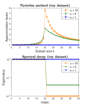
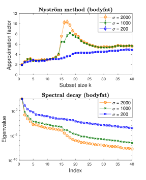
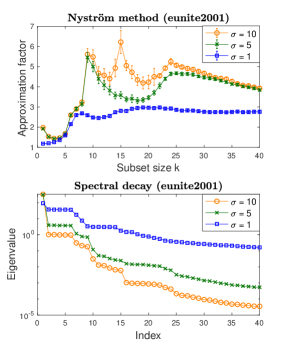
Examining the toy dataset (Figure 3, left), it is apparent that a larger drop in spectrum leads to a sharper peak in the approximation factor as a function of the subset size $k$, whereas a flat spectrum results in the approximation factor being close to $1$. A similar trend is observed for dataset bodyfat (Figure 3, center), where large parameter $\sigma$ results in a peak that is aligned with a spectrum drop, while decreasing $\sigma$ makes the spectrum flatter and the factor closer to $1$. Finally, dataset eunite2001 (Figure 3, right) exhibits a full multiple-descent curve with up to three peaks for large values of $\sigma$, and the peaks are once again aligned with the spectrum drops. Decreasing $\sigma$ gradually eliminates the peaks, resulting in a uniformly small approximation factor. Thus, both of our theoretical claims can easily be verified on this dataset simply by adjusting the RBF parameter.

While the right choice of the parameter $\sigma$ ultimately depends on the downstream machine learning task, it has been observed that varying $\sigma$ has a pronounced effect on the spectral properties of the kernel matrix, (see, e.g., Gittens & Mahoney, 2016; Lawlor et al., 2016; Wang et al., 2019). The main takeaway from our results here is that, depending on the structure of the problem, we may end up in the regime where the Nyström approximation factor exhibits a multiple-descent curve (e.g., due to a hierarchical nature of the data) or in the regime where it is relatively flat.

5 Conclusions and open problems

We derived new guarantees for the Column Subset Selection Problem (CSSP) and the Nyström method, going beyond worst-case analysis by exploiting the structural properties of a dataset, e.g., when the spectrum exhibits a known rate of decay. Our upper and lower bounds for the CSSP/Nyström approximation factor reveal an intruiguing phenomenon we call the multiple-descent curve: the approximation factor can exhibit a highly non-monotonic behavior as a function of $k$, with multiple peaks and valleys. These observations suggest a possible connection to the double descent curve exhibited by the generalization error of many machine learning models (see Appendix A for a more in depth discussion of similarities and differences between the two phenomena).

Our analysis technique relies on converting an error bound from random-size DPPs to fixed-size k-DPPs, which results in an additional constant factor of $(1+2\epsilon)^{2}$ in Theorem 1. We put forward a conjecture which would eliminate this factor from Theorem 1 and is of independent interest to the study of elementary symmetric polynomials, a classical topic in combinatorics (Hardy et al., 1952).

Conjecture 1.

The following function is convex with respect to $k\in[n]$ for any $\lambda_{1},...,\lambda_{n}>0$:

$$f(k)=(k+1)\frac{\sum_{S:|S|=k+1}\prod_{i\in S}\lambda_{i}}{\sum_{S:|S|=k}\prod_{i\in S}\lambda_{i}}.$$

Deshpande et al. (2006) showed that if $S\sim k$-${\mathrm{DPP}}(\mathbf{A}^{\scriptscriptstyle{\top}}\mathbf{A})$ and $\lambda_{i}$ are the eigenvalues of $\mathbf{A}^{\scriptscriptstyle{\top}}\mathbf{A}$, then $\mathbb{E}[\mathrm{Er}_{\mathbf{A}}(S)]=f(k)$. If $f(k)$ is convex then Jensen’s inequality implies:

$$\mathbb{E}[\mathrm{Er}_{\mathbf{A}}(S)]\leq\mathbb{E}[\mathrm{Er}_{\mathbf{A}}(S^{\prime})]\quad\text{for }S^{\prime}\!\sim{\mathrm{DPP}}(\tfrac{1}{\alpha_{k}}\mathbf{A}^{\scriptscriptstyle{\top}}\mathbf{A}),$$

where $\alpha_{k}$ is chosen so that $\mathbb{E}[|S^{\prime}|]=k$. This would allow us to use the bound from Lemma 1 directly on a k-DPP without relying on the concentration argument of Lemma 2, thereby improving the bounds in Theorems 1 and 2.

Acknowledgments

We would like to acknowledge DARPA, IARPA (contract W911NF20C0035), NSF, and ONR via its BRC on RandNLA for providing partial support of this work. Our conclusions do not necessarily reflect the position or the policy of our sponsors, and no official endorsement should be inferred.

Appendix A Additional related works

The Column Subset Selection Problem is one of the most classical tasks in matrix approximation (Boutsidis et al., 2008). The original version of the problem compares the projection error of a subset of size $k$ to the best rank $k$ approximation error. The techniques used for finding good subsets have included many randomized methods (Deshpande et al., 2006; Boutsidis et al., 2008; Belhadji et al., 2018; Boutsidis & Woodruff, 2014), as well as deterministic methods (Gu & Eisenstat, 1996). Variants of these algorithms have also been extended to more general losses (Chierichetti et al., 2017; Khanna et al., 2017; Elenberg et al., 2018). Later on, most works have relaxed the problem formulation by allowing the number of selected columns $|S|$ to exceed the rank $k$. These approaches include deterministic sparsification based algorithms (Boutsidis et al., 2011), greedy selection (e.g., Altschuler et al., 2016) and randomized methods (e.g., Drineas et al., 2008; Guruswami & Sinop, 2012; Paul et al., 2015). Note that we study the original version of the CSSP (i.e., without the relaxation), where the number of columns $|S|$ must be equal to the rank $k$.

The Nyström method has been given significant attention independently of the CSSP. The guarantees most comparable to our setting are due to Belabbas & Wolfe (2009), who show the approximation factor $k+1$ for the trace norm error. Many recent works allow the subset size $|S|$ to exceed the target rank $k$, which enables the use of i.i.d. sampling techniques such as leverage scores (Gittens & Mahoney, 2016) and ridge leverage scores (Alaoui & Mahoney, 2015; Musco & Musco, 2017). In addition to the trace norm error, these works consider other types of guarantees, e.g., based on spectral and Frobenius norms, which are not as readily comparable to the CSSP error bounds.

The double descent curve was introduced by Belkin et al. (2019a) to explain the remarkable success of machine learning models which generalize well despite having more parameters than training data. This research has been primarily motivated by the success of deep neural networks, but double descent has also been observed in linear regression (Belkin et al., 2019b; Bartlett et al., 2019; Dereziński et al., 2019b) and other learning models. Double descent is typically presented by plotting the absolute generalization error as a function of the number of parameters used in the learning model, although Poggio et al. (2019) and Liao et al. (2020) showed that the behavior of generalization error is merely an artifact of the phase transitions in the spectral properties of random matrices. Importantly, although the descent curves we obtain are reminiscent of the above works, our setting is different in that it is a deterministic combinatorial optimization problem for relative error. In particular, Corollary 1 shows that our multiple-descent curve can occur as a purely deterministic property of the optimal CSSP solution. Despite the differences, there are certain similarities between the two settings, namely (a) the notion of stable rank we use matches the one used by Bartlett et al. (2019), (b) the peaks in both the settings are closely aligned – these peaks coincide with the size $k$ crossing the corresponding sharp drops in the respective spectra, (c) the analysis of bias of the minimum norm solution for double descent for linear regression under DPP sampling obtained by Dereziński et al. (2019b) leads to expressions very similar to ours for the CSSP error for DPP sampling.

Determinantal point processes have been shown to provide near-optimal guarantees not only for the CSSP but also other tasks in numerical linear algebra, such as least squares regression (e.g., Avron & Boutsidis, 2013; Dereziński & Warmuth, 2018; Dereziński et al., 2019a). They are also used in recommender systems, stochastic optimization and other tasks in machine learning (for a review, see Dereziński & Mahoney, 2020; Kulesza & Taskar, 2012). Efficient algorithms for sampling from these distributions have been proposed both in the CSSP setting (i.e., given matrix $\mathbf{A}$; see, e.g., Deshpande & Rademacher, 2010; Dereziński, 2019) and in the Nyström setting (i.e., given kernel $\mathbf{K}$; see, e.g., Anari et al., 2016; Dereziński et al., 2019). The term “cardinality constrained DPP” (also known as a “k-DPP” or “volume sampling”) was introduced by Kulesza & Taskar (2011) to differentiate from standard DPPs which have random cardinality. Our proofs rely in part on converting DPP bounds to k-DPP bounds via a refinement of the concentration of measure argument used by Dereziński et al. (2020).

Beyond worst-case analysis of algorithms is crucial to understanding the often-noticed gap between practical performance and theoretical guarantees of these algorithms. However, there have been limited number of works in machine learning that undertake finer-grained studies for beyond worst-case analyses. We refer to Roughgarden (2019) for a recent survey of such studies for a few problems in machine learning. Mahoney (2012) takes an alternative view and studies implicit statistical properties of worst case algorithms.

Appendix B Determinantal point processes

Since our main results rely on randomized subset selection via determinantal point processes (DPPs), we provide a brief overview of the relevant aspects of this class of distributions. First introduced by Macchi (1975), a determinantal point process is a probability distribution over subsets $S\subseteq[n]$, where we use $[n]$ to denote the set $\{1,...,n\}$. The relative probability of a subset being drawn is governed by a positive semidefinite (p.s.d.) matrix $\mathbf{K}\in\mathbb{R}^{n\times n}$, as stated in the definition below, where we use $\mathbf{K}_{S,S}$ to denote the $|S|\times|S|$ submatrix of $\mathbf{K}$ with rows and columns indexed by $S$.

Definition 3.

For an $n\times n$ p.s.d. matrix $\mathbf{K}$, define $S\sim{\mathrm{DPP}}(\mathbf{K})$ as a distribution over all subsets $S\subseteq[n]$ so that

$$\mathrm{Pr}(S)=\frac{\det(\mathbf{K}_{S,S})}{\det(\mathbf{I}+\mathbf{K})}.$$

A restriction to subsets of size $k$ is denoted as $k$-${\mathrm{DPP}}(\mathbf{K})$.

DPPs can be used to introduce diversity in the selected set or to model the preference for selecting dissimilar items, where the similarity is stated by the kernel matrix $\mathbf{K}$. DPPs are commonly used in many machine learning applications where these properties are desired, e.g., recommender systems (Warlop et al., 2019), model interpretation (Kim et al., 2016), text and video summarization (Gong et al., 2014), and others (Kulesza & Taskar, 2012). They have also played an important role in randomized numerical linear algebra (Dereziński & Mahoney, 2020).

Given a p.s.d. matrix $\mathbf{K}\in\mathbb{R}^{n\times n}$ with eigenvalues $\lambda_{1},...\,\lambda_{n}$, the size of the set $S\sim{\mathrm{DPP}}(\mathbf{K})$ is distributed as a Poisson binomial random variable, namely, the number of successes in $n$ Bernoulli random trials where the probability of success in the $i$th trial is given by $\frac{\lambda_{i}}{\lambda_{i}+1}$. This leads to a simple expression for the expected subset size:

$$\mathbb{E}[|S|]=\sum_{i}\frac{\lambda_{i}}{\lambda_{i}+1}=\mathrm{tr}(\mathbf{K}(\mathbf{I}+\mathbf{K})^{-1}).$$ (2)

Note that if $S\sim{\mathrm{DPP}}(\frac{1}{\alpha}\mathbf{K})$, where $\alpha>0$, then $\mathrm{Pr}(S)$ is proportional to $\alpha^{-|S|}\det(\mathbf{K}_{S,S})$, so rescaling the kernel by a scalar only affects the distribution of the subset sizes, giving us a way to set the expected size to a desired value (larger $\alpha$ means smaller expected size). Nevertheless, it is still often preferrable to restrict the size of $S$ to a fixed $k$, obtaining a $k$-${\mathrm{DPP}}(\mathbf{K})$ (Kulesza & Taskar, 2011).

Both DPPs and k-DPPs can be sampled efficiently, with some of the first algorithms provided by Hough et al. (2006), Deshpande & Rademacher (2010), Kulesza & Taskar (2011) and others. These approaches rely on an eigendecomposition of the kernel $\mathbf{K}$, at the cost of $O(n^{3})$. When $\mathbf{K}=\mathbf{A}^{\scriptscriptstyle{\top}}\mathbf{A}$, as in the CSSP, and the dimensions satisfy $m\ll n$, then this can be improved to $O(nm^{2})$. More recently, algorithms that avoid computing the eigendecomposition have been proposed (Dereziński, 2019; Dereziński et al., 2019; Calandriello et al., 2020; Anari et al., 2016), resulting in running times of $\widetilde{O}(n)$ when given matrix $\mathbf{K}$ and $\widetilde{O}(nm)$ for matrix $\mathbf{A}$, assuming small desired subset size. See Gautier et al. (2019) for an efficient Python implementation of DPP sampling.

The key property of DPPs that enables our analysis is a formula for the expected value of the random matrix that is the orthogonal projection onto the subspace spanned by vectors selected by ${\mathrm{DPP}}(\mathbf{A}^{\scriptscriptstyle{\top}}\mathbf{A})$. In the special case when $\mathbf{A}$ is a square full rank matrix, the following result can be derived as a corollary of Theorem 1 by Mutny et al. (2020), and a variant for DPPs over continuous domains can be found as Lemma 8 of Dereziński et al. (2019b). For completeness, we also provide a proof in Appendix C.

Lemma 5.

For any $\mathbf{A}$ and $S\subseteq[n]$, let $\mathbf{P}_{S}$ be the projection onto the $\mathrm{span}\{\mathbf{a}_{i}:i\in S\}$. If $S\sim{\mathrm{DPP}}(\mathbf{A}^{\scriptscriptstyle{\top}}\mathbf{A})$, then

$$\mathbb{E}[\mathbf{P}_{S}] =\mathbf{A}(\mathbf{I}+\mathbf{A}^{\scriptscriptstyle{\top}}\mathbf{A})^{-1}\mathbf{A}^{\scriptscriptstyle{\top}}.$$

Lemma 5 implies a simple closed form expression for the expected error in the CSSP. Here, we use a rescaling parameter $\alpha>0$ for controlling the distribution of the subset sizes. Note that it is crucial that we are using a DPP with random subset size, because the corresponding expression for the expected error of the fixed size k-DPP is combinatorial, and therefore much harder to work with.

Lemma 6.

For any $\alpha>0$, if $S\sim{\mathrm{DPP}}(\frac{1}{\alpha}\mathbf{A}^{\scriptscriptstyle{\top}}\mathbf{A})$, then

$$\mathbb{E}\big{[}\mathrm{Er}_{\mathbf{A}}(S)\big{]}=\mathrm{tr}\big{(}\mathbf{A}\mathbf{A}^{\scriptscriptstyle{\top}}(\mathbf{I}+\tfrac{1}{\alpha}\mathbf{A}\mathbf{A}^{\scriptscriptstyle{\top}})^{-1}\big{)}=\mathbb{E}[|S|]\cdot\alpha.$$

Proof.

Using Lemma 5, the expected loss is given by:

$$\mathbb{E}\big{[}\mathrm{Er}_{\mathbf{A}}(S)\big{]} =\mathbb{E}\big{[}\|(\mathbf{I}-\mathbf{P}_{S})\mathbf{A}\|_{F}^{2}\big{]}=\mathrm{tr}(\mathbf{A}\mathbf{A}^{\scriptscriptstyle{\top}}\mathbb{E}[\mathbf{I}-\mathbf{P}_{S}])$$

$$=\mathrm{tr}\big{(}\mathbf{A}\mathbf{A}^{\scriptscriptstyle{\top}}(\mathbf{I}-\tfrac{1}{\alpha}\mathbf{A}(\mathbf{I}+\tfrac{1}{\alpha}\mathbf{A}^{\scriptscriptstyle{\top}}\mathbf{A})^{-1}\mathbf{A}^{\scriptscriptstyle{\top}})\big{)}$$

$$\overset{(*)}{=}\mathrm{tr}\big{(}\mathbf{A}\mathbf{A}^{\scriptscriptstyle{\top}}(\mathbf{I}+\tfrac{1}{\alpha}\mathbf{A}\mathbf{A}^{\scriptscriptstyle{\top}})^{-1}\big{)},$$

where $(*)$ follows from the matrix identity $(\mathbf{I}+\mathbf{A}\mathbf{A}^{\scriptscriptstyle{\top}})^{-1}=\mathbf{I}-\mathbf{A}(\mathbf{I}+\mathbf{A}^{\scriptscriptstyle{\top}}\mathbf{A})^{-1}\mathbf{A}^{\scriptscriptstyle{\top}}$. ∎

Appendix C Proof of Lemma 5

We will use the following standard determinantal summation identity (see Theorem 2.1 in Kulesza & Taskar, 2012) which corresponds to computing the normalization constant $\det(\mathbf{I}+\mathbf{K})$ for a DPP.

Lemma 7.

For any $n\times n$ matrix $\mathbf{K}$, we have

$$\det(\mathbf{I}+\mathbf{K})=\sum_{S\subseteq[n]}\det(\mathbf{K}_{S,S}).$$

We now proceed with the proof of Lemma 5 (restated below for convenience).

Lemma’ 5.

For any $\mathbf{A}$ and $S\subseteq[n]$, let $\mathbf{P}_{S}$ denote the projection onto the $\mathrm{span}\{\mathbf{a}_{i}:i\in S\}$. If $S\sim{\mathrm{DPP}}(\mathbf{A}^{\scriptscriptstyle{\top}}\mathbf{A})$, then

$$\mathbb{E}[\mathbf{P}_{S}] =\mathbf{A}(\mathbf{I}+\mathbf{A}^{\scriptscriptstyle{\top}}\mathbf{A})^{-1}\mathbf{A}^{\scriptscriptstyle{\top}}.$$

Proof.

Fix $m$ as the column dimension of $\mathbf{A}$ and let $\mathbf{A}_{S}$ denote the submatrix of $\mathbf{A}$ consisting of the columns indexed by $S$. We have $\mathbf{P}_{S}=\mathbf{A}_{S}(\mathbf{K}_{S,S})^{\dagger}\mathbf{A}_{S}$, where ^† denotes the Moore-Penrose inverse and $\mathbf{K}=\mathbf{A}^{\scriptscriptstyle{\top}}\mathbf{A}$. Let $\mathbf{v}\in\mathbb{R}^{m}$ be an arbitrary vector. When $\mathbf{K}_{S,S}$ is invertible, then a standard determinantal identity states that:

$$\det(\mathbf{K}_{S,S})\mathbf{v}^{\scriptscriptstyle{\top}}\mathbf{P}_{S}\mathbf{v}=\det(\mathbf{K}_{S,S})\mathbf{v}^{\scriptscriptstyle{\top}}\mathbf{A}_{S}\mathbf{K}_{S,S}^{-1}\mathbf{A}_{S}^{\scriptscriptstyle{\top}}\mathbf{v}=\det(\mathbf{K}_{S,S}+\mathbf{A}_{S}^{\scriptscriptstyle{\top}}\mathbf{v}\mathbf{v}^{\scriptscriptstyle{\top}}\mathbf{A}_{S})-\det(\mathbf{K}_{S,S}).$$

When $\mathbf{K}_{S,S}$ is not invertible then $\det(\mathbf{K}_{S,S})=\det(\mathbf{K}_{S,S}+\mathbf{A}_{S}^{\scriptscriptstyle{\top}}\mathbf{v}\mathbf{v}^{\scriptscriptstyle{\top}}\mathbf{A}_{S})=0$, because the rank of $\mathbf{K}_{S,S}+\mathbf{A}_{S}^{\scriptscriptstyle{\top}}\mathbf{v}\mathbf{v}^{\scriptscriptstyle{\top}}\mathbf{A}_{S}=\mathbf{A}_{S}^{\scriptscriptstyle{\top}}(\mathbf{I}+\mathbf{v}\mathbf{v}^{\scriptscriptstyle{\top}})\mathbf{A}_{S}$ cannot be higher than the rank of $\mathbf{K}_{S,S}=\mathbf{A}_{S}^{\scriptscriptstyle{\top}}\mathbf{A}_{S}$. Thus,

$$\det(\mathbf{I}+\mathbf{K})\mathbf{v}^{\scriptscriptstyle{\top}}\mathbb{E}[\mathbf{P}_{S}]\mathbf{v} =\sum_{S\subseteq[n]:\,\det(\mathbf{K}_{S,S})>0}\det(\mathbf{K}_{S,S})\mathbf{v}^{\scriptscriptstyle{\top}}\mathbf{A}_{S}\mathbf{K}_{S,S}^{-1}\mathbf{A}_{S}^{\scriptscriptstyle{\top}}\mathbf{v}$$

$$=\sum_{S\subseteq[n]}\det(\mathbf{K}_{S,S}+\mathbf{A}_{S}^{\scriptscriptstyle{\top}}\mathbf{v}\mathbf{v}^{\scriptscriptstyle{\top}}\mathbf{A}_{S})-\det(\mathbf{K}_{S,S})$$

$$=\sum_{S\subseteq[n]}\det\!\big{(}[\mathbf{K}+\mathbf{A}^{\scriptscriptstyle{\top}}\mathbf{v}\mathbf{v}^{\scriptscriptstyle{\top}}\mathbf{A}]_{S,S}\big{)}-\sum_{S\subseteq[n]}\det(\mathbf{K}_{S,S})$$

$$\overset{(*)}{=}\det(\mathbf{I}+\mathbf{K}+\mathbf{A}^{\scriptscriptstyle{\top}}\mathbf{v}\mathbf{v}^{\scriptscriptstyle{\top}}\mathbf{A})-\det(\mathbf{I}+\mathbf{K})$$

$$=\det(\mathbf{I}+\mathbf{K})\mathbf{v}^{\scriptscriptstyle{\top}}\mathbf{A}(\mathbf{I}+\mathbf{K})^{-1}\mathbf{A}^{\scriptscriptstyle{\top}}\mathbf{v},$$

where $(*)$ involves two applications of Lemma 7. Since the above calculation holds for arbitrary vector $\mathbf{v}$, the claim follows. ∎

Appendix D Proofs omitted from Section 2

Lemma’ 1.

For any $\mathbf{A}$, $0\leq\epsilon<1$ and $s<k<t_{s}$, where $t_{s}=s+{\mathrm{sr}}_{s}(\mathbf{A})$, suppose that $S\sim{\mathrm{DPP}}(\frac{1}{\alpha}\mathbf{A}^{\scriptscriptstyle{\top}}\mathbf{A})$ for $\alpha=\frac{\gamma_{s}(k){\textsc{OPT}_{k}}}{(1-\epsilon)(k-s)}$ and $\gamma_{s}(k)=\sqrt{1+\frac{2(k-s)}{t_{s}-k}\,}$. Then:

$$\frac{\mathbb{E}\big{[}\mathrm{Er}_{\mathbf{A}}(S)\big{]}}{{\textsc{OPT}_{k}}}\leq\frac{\Phi_{s}(k)}{1-\epsilon}\quad\text{and}\quad\mathbb{E}[|S|]\leq k-\epsilon\,\frac{k-s}{\gamma_{s}(k)},$$

where $\Phi_{s}(k)=\big{(}1+\frac{s}{k-s}\big{)}\,\gamma_{s}(k)$.

Proof.

Let $\lambda_{1}\geq\lambda_{2}\geq...$ be the eigenvalues of $\mathbf{A}^{\scriptscriptstyle{\top}}\mathbf{A}$. Note that scaling the matrix $\mathbf{A}$ by any constant $c$ and scaling $\alpha$ by $c^{2}$ preserves the distribution of $S$ as well as the approximation ratio, so without loss of generality, assume that $\lambda_{s+1}=1$. Furthermore, using the shorthands $l=k-s$ and $r={\mathrm{sr}}_{s}(\mathbf{A})$, we have $t_{s}-k=r-l$ and so $\gamma_{s}(k)=\sqrt{\tfrac{r+l}{r-l}}$. We now lower bound the optimum as follows:

$${\textsc{OPT}_{k}}=\sum_{j>k}\lambda_{j}={\mathrm{sr}}_{s}(\mathbf{A})-\!\sum_{j=s+1}^{k}\!\lambda_{j}\ \geq\ r-l.$$

We will next define an alternate sequence of eigenvalues which is in some sense “worst-case”, by shifting the spectral mass away from the tail. Let $\lambda_{s+1}^{\prime}=...=\lambda_{k}^{\prime}=1$, and for $i>k$ set $\lambda_{i}^{\prime}=\beta\lambda_{i}$, where $\beta=\frac{r-l}{{\textsc{OPT}_{k}}}\leq 1$. Additionally, define:

$$\alpha^{\prime} =\beta\alpha=\frac{\gamma_{s}(k)(r-l)}{(1-\epsilon)l}=\frac{\sqrt{r^{2}-l^{2}}}{(1-\epsilon)l},$$

$$\alpha^{\prime\prime} =(1-\epsilon)\frac{\sqrt{r+l}+\sqrt{r-l}}{2\sqrt{r+l}}\alpha^{\prime}=\frac{(\sqrt{r+l}+\sqrt{r-l})\sqrt{r-l}}{r+l-(r-l)}=\frac{\sqrt{r-l}}{\sqrt{r+l}-\sqrt{r-l}}.$$ (3)

and note that $\alpha^{\prime\prime}\leq\alpha^{\prime}\leq\alpha$. Moreover, for $s+1\leq i\leq k$, we let $\alpha_{i}^{\prime}=\alpha^{\prime\prime}$, while for $i>k$ we set $\alpha_{i}^{\prime}=\alpha^{\prime}$. We proceed to bound the expected subset size $\mathbb{E}[|S|]$ by converting all the eigenvalues from $\lambda_{i}$ to $\lambda_{i}^{\prime}$ and $\alpha$ to $\alpha_{i}^{\prime}$, which will allow us to easily bound the entire expression:

$$\mathbb{E}[|S|]=\sum_{i}\frac{\lambda_{i}}{\lambda_{i}+\alpha}\leq s+\sum_{i=s+1}^{k}\frac{\lambda_{i}}{\lambda_{i}+\alpha_{i}^{\prime}}+\sum_{i>k}\frac{\beta\lambda_{i}}{\beta\lambda_{i}+\beta\alpha}\leq s+\sum_{i=s+1}^{k}\frac{\lambda_{i}^{\prime}}{\lambda_{i}^{\prime}+\alpha^{\prime\prime}}+\sum_{i>k}\frac{\lambda_{i}^{\prime}}{\lambda_{i}^{\prime}+\alpha^{\prime}}.$$ (4)

We bound each of the two sums separately starting with the first one:

$$\sum_{i=s+1}^{k}\frac{\lambda_{i}^{\prime}}{\lambda_{i}^{\prime}+\alpha^{\prime\prime}}=\frac{l}{1+\alpha^{\prime\prime}}=l-\frac{l}{1+\frac{1}{\alpha^{\prime\prime}}}=l-\frac{l}{1+\frac{\sqrt{r+l}-\sqrt{r-l}}{\sqrt{r-l}}}=l-\frac{l\sqrt{r-l}}{\sqrt{r+l}}.$$ (5)

To bound the second sum, we use the fact that $\sum_{i>k}\lambda_{i}^{\prime}=\beta\,{\textsc{OPT}_{k}}=r-l$, and obtain:

$$\sum_{i>k}\frac{\lambda_{i}^{\prime}}{\lambda_{i}^{\prime}+\alpha^{\prime}}\leq\frac{1}{\alpha^{\prime}}\sum_{i>k}\lambda_{i}^{\prime}=\frac{r-l}{\alpha^{\prime}}=(1-\epsilon)\frac{l\sqrt{r-l}}{\sqrt{r+l}}.$$ (6)

Combining the two sums, we conclude that $\mathbb{E}[|S|]\leq s+l-\epsilon\,l\sqrt{\tfrac{r-l}{r+l}}=k-\frac{\epsilon\,l}{\gamma_{s}(k)}$. Finally, Lemma 6 yields:

$$\frac{\mathbb{E}\big{[}\mathrm{Er}_{\mathbf{A}}(S)\big{]}}{{\textsc{OPT}_{k}}}=\frac{\mathbb{E}[|S|]\cdot\alpha}{{\textsc{OPT}_{k}}}\leq\frac{k}{k-s}\,\frac{\gamma_{s}(k)}{1-\epsilon}=\frac{\Phi_{s}(k)}{1-\epsilon},$$

which concludes the proof. ∎

Lemma’ 2.

Let $S$ be sampled as in Lemma 1 with $\epsilon\leq\frac{1}{2}$. If $s+\frac{7}{\epsilon^{4}}\ln^{2}\!\frac{1}{\epsilon}\leq k\leq t_{s}-1$, then $\mathrm{Pr}(|S|>k)\leq\epsilon$.

Proof.

Let $p_{i}=\frac{\lambda_{i}^{\prime}}{\lambda_{i}^{\prime}+\alpha_{i}^{\prime}}$ be the Bernoulli probabilities for $b_{i}\sim\mathrm{Bernoulli}(p_{i})$ and $X=\sum_{i>s}b_{i}$, where $\lambda_{i}^{\prime}$ and $\alpha_{i}^{\prime}$ are as defined in the proof of Lemma 1. Note that $|S|$ is distributed as a Poisson binomial random variable such that the success probability associated with the $i$th eigenvalue is upper-bounded by $p_{i}$ for each $i>s$. It follows that $\mathrm{Pr}(|S|\!>\!k)\leq\mathrm{Pr}(X\!>\!l)$, where $l=k-s$. Moreover, letting $r={\mathrm{sr}}_{s}(\mathbf{A})$, in the proof of Lemma 1 we showed that:

$$k-\mathbb{E}[X]\geq\epsilon\,\frac{l\sqrt{r-l}}{\sqrt{r+l}},$$

and furthermore, using the derivations in (5) and (6) together with the formula $\mathrm{Var}[b_{i}]=p_{i}(1-p_{i})$, we obtain that:

$$\mathrm{Var}[X] \leq\sum_{i=s+1}^{k}(1-p_{i})+\sum_{i>k}p_{i}\leq\frac{l\sqrt{r-l}}{\sqrt{r+l}}+(1-\epsilon)\frac{l\sqrt{r-l}}{\sqrt{r+l}}=(2-\epsilon)\frac{l\sqrt{r-l}}{\sqrt{r+l}}.$$

Using Theorem 2.6 from Chung & Lu (2006) with $\lambda=\epsilon\,\frac{l\sqrt{r-l}}{\sqrt{r+l}}$, we have:

$$\mathrm{Pr}(|S|>k) \leq\mathrm{Pr}(X>l)\leq\mathrm{Pr}(X>\mathbb{E}[X]+\lambda)\leq\exp\Big{(}-\frac{\lambda^{2}}{2(\mathrm{Var}[X]+\lambda/3)}\Big{)}$$

$$\leq\exp\Big{(}-\frac{\lambda^{2}}{2(\frac{2-\epsilon}{\epsilon}\lambda+\lambda/3)}\Big{)}\leq\exp(-\epsilon\lambda/4)=\exp\Big{(}-\frac{\epsilon^{2}l\sqrt{r-l}}{4\sqrt{r+l}}\Big{)}.$$

Note that since $7\leq l\leq r-1$, we have $l\frac{\sqrt{r-l}}{\sqrt{r+l}}\geq\frac{l}{\sqrt{2l+1}}\geq\frac{7}{16}\sqrt{l}$, so by simple algebra it follows that for $l\geq\frac{7}{\epsilon^{4}}\ln^{2}\frac{1}{\epsilon}$, we have $l\frac{\sqrt{r-l}}{\sqrt{r+l}}\geq\frac{4}{\epsilon^{2}}\ln\frac{1}{\epsilon}$ and therefore $\mathrm{Pr}(|S|>k)\leq\epsilon$. ∎

Lemma’ 3.

For any $\mathbf{A}\in\mathbb{R}^{m\times n}$, $k\in[n]$ and $\alpha>0$, if $S\sim{\mathrm{DPP}}(\frac{1}{\alpha}\mathbf{A}^{\scriptscriptstyle{\top}}\mathbf{A})$ and $S^{\prime}\sim k$-${\mathrm{DPP}}(\mathbf{A}^{\scriptscriptstyle{\top}}\mathbf{A})$, then

$$\mathbb{E}\big{[}\mathrm{Er}_{\mathbf{A}}(S^{\prime})\big{]}\leq\mathbb{E}\big{[}\mathrm{Er}_{\mathbf{A}}(S)\mid|S|\leq k\big{]}.$$

Proof.

Let $\lambda_{1}\geq\lambda_{2}\geq...$ denote the eigenvalues of $\mathbf{A}^{\scriptscriptstyle{\top}}\mathbf{A}$ and let $e_{k}$ be the $k$th elementary symmetric polynomial of $\mathbf{A}$:

$$e_{k}=\sum_{T:|T|=k}\det(\mathbf{A}_{T}^{\scriptscriptstyle{\top}}\mathbf{A}_{T})=\sum_{T:|T|=k}\prod_{i\in T}\lambda_{i}.$$

Also let $\bar{e}_{k}=e_{k}/{n\choose k}$ denote the $k$th elementary symmetric mean. Newton’s inequalities imply that:

$$1\geq\frac{\bar{e}_{k-1}\bar{e}_{k+1}}{\bar{e}_{k}^{2}}=\frac{e_{k-1}e_{k+1}}{e_{k}^{2}}\,\frac{{n\choose k}}{{n\choose k-1}}\frac{{n\choose k}}{{n\choose k+1}}=\frac{e_{k-1}e_{k+1}}{e_{k}^{2}}\,\frac{n+1-k}{k}\,\frac{k+1}{n-k}.$$

The results of Deshpande et al. (2006) and Guruswami & Sinop (2012) establish that $\mathbb{E}[\mathrm{Er}_{\mathbf{A}}(S)\mid|S|=k]=(k+1)\frac{e_{k+1}}{e_{k}}$, so it follows that:

$$\frac{\mathbb{E}[\mathrm{Er}_{\mathbf{A}}(S)\mid|S|=k]}{\mathbb{E}[\mathrm{Er}_{\mathbf{A}}(S)\mid|S|=k-1]}=\frac{k+1}{k}\,\frac{e_{k+1}e_{k-1}}{e_{k}^{2}}\leq\frac{n-k}{n+1-k}\leq 1.$$ (7)

Finally, note that $\mathbb{E}[\mathrm{Er}_{\mathbf{A}}(S)\mid|S|\leq k]$ is a weighted average of components $\mathbb{E}[\mathrm{Er}_{\mathbf{A}}(S)\mid|S|=s]$ for $s\in[k]$, and (7) implies that the smallest of those components is associated with $s=k$. Since the weighted average is lower bounded by the smallest component, this completes the proof. ∎

Appendix E Proof of Theorem 2

Before showing Theorem 2, we give an additional lemma which covers the corner case of the theorem when $k$ is close to $n$.

Lemma 8.

Given $\mathbf{A}\in\mathbb{R}^{m\times n}$ and $s<k<n$, let $\lambda_{1}\geq...\geq\lambda_{n}>0$ be the eigenvalues of $\mathbf{A}^{\scriptscriptstyle{\top}}\mathbf{A}$. If $S\sim k$-${\mathrm{DPP}}(\mathbf{A}^{\scriptscriptstyle{\top}}\mathbf{A})$ and we let $b=\min\{k-s,n-k\}$, then for any $0<\epsilon\leq\frac{1}{2}$ we have

$$\frac{\mathbb{E}[\mathrm{Er}_{\mathbf{A}}(S)]}{{\textsc{OPT}_{k}}}\leq\big{(}1-\mathrm{e}^{-\frac{\epsilon^{2}b}{10}}\big{)}^{-1}(1-\epsilon)^{-1}\Psi_{s}(k),$$

where $\Psi_{s}(k)=\frac{\lambda_{s+1}}{\lambda_{n}}\,\big{(}1+\frac{s}{k-s}\big{)}$.

Proof.

Let $\alpha=\frac{\lambda_{s+1}}{(1-\epsilon)\lambda_{n}}\frac{{\textsc{OPT}_{k}}}{k-s}$. Note that ${\textsc{OPT}_{k}}=\sum_{i>k}\lambda_{i}\geq(n-k)\lambda_{n}$. Define $b_{i}\sim\mathrm{Bernoulli}(\frac{\lambda_{i}}{\lambda_{i}+\alpha})$ and let $X=\sum_{i>s}b_{i}$. We have:

$$\mathbb{E}[X] =\sum_{i>s}\frac{\lambda_{i}}{\lambda_{i}+\alpha}$$

$$\leq\frac{(n-s)\lambda_{s+1}}{\lambda_{s+1}+\frac{\lambda_{s+1}}{\lambda_{n}}\frac{(n-k)\lambda_{n}}{(1-\epsilon)(k-s)}}$$

$$=\frac{1}{\frac{1}{n-s}+\frac{1}{(1-\epsilon)(k-s)}\,\frac{n-k}{n-s}}$$

$$=\frac{1}{\frac{1}{n-s}+\frac{1}{(1-\epsilon)(k-s)}(1-\frac{k-s}{n-s})}$$

$$=\frac{1}{\frac{1}{(1-\epsilon)(k-s)}-\frac{\epsilon}{1-\epsilon}\frac{1}{n-s}}$$

$$=\frac{1-\epsilon}{\frac{1}{k-s}-\frac{\epsilon}{n-s}}.$$

Let $S^{\prime}\sim{\mathrm{DPP}}(\frac{1}{\alpha}\mathbf{A}^{\scriptscriptstyle{\top}}\mathbf{A})$. It follows that

$$k-\mathbb{E}[|S^{\prime}|] \geq k-(s+\mathbb{E}[X])$$

$$\geq(k-s)-\frac{1-\epsilon}{\frac{1}{k-s}-\frac{\epsilon}{n-s}}$$

$$=(k-s)\bigg{(}1-\frac{1-\epsilon}{1-\epsilon\,\frac{k-s}{n-s}}\bigg{)}$$

$$=(k-s)\,\frac{\epsilon-\epsilon\,\frac{k-s}{n-s}}{1-\epsilon\,\frac{k-s}{n-s}}$$

$$\geq\epsilon\,(k-s)\bigg{(}1-\frac{k-s}{n-s}\bigg{)}$$

$$=\epsilon\cdot\frac{(k-s)(n-k)}{n-s}$$

$$\geq\frac{\epsilon}{2}\cdot\min\{k-s,n-k\}.$$

From this, it follows that:

$$\frac{\mathbb{E}[\mathrm{Er}_{\mathbf{A}}(S^{\prime})]}{{\textsc{OPT}_{k}}}=\frac{\mathbb{E}[|S|]\cdot\alpha}{{\textsc{OPT}_{k}}}\leq(1-\epsilon)^{-1}\frac{k}{k-s}\frac{\lambda_{s+1}}{\lambda_{n}}=(1-\epsilon)^{-1}\Big{(}1+\frac{s}{k-s}\Big{)}\frac{\lambda_{s+1}}{\lambda_{n}}.$$

We now give an upper bound on $\mathrm{Pr}(|S^{\prime}|>k)$ by considering two cases.

Case 1: $k-s\leq n-k$. Then, using $\lambda=\epsilon(k-s)/2$, we have $(k-s)-\mathbb{E}[X]\geq\lambda$, so using Theorem 2.4 from Chung & Lu (2006), we get:

$$\mathrm{Pr}(|S^{\prime}|>k)\leq\mathrm{Pr}(X>k-s)\leq\mathrm{Pr}(X>\mathbb{E}[X]+\lambda)\leq\mathrm{e}^{-\frac{\lambda^{2}}{2(k-s)}}=\mathrm{e}^{-\epsilon^{2}(k-s)/8}.$$

Case 2: $k-s>n-k$. Then, using Theorem 2.4 from Chung & Lu (2006) with $\lambda=k-\mathbb{E}[|S^{\prime}|]=\frac{\epsilon(n-k)}{2}+\Delta$, where $\Delta>0$, we get:

$$\mathrm{Pr}(|S^{\prime}|>k) =\mathrm{Pr}(n-|S^{\prime}|<n-k)$$

$$\leq\exp\Big{(}-\frac{\lambda^{2}}{2\,\mathbb{E}[n-|S^{\prime}|]}\Big{)}$$

$$=\exp\Big{(}-\frac{\lambda}{2}\,\frac{\frac{\epsilon}{2}(n-k)+\Delta}{n-k+\frac{\epsilon}{2}(n-k)+\Delta}\Big{)}$$

$$\leq\exp\Big{(}-\frac{\lambda}{2}\,\frac{\frac{\epsilon}{2}(n-k)}{n-k+\frac{\epsilon}{2}(n-k)}\Big{)}$$

$$=\exp\Big{(}-\frac{\epsilon^{2}(n-k)}{8(1+\epsilon/2)}\Big{)}$$

$$\overset{(*)}{\leq}\exp\Big{(}-\frac{\epsilon^{2}(n-k)}{10}\Big{)},$$

where in $(*)$ we used the fact that $\epsilon\in(0,\frac{1}{2})$. Now, the result follows easily by invoking Lemma 3:

$$\mathbb{E}\big{[}\mathrm{Er}_{\mathbf{A}}(S)\big{]} \leq\mathbb{E}\big{[}\mathrm{Er}_{\mathbf{A}}(S^{\prime})\mid|S^{\prime}|\leq k\big{]}\leq\frac{\mathbb{E}\big{[}\mathrm{Er}_{\mathbf{A}}(S^{\prime})\big{]}}{\mathrm{Pr}(|S^{\prime}|\leq k)}$$

$$\leq\big{(}1-\mathrm{e}^{-\frac{\epsilon^{2}b}{10}}\big{)}^{-1}(1-\epsilon)^{-1}\frac{\lambda_{s+1}}{\lambda_{n}}\Big{(}1+\frac{s}{k-s}\Big{)}\cdot{\textsc{OPT}_{k}},$$

which completes the proof. ∎

Note that since $b\geq 1$, setting $\epsilon=\frac{1}{2}$ in Lemma 8 yields the following simpler (but usually much weaker) bound:

$$\frac{\mathbb{E}[\mathrm{Er}_{\mathbf{A}}(S)]}{{\textsc{OPT}_{k}}}\leq 2\big{(}1-\mathrm{e}^{-\frac{1}{40}}\big{)}^{-1}\Psi_{s}(k)\leq 82\,\Psi_{s}(k).$$

Theorem’ 2.

Let $\lambda_{1}\!\geq\!\lambda_{2}\!\geq\!...$ be the eigenvalues of $\mathbf{A}^{\scriptscriptstyle{\top}}\mathbf{A}$. There is an absolute constant $c$ such that for any $0\!<\!c_{1}\!\leq\!c_{2}$, with $\gamma=c_{2}/c_{1}$, if:
1. (polynomial spectral decay) $c_{1}i^{-p}\!\leq\!\lambda_{i}\!\leq\!c_{2}i^{-p}$ $\forall_{i}$, with $p>1$, then $S\sim k$-${\mathrm{DPP}}(\mathbf{A}^{\scriptscriptstyle{\top}}\mathbf{A})$ satisfies

$$\frac{\mathbb{E}[\mathrm{Er}_{\mathbf{A}}(S)]}{{\textsc{OPT}_{k}}}\leq c\gamma p.$$

2. (exponential spectral decay) $c_{1}(1\!-\!\delta)^{i}\leq\lambda_{i}\leq c_{2}(1\!-\!\delta)^{i}$ $\forall_{i}$, with $\delta\in(0,1)$, then $S\sim k$-${\mathrm{DPP}}(\mathbf{A}^{\scriptscriptstyle{\top}}\mathbf{A})$ satisfies

$$\frac{\mathbb{E}[\mathrm{Er}_{\mathbf{A}}(S)]}{{\textsc{OPT}_{k}}}\leq c\gamma(1+\delta k).$$

Proof.

(1) Polynomial decay. We provide the proof by splitting it into two cases.

Case 1(a): $\left(\frac{k+1}{n}\right)^{p-1}\leq\frac{1}{2}$

We can use upper and lower integrals to bound the sum $\sum_{i\geq s}\frac{1}{i^{p}}$ as:

$$\int_{x\geq(s+1)}\frac{1}{i^{p}}dx\leq\sum_{i\geq s}\frac{1}{i^{p}}\leq\int_{x\geq s}\frac{1}{i^{p}}dx\implies\sum_{i=s+1}^{n}\frac{1}{i^{p}}\geq\frac{(s+2)^{1-p}}{p-1}-\frac{(n+1)^{1-p}}{p-1}.$$

We lower bound the stable rank for $s\leq k$ using the upper/lower bounds on the eigenvalues and the condition for Case 1(a):

$${\mathrm{sr}}_{s}(\mathbf{A}) =\frac{\sum_{i=s+1}^{n}\lambda_{i}}{\lambda_{s+1}}$$

$$\geq\frac{c_{1}}{c_{2}}\bigg{(}\frac{(s+2)^{1-p}}{(p-1)(s+1)^{-p}}-\frac{(n+1)^{1-p}}{(p-1)(s+1)^{-p}}\bigg{)}$$

$$=\frac{1}{\gamma}\bigg{(}\frac{s+2}{p-1}\Big{(}1-\frac{1}{s+2}\Big{)}^{p}-\frac{s+1}{p-1}\Big{(}\frac{s+1}{n+1}\Big{)}^{p-1}\bigg{)}$$

$$\geq\frac{1}{\gamma}\bigg{(}\frac{s+2}{p-1}-1-\frac{s+1}{p-1}\cdot\frac{1}{2}\bigg{)}=\frac{1}{2\gamma}\,\frac{s+1}{p-1}-\frac{1}{\gamma}.$$

Further using $u=k-s$, we can call upon Theorem 1 to get,

$$\Phi_{s}(k) \leq\frac{k}{u}\sqrt{1+\frac{2u}{{\mathrm{sr}}_{s}-u}\,}\leq\frac{k}{u}+\frac{k}{\frac{1}{2\gamma}\frac{s+1}{p-1}-\gamma^{-1}-u}=\frac{k}{u}+\frac{(2p-2)k}{\gamma^{-1}(s+1-2p+2)-(2p-2)u}$$

$$\leq\frac{k}{u}+\frac{(2p-2+\gamma^{-1})k}{\gamma^{-1}(k+3-2p)-(2p-2+\gamma^{-1})u}$$

Optimizing over $u$, we see that the minimum is reached for $u=\hat{u}=\frac{k+3-2p}{2\gamma(2p-2+\gamma^{-1})}$ which achieves the value $\frac{4(\gamma(2p-2)+1)k}{k+3-2p}$ which is upper bounded by $\frac{12\gamma pk}{(k-2p)}$.

We assume $k\geq\hat{u}>60p>60$. If not, Deshpande et al. (2006) ensure an upper bound of $(k+1)\leq 60p+1<61p$. With $p<k/60$, we get:

$$\frac{12\gamma pk}{k-2p}\leq\frac{12\gamma pk}{k-k/30}=\frac{12\gamma p}{1-1/30}\leq\frac{360}{29}\gamma p.$$

Since we assumed that $\hat{u}>60$, then $k-s>\frac{7}{\epsilon^{4}}\ln^{2}\frac{1}{\epsilon}$ for $\epsilon=0.5$ which means $(1+2\epsilon)^{2}\leq 4$, which makes the approximation ratio upper bounded by $\frac{1440}{29}\gamma p$. The overall bound thus becomes $61\gamma p$.

Case 1(b): $\left(\frac{k+1}{n}\right)^{p-1}>\frac{1}{2}$

From Lemma 8, we know that the approximation ratio is upper bounded by constant factor times $\Psi_{s}(k)=\frac{\lambda_{s+1}}{\lambda_{n}}\,\frac{k}{k-s}$. Consider,

$$\Psi_{s}(k) =\frac{\lambda_{s+1}}{\lambda_{n}}\frac{k}{k-s}\leq\gamma\frac{n^{p}}{(s+1)^{p}}\frac{k}{k-s}=\gamma\left(\frac{n}{k+1}\right)^{p-1}\frac{k+1}{n}\frac{{(k+1)^{p}}}{{(s+1)^{p}}}\frac{k}{k-s}\leq 2\gamma\left(\frac{k+1}{s+1}\right)^{p}\frac{k}{k-s},$$

which holds true for all $s\leq k$, and is optimized for $s=\hat{s}=\frac{pk-1}{p+1}$. We get that the approximation ratio is bounded as:

$$\Psi_{s}(k)\leq\gamma\frac{k(p+1)}{k+1}\left(\frac{p+1}{p}\right)^{p}\leq e\gamma(p+1)\leq 2e\gamma p.$$

Combining in the factor based on $\epsilon$ in Lemma 8, we get an upper bound of $164e\gamma p$ that is larger than the bound obtained in the case 1(a) above and hence covers all the subcases.

(2) Exponential decay.

We first lower bound the stable rank of $\mathbf{A}$ of order $s$:

$${\mathrm{sr}}_{s}(\mathbf{A})=\sum_{j>s}\lambda_{j}/\lambda_{s+1}\geq\frac{c_{1}(1-(1-\delta)^{n-s})/\delta}{c_{2}}=\frac{1-(1-\delta)^{n-s}}{\gamma\delta}.$$

We present the proof by considering two subcases separately : when $k\leq n-\frac{\ln 2}{\delta}$ and $k>n-\frac{\ln 2}{\delta}$.

Case 2(a): $k\leq n-\frac{\ln 2}{\delta}$. From the assumption, letting $s\leq k$ we have

$$s\leq n-\frac{\ln 2}{\delta}$$

$$\implies s\leq n-\frac{\ln 2}{\ln\frac{1}{1-\delta}}$$

$$\implies (n-s)\ln\frac{1}{1-\delta}\geq\ln 2$$

$$\iff 1-(1-\delta)^{n-s}\geq\frac{1}{2}$$

$$\implies {\mathrm{sr}}_{s}(\mathbf{K})\geq\frac{1}{2\gamma\delta},$$

where the second inequality follows because $\frac{x}{1+x}\leq\ln(1+x)$ with $x=\delta/(1-\delta)$.

We will use $u=k-s$. From Theorem 1, using ${\mathrm{sr}}_{s}\geq\frac{1}{2\gamma\delta}$ we have the following upper bound:

$$\Phi_{s}(k)\leq\frac{k}{u}\left(1+\frac{2\gamma\delta u}{1-2\gamma\delta u}\right)=\frac{k}{u}\cdot\frac{1}{1-2\gamma\delta u}.$$

RHS is minimized for $\hat{u}=\frac{1}{4\gamma\delta}$. We let $\epsilon=0.5$ and assume that $\hat{u}\geq 60$ which is bigger than $\frac{7}{\epsilon^{4}}\ln^{2}\frac{1}{\epsilon}$. If not, then $\delta\geq\frac{4}{60\gamma}>\frac{1}{\gamma}$ and the worst-case bound of Deshpande et al. (2006) ensures that the approximation factor is no more than $k+1\leq\gamma(1+\frac{1}{\gamma}k)\leq\gamma(1+\delta k)$. By a similar argument we can assume that $k\geq 60$.

If $k\leq\hat{u}$, in this case we can set $s=0$, i.e., $u=k$, obtaining $\Phi_{s}(k)\leq\frac{1}{1-2\gamma\delta k}\leq 2$. And so the approximation ratio is bounded by $(1+2\epsilon)^{2}\cdot 2\leq 8$. On the other hand, if $k>\hat{u}$, we can set $u=\hat{u}$, which implies $\Phi_{s}(k)\leq 8\gamma\delta k$, and so the approximation ratio is bounded by $32\gamma\delta k$. The overall bound is thus $61\gamma(1+\delta k)$ covering all possible subcases.

Case 2(b): $k>n-\frac{\ln 2}{\delta}$. We make use of Lemma 8 for the case when $k$ is close to $n$. The approximation guarantee uses:

$$\Psi_{s}(k)=\frac{\lambda_{s+1}}{\lambda_{n}}\frac{k}{k-s},$$

where $s<k$. For our bound, we choose $s=\lfloor k-\frac{\ln 2}{\delta}\rfloor$. This implies that $n-s<\frac{2\ln 2}{\delta}+1=\frac{\delta+\ln 4}{\delta}$. It follows that

$$\frac{\lambda_{s+1}}{\lambda_{n}}\leq\frac{\gamma}{(1-\delta)^{n-s}}\leq\frac{\gamma}{(1-\delta)^{(\delta+\ln 4)/\delta}}=\gamma\left[(1-\delta)^{-\frac{1}{\delta}}\right]^{\delta+\ln 4}\leq\gamma e^{\frac{\delta+\ln 4}{1-\delta}}.$$

If $\delta\geq\frac{1}{20}$, then the worst-case result of Deshpande et al. (2006) suffices to show that the approximation ratio is bounded by $k+1\leq 20(1+\delta k)$, so assume that $\delta<\frac{1}{20}$. Then we have $\mathrm{e}^{\frac{\delta+\ln 4}{1-\delta}}<5.$ Combining this with the fact that $\frac{k}{k-s}\leq\frac{\delta k}{\ln 2}$, we obtain:

$$\Phi_{s}(k)\leq\frac{5\gamma\delta k}{\ln 2}.$$

Combining with factor based on $\epsilon$ in Lemma 8, we get $82\cdot\frac{5\gamma\delta k}{\ln 2}$. Thus, the bound of $\frac{82\cdot 5}{\ln 2}\gamma(1+\delta k)$ holds in all cases, completing the proof. ∎

Appendix F Proof of Lemma 4

Lemma’ 4.

Fix $\delta\in(0,1)$ and consider unit vectors $\mathbf{a}_{i,j}\in\mathbb{R}^{m}$ in general position, where $i\in[t]$, $j\in[l_{i}]$, such that $\sum_{j}\mathbf{a}_{i,j}=0$ for each $i$, and for any $i,j,i^{\prime},j^{\prime}$, if $i\neq i^{\prime}$ then $\mathbf{a}_{i,j}$ is orthogonal to $\mathbf{a}_{i^{\prime}\!,j^{\prime}}$. Also, let unit vectors $\{\mathbf{v}_{i}\}_{i\in[t]}$ be orthogonal to each other and to all $\mathbf{a}_{i,j}$. There are positive scalars $\alpha_{i},\beta_{i}$ for $i\in[t]$ such that matrix $\mathbf{A}$ with columns $\alpha_{i}\mathbf{a}_{i,j}+\beta_{i}\mathbf{v}_{i}$ over all $i$ and $j$ satisfies:

$$\min_{|S|=k_{i}}\frac{\mathrm{Er}_{\mathbf{A}}(S)}{\mathrm{OPT}_{k_{i}}}\geq(1-\delta)l_{i},\quad\text{for }k_{i}=l_{1}+...+l_{i}-1.$$

Proof.

Say $\widehat{\mathbf{A}}_{i}$ is the matrix obtained by stacking all the $\mathbf{a}_{i,j}$ and let $\lambda_{i,1}\geq\lambda_{i,2}\geq...\geq\lambda_{i,l_{i}-1}$ denote the non-zero eigenvalues of $\widehat{\mathbf{A}}_{i}^{\scriptscriptstyle{\top}}\widehat{\mathbf{A}}_{i}$. We write $\tilde{\mathbf{a}}_{i,j}=\alpha_{i}\mathbf{a}_{i,j}+\beta_{i}\mathbf{v}_{i}$ and note that for each $i$, $\mathbf{1}_{l_{i}}$ is an eigenvector of $\widehat{\mathbf{A}}_{i}^{\scriptscriptstyle{\top}}\widehat{\mathbf{A}}_{i}$ with eigenvalue $0$. Further, $\mathbf{A}^{\scriptscriptstyle{\top}}\mathbf{A}$ is a block-diagonal matrix with blocks $\mathbf{B}_{i}=\alpha_{i}^{2}\widehat{\mathbf{A}}_{i}^{\scriptscriptstyle{\top}}\widehat{\mathbf{A}}_{i}+\beta_{i}^{2}\mathbf{1}_{l_{i}}\mathbf{1}_{l_{i}}^{\scriptscriptstyle{\top}}$:

$$\mathbf{A}^{\scriptscriptstyle{\top}}\mathbf{A}=\begin{bmatrix}\mathbf{B}_{1}&\mathbf{0}&\mathbf{0}\\ \mathbf{0}&\ddots&\mathbf{0}\\ \mathbf{0}&\mathbf{0}&\mathbf{B}_{t}\end{bmatrix}$$

Therefore, the eigenvalues of $\mathbf{A}^{\scriptscriptstyle{\top}}\mathbf{A}$ are $\alpha_{1}^{2}\lambda_{1,1},...,\alpha_{1}^{2}\lambda_{1,l_{1}-1},\beta_{1}^{2}l_{1},...,\alpha_{t}^{2}\lambda_{t,1},...,\alpha_{t}^{2}\lambda_{t,l_{t}-1},\beta_{t}^{2}l_{t}$, and so we can always choose the parameters so that $\alpha_{i}\gg\beta_{i}\gg\alpha_{i+1}$ for each $i$, ensuring that these eigenvalues are in decreasing order. Let us fix an arbitrary $c\in[t]$. From the above, it follows that for $k_{c}=\big{(}\sum_{i\leq c}l_{i}\big{)}-1$ we have:

$$\mathrm{OPT}_{k_{c}}=l_{c}\beta_{c}^{2}+\sum_{i>c}\mathrm{tr}(\mathbf{B}_{i})=l_{c}\beta_{c}^{2}+\phi_{c},$$

where we use $\phi_{c}=\sum_{i>c}\mathrm{tr}(\mathbf{B}_{i})$ as a shorthand. Since the centroid of $\{\tilde{\mathbf{a}}_{c,1},\ldots,\tilde{\mathbf{a}}_{c,l_{c}}\}$ is $\beta\mathbf{v}_{c}$, we can write $\tilde{\mathbf{a}}_{c,l_{c}}=l_{c}\beta\mathbf{v}_{c}-\sum_{j<l_{c}}\tilde{\mathbf{a}}_{c,j}$. For selecting the set $S\subset[n]$ of size $k_{c}$, since $\alpha_{i}\gg\alpha_{i+1}$, we can assume without loss of generality that $S$ does not select any vectors $\tilde{\mathbf{a}}_{i,j}$ such that $i>c$ and does not drop any such that $i<c$, and so for some $j^{\prime}\in[l_{c}]$ we let $S_{j^{\prime}}$ be the index set such that $\mathbf{P}_{S_{j^{\prime}}}$ is the projection onto the span of $\Big{(}\bigcup_{i<c}\bigcup_{j}\{\tilde{\mathbf{a}}_{i,j}\}\Big{)}\cup\{\tilde{\mathbf{a}}_{c,1},\ldots,\tilde{\mathbf{a}}_{c,l_{c}}\}\backslash\{\tilde{\mathbf{a}}_{c,j^{\prime}}\}$. We now lower bound the squared projection error of that set:

$$\mathrm{Er}_{\mathbf{A}}(S_{j^{\prime}}) =\|\tilde{\mathbf{a}}_{c,j^{\prime}}-\mathbf{P}_{S_{j^{\prime}}}\tilde{\mathbf{a}}_{c,j^{\prime}}\|^{2}+\sum_{i>c}\sum_{j=1}^{l_{i}}\|\tilde{\mathbf{a}}_{i,j}-\mathbf{P}_{S_{j^{\prime}}}\tilde{\mathbf{a}}_{i,j}\|^{2}$$

$$=\bigg{\|}l_{c}\beta\mathbf{v}_{c}-\sum_{j<l_{c}}\tilde{\mathbf{a}}_{c,j}-\mathbf{P}_{S_{j^{\prime}}}\Big{(}l_{c}\beta\mathbf{v}_{c}-\sum_{j<l_{c}}\tilde{\mathbf{a}}_{c,j}\Big{)}\bigg{\|}^{2}+\sum_{i>c}\sum_{j=1}^{l_{i}}\|\tilde{\mathbf{a}}_{i,j}\|^{2}$$

$$=l_{c}^{2}\beta^{2}\|\mathbf{v}_{c}-\mathbf{P}_{S_{j^{\prime}}}\mathbf{v}_{c}\|^{2}+\phi_{c}$$

$$=l_{c}(\mathrm{OPT}_{k_{c}}-\phi_{c})\|\mathbf{v}_{c}-\mathbf{P}_{S_{j^{\prime}}}\mathbf{v}_{c}\|^{2}+\phi_{c}$$

$$\geq l_{c}\mathrm{OPT}_{k_{c}}\|\mathbf{v}_{c}-\mathbf{P}_{S_{j^{\prime}}}\mathbf{v}_{c}\|^{2}-l_{c}\phi_{c}.$$

Note that $\lim_{\beta\rightarrow 0}\mathbf{P}_{S_{j^{\prime}}}\mathbf{v}_{c}=\mathbf{0}$ because $\mathbf{v}_{c}$ is orthogonal to the subspace spanned by $S_{j^{\prime}}$, so we can choose $\beta_{c}$ small enough so that $\|\mathbf{v}-\mathbf{P}_{S_{j^{\prime}}}\mathbf{v}\|^{2}\geq 1-\frac{\delta}{2}$ for each $j^{\prime}\in[l_{c}]$. Furthermore, we have

$$\phi_{c}=\sum_{i>c}\mathrm{tr}(\mathbf{B}_{i})=\sum_{i>c}\alpha_{i}^{2}l_{i}+\beta_{i}^{2}l_{i}\leq 2\alpha_{c+1}^{2}\sum_{i>c}l_{i},$$

So, if we ensure that $\alpha_{c+1}^{2}\leq\frac{\delta}{4}l_{c}\beta_{c}^{2}/(\sum_{i>c}l_{i})$, then:

$$l_{c}\phi_{c}\leq 2l_{c}\alpha_{c+1}^{2}\sum_{i>c}l_{i}\leq\frac{\delta}{2}\cdot l_{c}^{2}\beta^{2}\leq\frac{\delta}{2}l_{c}\cdot\textsc{OPT}_{k_{c}},$$

which implies that $\mathrm{Er}_{\mathbf{A}}(S_{j^{\prime}})\geq(1-\delta)l_{c}\textsc{OPT}_{k_{c}}$. Note that all the conditions we required on $\alpha_{i}$ and $\beta_{i}$ can be satisfied by a sufficiently quickly decreasing sequence $\alpha_{1}\gg\beta_{1}\gg\alpha_{2}\gg\beta_{2}\gg...\gg\alpha_{t}\gg\beta_{t}>0$, which completes the proof. ∎

Appendix G Proof of Corollary 1

Corollary’ 1.

For $t\in\mathbb{N}$ and $\delta\in(0,1)$, there is a sequence $k_{1}^{l}<k_{1}^{u}<k_{2}^{l}<k_{2}^{u}<...<k_{t}^{l}<k_{t}^{u}$ and $\mathbf{A}\in\mathbb{R}^{m\times n}$ such that for any $i\in[t]$:

$$\min_{S:|S|=k_{i}^{l}}\frac{\mathrm{Er}_{\mathbf{A}}(S)}{\textsc{OPT}_{k_{i}^{l}}} \leq 1+\delta\quad\text{and }$$

$$\min_{S:|S|=k_{i}^{u}}\frac{\mathrm{Er}_{\mathbf{A}}(S)}{\textsc{OPT}_{k_{i}^{u}}} \geq(1-\delta)(k_{i}^{u}+1).$$

Proof.

We will use Theorem 3 to construct the matrix $\mathbf{A}$ using the sequence we build below to make sure the upper and lower bounds are satisfied. Theorem 3 uses Lemma 4 to construct the matrix $\mathbf{A}$ which has a “step” eigenvalue profile i.e. there are multiple groups of eigenvalues and in each group the eigenvalue is constant (each group corresponds to a regular simplex, see Section 3). Below we consider a single such group that starts at $s=k^{u}_{i}$ and ends at $w=k^{u}_{i+1}$, and we let $k=k^{l}_{i+1}$, for any $i\in\{0,\ldots,t-1\}$, with $k^{u}_{0}=0$.

Theorem 1 implies that there is a set $S$ with an upper bound on the approximation factor $\mathrm{Er}_{\mathbf{A}}(S)/\text{OPT}_{k}$ of $(1+2\epsilon)^{2}\big{(}1+\frac{s}{k-s}\big{)}\big{(}1+\frac{k-s}{t_{s}-k}\big{)}$. Consider the following three conditions to ensure that each of the three terms in the above approximation factor is less than $(1+\delta_{1})$ where $\delta_{1}=\delta/7$:

1. $\epsilon\leq\frac{(1+\delta_{1})^{1/2}-1}{2}\implies(1+2\epsilon)^{2}\leq(1+\delta_{1})$. Let $\tau_{\epsilon}=\frac{7}{\epsilon^{4}}\ln^{2}\frac{1}{\epsilon}$, where $\epsilon$ is chosen so as to satisfy the above condition.

2. $k\geq\frac{s}{\delta_{1}}+s+\tau_{\epsilon}$ ensures that $(1+\frac{s}{k-s})\leq(1+\delta_{1})$ and that $k-s\geq\tau_{\epsilon}$.

3. $w\geq k(1+\frac{1}{\delta_{1}})+1$.

To see the usefulness of condition 3, note that each group of vectors in column set of $\mathbf{A}$ constructed from Theorem 3 form a shifted regular simplex. A regular simplex has the smallest eigenvalue $0$ and the rest of the eigenvalues are all $(w-s)\alpha^{2}/(w-s-1)$, where $\alpha$ is the length of each of the $(w-s)$ vectors in the simplex. Thus, we can lower bound the stable rank of the shifted simplex as ${\mathrm{sr}}_{s}(\mathbf{A})\geq\frac{(w-s)\alpha^{2}}{(w-s)\alpha^{2}}(w-s-1)=(w-s-1)$. From condition 3:

$$w\geq k(1+\frac{1}{\delta_{1}})+1\implies s+{\mathrm{sr}}_{s}(\mathbf{A})\geq k(1+\frac{1}{\delta_{1}})\implies t_{s}\geq k(1+\frac{1}{\delta_{1}})-\frac{s}{\delta_{1}}\implies 1+\frac{k-s}{t_{s}-k}\leq(1+\delta_{1}).$$

Thus if all the above three conditions are satisfied, the approximation ratio can be upper bounded by $(1+\delta_{1})^{3}\leq(1+\delta)$, since $\delta_{1}=\delta/7$.

Similarly for the lower bound, we will need condition 4 below.

1. $w\geq\frac{2s}{\delta}+\frac{2}{\delta}$.

Now, we apply Theorem 3 using $k_{i}=w$ and $k_{i-1}=s$ to get the following lower bound with $\delta_{2}=\delta/2$:

$$\min_{S:|S|=w}\frac{\mathrm{Er}_{\mathbf{A}}(S)}{\textsc{OPT}_{w}}\geq(1-\delta_{2})(w-s)\geq(w+1)-\frac{\delta}{2}(w+1+\frac{2s}{\delta}+\frac{2}{\delta})\geq(1-\delta)(w+1),$$

where the last inequality follows from condition 4. Also, observe that we can replace conditions 3 and 4 with a single stronger condition: $w\geq k(1+\frac{7}{\delta})+1+\frac{2}{\delta}$.

We now iteratively construct the sequence that satisfies all of the above conditions:

1. $k^{u}_{0}=0$

2. For $1\leq i\leq t$

   1. $k^{l}_{i}=\big{\lceil}\frac{7k^{u}_{i-1}}{\delta}+k^{u}_{i-1}+\tau_{\epsilon}\big{\rceil}$.

   2. $k^{u}_{i}=\lceil k^{l}_{i}(1+7/\delta)+\frac{2}{\delta}+1\rceil$.

We can now use Theorem 3 with subsequence $\{k^{u}_{i}\}$ which also constructs the matrix $\mathbf{A}$ through Lemma 4, to ensure that the lower bound of $(1+\delta)(k^{u}_{i}+1)$ is satisfied for $\mathbf{A}$ for all $i$. We can also use Theorem 1 for the same matrix $\mathbf{A}$ and $k=k^{l}_{i}$ for any $i$ to ensure that the upper bound of $(1+\delta)$ is also satisfied for any $i$. ∎

Appendix H Empirical evaluation with greedy subset selection

In this section, we provide a more detailed empirical evaluation to complement what we presented in Section 4. Our aim here is to demonstrate that our improved analysis of the CSSP/Nyström approximation factor can be useful in understanding the performance of not only the k-DPP method, but also of greedy subset selection. Note that our theory does not strictly apply to the greedy algorithm. Nevertheless, we show that, similar to the k-DPP method, greedy selection also exhibits the improved guarantees and the multiple-descent curve predicted by our analysis.

The most standard version of the greedy algorithm (see, e.g., Altschuler et al., 2016) starts with an empty set and then iteratively adds columns that minimize the approximation error at every step, until we reach a set of size $k$. The pseudo-code is given below.

Greedy subset selection algorithm for CSSP/Nyström

  Input: $k\in[n]$ and  an $m\times n$ matrix $\mathbf{A}$ (CSSP),  or an $n\times n$ p.s.d. matrix $\mathbf{K}=\mathbf{A}^{\scriptscriptstyle{\top}}\mathbf{A}$ (Nyström)

  $S\leftarrow\emptyset$

  for $i$ $=$ $1$ to $k$ do

   Pick $i\in[n]\backslash S$ that minimizes $\mathrm{Er}_{\mathbf{A}}(S\cup\{i\})$, or equivalently, $\|\mathbf{K}-{\widehat{\mathbf{K}}}(S\cup\{i\})\|_{*}$

   $S\leftarrow S\cup\{i\}$

  end for

  return  $S$

In our empirical evaluation we use the same experimental setup as in Section 4, by running greedy on a toy dataset with the linear kernel $\langle\mathbf{a}_{i},\mathbf{a}_{j}\rangle_{\text{K}}=\mathbf{a}_{i}^{\scriptscriptstyle{\top}}\mathbf{a}_{j}$ that has one sharp spectrum drop (controlled by the condition number $\kappa$), and two Libsvm datasets with the RBF kernel $\langle\mathbf{a}_{i},\mathbf{a}_{j}\rangle_{\text{K}}=\exp(-\|\mathbf{a}_{i}\!-\!\mathbf{a}_{j}\|^{2}/\sigma^{2})$ for three values of the RBF parameter $\sigma$. The main question motivating these experiments is: does the approximation factor of the greedy algorithm exhibit the multiple-descent curve that is predicted in our analysis, and are the peaks in this curve aligned with the sharp drops in the spectrum of the data?

Figure 4: Top plots show the Nyström approximation factor $\|\mathbf{K}-{\widehat{\mathbf{K}}}(S)\|_{*}/{\textsc{OPT}_{k}}$, where $S$ is constructed using greedy subset selection, against the subset size $k$, for a toy dataset ($\kappa$ is the condition number) and two Libsvm datasets ($\sigma$ is the RBF parameter). Bottom plots show the spectral decay for the top $40$ eigenvalues of each kernel $\mathbf{K}$, demonstrating how the peaks in the Nyström approximation factor align with the drops in the spectrum.

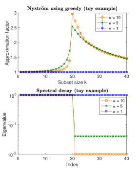
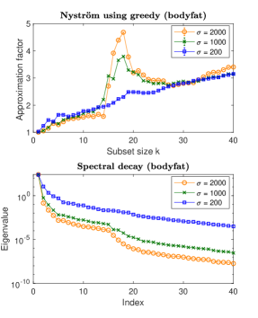
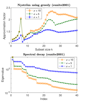
The plots in Figure 4 confirm that the Nyström approximation factor of greedy subset selection exhibits similar peaks and valleys as those indicated by our theoretical and empirical analysis of the k-DPP method. This is most clearly observed for the toy dataset (Figure 4 left), where the peak grows with the condition number $\kappa$, and for the bodyfat dataset (Figure 4 center), where the size of the peak is proportional to the RBF parameter $\sigma$. Moreover, we observe that when the spectral decay is slow/smooth, which corresponds to smaller values of $\sigma$, then the approximation factor of the greedy algorithm stays relatively close to 1. For the eunite2001 dataset (Figure 4 right), the behavior of the approximation factor is very non-linear, with several peaks occurring for large values of $\sigma$. Interestingly, while the peaks do align with some of the drops in the spectrum, not all of the spectrum drops result in a peak for the greedy algorithm. This goes in line with our analysis, in the sense that a sharp drop in the spectrum following the $k$th eigenvalue is a necessary but not sufficient condition for the approximation factor of the optimal subset $S$ of size $k$ to exhibit a peak.

Our empirical evaluation leads to an overall conclusion that the multiple-descent curve of the CSSP/Nyström approximation factor is a phenomenon exhibited by both randomized methods, such as the k-DPP, and deterministic algorithms, such as greedy subset selection. While the exact behavior of this curve is algorithm-dependent, significant insight can be gained about it by studying the spectral properties of the data. Our results suggest that performing a theoretical analysis of the multiple-descent phenomenon for greedy methods is a promising direction for future work.

References

• Alaoui & Mahoney (2015) Alaoui, A. E. and Mahoney, M. W. Fast randomized kernel ridge regression with statistical guarantees. In Proceedings of the 28th International Conference on Neural Information Processing Systems, pp.  775–783, Montreal, Canada, December 2015.
• Altschuler et al. (2016) Altschuler, J., Bhaskara, A., Fu, G., Mirrokni, V., Rostamizadeh, A., and Zadimoghaddam, M. Greedy column subset selection: New bounds and distributed algorithms. In Balcan, M. F. and Weinberger, K. Q. (eds.), Proceedings of The 33rd International Conference on Machine Learning, volume 48 of Proceedings of Machine Learning Research, pp.  2539–2548, New York, New York, USA, 20–22 Jun 2016. PMLR.
• Anari et al. (2016) Anari, N., Gharan, S. O., and Rezaei, A. Monte carlo markov chain algorithms for sampling strongly rayleigh distributions and determinantal point processes. In Feldman, V., Rakhlin, A., and Shamir, O. (eds.), 29th Annual Conference on Learning Theory, volume 49 of Proceedings of Machine Learning Research, pp.  103–115, Columbia University, New York, New York, USA, 23–26 Jun 2016. PMLR.
• Avron & Boutsidis (2013) Avron, H. and Boutsidis, C. Faster subset selection for matrices and applications. SIAM Journal on Matrix Analysis and Applications, 34(4):1464–1499, 2013.
• Bach & Jordan (2003) Bach, F. R. and Jordan, M. I. Kernel independent component analysis. J. Mach. Learn. Res., 3:1–48, March 2003. ISSN 1532-4435.
• Balzano et al. (2010) Balzano, L., Recht, B., and Nowak, R. High-dimensional matched subspace detection when data are missing. In 2010 IEEE International Symposium on Information Theory, pp.  1638–1642. IEEE, 2010.
• Bartlett et al. (2019) Bartlett, P. L., Long, P. M., Lugosi, G., and Tsigler, A. Benign overfitting in linear regression. Technical Report Preprint: arXiv:1906.11300, 2019.
• Belabbas & Wolfe (2009) Belabbas, M.-A. and Wolfe, P. J. Spectral methods in machine learning and new strategies for very large datasets. Proceedings of the National Academy of Sciences, 106(2):369–374, 2009. ISSN 0027-8424. doi: 10.1073/pnas.0810600105.
• Belhadji et al. (2018) Belhadji, A., Bardenet, R., and Chainais, P. A determinantal point process for column subset selection. arXiv e-prints, art. arXiv:1812.09771, Dec 2018.
• Belkin et al. (2019a) Belkin, M., Hsu, D., Ma, S., and Mandal, S. Reconciling modern machine-learning practice and the classical bias–variance trade-off. Proc. Natl. Acad. Sci. USA, 116:15849–15854, 2019a.
• Belkin et al. (2019b) Belkin, M., Hsu, D., and Xu, J. Two models of double descent for weak features. arXiv preprint arXiv:1903.07571, 2019b.
• Boutsidis & Woodruff (2014) Boutsidis, C. and Woodruff, D. P. Optimal CUR matrix decompositions. In Proceedings of the Forty-Sixth Annual ACM Symposium on Theory of Computing, STOC ’14, pp.  353–362, New York, NY, USA, 2014. Association for Computing Machinery. ISBN 9781450327107.
• Boutsidis et al. (2008) Boutsidis, C., Mahoney, M., and Drineas, P. An improved approximation algorithm for the column subset selection problem. Proceedings of the Annual ACM-SIAM Symposium on Discrete Algorithms, 12 2008.
• Boutsidis et al. (2011) Boutsidis, C., Drineas, P., and Magdon-Ismail, M. Near optimal column-based matrix reconstruction. In 2011 IEEE 52nd Annual Symposium on Foundations of Computer Science, pp.  305–314, Oct 2011.
• Burt et al. (2019) Burt, D., Rasmussen, C. E., and Van Der Wilk, M. Rates of convergence for sparse variational Gaussian process regression. In Chaudhuri, K. and Salakhutdinov, R. (eds.), Proceedings of the 36th International Conference on Machine Learning, volume 97 of Proceedings of Machine Learning Research, pp.  862–871, Long Beach, California, USA, 09–15 Jun 2019. PMLR.
• Calandriello et al. (2020) Calandriello, D., Dereziński, M., and Valko, M. Sampling from a $k$-dpp without looking at all items. arXiv preprint arXiv:2006.16947, 2020. Accepted for publication, Proc. NeurIPS 2020.
• Chan & Hansen (1992) Chan, T. F. and Hansen, P. C. Some applications of the rank revealing QR factorization. SIAM Journal on Scientific and Statistical Computing, 13(3):727–741, 1992.
• Chang & Lin (2011) Chang, C.-C. and Lin, C.-J. LIBSVM: A library for support vector machines. ACM Transactions on Intelligent Systems and Technology, 2:27:1–27:27, 2011.
• Chierichetti et al. (2017) Chierichetti, F., Gollapudi, S., Kumar, R., Lattanzi, S., Panigrahy, R., and Woodruff, D. P. Algorithms for $\ell_{p}$ low-rank approximation. volume 70 of Proceedings of Machine Learning Research, pp. 806–814, International Convention Centre, Sydney, Australia, 06–11 Aug 2017. PMLR.
• Chung & Lu (2006) Chung, F. and Lu, L. Complex Graphs and Networks (Cbms Regional Conference Series in Mathematics). American Mathematical Society, Boston, MA, USA, 2006. ISBN 0821836579.
• Dereziński (2019) Dereziński, M. Fast determinantal point processes via distortion-free intermediate sampling. In Beygelzimer, A. and Hsu, D. (eds.), Proceedings of the Thirty-Second Conference on Learning Theory, volume 99 of Proceedings of Machine Learning Research, pp.  1029–1049, Phoenix, USA, 25–28 Jun 2019.
• Dereziński & Mahoney (2020) Dereziński, M. and Mahoney, M. W. Determinantal point processes in randomized numerical linear algebra. arXiv preprint arXiv:2005.03185, 2020. Accepted for publication, Notices of the AMS.
• Dereziński & Warmuth (2018) Dereziński, M. and Warmuth, M. K. Reverse iterative volume sampling for linear regression. Journal of Machine Learning Research, 19(23):1–39, 2018.
• Dereziński et al. (2019) Dereziński, M., Calandriello, D., and Valko, M. Exact sampling of determinantal point processes with sublinear time preprocessing. In Wallach, H., Larochelle, H., Beygelzimer, A., d Alché-Buc, F., Fox, E., and Garnett, R. (eds.), Advances in Neural Information Processing Systems 32, pp.  11542–11554. Curran Associates, Inc., 2019.
• Dereziński et al. (2019a) Dereziński, M., Clarkson, K. L., Mahoney, M. W., and Warmuth, M. K. Minimax experimental design: Bridging the gap between statistical and worst-case approaches to least squares regression. In Beygelzimer, A. and Hsu, D. (eds.), Proceedings of the Thirty-Second Conference on Learning Theory, volume 99 of Proceedings of Machine Learning Research, pp.  1050–1069, Phoenix, USA, 25–28 Jun 2019a.
• Dereziński et al. (2019b) Dereziński, M., Liang, F., and Mahoney, M. W. Exact expressions for double descent and implicit regularization via surrogate random design. arXiv preprint arXiv:1912.04533, 2019b. Accepted for publication, Proc. NeurIPS 2020.
• Dereziński et al. (2020) Dereziński, M., Liang, F., and Mahoney, M. Bayesian experimental design using regularized determinantal point processes. In International Conference on Artificial Intelligence and Statistics, pp.  3197–3207, 2020.
• Deshpande & Rademacher (2010) Deshpande, A. and Rademacher, L. Efficient volume sampling for row/column subset selection. In Proceedings of the 2010 IEEE 51st Annual Symposium on Foundations of Computer Science, pp.  329–338, Las Vegas, USA, October 2010.
• Deshpande et al. (2006) Deshpande, A., Rademacher, L., Vempala, S., and Wang, G. Matrix approximation and projective clustering via volume sampling. In Proceedings of the Seventeenth Annual ACM-SIAM Symposium on Discrete Algorithm, pp.  1117–1126, Miami, FL, USA, January 2006.
• Drineas & Mahoney (2005) Drineas, P. and Mahoney, M. W. On the Nyström method for approximating a Gram matrix for improved kernel-based learning. Journal of Machine Learning Research, 6:2153–2175, 2005.
• Drineas et al. (2008) Drineas, P., Mahoney, M. W., and Muthukrishnan, S. Relative-error CUR matrix decompositions. SIAM Journal on Matrix Analysis and Applications, 30(2):844–881, 2008.
• Elenberg et al. (2018) Elenberg, E. R., Khanna, R., Dimakis, A. G., and Negahban, S. Restricted Strong Convexity Implies Weak Submodularity. Annals of Statistics, 2018.
• Gautier et al. (2019) Gautier, G., Polito, G., Bardenet, R., and Valko, M. DPPy: DPP Sampling with Python. Journal of Machine Learning Research - Machine Learning Open Source Software (JMLR-MLOSS), in press, 2019. Code at http://github.com/guilgautier/DPPy/ Documentation at http://dppy.readthedocs.io/.
• Gittens & Mahoney (2016) Gittens, A. and Mahoney, M. W. Revisiting the Nyström method for improved large-scale machine learning. J. Mach. Learn. Res., 17(1):3977–4041, January 2016. ISSN 1532-4435.
• Gong et al. (2014) Gong, B., Chao, W.-L., Grauman, K., and Sha, F. Diverse sequential subset selection for supervised video summarization. In Ghahramani, Z., Welling, M., Cortes, C., Lawrence, N. D., and Weinberger, K. Q. (eds.), Advances in Neural Information Processing Systems 27, pp.  2069–2077. Curran Associates, Inc., 2014.
• Gu & Eisenstat (1996) Gu, M. and Eisenstat, S. C. Efficient algorithms for computing a strong rank-revealing qr factorization. SIAM Journal on Scientific Computing, 17(4):848–869, 1996.
• Guruswami & Sinop (2012) Guruswami, V. and Sinop, A. K. Optimal column-based low-rank matrix reconstruction. In Proceedings of the Twenty-third Annual ACM-SIAM Symposium on Discrete Algorithms, pp.  1207–1214, Kyoto, Japan, January 2012.
• Guyon & Elisseeff (2003) Guyon, I. and Elisseeff, A. An introduction to variable and feature selection. J. Mach. Learn. Res., 3(null):1157–1182, March 2003. ISSN 1532-4435.
• Hardy et al. (1952) Hardy, G., Littlewood, J., and Pólya, G. Inequalities. Cambridge University Press, 2nd edition, 1952.
• Hough et al. (2006) Hough, J. B., Krishnapur, M., Peres, Y., Virág, B., et al. Determinantal processes and independence. Probability surveys, 3:206–229, 2006.
• Khanna et al. (2017) Khanna, R., Elenberg, E. R., Dimakis, A. G., Neghaban, S., and Ghosh, J. Scalable greedy support selection via weak submodularity. Proceedings of the International Conference on Artificial Intelligence and Statistics (AISTATS), pp.  1560–1568, 2017.
• Kim et al. (2016) Kim, B., Khanna, R., and Koyejo, O. Examples are not enough, learn to criticize! criticism for interpretability. In Advances in Neural Information Processing Systems, 2016.
• Kulesza & Taskar (2011) Kulesza, A. and Taskar, B. k-DPPs: Fixed-Size Determinantal Point Processes. In Proceedings of the 28th International Conference on Machine Learning, pp.  1193–1200, June 2011.
• Kulesza & Taskar (2012) Kulesza, A. and Taskar, B. Determinantal Point Processes for Machine Learning. Now Publishers Inc., Hanover, MA, USA, 2012.
• Lawlor et al. (2016) Lawlor, D., Budavári, T., and Mahoney, M. W. Mapping the similarities of spectra: Global and locally-biased approaches to SDSS galaxy data. Astrophysical Journal, 833(1), 12 2016.
• Liang et al. (2020) Liang, T., Rakhlin, A., and Zhai, X. On the multiple descent of minimum-norm interpolants and restricted lower isometry of kernels. arXiv preprint arXiv:1908.10292 [cs, math, stat], 2020.
• Liao et al. (2020) Liao, Z., Couillet, R., and Mahoney, M. W. A random matrix analysis of random fourier features: beyond the gaussian kernel, a precise phase transition, and the corresponding double descent. arXiv preprint arXiv:2006.05013, 2020. Accepted for publication, Proc. NeurIPS 2020.
• Macchi (1975) Macchi, O. The coincidence approach to stochastic point processes. Advances in Applied Probability, 7(1):83–122, 1975. ISSN 00018678.
• Mahoney (2012) Mahoney, M. W. Approximate computation and implicit regularization for very large-scale data analysis. In Proceedings of the 31st ACM Symposium on Principles of Database Systems, pp.  143–154, 2012.
• Musco & Musco (2017) Musco, C. and Musco, C. Recursive sampling for the nystrom method. In Guyon, I., Luxburg, U. V., Bengio, S., Wallach, H., Fergus, R., Vishwanathan, S., and Garnett, R. (eds.), Advances in Neural Information Processing Systems 30, pp.  3833–3845. Curran Associates, Inc., 2017.
• Mutny et al. (2020) Mutny, M., Dereziński, M., and Krause, A. Convergence analysis of block coordinate algorithms with determinantal sampling. In International Conference on Artificial Intelligence and Statistics, pp.  3110–3120, 2020.
• Paul et al. (2015) Paul, S., Magdon-Ismail, M., and Drineas, P. Column selection via adaptive sampling. In Proceedings of the 28th International Conference on Neural Information Processing Systems - Volume 1, NIPS’15, pp.  406–414, Cambridge, MA, USA, 2015. MIT Press.
• Poggio et al. (2019) Poggio, T., Kur, G., and Banburski, A. Double descent in the condition number. arXiv preprint, arXiv:1912.06190, 2019.
• Rasmussen & Williams (2006) Rasmussen, C. E. and Williams, C. K. I. Gaussian Processes for Machine Learning. MIT Press, 2006.
• Roughgarden (2019) Roughgarden, T. Beyond worst-case analysis. Communications of the ACM, 62(3):88–96, 2019.
• Santa et al. (1997) Santa, H. Z., Zhu, H., Williams, C. K. I., Rohwer, R., and Morciniec, M. Gaussian regression and optimal finite dimensional linear models. In Neural Networks and Machine Learning, pp.  167–184. Springer-Verlag, 1997.
• Wang et al. (2019) Wang, R., Li, Y., Mahoney, M. W., and Darve, E. Block basis factorization for scalable kernel evaluation. SIAM Journal on Matrix Analysis and Applications, 40(4):1497–1526, 2019.
• Warlop et al. (2019) Warlop, R., Mary, J., and Gartrell, M. Tensorized determinantal point processes for recommendation. In Proceedings of the 25th ACM SIGKDD International Conference on Knowledge Discovery & Data Mining, KDD ’19, pp.  1605–1615, New York, NY, USA, 2019. ACM. ISBN 978-1-4503-6201-6.
• Williams & Seeger (2001) Williams, C. K. I. and Seeger, M. Using the Nyström method to speed up kernel machines. In Leen, T. K., Dietterich, T. G., and Tresp, V. (eds.), Advances in Neural Information Processing Systems 13, pp.  682–688. MIT Press, 2001.