Spectra of chains connected to complete graphs

Abstract

We characterize the spectrum of the Laplacian of graphs composed of one or two finite or infinite chains connected to a complete graph. We show the existence of localized eigenvectors of two types, eigenvectors that vanish exactly outside the complete graph and eigenvectors that decrease exponentially outside the complete graph. Our results also imply gaps between the eigenvalues corresponding to localized and extended eigenvectors.

1 Introduction

We study the spectrum of the Laplacian of finite and infinite graphs obtained by joining complete graphs and chains. We focus on the existence and properties of eigenvectors that are localized in the nodes of the complete graph.

Our work is motivated by studies of linear and nonlinear mass-spring models of protein vibrations, where the interaction between the amino-acids of the protein is encoded in a graph [1, 14, 6, 11]. It has been suggested that oscillations localized in small subregions of certain types of proteins, particularly enzymes, play a significant biochemical role, see references in [13, 4]. Moreover, such oscillations occur in regions of higher density of the protein, where amino-acids interact with a larger number of neighboring amino-acids [6, 13]. The linear modes and frequencies of mass-spring models are connected to the eigenvectors and eigenvalues of the Laplacian of the graph describing the connectivity of the masses, see [11]. Information on the frequencies and shape of the localized eigenvectors can be used to investigate weakly nonlinear modes [9, 11, 10].

The above considerations justify the study of the spectrum of the Laplacian of graphs that have the geometry of proteins. In [11, 10] we showed how localization in complete graphs connected to chain graphs suggests a mechanism of localization in proteins. In the present work we consider some of the simplest examples of complete graphs connected to chains in order to obtain detailed information. We plan to use this information in a constructive approach to study more complicated graphs related to proteins.

We study first the Laplacian of a complete graph of $p\geq 6$ nodes joined to a chain of $q\geq 3$ nodes and show the existence of $p-2$ eigenvectors with support in the complete graph component, these are referred to as “clique eigenvectors”. The clique eigenvectors are degenerate and have eigenvalue $p$, see Proposition 3.3. We also show the existence of an eigenvector that decays outside the complete graph nodes and corresponds to an eigenvalue in the interval $(p,p+2)$, see Proposition 3.10. This localized eigenvector, referred to as an “edge eigenvector”, has its maximum amplitude at the node connecting the complete graph to the chain and decays exponentially (up to a small error) in the chain. Our analysis also gives the decay rate of the edge eigenvectors and asymptotics for large $p$. The remaining eigenvalues are in $[0,4]$. The corresponding eigenvectors, referred to as “chain eigenvectors”, have small amplitude in the nodes of the complete graph. Similar statements apply to the case where $p\geq 6$, and $q=\infty$, see Propositions 3.4, and 3.6. The results on clique and edge eigenvectors and their eigenvalues are similar to the ones obtained for finite chains. The spectrum includes the interval $[0,4]$, corresponding to oscillatory nondecaying generalized eigenvectors.

We also analyze the spectrum of a complete graph of $p\geq 5$ nodes joined to two chains of $q_{1}$, $q_{2}\geq 3$ nodes respectively. We show the existence of $p-3$ clique eigenvectors and two edge eigenvectors, see Propositions 4.2, 4.9. In the case $q_{1}=q_{2}=q$ we have one symmetric and one antisymmetric edge eigenvector. The remaining eigenvalues are in $[0,4]$ and correspond to chain eigenvectors. For $q_{1}=q_{2}=\infty$ we have similar results for the localized states, see Propositions 4.3, 4.4, with one symmetric and one antisymmetric edge eigenvector. The spectrum includes the interval $[0,4]$.

The constructive proofs of the edge eigenvectors for both finite and infinite chains start with an exact computation of the clique eigenvectors. The eigenvectors normal to the clique eigenvectors are examined by interpreting the eigenvalue problem at the chain sites as a linear dynamical system, with additional conditions at the boundary of the chain. This analysis yields an algebraic equation for the edge eigenvalues. We obtain bounds for the edge eigenvalues by examining the roots of the algebraic equations. Note that the proofs for the one- and two-chain finite and infinite problems follow the same pattern. For two chains, the algebraic equations becomes more involved. The analysis can be simplified by symmetry or by using the Courant-Weyl estimates. We note that the Courant-Weyl estimates, Lemmas 3.2, 4.1, give a good approximation of the spectrum for finite graphs. The dynamical approach is independent and leads to more precise results.

We also present additional numerical and asymptotic results, for instance simplified expressions of the decay rate of edge eigenvectors for large $p$. We also note the possibility of embedded eigenvalues for small values of $p$. The results obtained for one or two chains connected to a complete graph suggest conjectures for the spectrum of a graph composed of many complete graphs connected by chains.

The article is organized as follows. Definitions and notation are presented in section 2. Sections 3 and 4 contain respectively the analysis for a complete graph connected to one and two chains. In Section 5 we present conjectures on the spectrum of a graph composed of many complete graphs connected by chains.

2 Definitions and Notation

A finite undirected graph $G=({\cal V},c)$ is defined by a set of vertices ${\cal V}\in\mathbb{Z}$ together with a connectivity function $c:{\cal V}\times{\cal V}\rightarrow\{0,-1\}$ satisfying $c_{ij}=-1$ if vertices $i,j$ are connected and $0$ otherwise. From the connectivity function, one can build the Laplacian matrix of $G$ with $|V|=n$ as the $n\times n$ matrix $L$ such that $L_{ij}=c_{ij}=-1$ if $ij$ is an edge and $L_{ii}=\sum_{j=1}^{n}L_{ij}$. We assume the graph to be connected $L_{ii}>0,\forall i$. The degree $d_{i}$ is the number of connections of vertex $i$.

Since $L$ is symmetric and nonnegative, its eigenvalues $\lambda_{k},k=1,\dots,n$ are real non negative and the eigenvectors $v^{k}$ can be chosen orthonormal. We can order the eigenvalues in the following way

$$\lambda_{1}\geq\lambda_{2}\geq\dots>\lambda_{n}=0.$$

Note that only $\lambda_{n}$ is zero because the graph is connected [5].

We also allow the graph to be infinite, so that $G=({\cal V},c)$ is a subset ${\cal V}$ of $\mathbb{Z}$ but assume a finite degree for each vertex.

We introduce some additional definitions for infinite graphs. Consider the standard Hermitian inner product $\langle f,g\rangle_{c}=\sum_{j\in{\cal I}}f_{j}g^{*}_{j}$, $f$, $g$ complex-valued functions on ${\cal V}$, and the corresponding space $l^{2}_{c}=l^{2}_{c}({\cal V};{\mathbb{C}})$ of $f$ satisfying $||f||^{2}_{l^{2}}=\langle f,f\rangle_{c}<\infty$. We also consider the space $l^{\infty}_{c}$ of functions $f$ satisfying $\sup_{j\in{\cal V}}|f_{j}|<\infty$. The real subspaces of real valued elements of $l^{2}_{c}$, $l^{\infty}_{c}$ will be denoted by $l^{2}$, $l^{\infty}$. The restriction of $\langle\cdot,\cdot\rangle_{c}$ to elements of $l^{2}\times l^{2}$ defines an inner product in $l^{2}$, denoted by $\langle\cdot,\cdot\rangle$.

Given a bounded linear operator $M$ in $l_{c}^{2}$, the residual set $\rho(M)$ of $M$ is the set of all $\lambda\in\mathbb{C}$ for which $M-\lambda I$ has a bounded inverse in $l^{2}_{c}$, $I$ the identity. The spectrum $\sigma(M)$ is the complement of $\rho(M)$ in $\mathbb{C}$. The point spectrum $\sigma_{p}(M)$ of $M$ is the set of all $\lambda\in\mathbb{C}$ satisfying $Mv=\lambda v$ for some $v$ in $l^{2}_{c}$. Such $v\in l^{2}_{c}$ are also denoted as eigenvectors of $M$. We have $\sigma_{p}(M)\subset\sigma(M)$. The Laplacian $L$ of a graph of finite degree is a bounded operator in $l^{2}_{c}$, and is also Hermitian, and nonnegative. We therefore have $\sigma(L)\subset[0,+\infty)$. By the reality of $L$, $\sigma(L)$, we may seek eigenvalues of $L$ in $l^{2}$.

In the case a finite graph, $\sigma(L)=\sigma_{p}(L)$, i.e. the set of eigevalues above. In the case of infinite graphs, the spectrum of $L$ may be larger than the point spectrum. We use the notion of the essential spectrum $\sigma_{e}(M)$ of a bounded operator $M$ in $l^{2}_{c}$ defined as in [7], p.29, namely $\lambda\in\sigma(M)$ belongs to $\sigma_{e}(M)$ if $M-\lambda I$ either fails to be Fredholm, or is Fredholm with nonzero index, see e.g. [8], p.243, for a weaker condition, namely $M-\lambda I$ not semi-Fredholm.

In the case of the graphs studied below we see examples of $u\in l^{\infty}_{c}$, $u\notin l^{2}_{c}$, that satisfy $Lu=\lambda u$. Such $\lambda$, and $u$ may be referred to as generalized eigenvalues and eigenvectors of $L$ respectively. We can show that such $\lambda$ belong to $\sigma_{e}(L)$, see e.g. [7], ch. 1. Also, we see examples of graphs for which $\sigma_{e}(L)\cap\sigma_{p}(L)\neq\emptyset$, the corresponding eigenvalues may be referred to embedded eigenvalues. We may distinguish cases where we have elements in $\sigma_{p}(L)$ is in the interior or the boundary of $\sigma_{e}(L)$.

We recall the standard definitions of a chain and a clique, together with well-known properties.

Definition 2.1

A chain $C_{q}$ is a connected graph of $q-1$ vertices whose Laplacian $L$ is a tri-diagonal matrix.

The eigenvalues of the Laplacian of $C_{q}$ are given by

$$\lambda_{j}=4\sin^{2}\left[\frac{\pi(q-1)-j}{2(q-1)}\right],\quad j=1,\ldots,q-1.$$ (2.1)

Definition 2.2

A clique, $K_{n}$ is a complete graph with $n$ vertices. Its Laplacian has $n$ on the diagonal $n$ and all other entries are equal to $-1$.

The spectrum of a clique $K_{n}$ is well-known [5], we have

Property 2.3

A clique $K_{n}$ has eigenvalue $n$ with multiplicity $n-1$ and eigenvectors $v^{k}=(1,0,\dots,0,-1,0,\dots,0,)^{T},~{}~{}~{}k=1,\dots,n-1$ and eigenvalue $0$ for the constant eigenvector $v^{n}$.

2.1 A chain connected to a clique

We consider graphs formed by the association of clique $K_{p}$ and a chain $C_{q}$ denoted by $G=K_{p}\oplus C_{q}$, with $p\geq 3$, $q\geq 2$ positive integers, defined by the set

$${\cal V}={\cal V}_{p,-}\cup{\cal V}_{q,+},\quad{\cal V}_{p,-}=\{-p+1,-p+2,\ldots,0\},\quad{\cal V}_{q,+}=\{1,2,\ldots,q-1\},$$ (2.2)

and a connectivity matrix $c$ that satisfies

$$c_{ij}=-1,\quad\forall i,j\in{\cal V}_{p,-},$$ (2.3)

$$c_{01}=c_{10}=-1,$$ (2.4)

$$c_{ij}=-1,\quad\forall i,j\in{\cal V}_{q,+}\quad\hbox{with}\quad|i-j|=1,$$ (2.5)

and $c_{ij}=0$ for all other pairs $(i,j)\in{\cal V}\times{\cal V}$. Equations (2.3)-(2.5) describe a complete graph of $p$ nodes, the set ${\cal V}_{p,-}$, joined to a chain of $q$ nodes, the set ${\cal V}_{q,+}$ with nearest-neighbor connectivity (2.5). The two sets are joined by (2.4).

Property 2.4

The Laplacian of a graph composed of a complete graph of $p$ nodes joined joined to a chain of $q$ nodes is

$$L=L^{\prime}_{K_{p}}+L^{\prime}_{C_{q}},$$

where $L^{\prime}_{C_{q}}$ is the augmented Laplacian of the chain $C_{q}$, $L^{\prime}_{C_{q}}=\begin{pmatrix}0&0\\ 0&L_{C_{q}}\\ \end{pmatrix}$ and similarly $L^{\prime}_{K_{p}}=\begin{pmatrix}L_{K_{p}}&0\\ 0&0\\ \end{pmatrix}$.

We then write the graph as $K_{p}\oplus C_{q}$.

2.2 A motivational example

We consider the graph $K_{6}\oplus C_{4}$ shown in Fig. 1.

Figure 1: A chain 3 coupled to the clique K₆

The Laplacian is

$$L=L_{C_{4}}+L_{K_{6}}=\begin{pmatrix}5&-1&-1&-1&-1&-1&.&.&.\\ -1&5&-1&-1&-1&-1&.&.&.\\ -1&-1&5&-1&-1&-1&.&.&.\\ -1&-1&-1&5&-1&-1&.&.&.\\ -1&-1&-1&-1&5&-1&.&.&.\\ -1&-1&-1&-1&-1&6&-1&.&.\\ .&.&.&.&.&-1&2&-1&.\\ .&.&.&.&.&.&-1&2&-1\\ .&.&.&.&.&.&.&-1&1\\ \end{pmatrix},$$ (2.6)

where $L_{C_{4}}$ is the Laplacian of an $n=9$ vertex graph such that the last 4 vertices form a chain $q=4$, $L_{K_{6}}$ is the Laplacian of an $n=9$ vertex graph such that the first 6 vertices form a clique $p=6$ and where the $0$’s are represented by . for clarity.

The eigenvectors and corresponding eigenvalues are

node	$v^{1}$	$v^{2}$	$v^{3}$	$v^{4}$	$v^{5}$	$v^{6}$	$v^{7}$	$v^{8}$	$v^{9}$
1	0.1524	0	0	0	0	-0.04879	0.098934	-0.23129	0.33333
2	0.1524	-0.707	0	0.707	0	-0.04879	0.098934	-0.23129	0.33333
3	0.1524	0	0.707	-0.707	0	-0.04879	0.098934	-0.23129	0.33333
4	0.1524	0.707	0	0	0.707	-0.04879	0.098934	-0.23129	0.33333
5	0.1524	0	-0.707	0	-0.707	-0.04879	0.098934	-0.23129	0.33333
6	-0.9198	0	0	0	0	0.10652	-0.051079	-0.16999	0.33333
7	0.19043	0	0	0	0	0.54399	-0.72369	0.18156	0.33333
8	-0.039105	0	0	0	0	-0.75017	-0.29898	0.48499	0.33333
9	0.0064791	0	0	0	0	0.34361	0.57908	0.65988	0.33333
$\lambda$	7.0355	6	6	6	6	3.1832	1.5163	0.26503	0

Table 1: Eigenvectors and eigenvalues for the graph $G=C_{4}\oplus K_{6}$.

We see that $p-1=4$ of the $p=5$ eigenvalues of K₆ are preserved. This is easy to see by padding with zeros 4 eigenvectors of K₆

$$v^{2}=(0;0;0;-1;1;0;0;0;0)^{T},~{}~{}v^{3}=(0;1;-1;0;0;0;0;0;0)^{T},$$

$$v^{4}=(0;0;1;0;-1;0;0;0;0)^{T},~{}~{}v^{5}=(0;-1;0;1;0;0;0;0;0)^{T}$$

The five other eigenvectors $\{v^{1},v^{6},v^{7},v^{8},v^{9}\}$ have the property that

$$v_{k}^{i}=x^{i},~{}~{}k<4,$$ (2.7)

because these eigenvectors need to be orthogonal to the eigenvectors of the clique $\{v^{2},v^{3},v^{4},v^{5}\}$. They are then constant in the clique section of the graph $k<4$ except at the junction vertex.

For the graph studied above, these eigenvectors are plotted in Fig. 2.

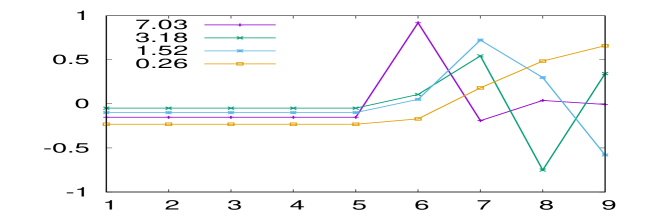
Figure 2: Plot of the eigenvectors $\{v^{1},v^{6},v^{7},v^{8}\}$ corresponding to eigenvalues $7.03,~{}3.18,~{}1.52,~{}0.26$.

In the article, we prove the results illustrated in this example, specifically

• the existence of $p-2$ ”clique” eigenvalues $p$ for a graph $G=K_{p}\oplus C_{q}$. The corresponding eigenvectors are non zero in the clique region only.

• the existence of one ”edge” eigenvalue, strictly larger than $p$, constant in the clique region and decaying in the chain region.

• the existence of two ”edge” eigenvalues, strictly larger than $p$ for a clique $K_{p}$ connected to two chains $C_{q_{1}},C_{q_{2}}$.

3 A chain connected to a clique

We study the graph $K_{p}\oplus C_{q}$. First, we use the relation for the Laplacian of $K_{p}\oplus C_{q}$

$$L_{K_{p}\oplus C_{q}}=L^{\prime}_{K_{p}}+L^{\prime}_{C_{q}}$$

and the Courant-Weyl inequalities on the sum of two Hermitian matrices to obtain bounds on the eigenvalues of $K_{p}\oplus C_{q}$.

3.1 Courant-Weyl inequalities

We have the following Courant-Weyl inequalities, see e.g. [2].

Proposition 3.1

Let $A$, $B$ symmetric $n\times n$ matrices, then the Weyl inequalities are

$$\lambda_{k_{1}}(A)+\lambda_{k_{2}}(B)\leq\lambda_{i}(A+B)\leq\lambda_{j_{1}}(A)+\lambda_{j_{2}}(B),$$ (3.1)

for all $i=1,\ldots,n$, and all $k_{1}$, $k_{2}$, $j_{1}$, $j_{2}\in\{1,\ldots,n\}$ satisfying $k_{1}+k_{2}=n+i$ and $j_{1}+j_{2}=i+1$.

For $A$, $B$ nonnegative this also implies

$$\lambda_{i}(A)\leq\lambda_{i}(A+B)\leq\lambda_{j_{1}}(A)+\lambda_{j_{2}}(B),$$ (3.2)

for all $i=1,\ldots,n$, and all $j_{1},j_{2}\in\{1,\ldots,n\}$ satisfying $j_{1}+j_{2}=i+1$ .

Lemma 3.2

Let $L$ be the graph Laplacian of the graph $K_{p}\oplus C_{q}$, $p\geq 4$, $q\geq 4$. Then $\lambda_{1}(L)\in[p,p+2]$, and $\lambda_{j}(L)=p$, $\forall j\in\{2,\ldots,p-1\}$. Also $\lambda_{p}(L)\in(0,\hbox{min}\{\lambda_{1}(L_{C_{q}})+2,p\})$ ($\subset(0,p)$ if $p\geq 6$), and $\lambda_{j}(L)\in[0,4)$, $\forall j\in\{p+1,\ldots,p+q-1\}$.

Proof. We will apply the Weyl inequalities (3.2) using the decomposition $L=A+B$, where $A$ is the $(p+q+1)\times(p+q+1)$ block diagonal matrix with blocks $L_{K_{p}}$ and $L_{C_{q}}$. The only non-vanishing elements of $B$ are $B(p,p)=B(p+1,p+1)=1$, $B(p+1,p)=B(p,p+1)=-1$.

We then have $\lambda_{j}(A)=p$ if $j\in\{1,\ldots,p-1\}$, and $\lambda_{p-1+k}(A)=\lambda_{k}(L_{C_{q}})\in(0,4)$ for $k\in\{1,q-2\}$. Also $\lambda_{p+q-2}(A)=\lambda_{p+q-1}(A)=0$. In addition, $\lambda_{1}(B)=2$, and $\lambda_{j}(B)=0$, $\forall j\in\{2,\ldots,p+q-1\}$.

We use $\lambda_{j}(A)\leq\lambda_{j}(A+B)$, $j=1,\ldots,p+q-1$, see (3.2), as lower bounds.

For the upper bounds we first note that

$$\lambda_{1}(A+B)\leq\lambda_{1}(A)+\lambda_{1}(B)=p+2.$$

For $j\in{2,\ldots,p-1\ }$ we have

$$\lambda_{j}(A+B)\leq\hbox{min}\{\lambda_{j}(A)+\lambda_{1}(B),\ldots,\lambda_{1}(A)\}=p,$$

since $\lambda_{j}(B)=0$, $\forall j\in\{2,\ldots,p+q-1\}$. Similarly

$$\lambda_{p}(A+B)\leq\hbox{min}\{\lambda_{p}(A)+\lambda_{1}(B),\ldots,\lambda_{1}(A)\}=\hbox{min}\{\lambda_{1}(L_{C_{q}})+2,p\}.$$

In the case $p\geq 6$ we also have $\lambda_{1}(L_{C_{q}})+2<6\leq p$, therefore $\lambda_{p}(A+B)<p$.

For $j\in\{p+1,\ldots,p+q-1\}$, i.e. $j=p-1+k$, $k\in\{2,\ldots,q-2\}$, we have

$$\lambda_{p-1+k}(A+B) \leq \hbox{min}\{\lambda_{k}(L_{C_{q}})+\lambda_{1}(B),\lambda_{k-1}(L_{C_{q}}),\ldots,\lambda_{1}(A)\}$$

$$= \hbox{min}\{\lambda_{k}(L_{C_{q}})+2,\lambda_{k-1}(L_{C_{q}})\}<4$$

using $\lambda_{k-1}(L_{C_{q}})<4<p$. Also $\lambda_{p+q-2}(A+B)\leq\min\{2,\lambda_{{\tilde{q}}-1}(L_{C_{q}})\}<4$, and $\lambda_{p+q-1}(A+B)=0$. The statement follows by combining the above with the lower bounds. $\Box$

3.2 Clique eigenvectors

We show the existence of eigenvectors that are strictly zero outside the clique component $K_{p}$.

Proposition 3.3

Let $L$ be the Laplacian of the graph $K_{p}\oplus C_{q}$, $p\geq 3$, $q\geq 1$. Then there exists a subspace $E_{K}$ of dimension $p-2$ such that $v\in E_{K}$ satisfies $Lv=pv$, and $v_{j}=0$, $\forall j\notin\{-p+1,\ldots,-1\}$.

Proof. Let $k\in\{2,\ldots,p-1\}$ and define the vectors $v^{k}\in l^{2}$ by

$$v^{k}_{-1}=1,\quad v^{k}_{-k}=-1,\quad v^{k}_{j}=0,\quad\forall j\in{\cal V}\setminus\{-1,-k\}.$$ (3.3)

We check that the $v^{k}$ are linearly independent. The statement follows by checking that $Lv^{k}=pv^{k}$, $\forall k\in\{2,\ldots,p-1\}$. Consider first $i\geq 1$. Then

$$(Lv^{k})_{i}=\sum_{j\in\{-1,-k\}}L_{i,j}v^{k}_{j}=0=pv^{k}_{i}$$ (3.4)

since $L_{ij}=c_{ij}=0$ if $i\geq 1$, $j\leq-1$ by (2.3)-(2.5). In the case $i\in\{-(p-1),\ldots,0\}\setminus\{-1,-k\}$ we have

$$(Lv^{k})_{i} = \sum_{j\in\{-1,-k\}}L_{ij}v^{k}_{j}$$ (3.5)

$$= L_{i,-1}-L_{i,-k}=c_{i,-1}-c_{i,-k}=0=pv^{k}_{i},$$

by (3.3), (2.3)-(2.5). Also,

$$(Lv^{k})_{-1} = \sum_{j\in\{-1,-k\}}L_{-1,j}v^{k}_{j}$$ (3.6)

$$= L_{-1,-1}-L_{-1,-k}=(p-1)+1=p=pv^{k}_{-1},$$

and

$$(Lv^{k})_{-k} = \sum_{j\in\{-1,-k\}}L_{-k,j}v^{k}_{j}$$ (3.7)

$$= L_{-k,-1}-L_{-k,-k}=-1+(-(p-1))=-p=pv^{k}_{-k}.$$

$\Box$

An alternative proof follows from noticing that the eigenvectors of $K_{p}$ that vanish at the sites connecting $K_{p}$ to the rest of the graph can be padded with zeros to form eigenvectors of $K_{p}\oplus C_{q}$, see [3] and [12].

The result extends to the case $q=\infty$:

Proposition 3.4

Let $L$ be the Laplacian of the graph $K_{p}\oplus C_{\infty}$, $p\geq 3$. Then there exists a subspace $E_{K}\in l^{2}$ of dimension $p-2$ such that $v\in E_{K}$ satisfies $Lv=pv$, and $v_{j}=0$, $\forall j\notin\{-p+1,\ldots,-1\}$.

The result follows by noticing that the clique eigenvectors of finite chains $K_{p}\oplus C_{q}$ can be extended to be eigenvectors of $K_{p}\oplus C_{\infty}$ by padding the sites beyond $q$ with zeros.

The next result is the existence of an “edge eigenvector”, that is constant on the nodes of $K_{p}$ and decays exponentially in the chain component.

Let $E$ be a real subspace of $l^{2}$, then $E^{\perp}$ denotes its orthogonal complement with respect to $\langle\cdot,\cdot\rangle$.

3.3 Edge eigenvector for a clique connected to an infinite chain

We first introduce the transfer matrix formalism used to simplify the problem in graphs that contain chains.

3.3.1 Transfer matrix for a chain

The equation $Lv=\lambda v$ for the infinite chain ${\cal V}=\mathbb{Z}$ with $c_{ij}=-1$ if $|i-j|=1$, $c_{ij}=0$ otherwise, is

$$-v_{j-1}+2v_{j}-v_{j+1}=\lambda v_{j},\quad\forall j\in\mathbb{Z}.$$ (3.8)

Define $M_{\lambda}$, $\lambda\in{\mathbb{R}}$, and $z_{j}$ by

$$M_{\lambda}=\left[\begin{array}[]{cc}0&1\\ -1&-\lambda+2\end{array}\right],~{}~{}z_{j}=\begin{pmatrix}v_{j}\\ v_{j+1}\end{pmatrix}.$$ (3.9)

Then (3.8) is equivalent to

$$z_{j+1}=M_{\lambda}z_{j},\quad\forall j\in\mathbb{Z}.$$ (3.10)

The eigenvalues $\sigma$ of $M_{\lambda}$ satisfy

$$\sigma^{2}-(-\lambda+2)\sigma+1=0,$$

they are

$$\sigma_{\pm}=\frac{1}{2}[(-\lambda+2)\pm\sqrt{(-\lambda+2)^{2}-4}].$$ (3.11)

The corresponding eigenvectors $v^{\pm}$ are

$$v^{\pm}=\begin{pmatrix}1\\ \sigma_{\pm}\end{pmatrix}.$$ (3.12)

We have $\sigma_{+}\sigma_{-}=1$. The discriminant of the equation in $\sigma$ is $\Delta=(2-\lambda)^{2}-4$ and for $\lambda\in(0,4)$ we have $\Delta>0$ and elliptic dynamics for (3.8).

We will be especially interested in the case $\lambda>4$, where the dynamics is hyperbolic and $\sigma_{+}$ satisfies the inequality $-1<\sigma_{+}<0$.

Remark 3.5

Also, that for $\lambda\gg 4$ we have

$$\sigma_{+}=-{1\over\lambda-2}+O\left({1\over(\lambda-2)^{3}}\right),~{}~{}~{}~{}\sigma_{-}=2-\lambda+O\left({1\over(\lambda-2)^{2}}\right).$$

Proposition 3.6

Let $L$ be the Laplacian of the graph $K_{p}\oplus C_{\infty}$, $p\geq 5$, and let $E_{K}$ be as in Proposition 3.4. Then $\lambda>4$ is an eigenvalue of $L$ with corresponding eigenvector $v\in l^{2}\cap E_{K}^{\perp}$ if and only if $F(\lambda)=0$, where

$$F(\lambda)=(-\lambda+1)\sigma_{+}-(-\lambda+p)(-\lambda+1)+(p-1),$$ (3.13)

and $\sigma_{+}=\sigma_{+}(\lambda)$ is as in (3.11). Furthermore, $F(\lambda)=0$ has exactly one solution in $(p,p+2)$, and no solutions in $(4,p]\cup[p+2,+\infty)$.

Proof. We construct $v\in l^{2}$ that satisfies $Lv=\lambda v$, $\lambda>4$. First, let $v$ be orthogonal to the span of the $p-2$ eigenvectors of Proposition 3.4 (i), then

$$-v_{-p+1}+v_{-1}=0,\ldots,-v_{-2}+v_{-1}=0,$$

therefore

$$v_{-p+1}=\ldots=v_{-1}=C_{0}$$ (3.14)

for some real $C_{0}$. Equation $Lv=\lambda v$ at the nodes $k\in{\cal I}=\{-p+1,\ldots,-1\}$ is

$$-\sum_{j\in{\cal I}\setminus\{k\}}v_{j}+d_{k}v_{k}=\lambda v_{k},$$

or

$$-(p-2)C_{0}-v_{0}+(p-1)v_{k}=\lambda v_{k}.$$

Using (3.14) we therefore have

$$v_{0}=C_{1}=(-\lambda+1)C_{0},$$ (3.15)

i.e. the same relation, for all $k\in\{-p+1,\ldots,-1\}$.

The condition $Lv=\lambda v$ at the node $k=0$ is

$$-\sum_{j=-p+1}^{-1}c_{0,j}v_{j}+d_{0}v_{0}-v_{1}=\lambda v_{0},$$

and reduces to

$$v_{1}=(-\lambda+p)C_{1}-(p-1)C_{0}=[(-\lambda+p)(-\lambda+1)-(p-1)]C_{0}.$$ (3.16)

Furthermore, $Lv=\lambda v$ at the nodes $j\geq 1$ is

$$-v_{j-1}+2v_{j}-v_{j+1}=\lambda v_{j},\quad\forall j\geq 1.$$ (3.17)

We will show that (3.17) implies a second condition on $v_{1}$, leading to an equation for $\lambda$. Letting

$$z_{j}=\begin{pmatrix}v_{j}\\ v_{j+1}\end{pmatrix},~{}~{}j\geq 0,$$

(3.17) is equivalent to

$$z_{j+1}=M_{\lambda}z_{j},\quad\forall j\geq 0,$$ (3.18)

with $M_{\lambda}$ as in (3.9). Therefore $z_{0}=av^{+}+bv^{-}$, $a$, $b$ real, implies that (3.17) is equivalent to

$$z_{n}=a\sigma_{+}^{n}v^{+}+b\sigma_{-}^{n}v^{-},\quad\forall n\geq 0,$$ (3.19)

with $\sigma_{\pm}$, $v^{\pm}$ as in (3.11), (3.12) respectively. The assumption $\lambda>4$ and (3.11) imply $|\sigma_{-}|>1$. Therefore $v\in l^{2}$ requires $b=0$ in (3.19), in particular we must require

$$z_{0}=\begin{pmatrix}v_{0}\\ v_{1}\end{pmatrix}=a\begin{pmatrix}1\\ \sigma_{+}\end{pmatrix}$$

for some real $a$, or equivalently

$$v_{1}=\sigma_{+}v_{0}=\sigma_{+}C_{1}.$$ (3.20)

By (3.15), we therefore have

$$v_{1}=\sigma_{+}(-\lambda+1)C_{0}.$$ (3.21)

We may assume that $C_{0}\neq 0$, otherwise $v$ vanishes at all nodes. Then, comparing (3.16), (3.21) we have

$$\sigma_{+}(-\lambda+1)=(-\lambda+p)(-\lambda+1)-(p-1),$$ (3.22)

which by $\sigma_{+}=\sigma_{+}(\lambda)$ of (3.11) is an equation for $\lambda$.

We first check that there is at least one solution $\lambda\in(p,p+2)$. We let

$$F(\lambda)=\sigma_{+}(-\lambda+1)-(-\lambda+p)(-\lambda+1)+(p-1).$$ (3.23)

$F$ is clearly continuous, moreover

$$F(p)=(p-1)(1-\sigma_{+})>0,$$

since $\sigma_{+}\in(-1,0)$. Also

$$F(p+2)=-p(1+\sigma_{+})-(3+\sigma_{+})<0,$$

by $\sigma_{+}\in(-1,0)$.

To see that there is only one root of $F$ in $(p,p+2)$ we check that $F^{\prime}(\lambda)<0$ for all $\lambda\in(p,p+2)$. Let $x=-\lambda+2$, and examine ${\tilde{F}}(x)=F(\lambda(x))$ for $x\in(-p,-p+2)$. Also let ${\tilde{\sigma}}_{+}(x)=\sigma_{+}(\lambda(x))$. By (3.23)

$${\tilde{F}}^{\prime}(x)=[{\tilde{\sigma}}(x)-x+2-p]+(x-1)({\tilde{\sigma}}^{\prime}(x)-1).$$ (3.24)

We claim that ${\tilde{\sigma}}^{\prime}(x)<-1/2$, $\forall x\in(-p,-p+2)$. This follows from

$${\tilde{\sigma}}^{\prime}(x)=\frac{1}{2}+h(x),\quad h(x)=\frac{x}{(x^{2}-4)^{1/2}},$$

and $h(-p)<0$, $h^{2}(-p)>1$, $h^{\prime}(x)=-4(x^{2}-4)^{-3/2}<0$, $\forall x\in(-p,-p+2)$. Then $h(x)<-1$, $\forall x\in(-p,-p+2)$, and the claim follows. Then (3.24), $-x+2-p>0$, $x-1<-p+1$, and ${\tilde{\sigma}}(x)\in(-1,0)$ lead to

$${\tilde{F}}^{\prime}(x)>-1+\frac{3}{2}(p-1)>0,$$

$\forall x\in(-p,-p+2)$, by $p\geq 2$. It follows that $F^{\prime}(\lambda)=-{\tilde{F}}^{\prime}(x)<0$, $\forall\lambda\in(p,p+2)$.

To check that all solutions of (3.22), $\lambda>4$, are in $(p,p+2)$, consider first $\lambda\leq p$. Then $-(\lambda+1)\leq p-1$ and by (3.22) we have

$$\sigma_{+}=p-\lambda+\frac{p-1}{\lambda-1}\geq 1,$$

contradicting $\sigma_{+}\in(-1,0)$. Assume now $\lambda\geq p+2$, then by (3.22) we have

$$\sigma_{+}\leq-2-\frac{p-1}{\lambda-1}\leq-1,$$

contradicting $\sigma_{+}\in(-1,0)$.

$\Box$

We have the following theorem for the essential spectrum of the graph Laplacian of $K_{p}\oplus C_{\infty}$.

Proposition 3.7

Let $L$ be the Laplacian of $K_{p}\oplus C_{\infty}$ Then $\sigma_{e}({L})=[0,4]$.

Proof. Recall that the essential spectrum is invariant under finite rank perturbations, see e.g. [8]. The Laplacian of $K_{p}\oplus C_{\infty}$, $p$ finite, is a finite rank perturbation of the Laplacian of the graph corresponding to $\mathbb{Z}^{+}$ with nearest neighbor connections. The essential spectrum of this graph $[0,4]$. By the dynamics of the transfer matrix, for $\lambda>4$ we have hyperbolic dynamics, therefore $\lambda\rho(L)$. For $\lambda\in(0,4)$ we have oscillatory dynamics, and generalized eigenvalues in $v\in l^{\infty}$, $v\notin l^{2}$. Thus $(0,4)\in\sigma_{e}(L)$, moreover $[0,4]\in\sigma_{e}(L)$ since $\rho(L)$ is open. $\Box$

Finally, the whole spectrum of $K_{p}\oplus C_{\infty}$ is given by the following theorem.

Proposition 3.8

Let $L$ be the Laplacian of the graph $K_{p}\oplus C_{\infty}$, $p\geq 5$. Then the spectrum of $L$ is a union of the disjoint sets $[0,4]$ (the essential spectrum of $L$), and $\{\lambda,p\}$, with $\lambda\in(p,p+2)$ (the point spectrum of $L$).

Remark 3.9

We note that by Proposition 3.4 for $p=3$ we have a clique eigenvector with eigenvalue $\lambda=3\in[0,4]$, i.e. an embedded eigenvalue. For $p=4$ we similarly have three clique eigenvectors at the boundary of the essential spectrum. In both cases there is numerical evidence for an edge eigenvector outside $[0,4]$.

3.4 Asymptotic estimates for large $p$

For large $p$, it is possible to use $F$ and the relations established above to obtain asymptotics for $\lambda$ , $\sigma_{+}$ and $C_{0}$. From $F(\lambda)=0$, we get

$$\sigma_{+}-(-\lambda+p)+{p-1\over 1-\lambda}=0.$$ (3.25)

We can express $\sigma_{+}$ as

$$\sigma_{+}={1\over 2}\left[2-\lambda+|2-\lambda|\sqrt{1-{4\over(2-\lambda)^{2}}}\right]$$

Let us assume $p\gg 1$. Since $\lambda\geq p$, we can expand $\sigma_{+}$ in powers of $\lambda$ and obtain

$$\sigma_{+}=-{1\over\lambda-2}+O\left({1\over(\lambda-2)^{2}}\right).$$ (3.26)

Inserting (3.26) into (3.25), we get

$$\lambda=p+{1-p\over 1-\lambda}+{1\over\lambda-2}$$

Solving step by step this expression, we obtain the final estimates

$$\lambda=p+1+O\left({1\over p}\right),$$ (3.27)

$$C_{0}={1\over 1-\lambda}=-{1\over p},$$ (3.28)

$$\sigma_{+}=-{1\over\lambda-2}\approx{1\over p-1}.$$ (3.29)

These expressions are reported in Table 2 together with the numerical solution for the graph $G=C_{4}\oplus K_{6}$. As can be seen the agreement is very good.

	$\lambda$	$\sigma_{+}$	$C_{0}$
Numerical solution	7.03	-0.205	-0.166
Theory	7.02	-0.2	-0.167

Table 2: Edge eigenvector: $\lambda$ , $\sigma_{+}$ and $C_{0}$ for the theory and the graph $G=C_{4}\oplus K_{6}$.

3.5 Edge eigenvector for $K_{p}\oplus C_{q}$

Proposition 3.10

Let $L$ be the Laplacian of the graph $K_{p}\oplus C_{q}$, $p\geq 6$, $q\geq 3$, and let $E_{K}$ be as in Proposition 3.3. Then $\lambda>4$ is an eigenvalue of $L$ with corresponding eigenvector $v\in E_{K}^{\perp}$ if and only if $F_{q}(\lambda)=0$, where

$$F_{q}(\lambda)=(-\lambda+1)\sigma_{+}\frac{1+\sigma_{+}^{2q-3}}{1+\sigma_{+}^{2q-1}}-(-\lambda+p)(-\lambda+1)+(p-1),$$ (3.30)

and $\sigma_{+}=\sigma_{+}(\lambda)$ is as in (3.11). Furthermore, $F_{q}(\lambda)=0$ has exactly one solution in $(p,p+2]$, and no solutions in $(4,p]\cup(p+2,+\infty)$.

Proof. To construct $v$ that satisfies $Lv=\lambda v$, $\lambda>4$ and is orthogonal to the span of the $p-2$ eigenvectors of Proposition 3.3 we argue as in the proof of Proposition 3.6. First, we must have

$$v_{-p+1}=\ldots=v_{-1}=C_{0}$$ (3.31)

for some real $C_{0}$. Arguing as in the proof of Proposition 3.6, $Lv=\lambda v$ at the nodes $k=-p+1,\ldots,-1$, and $v_{0}=C_{1}$ leads to the condition

$$v_{0}=C_{1}=(-\lambda+1)C_{0},$$ (3.32)

and $Lv=\lambda v$ at the node $k=0$ reduces to

$$v_{1}=[(-\lambda+p)(-\lambda+1)-(p-1)]C_{0}.$$ (3.33)

Furthermore, $Lv=\lambda v$ at the nodes $1\leq j\leq q-2$ is

$$v_{j-1}-2v_{j}+v_{j+1}=-\lambda v_{j},\quad\forall j\in\{1,\ldots,q-2\}.$$ (3.34)

Letting

$$z_{j}=\begin{pmatrix}v_{j}\\ v_{j+1}\end{pmatrix},~{}~{}0\leq j\leq q-2,$$

(3.34) is equivalent to

$$z_{j+1}=M_{\lambda}z_{j},\quad\forall j\in\{1,\ldots,q-2\},$$ (3.35)

with $M_{\lambda}$ as in (3.9). Therefore $z_{0}=av^{+}+bv^{-}$, $a$, $b$ real, implies

$$z_{n}=a\sigma_{+}^{n}v^{+}+b\sigma_{-}^{n}v^{-},\quad\forall n\in\{0,\ldots,q-1\}.$$ (3.36)

Evaluating at $n=q-2$ using (3.12) we have

$$\left[\begin{array}[]{c}v_{q-2}\\ v_{q-1}\end{array}\right]=\left[\begin{array}[]{c}a\sigma_{+}^{q-2}+b\sigma_{-}^{q-2}\\ a\sigma_{+}^{q-1}+b\sigma_{-}^{q-1}\end{array}\right].$$ (3.37)

On the other hand, $Lv=\lambda v$ at the node $q-1$ is

$$v_{q-1}=\frac{v_{q-2}}{-\lambda+1}.$$ (3.38)

Compatibility of (3.37), (3.38) requires

$$\frac{1}{-\lambda+1}[a\sigma_{+}^{q-2}+b\sigma_{-}^{q-2}]=a\sigma_{+}^{q-1}+b\sigma_{-}^{q-1}.$$ (3.39)

We may assume that one of $a$, $b$ does not vanish, otherwise by (3.31), (3.32), (6.6) we have the trivial vector. Assuming $a\neq 0$, (3.39) is equivalent to

$$\frac{b}{a}=\frac{\sigma_{+}^{q-2}}{\sigma_{-}^{q-2}}\left(\frac{(-\lambda+1)\sigma_{+}-1}{1-(-\lambda+1)\sigma_{-}}\right).$$ (3.40)

$\sigma_{\pm}$ are eigenvalues of (3.9) and therefore satisfy $\sigma^{2}-(-\lambda+2)\sigma+1=0$. Using $-(-\lambda+1)\sigma_{\pm}=-\sigma_{\pm}^{2}+\sigma_{\pm}-1$ and $\sigma_{+}\sigma_{-}=1$ we simplify (3.40) to

$$\frac{b}{a}=\frac{\sigma_{+}^{q-1}}{\sigma_{-}^{q-1}}\left(\frac{\sigma_{+}-1}{1-\sigma_{-}}\right)=\sigma_{+}^{2q-1}.$$ (3.41)

By $\lambda>4$ we have $\sigma_{+}\in(-1,0)$, thus $b\neq 0$. Assuming $b\neq 0$ we arrive at $a/b=\sigma_{-}^{2q}\neq 0$, in a similar way. Thus $a$, $b$ not both vanishing implies (3.41) and $a$, $b\neq 0$.

We now compare expressions (3.32), (3.33) for $v_{0}$, $v_{1}$, and $z_{0}=av^{+}+bv^{-}$, using also for the ratio $b/a$,

$$C_{0}\left[\begin{array}[]{c}-\lambda+1\\ (-\lambda+p)(-\lambda+1)-(p-1)\end{array}\right]=a\left(\left[\begin{array}[]{c}1\\ \sigma_{+}\end{array}\right]+\sigma_{+}^{2q-1}\left[\begin{array}[]{c}1\\ \sigma_{-}\end{array}\right]\right).$$ (3.42)

We may choose one of the components of $v$ freely. Choosing $C_{0}=(-\lambda+1)^{-1}$, the first component of (3.42) leads to

$$a=(1+\sigma_{+}^{2q})^{-1}.$$

Then the second component of (3.42) leads to

$$(-\lambda+p)-\frac{p-1}{-\lambda+1}=\sigma_{+}\frac{1+\sigma_{+}^{2q-3}}{1+\sigma_{+}^{2q-1}}.$$ (3.43)

By (3.11) this is an equation for $\lambda$. It is precisely the equation $F_{q}(\lambda)=0$, with $F_{q}$ as in (3.30).

We now examine the roots of $F_{q}(\lambda)$, $\lambda>4$. Assume first $4<\lambda\leq p$ and $F_{q}(\lambda)=0$. Then the left hand side of (3.43) satisfies

$$-\lambda+p-\frac{p-1}{-\lambda+1}>\frac{p-1}{\lambda-1}>1$$

by the hypothesis $\lambda\leq p$. One the other hand, $\sigma_{+}\in(-1,0)$ by $\lambda>4$, therefore

$$\frac{1+\sigma_{+}^{2q-3}}{1+\sigma_{+}^{2q-1}}\in(0,1).$$

The right hand side of (3.43) is then in $(-1,0)$. Thus $F_{q}$ has no roots in $(4,p]$.

By Proposition 3.2 we have $\lambda_{1}(L)\leq p+2$, thus all solutions of $F(\lambda)$ must belong to the interval $(p,p+2]$. It follows that $F(\lambda)=0$ has exactly one solution in $(p,p+2]$, otherwise we would have $\lambda_{1}(L)<p$, contradicting Proposition 3.2. $\Box$

3.6 Chain eigenvectors for $q$ finite

In the arguments above, the condition $\lambda>4$ was only used to locate the roots of $F_{q}$. We can therefore use The function $F_{q}(\lambda)$ to study the eigenvalues $0\leq\lambda\leq 4$. In this region, the roots $\sigma$ are imaginary and on the unit circle. It is easier to describe them using the phase

$$\phi={\rm atan}({\sqrt{4-(2-\lambda)^{2}}\over 2-\lambda}).$$ (3.44)

From this expression, we can write $F_{q}$ as

$$F_{q}(\lambda)=(-\lambda+1){\cos(\phi)+\cos(2(q-1)\phi)\over 1+\cos((2q-1)\phi)}-(-\lambda+p)(-\lambda+1)+p-1.$$ (3.45)

This function of $\lambda$ is plotted in Fig. 3 for the graph $C_{4}\oplus K_{6}$.

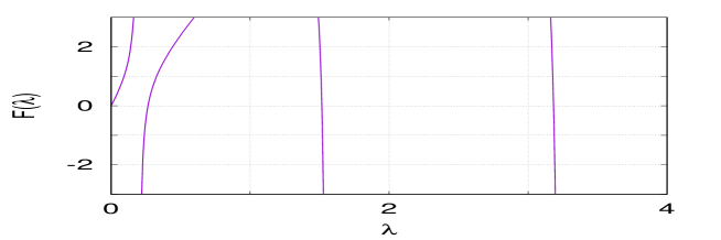
Figure 3: Plot of the function $F_{q}(\lambda)$ for $0\leq\lambda\leq 4$ showing the three chain eigenvalues for the graph $C_{4}\oplus K_{6}$.

The eigenvalues are the zeros of the function $F_{q}(\lambda)$ whose graph is presented in Fig. 3. Once these zeros are estimated, relation (3.15) allows to compute the ratio of the eigenvector components at the edge and inside the clique. The results are summarized in Table 3 for the graph $C_{4}\oplus K_{6}$ presented in section 2.2.

$n$	zero of $F_{q}(\lambda)$	$\lambda_{n}$	$C_{0}={1\over 1-\lambda_{n}}$	$v_{5}^{n}/v_{4}^{n}$
8	0.265033	0.26503	1.360	1.361
7	1.51622	1.5163	-1.9365	-1.9368
6	3.1832	3.1832	-0.4580	-0.4580

Table 3: Comparison of the zeros of the function $F_{q}(\lambda)$ and the chain eigenvalues $\lambda_{n}$ for the graph $C_{4}\oplus K_{6}$ presented in section 2.2. The ratio of the eigenvectors components at the edge and inside the clique are given in the last two columns.

As can be seen, the agreement between the eigenvalues and the zeros of $F_{q}(\lambda)$ is excellent. The ratios of the eigenvectors at the edge and inside the clique also agree well with the ones of section 2.2. Without normalization, the eigenvector components $v_{k}^{n}$ in the chain section would be

$$v_{k}^{n}=A_{n}\cos\left[\lambda_{n}(k-5)\right]+B_{n}\sin\left[\lambda_{n}(k-5)\right],$$

with $A_{n},B_{n}$ chosen as to satisfy the boundary condition at the end of the chain.

3.7 Spectrum of $K_{p}\oplus C_{q}$

We have the following theorem summarizing the spectrum of the Laplacian of $K_{p}\oplus C_{q}$.

Proposition 3.11

Let $L$ be the Laplacian of the graph $K_{p}\oplus C_{q}$, $p\geq 3$. Then the spectrum of $L$ consists of the eigenvalue $p$, of multiplicity $p-2$, a simple eigenvalue $\lambda\in(p,p+2]$, and $q$ eigenvalues in the interval $[0,4]$ (that include the simple $0$ eigenvalue).

4 Two chains connected to a clique

We now consider graphs denoted by $G=C_{q_{1}}\oplus K_{p}\oplus C_{q_{2}}$, with $p\geq 3$, $q_{1}$, $q_{2}\geq 2$ positive integers, defined by the vertex set

$${\cal V}={\cal V}_{q_{1},-}\cup{\cal V}_{p,-}\cup{\cal V}_{q_{2},+},\quad{\cal V}_{q_{1},-}=\{-q_{1}-p+2,-q_{2}-p+3,\ldots,-p-1,-p\},$$ (4.1)

with ${\cal V}_{p,-}$, ${\cal V}_{q_{1},+}$ as in (2.2), and a connectivity matrix $c$ that satisfies

$$c_{i,j}=-1,\quad\forall i,j\in{\cal V}_{p,-},$$ (4.2)

$$c_{-p,-p+1}=c_{-p+1,-p}=c_{0,1}=c_{1,0}=-1,$$ (4.3)

$$c_{i,j}=-1,\quad\forall i,j\in{\cal V}_{q_{1},-}\cup{\cal V}_{q_{2},+}\quad\hbox{with}\quad|i-j|=1,$$ (4.4)

and $c_{i,j}=0$ for all other pairs $(i,j)\in{\cal V}\times{\cal V}$. We now have a complete graph of $p$ nodes, the set ${\cal V}_{p,-}$, joined to two chains of $q_{1}-1$, $q_{2}-1$ nodes by (4.3).

Lemma 4.1

Let $L$ be the graph Laplacian of the graph $C_{q_{1}}\oplus K_{p}\oplus C_{q_{2}}$, $p\geq 6$, $q_{1}$, $q_{2}\geq 4$. Then $\lambda_{1}(L)$, $\lambda_{2}(L)\in[p,p+2]$, and $\lambda_{j}(L)=p$, $\forall j\in\{3,\ldots,p-1\}$. Also, $\lambda_{p}(L)$, $\lambda_{p+1}(L)\in(0,\hbox{min}\{\lambda_{1}(L_{C_{q}})+2,p\})$ ($\subset(0,p)$ if $p\geq 6$), $q=\hbox{max}\{q_{1},q_{2}\}$, and $\lambda_{j}(L)\in[0,4)$, $\forall j\in\{p+3,\ldots,p+q_{1}+q_{2}-2\}$.

Proof. We will apply the Weyl inequalities (3.2) using the decomposition $L=A+B$, where $A$ is the $(p+q_{1}+q_{2}-2)\times(p+q_{1}+q_{2}-2)$ block diagonal matrix with blocks $L_{C_{q_{1}}}$, $L_{K_{p}}$, and $L_{C_{q_{2}}}$. Then the only non-vanishing elements of $B$ are $B(q_{1}-1,q_{1}-1)=B(q_{1},q_{1})=B(q_{1}+p-1,q_{1}+p-1)=B(q_{1}+p,q_{1}+p)=1$, and $B(q_{1},q_{1}-1)=B(q_{1}-1,q_{1})=B(q_{1}+p,q_{1}+p-1)=B(q_{1}+p-1,q_{1}+p)=-1$.

We then have $\lambda_{j}(A)=p$ if $j\in\{1,\ldots,p\}$, and $\lambda_{p-1+k}(A)=\in(0,4)$ for $k\in\{1,q_{1}+q_{1}-4\}$. Also $\lambda_{p+q_{1}+q_{2}-4}(A)=\lambda_{p+q_{1}+q_{2}-3}(A)=\lambda_{p+q_{1}+q_{2}-2}(A)=0$. Furthermore, $\lambda_{1}(B)=\lambda_{2}(B)=2$, and $\lambda_{j}(B)=0$, $\forall j\in\{3,\ldots,p+q_{1}+q_{2}-2\}$.

We use $\lambda_{j}(A)\leq\lambda_{j}(A+B)$, $j=1,\ldots,p+q_{1}+q_{2}-2$, see (3.2), as lower bounds.

For the upper bounds we first have

$$\lambda_{1}(A+B)\leq\lambda_{1}(A)+\lambda_{1}(B)=p+2,$$

$$\lambda_{2}(A+B)\leq\hbox{min}\{\lambda_{2}(A)+\lambda_{1}(B),\lambda_{1}(A)+\lambda_{(}B)\}=p+2.$$

For $j\in{3,\ldots,p-1\ }$ we have

$$\lambda_{j}(A+B)\leq\hbox{min}\{\lambda_{j}(A)+\lambda_{1}(B),\lambda_{j-1}(A)+\lambda_{2}(B),\ldots,\lambda_{1}(A)\}=p,$$

using $\lambda_{j}(B)=0$, $\forall j\in\{3,\ldots,p+q_{1}+q_{2}-2\}$. Also,

$$\lambda_{p}(A+B) \leq \hbox{min}\{\lambda_{p}(A)+\lambda_{1}(B),\lambda_{p-1}(A)+\lambda_{2}(B),\ldots,\lambda_{1}(A)\}$$

$$= \hbox{min}\{\hbox{max}\{\lambda_{1}(L_{C_{q_{1}}}),\lambda_{1}(L_{C_{q_{2}}})\}+2,p\},$$

$$\lambda_{p+1}(A+B) \leq \hbox{min}\{\lambda_{p+1}(A)+\lambda_{1}(B),\lambda_{p}(A)+\lambda_{2}(B),\ldots,\lambda_{1}(A)\}$$

$$= \hbox{min}\{\hbox{max}\{\lambda_{1}(L_{C_{q_{1}}}),\lambda_{1}(L_{C_{q_{2}}})\}+2,p\}.$$

If $p\geq 6$ then $\lambda_{1}(L_{C_{q}})+2<6\leq p$, therefore $\lambda_{p}(A+B)$, $\lambda_{p+1}(A+B)<p$.

For $j\in\{p+2,\ldots,p+q_{1}+q_{2}-5\}$, i.e. $j=p-1+k$, $k\in\{3,\ldots,p+q_{1}+q_{2}-4\}$, we have

$$\lambda_{p-1+k}(A+B) \leq \hbox{min}\{\hbox{max}\{\lambda_{1}(L_{C_{q_{1}}}),\lambda_{1}(L_{C_{q_{1}}})\}+2\ldots,\lambda_{1}(A)\}$$

$$= \hbox{min}\{\hbox{max}\{\lambda_{1}(L_{C_{q_{1}}}),\lambda_{1}(L_{C_{q_{1}}})\}+2,p\},$$

Also

$$\lambda_{p+q_{1}+q_{2}-4}(A+B)\leq\min_{l=1,2}\{2,\lambda_{q_{j}-2}(L_{C_{q_{l}}})+2,\lambda_{q_{l}-3}(L_{C_{q_{l}}})\},$$

therefore $\lambda_{p+q_{1}+q_{2}-4}(A+B)<4$ if $q_{1}$, $q_{2}\geq 4$ using (2.1) for $\lambda_{q-3}(L_{C_{q}})$, $q\geq 4$, and

$$\lambda_{p+q_{1}+q_{2}-3}(A+B)\leq\min_{l=1,2}\{2,\lambda_{q_{j}-2}(L_{C_{q_{l}}})<4,$$

$\lambda_{p+q_{1}+q_{2}-2}(A+B)=0$. The statement follows by combining the above with the lower bounds. $\Box$

4.1 Clique eigenvalues

Proposition 4.2

Let $L$ be the Laplacian of the graph $C_{q_{1}}\oplus K_{p}\oplus C_{q_{2}}$, $p\geq 4$, $q_{1}$, $q_{2}\geq 2$. Then there exists a subspace $E_{K}$ of dimension $p-3$ such that $v\in E_{K}$ satisfies $Lv=pv$, and $v_{j}=0$, $\forall j\notin\{-p+2,\ldots,-1\}$.

Proof. Let $k\in\{2,\ldots,p-2\}$ and define the vectors $v^{k}\in l^{2}$ by

$$v^{k}_{-1}=1,\quad v^{k}_{-k}=-1,\quad v^{k}_{j}=0,\quad\forall j\in{\cal V}\setminus\{-1,-k\}.$$ (4.5)

The $v^{k}$ are linearly independent and the statement will follow by checking that $Lv^{k}=pv^{k}$, $\forall k\in\{2,\ldots,p-2\}$. Let $i\geq 1$ or $i\leq-(p-1)-1$. Then $(Lv^{k})_{i}=pv^{k}_{i}$, as in (3.4). The case $i\in\{-(p-1),\ldots,0\}\setminus\{-1,-k\}$ is as in (3.4). The cases $i=-1$, $-k$ follow from (3.6), (3.7) respectively. $\Box$

As for the chain connected to a clique, the result extends to the case of two infinite chains $q_{1}$, $q_{2}=\infty$.

Proposition 4.3

Let $L$ be the Laplacian of the graph $C_{\infty}\oplus K_{p}\oplus C_{\infty}$, $p\geq 4$. Then there exists a subspace $E_{K}\in l^{2}$ of dimension $p-3$ such that $v\in E_{K}$ satisfies $Lv=pv$, and $v_{j}=0$, $\forall j\notin\{-p+2,\ldots,-1\}$.

4.2 Edge eigenvalues

Let $v\in l^{2}$ be an eigenvector of $L$ for the graph $C_{q}\oplus K_{p}\oplus C_{q}$, $q\geq 2$ (including the case $q=\infty$). Then $v$ is symmetric if $v_{-p-1-n}=v_{n}$, for all integer $n\geq 0$, and antisymmetric if $v_{-p-1-n}=-v_{n}$, for all integer $n\geq 0$.

Proposition 4.4

Let $L$ be the Laplacian of the graph $C_{\infty}\oplus K_{p}\oplus C_{\infty}$, $p\geq 5$, and let $E_{K}$ be as in Proposition 4.2. Then all eigenvectors $v\in l^{2}\cap E_{K}^{\perp}$ of $L$ corresponding to eigenvalues $\lambda>4$ are either symmetric or antisymmetric. $\lambda>4$ is the eigenvalue of a symmetric eigenvector $v^{S}\in l^{2}\cap E_{K}^{\perp}$ of $L$ if and only if $F_{S}(\lambda)=0$, where

$$F_{S}(\lambda)=(-\lambda+2)\sigma_{+}-(-\lambda+p-1)(-\lambda+2)+2(p-2).$$ (4.6)

$\lambda>4$ is the eigenvalue of a symmetric eigenvector $v^{A}\in l^{2}\cap E_{K}^{\perp}$ of $L$ if and only if $F_{A}(\lambda)=0$, with

$$F_{A}(\lambda)=\sigma_{+}-(-\lambda+p+1).$$ (4.7)

$\sigma_{+}=\sigma_{+}(\lambda)$ in (4.6), (4.7) is as in (3.11), Furthermore, both equations $F_{A}=0$, $F_{S}=0$ have exactly one solution in $(p,p+2)$ and no solutions in $(4,p]\cup[p+2,+\infty)$.

Proof. We construct $v\in l^{2}$ that satisfy $Lv=\lambda v$, with $\lambda>4$. We first let $v$ be orthogonal to the span of the $p-3$ eigenvectors of Proposition 3.4 , or

$$-v_{-p+2}+v_{-1}=0,\quad\ldots-v_{-2}+v_{-1}=0,$$

therefore

$$v_{-p+2}=\ldots=v_{-1}=C_{0}$$ (4.8)

for some real $C_{0}$. We also let

$$C_{1}=v_{0},\quad C_{-1}=v_{-p+1}.$$ (4.9)

The condition $Lv=\lambda v$ at the nodes $k=-p+2,\ldots,-1$ leads to

$$(p-3)C_{0}+C_{1}+C_{-1}-(p-1)C_{0}=-\lambda C_{0},$$ (4.10)

for all $k=-p+2,\ldots,-1$, or

$$C_{1}+C_{-1}=(-\lambda+2)C_{0}.$$ (4.11)

Let

$$C_{2}=v_{1},\quad c_{-2}=v_{-p}.$$ (4.12)

Then $Lv=\lambda v$ at $k=0$ is

$$-\sum_{j=-p+1}^{-1}c_{0,j}v_{j}+d_{0}v_{0}-v_{1}=\lambda v_{0},$$

and reduces to

$$C_{-1}+(p-2)C_{0}+C_{2}=(-\lambda+p)C_{1}.$$ (4.13)

Similarly, $Lv=\lambda v$ at $k=-p+1$ is

$$-\sum_{j=-p+1}^{-1}c_{-p+1,j}v_{j}+d_{-p+1}v_{-p+1}-v_{-p}=\lambda v_{-p+1},$$

and reduces to

$$C_{1}+(p-2)C_{0}+C_{-2}=(-\lambda+p)C_{-1}.$$ (4.14)

Considering $Lv=\lambda v$ at the nodes $j\geq 1$, we argue as in the proof of Proposition 3.6 to obtain

$$C_{2}=\sigma_{+}C_{1}.$$ (4.15)

On the other hand, $Lv=\lambda v$ at the nodes $j\geq-p$ is

$$-v_{j-1}+2v_{j}-v_{j+1}=\lambda v_{j},\quad\forall j\leq-p.$$ (4.16)

Letting

$$z_{j}=\begin{pmatrix}v_{j}\\ v_{j+1}\end{pmatrix},~{}~{}j\geq-p,$$

(4.16) is equivalent to

$$z_{j+1}=M_{\lambda}z_{j},\quad\forall j\leq-p-1,$$ (4.17)

with $M_{\lambda}$ as in (3.9), or

$$z_{-p-n}=(M_{\lambda}^{-1})^{n}z_{p},\quad\forall n\geq 0,$$ (4.18)

therefore if $z_{-p}=av^{+}+bv^{-}$, $a$, $b$ real, we have

$$z_{-p-n}=a\sigma_{+}^{-n}v^{+}+b\sigma_{-}^{-n}v^{-}=a\sigma_{-}^{n}v^{+}+b\sigma_{+}^{n}v^{-},\quad\forall,n\geq 0$$ (4.19)

by $\sigma_{-}\sigma_{+}=1$. By $\lambda>4$, $|\sigma_{-}|>1$, the condition $v\in l^{2}$ leads to $a=0$. We must then require

$$z_{-p}=\begin{pmatrix}v_{-p}\\ v_{-p+1}\end{pmatrix}=b\begin{pmatrix}1\\ \sigma_{-}\end{pmatrix}$$

for some real $b$, or equivalently

$$C_{-2}=\sigma_{+}C_{-1}$$ (4.20)

by (4.9), (4.12).

The possible eigenvectors $v\in l^{2}\cap{E_{K}}^{\perp}$ of $L$ are determined by equations (4.11), (4.13), (4.14), (4.15), (4.20) for the $C_{-2},\ldots,C_{2}$. We claim that there are only two nontrivial solutions, corresponding to $C_{-1}=C_{1}$ and $C_{-1}=-C_{1}$, leading to symmetric and antisymmetric eigenvectors respectively.

To show the claim, we first use (4.15), (4.20) to reduce the system to three equations for $C_{-1}$, $C_{0}$, $C_{1}$. We then add and subtract (4.13), (4.14), to obtain

$$(C_{-1}+C_{1})(-\lambda+p-\sigma_{+}-1)=2(p-2)C_{0},$$ (4.21)

and

$$(C_{-1}-C_{1})(-1+\sigma_{+}+\lambda-p)=0.$$ (4.22)

By (4.22) we either have $C_{-1}=C_{1}$, the symmetric case, or

$$\sigma_{+}=-\lambda+p+1,$$ (4.23)

which by (4.21) implies

$$-(C_{-1}+C_{1})=(p-2)C_{0}.$$ (4.24)

Suppose that $C_{0}\neq 0$, then (4.24), (4.11) imply $\lambda=p$. Then (4.23) implies $\sigma_{+}=1$, but this contradicts $\sigma_{+}\in(-1,0)$, from (3.11) with $\lambda>4$. It follows that $C_{0}=0$. By (4.23) we then have $C_{-1}=-C_{1}$, the antisymmetric case.

To see that the corresponding eigenvalues belong to $(p,p+2)$ we first consider the antisymmetric case $C_{-1}+C_{1}=0$. The eigenvalue $\lambda$ then satisfies (4.23), with $\sigma_{+}$ as in (3.11). Let

$$F_{A}(\lambda)=\sigma_{+}-(-\lambda+p+1).$$ (4.25)

$F_{A}$ is continuous and $F_{A}(p)=\sigma_{+}-1<0$ by $\sigma_{+}\in(-1,0)$. Also, $F_{A}(p+2)=\sigma_{+}+1>0$ by $\sigma_{+}\in(-1,0)$. Therefore we have at least one antisymmetric eigenvector with eigenvalue $\lambda\in(p,p+2)$.

We check that $F_{A}^{\prime}(\lambda)>0$ for $\lambda\in(p,p+2)$. Let $x=-\lambda+2$, and examine ${\tilde{F}}(x)=F(\lambda(x))$ for $x\in(-p,-p+2)$. We have

$${\tilde{F}}^{\prime}_{A}(x)={\tilde{\sigma}}^{\prime}(x)-1<0.$$

We saw in the proof of Proposition 3.6 that ${\tilde{\sigma}}^{\prime}(x)<-1/2$, for all $x\in(-p,-p+2)$, therefore $F_{A}^{\prime}(\lambda)=-{\tilde{F}}_{A}^{\prime}(x)>0$, for all $\lambda\in(p,p+2)$.

Also, $\lambda\leq p$ would imply $\sigma_{+}\geq 1$ by (4.23), contradicting $\sigma_{+}\in(-1,0)$. Similarly, $\lambda\geq p+2$ and (4.23) would imply $\sigma_{+}\leq-1$, a contradiction.

We conclude that equation (4.23) for antisymmetric eigenvectors has exactly one solution in $(p,p+2)$ and no other solution satisfying $\lambda>4$.

In the symmetric case $C_{-1}=C_{1}$, by (4.11) we must also have $C_{0}\neq 0$, otherwise we have a trivial solution. Combining (4.21) and (4.11), the corresponding eigenvalue $\lambda$ must then satisfy

$$(-\lambda+2)(-\lambda+p-\sigma_{+}-1)=2(p-2),$$ (4.26)

or equivalently

$$\sigma_{+}=-\lambda+p-1-2\frac{p-2}{-\lambda+2}.$$ (4.27)

Let

$$F_{S}(\lambda)=(-\lambda+2)\sigma_{+}-(-\lambda+p-1)(-\lambda+2)+2(p-2),$$ (4.28)

with with $\sigma_{+}$ as in (3.11). $F_{S}$ is continuous and we have

$$F_{S}(p)=(p-2)(2-\sigma_{+})>0$$

by $\sigma_{+}\in(-1,0)$. Also,

$$F_{S}(p+2)=-p(1+\sigma_{+})-4<0$$

by $\sigma_{+}\in(-1,0)$. There then at least one symmetric eigenvector with eigenvalue $\lambda\in(p,p+2)$.

We see that $F_{S}^{\prime}(\lambda)<0$ for $\lambda\in(p,p+2)$. Let $x=-\lambda+2$, and examine ${\tilde{F}}(x)=F(\lambda(x))$ for $x\in(-p,-p+2)$. We have

$${\tilde{F}}_{S}^{\prime}(x)={\tilde{\sigma}}_{+}(x)+x{\tilde{\sigma}}^{\prime}_{+}(x)-2x-p+3.$$

By $x<-p+2$ we have $-2x>2p-4$, therefore

$${\tilde{F}}_{S}^{\prime}(x)>x{\tilde{\sigma}}^{\prime}_{+}(x)+p-1+{\tilde{\sigma}}_{+}(x).$$

We saw in the proof of Proposition 3.6 that ${\tilde{\sigma}}^{\prime}(x)<-1/2$, for all $x\in(-p,-p+2)$, therefore $x{\tilde{\sigma}}^{\prime}_{+}(x)>0$, $\forall x\in(-p,-p+2)$. Also $p-1+{\tilde{\sigma}}_{+}>p-2>0$. Thus $F_{S}^{\prime}(\lambda)=-{\tilde{F}}_{S}^{\prime}(x)<0$, for all $\lambda\in(p,p+2)$.

Also, suppose that $\lambda\leq p$, then $-(-\lambda+2)\leq p-2$ and 4.27 would imply

$$\sigma_{+}\geq-1+2\frac{p-2}{\lambda-2}\geq 1,$$

contradicting $\sigma_{+}\in(-1,0)$. Similarly, $\lambda\geq p+2$ and 4.27 imply

$$\sigma_{+}\leq-3-2\frac{p-2}{-\lambda+2}\leq-3+2\frac{p-2}{p}\leq-1,$$

contradicting $\sigma_{+}\in(-1,0)$.

Thus equation (4.26) for symmetric eigenvectors has exactly one solution in $(p,p+2)$ and no other solution satisfying $\lambda>4$.

$\Box$

Remark 4.5

The eigenvalue corresponding to the antisymmetric eigenvector is larger than the one for the symmetric eigenvector. In section 4.4 we derive the asymptotic estimates (4.32,4.33) of these eigenvalues for large $p$.

Proposition 4.6

Let $L$ be the Laplacian of $C_{\infty}\oplus K_{p}\oplus C_{\infty}$, $p\geq 6$. Then $\sigma_{e}({L})=[0,4]$.

The proof uses the argument of Proposition 3.7.

As for $K_{p}\oplus C_{\infty}$, we have the following theorem for the spectrum of $C_{\infty}\oplus K_{p}\oplus C_{\infty}$, $p\geq 6$.

Proposition 4.7

Let $L$ be the Laplacian of the graph $C_{\infty}\cup K_{p}\cup C_{\infty}$, $p\geq 6$. Then the spectrum of $L$ is a union of the disjoint sets $[0,4]$ (the essential spectrum of $L$), and $\{\lambda_{1},\lambda_{2},p\}$, with $\lambda_{1}\geq\lambda_{2}\in(p,p+2)$ (the point spectrum of $L$).

Remark 4.8

By Proposition 4.3, for $p=4$ we have three clique eigenvalues $\lambda=4\in\sigma_{e}(L)$.

4.3 Edge eigenvectors for $C_{q_{1}}\oplus K_{p}\oplus C_{q_{2}}$

We have the following proposition showing the existence of two edge eigenvectors for the graph $C_{q_{1}}\oplus K_{p}\oplus C_{q_{2}}$.

Proposition 4.9

Let $L$ be the Laplacian of the graph $C_{q_{1}}\oplus K_{p}\oplus C_{q_{2}}$, $p\geq 6$, $q_{1}$, $q_{2}\geq 3$. Then $\lambda>4$ is an eigenvalue of $L$ with corresponding eigenvector $v\in E_{K}^{\perp}$ if and only if $D_{q_{1},p,q_{2}}(\lambda)=0$, where

$$D_{q_{1},p,q_{2}}(\lambda)=(p-2)(2-Q_{q_{1}}-Q_{q_{2}})-(-\lambda+2)(Q_{q_{1}}Q_{q_{2}}-1),$$ (4.29)

where

$$Q_{q}=\sigma_{+}\frac{1+\sigma_{+}^{2q-3}}{1+\sigma_{+}^{2q-1}}-(-\lambda+p),$$ (4.30)

and $\sigma_{+}=\sigma_{+}(\lambda)$ is as in (3.11). $D_{q_{1},p,q_{2}}(\lambda)=0$ has exactly two solutions in $(p,p+2]$ and no solutions in $(4,p]\cup(p+2,+\infty)$. In the case $q_{1}=q_{2}=q$, we have the factorization $D_{q_{1},p,q_{2}}(\lambda)=-F_{A,q}(\lambda)F_{S,q}(\lambda)$ with

$$F_{S,q}(\lambda)=(-\lambda+2)(Q_{q}+1)+2(p-2),\quad F_{A,q}(\lambda)=1-Q_{q}.$$ (4.31)

Solutions of $F_{S,q}(\lambda)=0$, $F_{A,q}(\lambda)=0$ correspond to symmetric and antisymmetric eigenvectors of $L$ respectively. Furthermore, both equations $F_{A,q}(\lambda)=0$, $F_{S,q}(\lambda)=0$, $q\geq 3$, have exactly one solution in $(p,p+2)$ and no solutions in $(4,p]\cup[p+2,+\infty)$.

The proof combines the arguments of Propositions 4.4, 3.10 and is given in the appendix

We have the following theorem for the whole spectrum of the graph $C_{q_{1}}\oplus K_{p}\oplus C_{q_{2}}$.

Proposition 4.10

Let $L$ be the Laplacian of the graph $C_{q_{1}}\oplus K_{p}\oplus C_{q_{2}}$, $p\geq 6$, $q_{1}$, $q_{2}\geq 2$. Then the spectrum of $L$ consists of the eigenvalue $p$, of multiplicity $p-3$, two eigenvalues $\lambda_{1}$, $\lambda_{2}\in(p,p+2]$. All other eigenvalues are in the interval $[0,4]$

4.4 Numerical calculations and asymptotic estimates for large $p$

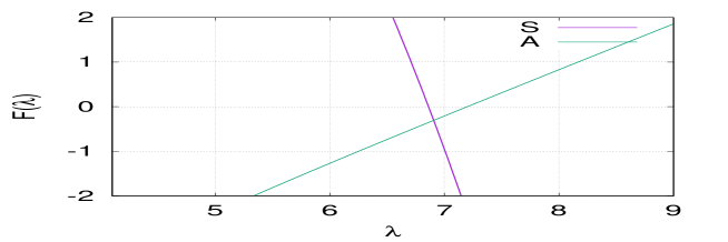
Figure 4: Plot of the functions $F_{S}(\lambda)$ and $F_{A}(\lambda)$ for the graph $C_{\infty}\oplus K_{6}\oplus C_{\infty}$.

We now consider the asymptotic behavior of $\lambda$ in the antisymmetric and symmetric cases. For that we will use the asymptotic estimates of $\sigma_{+}$ (3.26)

$$\sigma_{+}\approx{1\over 2-\lambda}$$

First, assume an antisymmetric solution so that $C_{0}=0$ Then,

$$F_{A}(\lambda)=\sigma_{+}-(-\lambda+p+1)a=0$$

From this equation, we get

$${1\over 2-\lambda}=-\lambda+p+1$$

which yields the following second degree equation for $\lambda$

$$\lambda^{2}-\lambda(p+3)+2(p+1)-1=0.$$

The interesting solution is

$$\lambda={p+3\over 2}+{1\over 2}\sqrt{(p+3)^{2}-4(2p+1)}$$

Expanding the square root, we obtain the final estimate

$$\lambda=p+1+{1\over p},$$ (4.32)

which yields $\lambda=7.16$ for $p=6$ close to the numerical value. The quantity $\sigma_{+}$ is

$$\sigma_{+}={p\over p(1-p)-1}.$$

For $p=6$, we have $\sigma_{+}=-0.19$.

For the symmetric case, we have

$$F_{S}(\lambda)=(-\lambda+2)\sigma_{+}-(-\lambda+p-1)(-\lambda+2)+2(p-2)=0$$

Substituting equation (3.26) in $F_{S}(\lambda)=0$ yields the following second degree equation for $\lambda$

$$\lambda^{2}-\lambda(p+1)+2=0.$$

The interesting root is

$$\lambda={p+1\over 2}+{1\over 2}\sqrt{(p+1)^{2}-8}.$$

Expanding the square root as above yields the estimate

$$\lambda=p+1-{2\over p+1}.$$ (4.33)

For $p=6$, we obtain $\lambda=6.71$.

5 Graphs of complete graphs: results and conjectures

To conclude the article we present two conjectures on the spectrum of graphs composed of complete graphs $K_{p}$ connected by chains.

We introduce a graph of complete graphs with the following.

Definition 5.1

A graph of complete graphs is the set ${\cal G}=\{\tilde{V},\tilde{E}\}$ where $\tilde{V}=\{K_{p_{1}},K_{p_{2}},\dots,K_{p_{N}}\}$ where $K_{p_{i}}$ is a $p_{i}$ complete graph. The edges are chains connecting the vertices $K_{p_{i}}$.

An example of such a graph of complete graphs is shown in Fig. 5.

Figure 5: A graph of 5 complete graphs connected by chains

Assume $p_{i}\geq 5$ and the length of the edges (chains) greater than 3 and denote $d_{i}$ the degree of $K_{p_{i}}$ in ${\cal G}$. We have the following result.

Proposition 5.2

For a graph of complete graphs ${\cal G}$ there are at most $p_{i}-d_{i}-2$ clique eigenvalues $p_{i}$ for $i\in\{1,\dots,N\}$. There is exactly $p_{i}-d_{i}-2$ clique eigenvalues if $K_{p_{i}}$ is connected to edges at different vertices.

The proof is an immediate generalization of the results on the clique eigenvalues obtained in sections 3 and 4.

We also give the following conjecture.

Proposition 5.3

For a graph of complete graphs ${\cal G}$ there are $d_{i},~{}i\in\{1,\dots,N\}$ edge eigenvectors with eigenvalues in $]p_{i},p_{i}+2[$ .

As a numerical example, we show a graph ${\cal G}$ composed of $K_{10}$ and three chains.

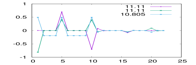
Figure 6: Plot of the three edge eigenvectors for the graph $G=K_{10}\oplus C^{1}\oplus C^{2}\oplus C^{3}$. The clique is $K_{10}=\{1,2,\dots,10\}$ and the chains are $C^{1}=\{20,21,22\}$, $C^{2}=\{16,17,18,19\}$ and $C^{3}=\{11,12,13,14,15\}$ connected at vertices $1$, $5$ and $10$ respectively.

There are $N$ edge eigenvectors of eigenvalue $\lambda>p$. One of them is symmetric, and $N-1$ are antisymmetric. For the antisymmetric edge eigenvector, the eigenvalue is the one calculated for the graph with a clique and two chains. For example for the $G=K_{10}\oplus C^{1}\oplus C^{2}\oplus C^{3}$ we have $\lambda=11.11$ for the antisymmetric eigenvector. Both symmetric and antisymmetric eigenvectors can be labeled using a three component vector with $\pm 1$, each component corresponding to a chain connected to $=K_{10}$. Using this shorthand notation, the symmetric and antisymmetric eigenvectors are

$$s=\begin{pmatrix}1\cr 1\cr 1\end{pmatrix},~{}~{}a^{1}=\begin{pmatrix}0\cr 1\cr-1\end{pmatrix},~{}~{}a^{2}=\begin{pmatrix}1\cr 0\cr-1\end{pmatrix},$$

where the antisymmetric eigenvectors correspond to the eigenvalue of multiplicity $N-1=2$. These eigenvectors are shown in Fig. 6.

Acknowledgments. We acknowledge the support of a french-mexican Ecos-Conacyt grant. JGC thanks IIMAS for financial support and was partially funded by ANR grant ”Fractal grid”. PP thanks Papit IN112119 for partial support.

6 Appendix: proof of existence of edge eigenvector for $C_{q_{1}}\oplus K_{p}\oplus C_{q_{2}}$

Proof. To construct $v$ that satisfies $Lv=\lambda v$, $\lambda>4$ and is orthogonal to the span of the $p-3$ eigenvectors of Proposition 4.2 we argue as in the proof of Proposition 4.2. Considering $Lv=\lambda v$ at the sites $j=-p+1,\ldots,0$, and letting $C_{-2}=v_{-p}$, $C_{-1}=v_{-p+1}$, $C_{0}=v_{-p+2}=\ldots=v_{-1}$, $C_{1}=v_{0}$, and $C_{2}=v_{1}$ we obtain the equations

$$C_{1}+C_{-1}=(-\lambda+2)C_{0},$$ (6.1)

$$C_{-1}+(p-2)C_{0}+C_{2}=(-\lambda+p)C_{1},$$ (6.2)

$$C_{1}+(p-2)C_{0}+C_{-2}=(-\lambda+p)C_{-1},$$ (6.3)

i.e. as in (4.11), (4.13), (4.14).

We will express $C_{2}$, $C_{-2}$ in terms of the $C_{1}$, $C_{-1}$ respectively by analyzing the $Lv=\lambda v$ at the remaining sites.

Consider first $Lv=\lambda v$ at the nodes $1\leq j\leq q_{2}-2$,

$$-v_{j-1}+2v_{j}-v_{j+1}=\lambda v_{j},\quad\forall j\in\{1,\ldots,q_{2}-2\}.$$ (6.4)

We argue as in the proof of Proposition 3.10. Letting $z_{j}=(v_{j},v_{j+1})^{T}$, $0\leq j\leq q_{2}-1$, (6.13) is equivalent to

$$z_{j+1}=M_{\lambda}z_{j},\quad\forall j\in\{1,\ldots,q_{2}-2\},$$ (6.5)

with $M_{\lambda}$ as in (3.9). Then $z_{0}=a_{2}v^{+}+b_{2}v^{-}$, $a_{2}$, $b_{2}$ real, implies

$$z_{n}=a_{2}\sigma_{+}^{n}v^{+}+b_{2}\sigma_{-}^{n}v^{-},\quad\forall n\in\{0,\ldots,q_{2}-2\}.$$ (6.6)

Evaluating at $n=q_{2}-2$ and comparing to $Lv=\lambda v$ at the node $n=q_{2}-1$, namely

$$v_{q_{2}-1}=\frac{v_{q_{2}-2}}{-\lambda+1},$$ (6.7)

we arrive at

$$\frac{1}{-\lambda+1}[a_{2}\sigma_{+}^{q_{2}-2}+b_{2}\sigma_{-}^{q_{2}-2}]=a_{2}\sigma_{+}^{q_{2}-1}+b_{2}\sigma_{-}^{q_{2}-1}.$$ (6.8)

Arguing as in as in the proof of Proposition 3.10 we have

$$\frac{b_{2}}{a_{2}}=\sigma_{+}^{2q_{2}},$$ (6.9)

and $a_{2}b_{2}\neq 0$. Comparing expressions for $v_{0}$, $v_{1}$, and $z_{0}=a_{2}v^{+}+b_{2}v^{-}$, using also (6.9) for the ratio $b_{2}/a_{2}$, we must require

$$\left[\begin{array}[]{c}C_{1}\\ C_{2}\end{array}\right]=a_{2}\left(\left[\begin{array}[]{c}1\\ \sigma_{+}\end{array}\right]+\sigma_{+}^{2q_{2}-1}\left[\begin{array}[]{c}1\\ \sigma_{-}\end{array}\right]\right).$$ (6.10)

Then

$$C_{1}=a_{2}(1+\sigma_{+}^{2q_{2}-1}),\quad C_{2}=a_{2}(\sigma_{+}+\sigma_{+}^{2q_{2}-2}),$$ (6.11)

and therefore

$$C_{2}=C_{1}\sigma_{+}\frac{1+\sigma_{+}^{2q_{2}-3}}{1+\sigma_{+}^{2q_{2}-1}}.$$ (6.12)

Consider now $Lv=\lambda v$ at the nodes $-p-q_{1}+3\leq j\leq-p$,

$$-v_{j-1}+2v_{j}-v_{j+1}=\lambda v_{j},\quad\forall j\in\{-p-q_{1}+3,\ldots,-p\}.$$ (6.13)

Letting $z_{j}=[v_{j},v_{j+1}]^{T}$, $-p-q_{1}+2\leq j\leq-p-1$, (6.13) is equivalent to

$$z_{j+1}=M_{\lambda}z_{j},\quad\forall j\in\{-p-q_{1}+2,\ldots,-p-1\}.$$ (6.14)

Then $z_{-p-q_{1}+2+n}=M_{\lambda}^{n}z_{-p-q_{1}+2}$, $n\in\{0,\ldots,\tilde{q}_{1}-2\}$ and for $n=q_{1}-2$ we have

$$z_{-p}=M_{\lambda}^{q_{1}-2}z_{-p-q_{1}+2}.$$ (6.15)

Setting $z_{-p}=a_{1}v^{+}+b_{1}v^{-}$, we then have

$$z_{-p-q_{1}+2}=(M^{-1}_{\lambda})^{q_{1}-2}z_{-p}=a_{1}\sigma_{-}^{q_{1}-2}v^{+}+b_{1}\sigma_{+}^{q_{1}-2}v^{-}.$$ (6.16)

Therefore

$$\left[\begin{array}[]{c}v_{-p-q_{1}+2}\\ v_{-p-q_{1}+3}\end{array}\right]=\left[\begin{array}[]{c}a_{1}\sigma_{-}^{q_{1}-2}+b_{1}\sigma_{+}^{q_{1}-2}\\ a_{1}\sigma_{-}^{q_{1}-3}+b_{1}\sigma_{-}^{q_{1}-3}\end{array}\right].$$ (6.17)

At the same time, $Lv=\lambda v$ at the node $-p-q_{1}+2$ yields

$$v_{-p-q_{1}+2}=\frac{v_{-p-q_{1}+3}}{-\lambda+1}.$$ (6.18)

Comparing (6.17), (6.18) we must have

$$\frac{1}{-\lambda+1}[a_{1}\sigma_{+}^{q_{1}-3}+b_{1}\sigma_{-}^{q_{1}-3}]=a_{1}\sigma_{+}^{q_{1}-2}+b_{1}\sigma_{-}^{q_{1}-2}.$$ (6.19)

Note that this is (3.39) in the proof of Proposition 3.10 with $q=q_{1}-1$, $a=a_{1}$, $b=b_{1}$, and $\sigma\pm=\sigma_{\mp}$. Arguing similarly we have

$$\frac{a_{1}}{b_{2}}=\sigma_{+}^{2q_{1}-3}.$$ (6.20)

Comparing expressions for $v_{-p}=C_{-2}$, $v_{-p+1}=C_{-1}$, and $z_{-p}=a_{1}v^{+}+b_{2}v^{-}$, using also (6.20) for the ratio $a_{1}/b_{2}$ we must require

$$\left[\begin{array}[]{c}C_{-2}\\ C_{-1}\end{array}\right]=b_{1}\left(\sigma_{+}^{2q_{1}-3}\left[\begin{array}[]{c}1\\ \sigma_{+}\end{array}\right]+\left[\begin{array}[]{c}1\\ \sigma_{-}\end{array}\right]\right).$$ (6.21)

Then

$$C_{-2}=b_{1}(\sigma_{+}^{2q_{1}-3}+1),\quad C_{-1}=b_{1}(\sigma_{+}^{2q_{1}-2}+\sigma_{-}),$$ (6.22)

and

$$C_{-2}=C_{-1}\sigma_{+}\frac{1+\sigma_{+}^{2q_{1}-3}}{1+\sigma_{+}^{2q_{1}-1}}.$$ (6.23)

By (6.12), (6.23), system (6.1), (6.2), (6.3) is reduced to

$$C_{1}+C_{-1}-(-\lambda+2)C_{0} = 0,$$ (6.24)

$$Q_{q_{2}}C_{1}+C_{-1}+(p-2)C_{0} = 0,$$ (6.25)

$$C_{1}+Q_{q_{1}}C_{-1}+(p-2)C_{0} = 0,$$ (6.26)

with $Q_{q}$ as in (4.30). This is a homogeneous system of the form $Mx=0$, with $x=[C_{-1},C_{1},C_{0}]$, $M$ defined implicitly by (6.24)-(6.26).

We compute that $\hbox{det}M=D_{q_{1},p,q_{2}}(\lambda)$, with $D_{q_{1},p,q_{2}}(\lambda)$ given by (4.29). We then have the first statement of the proposition, since the trivial solution of would lead to a trivial solution of $Lv=\lambda v$.

We now examine $D_{q_{1},p,q_{2}}(\lambda)=0$ with $\lambda>4$. We first show that there are no solutions in $(4,p]$. By (4.29) $D_{q_{1},p,q_{2}}(\lambda)=0$ is equivalent to

$$(p-2)(2-Q_{q_{1}}-Q_{q_{2}})=(\lambda-2)(1-Q_{q_{1}}Q_{q_{2}}).$$ (6.27)

By $\lambda>4$, we have $\sigma_{+}\in(-1,0)$, and $G_{q}=(1+\sigma_{+}^{2{\tilde{q}}-1})(1+\sigma_{+}^{2{\tilde{q}}+1})^{-1}\in(0,1)$. By definition (4.30) we then have $Q_{q}\in(-1,0)$; Assume $\lambda\in(4,p]$, then the right hand side of (6.27) satisfies

$$(p-2)(2-Q_{q_{1}}-Q_{q_{2}})>2(p-2)(p-\lambda+1)\geq 2(p-2).$$ (6.28)

Considering the left hand side of (6.27), we have

$$1-Q_{q_{1}}Q_{q_{2}}\leq 1$$ (6.29)

since

$$Q_{q_{1}}Q_{q_{2}}=\sigma_{+}^{2}G_{q_{1}}G_{q_{2}}+(p-\lambda)(-\sigma_{+}G_{q_{1}}-\sigma_{+}G_{q_{2}}+p-\lambda)>0.$$

If $1-Q_{q_{1}}Q_{q_{2}}\leq 0$, then the left hand side of (6.27) is nonpositive, and by (6.28), equality (6.27) can not be satisfied. If $1-Q_{q_{1}}Q_{q_{2}}>0$, then the assumption $\lambda\in(4,p]$, and (6.29) imply

$$(\lambda-2)(1-Q_{q_{1}}Q_{q_{2}})\leq p-2.$$

By $p>2$ and (6.28) we see that again (6.27) can not be satisfied.

Combining with assumption $p\geq 6$ and Proposition 4.1, all solutions of $D_{q_{1},p,q_{2}}(\lambda)=0$ with $\lambda>4$ must belong to the interval $(p,p+2]$. moreover $D_{q_{1},p,q_{2}}(\lambda)=0$ has exactly two solutions in $(p,p+2]$.

We now consider the case $q_{1}=q_{2}=q$ we have the factorization $D_{q_{1},p,q_{2}}(\lambda)=-F_{A,q}(\lambda)F_{S,q}(\lambda)$.

We first check that $F_{S,q}(\lambda)=0$, $F_{A,q}(\lambda)=0$ correspond to symmetric and antisymmetric modes respectively, we add and subtract (6.25), (6.26) obtaining

$$(C_{1}+C_{-1})[Q_{q}+1+2(p-2)(-\lambda+2)^{-1}]=0,$$ (6.30)

$$(C_{1}-C_{-1})[Q_{q}-1]=0.$$ (6.31)

Consider the eigenvalue satisfying $F_{A,q}(\lambda)=Q_{q}-1=0$. Suppose that $C_{1}+C_{-1}\neq 0$. Then to satisfy (6.30), we must have $Q_{q}+1+2(p-2)(-\lambda+2)^{-1}=0$, or equivalently to $\lambda=p$. Then by the definition of $Q_{q}$ in (4.30), $Q_{q}-1=0$ is

$$\sigma_{+}=\frac{1+\sigma_{+}^{2q-1}}{1+\sigma_{+}^{2q-3}}.$$

By $\lambda>4$ we have $\sigma_{+}\in(-1,0)$. On the other hand

$$\frac{1+\sigma_{+}^{2{\tilde{q}}+1}}{1+\sigma_{+}^{2{\tilde{q}}-1}}=\frac{1-|\sigma_{+}|^{2{\tilde{q}}+1}}{1-|\sigma_{+}|^{2{\tilde{q}}-1}}>1,$$

thus $Q_{q}-1\neq 0$. We therefore have $C_{1}+C_{-1}=0$, and $C_{0}=0$ by (6.24). By (6.11), (6.22) we also have $C_{-2}=-C_{2}$, and by $Lv=\lambda v$ at sites $j\geq 1$, $j\leq-p$ of the graph we obtain $v_{1+n}=-v_{-p-n}$, $\forall n\in\{1,\ldots,q-2\}$. Thus the corresponding eigenvector is antisymmetric.

Consider the eigenvalue satisfying $F_{A,q}(\lambda)=Q_{q}+1+2(p-2)(-\lambda+2)^{-1}=0$. By the previous argument this is can not hold if $Q_{q}-1=0$. Thus $C_{1}-C_{-1}=0$. By (6.11), (6.22) we also have $C_{-2}=C_{2}$, and by $Lv=\lambda v$ at sites $j\geq 1$, $j\leq-p$ of the graph we obtain $v_{1+n}=v_{-p-n}$, $\forall n\in\{1,\ldots,{\tilde{q}}-1\}$. Thus the corresponding eigenvector is symmetric.

To see that we have exactly one symmetric and one antisymmetric eigenvector, we observe that by (4.31), $\sigma_{+}\in(-1,0)$,

$$F_{A,q}(p)=\sigma_{+}\frac{1+\sigma_{+}^{2q-3}}{1+\sigma_{+}^{2q-1}}-1<0,$$

and

$$F_{A,q}(p+2)=\sigma_{+}\frac{1+\sigma_{+}^{2q-3}}{1+\sigma_{+}^{2q-1}}+1>0,$$

assuming $q\geq 2$. $F_{A,q}(\lambda)$ therefore has at least one root in $(p,p+2)$. Also,

$$F_{S,q}(p)=(p-2)\left[\sigma_{+}\frac{1-\sigma_{+}^{2q-3}}{1+\sigma_{+}^{2q-1}}+1\right]>0,$$

and

$$F_{q,S}(p+2))=-p\left[\sigma_{+}\frac{1-\sigma_{+}^{2q-3}}{1+\sigma_{+}^{2q-1}}+1\right]<0,$$

assuming $q\geq 2$. $F_{S,q}(\lambda)$ therefore has at least one root in $(p,p+2)$. By the count of the roots of $D_{q_{1},p,q_{2}}(\lambda)$ for $\lambda>4$ above, there exist unique $\lambda_{A}$, $\lambda_{S}\in(p,p+2)$ satisfying $F_{A,q}(\lambda_{A})=0$, $F_{S,q}(\lambda_{S})=0$ respectively, moreover these are the only roots of $F_{A,q}(\lambda_{A})$, $F_{S,q}(\lambda_{S})$ with $\lambda>4$.

$\Box$

References

- [1] D. ben-Avraham, M. Tirion, Dynamic and elastic properties of F-Actin: A normal mode analysis, Biophysical Journal 68, 1231–1245 (1995)
- [2] R. Bhatia, Matrix Analysis, Springer, New York (1996)
- [3] J. G. Caputo, I. Khames, A. Knippel, On graph Laplacians eigenvectors with components in 1,-1,0, Discrete Applied Math, in press (2019). http://arxiv.org/abs/1806.00072
- [4] Y. Chalopin, F. Piazza, S. Mayboroda, C. Weisbuch, M. Filoche, Universality of fold-encoded localized vibrations in enzymes, arXiv:1902.09939v1 [physics.bio-ph] 26 Feb 2019
- [5] D. Cvetkovic, P. Rowlinson and S. Simic, An Introduction to the Theory of Graph Spectra, London Mathematical Society Student Texts (No. 75), (2001).
- [6] B. Juanico, Y.H. Sanejouand, F. Piazza, P. De Los Rios, Discrete breathers in nonlinear network models of proteins, Phys. Rev. Lett. 99, 238104 (2007)
- [7] T. Kapitula, K. Promislow, Spectral and dynamical stability of nonlinear waves, Springer, New York (2013)
- [8] T. Kato, Perturbation theory for linear operators, 2nd Ed., Springer, Berlin (1976)
- [9] F. Martinez-Farias, P. Panayotaros, A. Olvera, Weakly nonlinear localization for a 1-D FPU chain with clustering zones, Euro. Phys. J. - S. T. 223, 13, 2943-2952 (2014)
- [10] F. Martinez-Farias, P. Panayotaros, Time evolution of localized solutions in 1-D inhomogeneous FPU model, Euro. Phys. J. - S. T. 227, 575-589 (2018)
- [11] F. Martinez-Farias, P. Panayotaros, Normal forms and localization in inhomogeneous FPU models of protein vibration, Physica D 335, 10-25, (2016)
- [12] R. Merris, Laplacian graph eigenvectors, Linear Algebra and its Applications, 278, 22l-236, (1998) .
- [13] F. Piazza, Y.H. Sanejouand, Breather-mediated energy transfer in proteins, Disc. Cont. Dyn. Syst. 4, 1247–1266 (2011)
- [14] M. Tirion, Large amplitude elastic motions in proteins from a single-parameter, atomic analysis, Phys. Rev. Lett. 77, 1905 (1996)