On Some Geometrical Aspects of Space-Time Description and Relativity

Abstract

In order to ask for future concepts of relativity, one has to build upon the original concepts instead of the nowadays common formalism only, and as such recall and reconsider some of its roots in geometry. So in order to discuss 3-space and dynamics, we recall briefly Minkowski’s approach in 1910 implementing the nowadays commonly used 4-vector calculus and related tensorial representations as well as Klein’s 1910 paper on the geometry of the Lorentz group. To include microscopic representations, we discuss few aspects of Wigner’s and Weinberg’s ’boost’ approach to describe ’any spin’ with respect to its reductive Lie algebra and coset theory, and we relate the physical identification to objects in $P^{5}$ based on the case $(1,0)\oplus(0,1)$ of the electromagnetic field. So instead of following this – in some aspects – special and misleading ’old’ representation theory, based on 4-vector calculus and tensors, we provide and use an alternative representation based on line geometry which – besides comprising known representation theory – is capable of both describing (classical) projective geometry of 3-space as well as it yields spin matrices and the classical Lie transfer. In addition, this geometry is capable of providing a more general route to known Lie symmetries, especially of the su(2)$\oplus$i su(2) Lie algebra of special relativity, as well as it comprises gauge theories and affine geometry. Thus it serves as foundation for a future understanding of more general representation theory of relativity based, however, on roots known from classical projective geometry and $P^{5}$. As an application, we discuss Lorentz transformations in point space in terms of line and Complex geometry, where we can identify them as a subset of automorphisms of the Plücker-Klein quadric $M_{4}^{2}$ of $P^{5}$. In addition, this description provides an identification as a special, but singular parametrization of the tetrahedral Complex, too. As such, we propose to generalize and supersede the usual rep theory of relativity by an embedding into the general geometry of $P^{5}$, and the use of appropriate concepts of projective and algebraic geometry in Plücker’s sense by switching geometrical base elements and using transfer principles.

Sommersprossen sind doch keine Gesichtspunkte!

Ekkhard Verchau, Historisches Seminar,
JGU Mainz, 1990

I Introduction

Having been asked to contribute to this topical collection on the future of relativity on occasion of Valeriy’s $60^{th}$ birthday anniversary, it is a pleasure to appreciate the jubilarian and his long-term work and interest, and it is – not less – an honour to contribute some aspects which might be interesting with respect to geometrical (and possibly alternative) views on relativity which are lost nowadays in the community’s prevailing memory. While on the one hand, content being capable of addressing an alternative viewpoint grew and grew throughout working with classical projective geometry (below briefly ’PG’) during the last years, and even throughout writing this text, we’ve experienced on the other hand the standard arguments with respect to relativity over and over again during conferences, in papers, and especially in public networks to protect and shield often a naive textbook reasoning, sometimes even to avoid scientific discussion by claiming that ’everything is well established and settled’. Now, it is NOT that we want to contradict on the subsequent pages the physical aspects of relativity, however, we feel it necessary AND worth to discuss several aspects of the various formalisms in use and their associated interpretations. We think that those aspects are different facets of a more general geometrical description which is known for more than two centuries now, and which – formally starting with Hamilton’s formulations and his work on optics – reappeared from time to time in few aspects but is nowadays covered by a patchwork of formal approaches and additional – sometimes implicit – assumptions. As such, this background in geometry most often is not really visible on its own. So we want to provide at next an extended outline, melting some background with the organizational outline of the following pages towards a possible alternative view on relativity.

I.1 Outline

As there is no ’future of …’ without founding on its past, we want to recall briefly in sec. II two of the central ’classical papers’ on the formalism of relativity – Minkowski 1908/1910 and Klein 1910 – as well as Weinberg’s papers 1964/65 on ’quantum’ reps in terms of ’any spin’ in order to explain where we want to work the switches later on towards geometry. Minkowski’s and Klein’s papers focus mainly on invariant theory of the ’Lorentz invariant’ quadric $x^{2}+y^{2}+z^{2}-t^{2}$ in point space and related aspects, and they yield an interpretation of coordinates and their transformations in point space, and appropriate rep theory. If we neglect for a moment the coordinate-oriented approaches closer to experimental observations like pursued by Maxwell, Lorentz, Poincaré and Einstein, then the standard reference with respect to ’classical relativity’ nowadays is Minkowski’s paper mink:1910 (where he introduced the 4-vector calculus and some related tensorial representations) which marks the center of interest. Not less important to pave the way for Minkowski’s 4-dim rep theory were Klein’s papers 1910 klein:1910 , and 1872 klein:1872a – the older one creating obviously the 4-dim metric foundations on 4-dim space concepts, however, founding on a different but in the beginning of the $20^{th}$ century apparently forgotten or misinterpreted geometrical background.

Weinberg’s papers are necessary in this context because they attach Lie symmetries to a skew 6-dim ’tensor’ $\omega_{\mu\nu}$ and provide ’quantum’ rep theory which we are going to discuss in sec. IV.2 using a different interpretation of $\omega_{\mu\nu}$.

As such, after having sketched the standard trail very briefly by discussing few geometrical aspects and identifications, we use sec. III to extract the main ideas which we are going to use in order to rearrange and generalize the discussion. Thus, we comment in sec. III also on Klein’s review 1910 klein:1910 – marked by both highlights and lowlights – which seems to have emphasized the historical mathematical discussion in favour of Minkowski’s rep theory, and as such also as a foundation of Weyl’s concepts weylRZM:1918 . There, we turn briefly back to Minkowski’s paper mink:1910 and recall our alternative identification dahm:MRST8 in order to approach physics and geometry much closer. In dahm:MRST8 , it turned out that Minkowski’s calculus can be seen as a special case of line and Complex geometry, i.e. based on 5-dim objects $a_{\alpha}p_{\alpha}=0$ – so-called ’line Complexe’, or ’Complexe’ for short, which ’live’ in $P^{5}$ – where $1\leq\alpha\leq 6$, $a_{\alpha}\in\mathbbm{R}$, and $p_{\alpha}$ denote six line coordinates of $P^{3}$. Very recently, we’ve indeed found additional work published much later by von Laue vonLaue:1950 which emphasizes this concept, too, and which discusses some consequences with respect to form and structure of the energy tensor. Moreover, our approach underpins Einstein’s ongoing, lifelong quest for a common geometrical description after having committed to Minkowski’s 4-dim reps not earlier than 1912.

Projective line and especially Complex geometry allow to rearrange and supersede various ’well-known’ formalisms and symbolisms used throughout physics, and to put them at their places – as the analytic counterpart of the geometry of 3-space. We address few aspects throughout sec. IV. However, the description we are going to use differs in the respective choices of representations by using six line coordinates $p_{\mu\nu}$ by means of ray coordinates, or using directly the six coordinates $p_{\alpha}$ of $P^{5}$ given above instead of the usual sets of four point and four plane coordinates. The six line coordinates, in order to work in $P^{3}$, have to obey the Plücker condition $p_{01}p_{23}+p_{02}p_{31}+p_{03}p_{12}=0$ (or equivalently $p_{1}p_{4}+p_{2}p_{5}+p_{3}p_{6}=0$) as an additional quadratic constraint. Line coordinates grant immediate use of their comprised planar and spatial geometry in $P^{3}$ or to its subsets, or of line Complexe and Complex geometry in $P^{5}$, and as such they induce quadratic constraints in $P^{3}$ which originate from the Plücker-Klein quadric $M_{4}^{2}$ in $P^{5}$ and additionally reflect in line-line duality in $P^{3}$. This, however, is helpful to understand physical aspects as we’ll discuss in sec. IV.4. Needless to mention, that due to the different objects and dimensions, the respective transformation theories as well as the reps of their respective invariant theories differ, too! However, this aspect is nothing but one of the essential clues of Klein’s ’Erlanger Programm’, and shouldn’t worry people.

The ’quantum’ aspects, especially Bargmann’s and Wigner’s concepts and the various spin reps, can be related dahm:MRST7 to the Lie transfer of line geometry lie:1872 (or even using more sophisticated transfer principles like e.g. Laguerre’s geometry, or Fiedler’s cyclography, and their related rep theories). Thus, it is straightforward to relate Plücker’s Euclidean line rep to spin reps dahm:MRST7 and (projective) point reps to include absolute elements (and spinorial reps). While emphasizing Plücker’s fifth line coordinate $\eta$ – a determinant and formally quadratic in the four original line coordinates $r,s,\rho,$ and $\sigma$ – we have introduced Pauli matrices and quaternions dahm:MRST7 , and constructed a parallel, matrix-based formalism to represent the original, projective geometry of 3-space in terms of commutators, and thus by means of a formal su(2) Lie algebra. However, the respective physical interpretations require sophisticated geometrical interpretations and appropriate care to proceed because we discuss objects and algebra of the transferred space dahm:MRST7 . Using this identification as building block, common ’quantum concepts’ like the projective line rep in relation to a complex number (by means of an angle, or ’phase’, i.e. by pencil coordinates like visualized in appendix A, figure 3), the construction of Clifford algebras by Pauli matrices, Heisenberg models, point identifications on the line and Hesse’s transfer principle vs. binary forms, etc. may be recast in terms of (or at least related to) classical line geometry, and as such to projective geometry (or subsequently for short just ’PG’) of 3-space.

Here, due to the celebration of Valeriy’s anniversary and his great work on rep theories and equations of motion, we do not want to carry coals to Newcastle, so we skip most rep details here, but relate later (see sec. IV.2) few of our aspects and identifications to Valeriy’s overviews dvoe:1993a , dvoe:1993b , dvoe:1993c , dvoe:1994 , dvoe:2018 on different reps and formalisms, and especially the 2(2S+1)-Formalism, or $(S,0)\oplus(0,S)$-reps, with $S=1$.

Instead, in order to approach future aspects of relativity, we want to pave the way for an alternative geometrical rep. So by presenting some background and some examples, we propose in sec. IV to focus on $P^{5}$ as well as on projective and algebraic geometry. After having recalled null systems in sec. IV.1, we have to discuss the Lie algebra approach as a subsidiary concept of line geometry, and of projective geometry when generating surfaces by lines, and when generating higher order objects in general by means of projective mechanisms. So in sec. IV.3, we rewrite Lorentz transformations of point space by line (or Complex) transformations, and show how they fit into properties of tetrahedral Complexe and the Plücker-Klein quadric $M_{4}^{2}$ in $P^{5}$.

Especially Complexe and their geometry serve as unifying concepts as they are related linearly to null systems, i.e. to the very description of 6-dim forces (’Dynamen’), or their possible decomposition into 3-dim ’forces’ and ’moments’ like e.g. in the theory of the top kleinso:1897 kleinso:1898 , as well as to the ’gauge description’ $F_{\mu\nu}$ of the ’photon field’ in terms of a special linear Complex (see dahm:MRST3 II.A, dahm:MRST5 , or dahm:MRST8 ). More general, regular linear Complexe describe null systems and forces (see e.g. sec. IV.1), so our reasoning with respect to two Complexe (or a ’Congruence’ plueckerNG:1868 ) as outlined and discussed in dahm:MRST3 comprises von Laue’s work, but one has to look much deeper into this kind of analytic reps of $P^{5}$, and – even more important – reconnect this rep theory to physics in $P^{3}$ again in order to gain a deeper understanding after all the formalism as well as the, most often, empty formal calculus of the past century since Einstein’s work. And as three Complexe describe ruled surfaces (reguli, or ’Configurations’ in Plücker’s original notion plueckerNG:1868 ), we are thrown back onto the necessity to discuss surfaces and even more intricate objects using lines as building blocks in $P^{3}$, or Complexe in $P^{5}$. A typical example based on three Complexe yields the two generator sets of real lines of the one-sheeted hyperboloid, and a special linear Complex can be used in this scenario to describe its symmetry axis by identification of the axis/directrix. So there is immediately a deep connection of linear Complexe to surfaces of $2^{nd}$ order and surfaces up to $2^{nd}$ class, as well as obvious relations of Complexe to surfaces and their projective construction, and to polar and focal theory.

However, in this context it is also immediately obvious, that complex numbers (as well as hypercomplex number systems in general) are nothing but an algebraical symbolism (and as such a mathematical, not a physical tool!) to represent various geometrical cases analytically and algebraically in a unified manner. So although we appreciate complex analysis and function theory, differential geometry and Riemannian spaces – as we want to focus here on some physical roots in order to propose an additional geometrical trail, we have to extend the usual discussion by additional facets. And although our summary so far is even far from presenting new knowledge, due to an exuberant technical focus in these days on mathematical concepts like complex numbers, point spaces, or differential geometry, people often use different understanding and emphases, especially when applying Grassmann numbers and associated point space concepts.

On the other hand, we know of the central rôle of the Plücker-Klein quadric $M_{4}^{2}$, i.e. a quadratic constraint in $P^{5}$ (the Plücker condition) which guarantees that points on the quadric in $P^{5}$ map to lines in $P^{3}$. So whereas this yields a mechanism to derive line geometry of $P^{3}$ as a subset of geometry of $P^{5}$ and related (quadratic) constraints, this background emphasizes the existence and occurence of quadratic (and as such right from the beginning nonlinear!) structures like known from involutions, or polar and focal theory related to $2^{nd}$ order surfaces which reflects in quadratic algebras like known from Pauli or Clifford rep theory. Considering $P^{5}$ and the quadric $M_{4}^{2}$, this automatically rises more questions beyond just linear point reps of $P^{5}$ in that we have to consider at least quadratic Complexe and their rep theory in $P^{3}$, too. As such, the tetrahedral Complex has played a prominent and important rôle throughout physics and geometry, and for our discussion here – besides being related to the quadratic structure of $P^{3}$ rep theory and yielding the Lorentz-invariant quadric $x^{\mu}x_{\mu}=0$ in point space dahm:MRST3 – the tetrahedral Complex yields an invariant theory in that it classifies all lines in $P^{3}$ by the anharmonic ratio of their four intersection points with the planes of the fundamental coordinate tetrahedron. Grouping the lines according to this ratio yields one free parameter, the double ratio, and because we know that projective transformations preserve this ratio, we may immediately stress Klein’s ’Erlanger Programm’, and attach and apply Lie’s theory of continuous groups and their algebras to these equivalence classes. The invariant theory, however, a priori is a geometrical one.

So on one hand, the tetrahedral Complex is deeply connected to the very definition of point and plane coordinates of $P^{3}$ (and to polar theory, if we circumscribe the fundamental coordinate tetrahedron by a sphere), on the other hand, it induces structures on the lines in $P^{3}$, or their different reps – either in terms of complex numbers when we interpret the line as a special case of a circle or when discussing point sets on such lines like in Hesse’s transfer principle (hesse:1866 , or kleinHG:1926 , §51) or using Clebsch’s binary forms clebsch:1872 .

Below we’ll give some more arguments and discuss few more aspects. In general, we want to emphasize the idea that what we denote by ’relativity’ in $P^{3}$ is part of Complex geometry in $P^{5}$, especially when represented in terms of lines in $P^{3}$ and treated by classical projective line geometry. As an example, we discuss briefly von Laue’s identification, and relate those aspects to the tetrahedral Complex and ’field reps’ in terms of point coordinates in that we construct field lines by an involution on a line. This is well-known from classical projective geometry but here we can relate such field configurations additionally to the tetrahedral Complex and appropriate classes of lines.

So thinking of ’relativity’ in terms of transformations on point coordinates is much too short and restricted to catch the background, especially when attributing affine geometry, and its transport and connection concepts, only. Accordingly ’miraculous effects’ like Thomas precession, ’space-time mixture – but only in velocity direction’ –, etc. appear which can be simply resolved by linear Complex geometry, and which thus can be understood as artefacts of $P^{5}$-geometry dahm:MRST8 dahm:MRST3 in $P^{3}$.

With respect to this background, it is important to recall the quadratic character of line geometry. As necessary background, we discuss in sec. IV.4 senary quadratic forms in line (or Complex) space $P^{5}$ (which are associated quaternary forms in point space dahm:MRST3 ) and two of their applications: the six Klein coordinates $\vec{E}\pm i\vec{B}$, and Klein’s $3\oplus 3$ right- and left-handed linear fundamental Complexe.

In the last section IV.5, we recall briefly some related aspects of Hudson’s book hudson:1905 which besides discrete transformations based on point-plane incidence, the Heisenberg group and K3-surfaces, connects a wealth of additional aspects of projective and algebraic geometry.

In order to prepare a future discussion of the associated physics and of the ’future of relativity’, we close this document in sec. V with an outlook by emphasizing the urgent necessity to ’reunify’ geometry and geometrical objects again with the respective rep theories by means of Complexe, i.e. we argue to focus again on Klein’s ’Erlanger Programm’ and the lessons learned from advanced projective geometry and invariant theory by choosing lines as base elements of geometry plueckerNG:1868 instead of points only.

II Known Aspects of Rep Theory

To discuss possible modifications, changes and reinterpretations later on, we summarize throughout this section briefly some of the major aspects of the standard approaches to relativity and some relevant aspects of rep theory. As such, this reflects – of course – our personal reasoning and concentrates on aspects which we want to emphasize with respect to the upcoming discussion of geometrical identifications and reps. Especially, we do not want to discuss formalisms by themselves like Riemannian geometry or Hilbert’s axiomatization of Einstein’s general relativity hilbert:1915 , hilbert:1916 , klein:1917 , hilbert:1924 here in depth. With respect to physical modeling and reasoning, we think it is at first necessary to gain an impression on the physical objects and to find an adequate mathematical rep in order to model our observations sufficiently. Only afterwards, we can go and see what we can get from the respective formalisms. A nice example is Weinberg’s statement (weinberg133:1964 , p. B1319) where he refuses ’ab initio’ to present field equations or Langrangians – even nowadays a standard question on conferences and during discussions – simply because they are not needed. He emphasizes the evident fact that as soon as one has found reps which fulfil covariance and irreducibility, everything is known, and that there is no more need to suppress superfluous components of the reps. In other words, just consider symmetry and find suitable reps of objects and transformation groups.

So in this section, we address aspects of the coordinate definition which can be seen as the fundamental rep for applications of the invariant and group theory of the Lorentz group, and as such, one has to address aspects of second order surfaces and especially the invariance of a quaternary quadric, too. As emphasized above, we discuss some aspects of the historical approach by means of coordinate and physical identifications, on the one hand in order to keep track of associated physics, on the other hand to avoid pure mathematical formalism and prevent the physical aspects from being buried by abstract generalizations or axiomatizations like Berlin- or Bourbaki-type formalizations, or Hilbert’s or Weyl’s axiomatic approaches, which sometimes loose connection to physics, or cover physical aspects by mathematical formalism (and sometimes formal artefacts). It is sufficient to know that in case we have the need to calculate analytically, we can always find appropriate mechanisms from group theory, algebra or differential geometry to write things down. As such, we remember Minkowski’s paper(s) on 4-vector formalism, and Klein’s background, and with respect to discussions in ’quantum’ theories, we want to mention Weinberg’s formalism because we can use it later to attach geometry.

II.1 Standard Approach – Minkowski 1908

As with respect to Minkowski’s paper mink:1910 , in his introductory remarks he claims to derive the basic equations of motion from the ’principle of relativity’ in a manner, determined uniquely by this principle. To proceed, in mink:1910 , §1, p. 475, he defines a coordinate system $x$, $y$, and $z$ without explicitly claiming the type of the chosen coordinates, and in addition, he defines ’time’ in terms of a fourth and a priori independent rectangular coordinate $t$. As we’ll see later, although this sounds familiar today, in terms of Euclidean (or ’metric’) coordinates, it is ambiguous. Implicit later use of the coordinates in his paper indicates that he uses an Euclidean coordinate interpretation.

After having defined the projections of the point ’vector’ $\vec{r}$ onto a general vector $\vec{v}$, $|\vec{v}|=q<1$, his eqns. (10) and (12) in §4,

$$\vec{r}_{||}\,=\,\frac{\vec{r}_{||}-qt}{\sqrt{1-q^{2}}}\,,\quad t^{\prime}\,=\,\frac{-q\vec{r}_{||}+t}{\sqrt{1-q^{2}}}\,,$$ (1)

yield what he denotes as ’special Lorentz transformation’ while the orthogonal components of $\vec{r}$ with respect to the velocity $\vec{v}$ remain invariant. $q$ at that time has been defined in a complicated manner related to a transformation parameter $\psi$ according to $q=-i\,\tan i\psi$ (mink:1910 , eq. (2)).

However, Minkowski’s reasoning so far is based on some kind of ’cut and paste’ transfer of electromagnetism which he derived after identifying (§2, p. 476, bottom) the six skew symmetric components $f_{\alpha\beta}$, $1\leq\alpha,\beta\leq 4$, with electromagnetic field components by

$$\begin{array}[]{rl}&f_{23},f_{31},f_{12},f_{14},f_{24},f_{34}\\ \cong&m_{x},m_{y},m_{z},-ie_{x},-ie_{y},-ie_{z}\end{array}$$ (2)

without explaining the background of $f$. Then, by a lot of arguments, he derives the transformation equations

$$e^{\prime}_{x^{\prime}}\,=\,\frac{e_{x}-qm_{y}}{\sqrt{1-q^{2}}},\,m^{\prime}_{y^{\prime}}\,=\,\frac{-qe_{x}+m_{y}}{\sqrt{1-q^{2}}},\,e^{\prime}_{z^{\prime}}\,=\,e_{z}\,,$$ (3)

$$m^{\prime}_{x^{\prime}}\,=\,\frac{m_{x}+qe_{y}}{\sqrt{1-q^{2}}},\,e^{\prime}_{y^{\prime}}\,=\,\frac{qm_{x}+e_{y}}{\sqrt{1-q^{2}}},\,m^{\prime}_{z^{\prime}}\,=\,m_{z}\,,$$ (4)

of the fields (see mink:1910 , eqns. (6) and (7)). Although he remarks that the structure of these two equation sets may be superseded by vectorial representations according to $\vec{e}+[\vec{v}\vec{m}]$, and $\vec{m}-[\vec{v}\vec{e}]$, even here he doesn’t discuss the higher and distinct background structure of $f$.

Instead, Minkowski discusses the quadratic invariant $x^{2}+y^{2}+z^{2}-t^{2}\longleftrightarrow x^{\prime 2}+y^{\prime 2}+z^{\prime 2}-t^{\prime 2}$ in point coordinates $(x,y,z,t)$, some issues of rep theory, and after having introduced total differentials $\mathrm{d}x$, $\mathrm{d}y$, $\mathrm{d}z$, and $\mathrm{d}t$ of the point coordinates, he identifies velocities and some physics.

It is only in §5, p. 484, eq. (23),

$$\begin{array}[]{rl}&f_{23}(x_{2}u_{3}-x_{3}u_{2})+f_{31}(x_{3}u_{1}-x_{1}u_{3})\\ +&f_{12}(x_{1}u_{2}-x_{2}u_{1})\\ +&f_{14}(x_{1}u_{4}-x_{4}u_{1})+f_{24}(x_{2}u_{4}-x_{4}u_{2})\\ +&f_{34}(x_{3}u_{4}-x_{4}u_{3})\end{array}$$ (5)

that Minkowski begins to construct ’space-time vectors of 2^nd kind’ $f$ with six components out of two ’space-time vectors of 1^st kind’ $x$ and $u$ which he requires to transform invariantly, i.e. eq. (5) has to transform into

$$\begin{array}[]{rl}&f^{\prime}_{23}(x_{2}^{\prime}u_{3}^{\prime}-x_{3}^{\prime}u_{2}^{\prime})+f^{\prime}_{31}(x_{3}^{\prime}u_{1}^{\prime}-x_{1}^{\prime}u_{3}^{\prime})\\ +&f^{\prime}_{12}(x_{1}^{\prime}u_{2}^{\prime}-x_{2}^{\prime}u_{1}^{\prime})\\ +&f^{\prime}_{14}(x_{1}^{\prime}u_{4}^{\prime}-x_{4}^{\prime}u_{1}^{\prime})+f^{\prime}_{24}(x_{2}^{\prime}u_{4}^{\prime}-x_{4}^{\prime}u_{2}^{\prime})\\ +&f^{\prime}_{34}(x_{3}^{\prime}u_{4}^{\prime}-x_{4}^{\prime}u_{3}^{\prime})\,.\end{array}$$ (6)

In addition to this observation, it is important for our later use that in his eqns. (25) and (26), he claims that the two quantities

$$\vec{m}^{\,2}-\vec{e}^{\,2}\,=\,f_{23}^{2}+f_{31}^{2}+f_{12}^{2}+f_{14}^{2}+f_{24}^{2}+f_{34}^{2}\,,$$ (7)

and

$$\vec{m}\vec{e}\,=\,i\,\left(f_{23}f_{14}+f_{31}f_{24}+f_{12}f_{34}\right)\,,$$ (8)

derived from components which constitute the ’space-time vectors of 2^nd kind’ $(\vec{m},-i\vec{e})$, are invariant under Lorentz transformation (mink:1910 , p. 485).

Here, we do not follow his further and sometimes weird formal constructions and discussions as he obviously didn’t notice (or didn’t want to notice) that eq. (5) relates to the very definition of a line Complex according to Plücker (see plueckerNG:1868 , or eq. (30) here, or e.g. lueroth:1867 , or clebsch:1870 ). Moreover, according to his introduction of complex phases in eq. (2) above, he didn’t use real Complex components, but switched implicitly to Klein coordinates instead of Plücker coordinates. Minkowski’s invariance requirement with respect to eq. (5) and the transformation into eq. (6) constrains the objects. He identifies this Complex by its six components (’coordinates’) $(\vec{m},-i\vec{e})$, and if we rewrite eqns. (7) and (8) according to

$$\vec{m}^{\,2}+(-i\vec{e})^{\,2}\,=\,f_{23}^{2}+f_{31}^{2}+f_{12}^{2}+f_{14}^{2}+f_{24}^{2}+f_{34}^{2}\,,$$ (9)

and

$$\vec{m}(-i\vec{e})\,=\,f_{23}f_{14}+f_{31}f_{24}+f_{12}f_{34}\,,$$ (10)

we are led automatically into Complex geometry of $P^{5}$ and the related invariants of a linear Complex $(\vec{m},\vec{e})$. As such, the rhs of eq. (10) is the so-called ’parameter’ of the linear Complex which in the case of a special linear Complex $\vec{m}(-i\vec{e})=0$ yields the Plücker condition related to the line coordinates $f_{\alpha\beta}$ of an axis/a directrix. In this case, the special linear Complex $f\sim(\vec{m},\vec{e})$ is described by a line/axis hit by the lines of the Complex. Physically, we have used this picture to describe a linearly/uniformly moving point emitting light rays (see dahm:MRST3 , sec. 2.2, and ibd., appendix A, and dahm:MRST4 , sec. 3).

The rhs of eq. (9) has its deeper background directly in $P^{5}$ and possible coordinatizations which we discuss later in vicinity of Klein’s remarks in kleinHG:1926 , especially §§22 and 23. Here, by referring also to footnote 22, it is obvious that according to complexifications/phases of the underlying $P^{3}$ point/plane coordinates one can treat the usual quadratic invariant in 4 variables by considering the whole ’family’ of symmetry groups SO($\alpha$,$\beta$), $0\leq\alpha,\beta\leq 4$, $\alpha+\beta=4$ in point as well as in plane (or ’momentum’) space. However, related to their associated six line coordinates, we have to discuss also the accompanying ’family’ SO($n$,$m$), $0\leq n,m\leq 6$, $n+m=6$, dahm:MRST3 , dahm:MRST4 , as well as quadratic mappings like the Plücker-Klein quadric, the Veronese mapping, birational maps, etc.

II.2 An Early ’Relativistic’ Example

For now, we want to mention (as the first and as an early example) only the relation to generating lines of the one-sheeted hyperboloid. Each generating family of lines of the hyperboloid can be derived from three Complexe, so by Lie transfer dahm:MRST7 or by the differential rep discussed in appendix E, we may relate as well the two operator sets $L_{i}$ and $K_{j}$, each comprising three generators.

Thus, we may use the operator discussion in alfaro:1973 , ch. 1, sec. 11.3, and especially in alfaro:1973 , ch. 1, appendix III, as well as the rep theory discussed there in terms of su(2)$\oplus$i su(2) by means of the 3-dim operator sets $J_{i}$ and $K_{i}$, and the associated invariants $F$ and $G$, where $F=\frac{1}{2}(\vec{J}^{\,2}-\vec{K}^{\,2})=\frac{1}{4}M_{\mu\nu}M^{\mu\nu}=\frac{1}{2}\left(N(N+2)+M^{2}\right)$, and $G=\vec{J}\cdot\vec{K}=\frac{1}{4}\epsilon_{\mu\nu\rho\sigma}M^{\mu\nu}M^{\rho\sigma}=iM\,(N+1)$. $M$ and $N$ denote ’quantum numbers’ (see alfaro:1973 , ch. 1, appendix III, eq. (III.14), or see sec. II.6 and compare to eqns. (9) and (10)), and the ’translation’ of $\vec{K}=i\vec{B}$ (see alfaro:1973 , ch. 1, appendix III, eq. (III.5), or sec. II.6) yields the complexification of the original su(2) operators, and thus to line geometry when recalling the line generators of second order surfaces (see appendix E). Moreover, it connects to Minkowski’s artificial complexification of the fourth space-time coordinate above, and as such of the second 3-dim generator set $K_{i}$ (the ’boosts’) which involves the zero- or four-coordinate. So the reference to Gegenbauer polynomials as ’basis functions’ of such polynomial reps is evident, however, one should take care of the projective character and an appropriate identification of the coordinates involved in such a rep theory. This reflects once more the relation of the quadrics in terms of four homogeneous point or plane coordinates, and in terms of their six homogeneous line coordinates, i.e. $P^{3}$ and $P^{5}$, or SO(4) and SO(6) (and their respective reps) when discussing transformation groups and invariants. The real (Plücker) case relates SO(3,1) and SO(3,3) (see e.g. dahm:MRST4 , sec. 1.6, and the discussion there).

An analogous reasoning can be extracted from joos:1962 , sec. 2.1, where a skew $4\times 4$ Lie algebra rep $M_{\mu\nu}$ is mapped (or decomposed by separating space coordinates 1,2,3 from a ’time’ coordinate 0) to two operator triples $\vec{M}=(M_{23},M_{31},M_{12})$ and $\vec{N}=(M_{01},M_{02},M_{03})$. Both are usually treated in terms of su(2) Lie algebras and attached to operator reps of the inhomogeneous Lorentz group on a Hilbert space.

The important issue in this context for now is Minkowski’s claim that for $\vec{m}^{\,2}-\vec{e}^{\,2}=0$ and $\vec{m}\vec{e}=0$, i.e. according to our ’new’ notation due to a singular Complex, these two properties remain invariant under every Lorentz transformation (mink:1910 , p. 485). So here, with respect to our Complex approach dahm:MRST8 , we’ve recovered the two Lorentz invariants related formally to su(2) algebras, which e.g. in the su(2)$\oplus$i su(2) Lie algebra rep approach alfaro:1973 are related to the invariant ’quantum numbers’ of the reps. We discuss in appendix E briefly the necessary operator representation derived by classical polarity and line geometry, whereas the ’quantum’ notion can be introduced according to dahm:MRST7 , dahm:MRST9 based on Lie transfer of lines to spheres and their reps in terms of the Pauli algebra. However, already here, it is immediately evident that the linearization and the rep by infinitesimal su(2) generators have to be traced back to their origins and background in PG in order to understand more details of relativity, symmetry and ’quantum’ reps. In other words, the example rises the question on how to find linear reps, given a quadric, which can – of course – be answered immediately from the viewpoint of PG (at least for elements of low grades). Later, we can enhance this discussion on generating higher order (or class) elements.

II.3 Further Aspects

As is nowadays common textbook knowledge, one can develop both theories of relativity – special and general – based on Minkowski’s space-time (or point-geometrical) approach and related differential geometry, although in cosmology there are various models with symmetry groups SO($n$,$m$) under discussion where $n+m\leq 6$. Whereas the Poincaré group – which is also often mixed up with transformation groups acting on homogeneous coordinates – can be obtained only after contraction from SO(3,2) or SO(4,1), its rep theory accordingly requires Euclidean/metric coordinates and semidirect products.

Beginning with Bateman’s and Cunningham’s work in 1909 on Maxwell’s equations, the discussions of conformal symmetries related to SO(4,2) – and also to invariant 6-dim quadrics with different signatures – showed up and entered the field and the physical discussions. In our understanding, this topic is completely resolved and superseded by line geometry and Complexe as soon as one accepts the $P^{5}$ background represented in terms of six homogeneous coordinates, their related symmetry groups and subgroups, and – last not least – various transfer principles and projections techniques to lower dimensional spaces (see e.g. kleinHG:1926 ’Zweiter Hauptteil’). In other words: just strictly apply Klein’s ’Erlanger Programm’ from scratch!

Classical relativity has been elaborated further by Einstein using Minkowski’s formalism, emphasized by Hilbert’s (re-)formulation of Einstein’s general theory in a short series of papers hilbert:1915 , hilbert:1916 , hilbert:1924 in exchange with Klein klein:1917 , and also by Weyl with his axiomatization and the affine approach weylRZM:1918 . The standard textbook procedure treating and handling electromagnetism in terms of 4-vectors and -tensors starts here, too. Lots of textbooks in mathematics and physics so far followed this trail, always accepting and using those coordinate and differential definitions without deeper investigations. Now, we agree, of course, with the fact that this formalism works in point space while using 4-vectors (or ’space-time vectors of 1^st kind’) only, and by specifying circumstances as well as obeying obvious and usual restrictions. However, answers with respect to transformation properties of extended physical objects, even with respect to basic mathematical objects like lines or planes, most often are not treated at all, but the focus is set to point transformations only.

Moreover, the general background of Complex geometry and its relation to physics, and especially to relativity and electromagnetism, has been forgotten and has been lost in literature throughout the years. So for us, the milestone of the Minkowski paper mink:1910 , and especially von Laue’s paper vonLaue:1950 much later, show how to attach the differential representation of relativity and electromagnetism to the geometry of (singular) linear Complexe and their invariant theory dahm:MRST8 . However, from the viewpoint of Complex geometry (or PG in general), this is a singular and very special case, so the main switch we are going to work later is to generalize special/singular Complexe to general Complexe – regular/general linear Complexe as well as higher order Complexe and their respective geometrical properties, instead of generalizing the dimensions of the irreps or ’quantum numbers’ of the SU(2) subgroups as usual.

The ’twofold antisymmetric tensor’ $F^{\mu\nu}$, of course, occurs in various formalized contexts in physics like classical field theory, affine connection concepts, covariant derivatives and differential geometry, even in quantum field theory when formulating gauge theories. However, its foundation in null systems and the analytic description of forces which yields the physical background and – according to our opinion – the correct trail to unify representation theory by geometry, has been forgotten and suppressed by applying tensor calculus, formal algebra and differential geometry, although the framework of (skew) Lie algebra reps and Lie symmetries in general is a common tool-set in these days.

Also in Einstein’s papers, we’ve found only few statements and contexts mentioning the ’six-vector formalism’, and only one of them einstein:1916 addressing the electromagnetic field rep in conjunction with the gravitational field in detail. However, all of his approaches in appendix D are based on Minkowski’s paper mink:1910 by using only one six-vector and its dual, however, with major use of 4-vector and various derived tensorial reps. So we see von Laue’s paper vonLaue:1950 , by now introducing two ’six-vectors’ to describe field and matter, as the next relevant step towards Complex geometry. The associations of the 3-vector fields $-i\vec{E}$, $\vec{B}$ to a ’six-vector’ $\textfrak{M}$, and $-i\vec{D}$, $\vec{H}$ to a ’six-vector’ $\textfrak{B}$ is used vonLaue:1950 to derive Maxwell’s equations, and matter properties are introduced by coupling the two ’six-vectors’ by

$$\textfrak{B}_{\alpha\beta}Y_{\beta}=\epsilon\,\textfrak{M}_{\alpha\beta}Y_{\beta}\,,\quad\textfrak{M}^{*}_{\alpha\beta}Y_{\beta}=\mu\,\textfrak{B}^{*}_{\alpha\beta}Y_{\beta}\,,$$ (11)

where von Laue used the 4-velocity $Y_{\beta}$, and conjugation of the ’six-vectors’ denoted by ${\cdot}^{*}$. Details can be found in dahm:MRST6 .

Moreover, in all of these references, we’ve found no remark or discussion of the original background of null systems and forces. In contrary, all authors base their reasoning and their calculations upon the rep incidence of antisymmetric twofold tensor reps with the ray rep of singular linear Complexe in terms of $4\times 4$-matrices, however, they subsume this rep as part of a tensorial calculus based on 4-vector reps. This resembles using the 4-vector as a fundamental (ir-)rep and constructing higher order reps of a Lie algebra or group, and they proceed performing formal algebra.

Thus, a lot of physical background has been overlooked in favor of technocracy and stiff algebra applications, and was lost throughout the last 100 years for general discussion(s) of the underlying physics and geometry.

II.4 Standard Approach – Klein 1910

Although we have already discussed the major switch – Minkowski’s 1910 paper mink:1910 – which we want to work below in that we want to use general line and Complex geometry to comprise and supersede this paper and its concept, it is necessary to consider another important paper in 1910 which emphasized Minkowski’s coordinate identifications above: Klein’s paper klein:1910 on the Lorentz group! To forestall one of the major results – his arguments have not only emphasized Minkowski’s 4-vector formalism, but in addition they have forced the coordinate discussion to generalize this formalism to ’5-dim’ point reps by expressing the four coordinates of space and time in terms of five homogeneous point coordinates. This has had dramatic impact on the formulation of various 5-dim theories (Kaluza-Klein, or see e.g. Pauli pauli:1933a , pauli:1933b ) as well as on approaches in projective (differential) geometry like Veblen’s efforts (see e.g. veblen:1930 , veblen:1933a , or veblen:1933b , and the associated literature and discussion). In order to gain more control on the context, we want to recall and discuss briefly some aspects of Klein’s paper klein:1910 on the geometry of the Lorentz group.

So whereas in the first part Klein summarizes the historical development so far, beginning with Cayley’s $6^{th}$ memoir on quantics in 1859, and Klein’s personal geometrical approach towards his ’Erlanger Programm’ in 1872, he focuses there mainly on collineations and invariant theory. However, in the first part, he keeps track on the correct identification of the different types of coordinates and their respective transformation groups which we see as a real highlight of the paper! There, he distinguishes Euclidean (’metric’) point coordinates explicitly from (ordinary) homogeneous coordinates, he discusses some aspects of order vs. class from classical projective geometry of 3-space, he addresses some issues related to conics as an application to discuss the Cayley-Klein approach to metrics, and – last not least – he focuses on affine transformations.

However, on klein:1910 , p. 293, and this – in the light of his achievements – is from our viewpoint not one of the highlights of klein:1910 , he begins ’to generalize’ point coordinates, and it is here, where we’ll have to switch later on to another reasoning.

Following Klein’s arguments, he interprets the four space and time coordinates $x$, $y$, $z$, and $t$ as Euclidean (’metric’) coordinates which can be seen in his next paragraph where he introduces five homogeneous coordinates $x_{1}$, $x_{2}$, $x_{3}$, $x_{4}$, and $x_{5}$. He relates both sets by

$$x=\frac{x_{1}}{x_{5}},\,y=\frac{x_{2}}{x_{5}},\,z=\frac{x_{3}}{x_{5}},\,t=\frac{x_{4}}{x_{5}},$$ (12)

in the ’classical manner’ to define ordinary homogeneous coordinates, and as such naively recalls and transfers the affine approach of 3-space, or $P^{3}$, to be applied to some kind of affine $P^{4}$, represented inhomogeneously by the coordinates $x$, $y$, $z$, and $t$, and by the homogeneous coordinates $x_{1}$, $x_{2}$, $x_{3}$, $x_{4}$, and $x_{5}$. So, in addition, he gains direct contact to his old 4-dim metric representation of line geometry in the early 1870s, however, the need for a satisfactory interpretation of the four ’metric’ coordinates appears immediately and should have been addressed there already.

We do not want to discuss his reasoning with respect to his 4-dim ’metric’ space-time spanned by $x$, $y$, $z$, and $t$ further because we have given arguments already (see e.g. dahm:MRST3 , dahm:MRST4 , dahm:MRST8 , or appendix A here) that one should consider ’time’ in a different manner than just as an additional ’coordinate’ mixed up with point space. Moreover, by assuming the simple case of uniform motion, we’ve shown (see e.g. dahm:MRST3 , sec. 3.5, or dahm:MRST4 , or dahm:MRST5 sec. 2) that it is projective geometry which – represented in point space – allows to understand the Lorentz factor just by relations of velocities when identifying $ct$ with the absolute element. In appendix A, we discuss some more examples which show the relation of point space and metric versus the identification of ’time’. From within this context, the important message is that point reps and velocities (considering uniform motion and an origin on the line of the motion, or the trajectory, to simplify the vector description) are proportional due to choosing the usual linear time rep, so time represents a line parameter as soon as one introduces additionally individual points on lines.

In the derivation of the tetrahedral Complex (see dahm:MRST4 , sec. 3, especially sec. 3.3), and in appendix A, it is easy to construct cases where the ’time’ is derived from other coordinatization, e.g. only using line geometry and line intersections. It is just the geometrical picture which changes the interpretation of the parameter, and especially of ’a time’ associated to points and their motion. So in sec. IV, we’ll try to adjust Klein’s problematic conception of the five homogeneous coordinates founding on the point interpretation and a linear absolute element above, and instead we argue in favour of Complex geometry of $P^{5}$ in terms of six homogeneous coordinates. The projection to usual space-time can be realized by the Plücker condition, i.e. by a quadratic constraint, so whereas in 3-space it is a generalization to switch from point/plane to line representations, the physical background discussion should reconsider Complex geometry in $P^{5}$ as is known from mechanics (null systems/forces), optics (rays), or the electromagnetic description (see e.g. von Laue vonLaue:1950 ). Note already here, that this framework generalizes the idea of forces by 3-dim line sets distributed over the whole 3-dim space, however, respecting a certain geometrical distribution plueckerNG:1868 . So whereas on the one hand this is an alternative picture of ’fields’ and potential theory by identifying the individual members of such line sets in 3-space which are passing through the individual point coordinates, on the other hand, one has to switch notion from points (without extension) and ’point-based’ interactions into a picture which includes spatial extension (or non-locality) right from the beginning. This framework allows for a plethora of different reps, only one being points and their accompanying planes in 3-space in order to complete dualism as transfer principle. Accordingly, we’ve found a wealth of ’transfer principles’ between different reps and different interpretations, and one should be careful to attach physics naively to only one special rep or picture, especially one – the ’point’ – which is the perfect candidate to prescind. So a ’wave-particle dualism’ is far from being mystical, but it reflects only one out of several transfer possibilities between lines and spheres (like e.g. in Lie transfer), and each of the patterns holds as long as the underlying transfer principle holds mathematically (i.e. the rep ’exists’ faithfully). Coined in Plücker’s, early Klein’s, Lie’s, and Study’s words, we may change the base elements of the respective geometry appropriately.

An immediate identification within Lie’s description of line elements (lie:1896 , Abschnitt II), however, is evident where according to Lie we may use (’metric’) point coordinates and the two ratios $p$ and $q$ of their differentials $\mathrm{d}x:\mathrm{d}y:\mathrm{d}z$, so Lie has presented a 5-dim rep $(x,y,z,p,q)$ which he uses to develop his rep theory of line and area elements (and which, of course, appears in related scenarios like dynamics and differential geometry having his contact geometry as background).

II.5 Standard Approach – Klein before 1910

In order to gain some more insight into possible origins of a 4-dim ’metric’ concept of special relativity, its embedding into PG and of the discussion of the ’well-known’ invariant quadric $x^{2}+y^{2}+z^{2}\pm t^{2}=0$, it is worth to mention some earlier aspects of Lie’s and Klein’s work on transfer principles as well as Klein’s and Lie’s work of sustaining and summarizing Plücker’s ideas on line and Complex geometry, both a vista of years before 1908/1910.

As such, we can start our discussion with klein:1872a , footnote $**$ on page 257, in 1872. There, Klein claims in the text his goal to generalize Lie’s transfer principle lie:1872 – which maps two 3-dim spaces $r$ and $R$ of lines and line Complexe to spheres and sphere Complexe under special metric restrictions – to a 4-dim metric space because line geometry itself is 4-dim. In the accompanying footnote $**$, he introduces four rectangular point coordinates $x$, $y$, $z$, and $t$, which according to his statement define an absolute quadric $x^{2}+y^{2}+z^{2}+t^{2}=0$ and thus provide the basis of the metric in this 4-dim metric space. So, vice versa, the only possible, valid coordinate interpretation in this scenario is to understand the four rectangular point coordinates $x$, $y$, $z$, and $t$ in his text as ordinary homogeneous point coordinates within a set of five coordinates where the fifth coordinate has already been set to 0 in order to realize the absolute quadric in the absolute ’plane’, and accordingly the ’metric’ by means of a direct generalization of the 3-dim case. So although Klein’s explanation – even in german – is difficult to read and understand, he obviously discusses a $P^{4}$ where in the philosophy of the Cayley-Klein mechanism the metric properties have to be derived by projective relations of objects with respect to the absolute quadric $x^{2}+y^{2}+z^{2}+t^{2}=0$. In other words, the conceptual focus is set on linear elements when defining coordinates and attached to a special identification of absolute elements.

By the way, having discussed this construction scheme with respect to coordinate definitions and the construction of the metric via a quadric now for a second time, we want to rephrase this context with respect to rep theory, and especially to linear reps. As such, it is interesting to ask how ’to resolve’ a quadric by identifying two appropriate linear reps (like the rep and its ’adjoint’ or ’dual’, or the roots of a square as a special case of relating linear reps and their adjoints). Especially the way around to construct quadrics from linear reps, or in general the generation of elements of higher grade (order or class) can be performed using PG. In the case of linear elements, prominent examples are the generation of conics by line pencils in the plane (see e.g. doehlemann:1905 ) or the generating line families of second order surfaces (see e.g. kleinHG:1926 ), but this can be extended, of course, to schemes using higher order elements right from the beginning and classifying e.g. the intersection results, or unions.

Klein’s coordinate identification as discussed above and the related reasoning can be verified also in another context – although published by Klein more than 50 years later – if we refer once more to Klein’s book on advanced geometry kleinHG:1926 . There in §§37–39, Klein develops the four historical stages of the foundations of projective geometry. Especially what he calls ’the third stage’ in §39, it is where he comments on the historic approach to derive metric properties from projective geometry in terms of homogeneous coordinates. There, he uses appropriate analytic examples to justify the coordinate identification/interpretation we have discussed already above.

His planar example uses analytic point coordinates $x$, $y$, and $t$, whereas his spatial example uses point coordinates $x$, $y$, $z$, and $t$. In the first case, he derives the two absolute points by starting from the quadric $x^{2}+y^{2}+t^{2}=0$, so the absolute line $t=0$ yields $x^{2}+y^{2}=0$ which results in two conjugate imaginary point solutions.

Then, he has related the ’metric’ 3-dim case to $x^{2}+y^{2}+z^{2}+t^{2}=0$ in terms of four ordinary homogeneous coordinates, and he thus obtains the absolute conic section $x^{2}+y^{2}+z^{2}=0$ in the absolute plane $t=0$. His reasoning is attached to the projective arguments that if the analytic expression $(x^{2}+y^{2}+z^{2})+2\alpha x+2\beta y+2\gamma z+\delta=0$ of a sphere is given in terms of Euclidean coordinates $x$, $y$, and $z$, and four parameters $\alpha,\beta,\gamma,\delta$, the related expression in homogenous coordinates reads as $(x^{2}+y^{2}+z^{2})+2\alpha xt+2\beta yt+2\gamma zt+\delta t^{2}=0$. Its intersection with the absolute plane $t=0$ thus yields the conic section $x^{2}+y^{2}+z^{2}=0$ which is common to all spheres because the set of equations $x^{2}+y^{2}+z^{2}=0$, $t=0$, evidently doesn’t depend on the parameters $\alpha,\beta,\gamma,\delta$ comprising the sphere description. So this conic section is suitable to classify spheres as those second order surfaces which leave the absolute conic invariant. Note, that throughout all those discussions, $t$ is a homogeneous coordinate and NOT ’time’. Further contemporary examples of this notation of the fourth homogeneous variable can be found e.g. in hudson:1905 , or hilbert:1909 , so it is necessary to distinguish standard reasoning in PG from a physical ’time’ identifications of ’t’ as done by Einstein.

As such, the case of four ’metric’ coordinates expressed by means of five ordinary homogeneous point coordinates $x$, $y$, $z$, $t$, and $s$ thus would give rise to the related set of corresponding equations in $P^{4}$, i.e. $x^{2}+y^{2}+z^{2}+t^{2}=0$ where $s=0$. Note however, that in order to obtain ’metric’ coordinates in an ’affine picture’, i.e. fixing a linear ’plane’ in $P^{4}$, one has to divide the four coordinates by $s$ linearly, and thus absorb the singularity of the absolute element already in the ’metric’ (or Euclidean) coordinate definition.

Throughout all this reasoning, the related concepts are driven by an invariant linear absolute element so that e.g. in the case of spatial affine transformations the absolute plane $t=0$ remains invariant under linear transformations. This requirement, however, is a strong restriction which e.g. in case of non-linear transformations in general can be fulfilled only in infinitesimal limits or by special considerations. And this aspect yields exactly an approach towards future discussions of space-time and relativity in that e.g. line geometry is a priori quadratic. So in order to discuss finite transformation and geometry, we necessarily have to consider non-linear transformations, and as well invariants of higher order or class. Although invariant theory and form systems underwent mathematical and physical research and extensions over the decades since Clebsch, Gordan, Study, Hilbert, and Weitzenböck, the necessary quaternary or even senary formalism is tedious and error-prone. Various algebraic approaches introduce formal problems, or physical and mathematical ambiguities, or even lack physical evidence completely. Typical examples are large Lie groups, or associated algebras of various kinds, where final SU(2) reductions (e.g. by using cosets or coset chains) and the necessary physical identifications are ambiguous, supersymmetry which so far seems to have its place in nuclear physics according to Iachello’s work and research, however, NOT in the description of elementary particles catto:2019 , or string (or ’superstring’) models which remind of some aspects of Plücker’s reasoning when interpreting geometry and their base elements, however, in different clothing. Last not least, so far we are not aware of significant evidence in physics.

To summarize, Klein’s reasoning introduces the concept of a $P^{5}$ (or four ’metric’ coordinates) which has been reused by Klein in 1910 and in kleinHG:1926 . However, it is important to emphasize Klein’s identification of the two 4-dim spaces, i.e. whereas one can of course start in the first space by using ray/point or axis/plane coordinates to introduce antisymmetric line coordinates there, he identifies the second space again with a metric space which is relevant to physical observations, too. As we don’t want to discuss related aspects and problems in detail in this section, but only want to report the approaches, we close here and address in the next subsection II.6 one more common rep which yields some insight into the origin of the appearance of the Lie algebras su(2)$\oplus$i su(2) and su(2)$\oplus$su(2). Please note right here, that the derivation is valid also from the classical viewpoint, and that – in contrary to common belief – there is no need at all to discuss this rep solely in terms of ’quantum’ theory or a ’quantum’ interpretation although this framework has been developed there due to the common use of the theory of Lie groups and Lie algebras.

II.6 Feynman Rules and Spin

A lot of work has been done on ’quantum’ reps and concepts to treat relativity on the quantum level. Especially Valeriy has published a lot of great work on various aspects of the different rep theories, so we feel free to skip most of the discussion here. Instead, we focus in this subsection on the overlapping conceptual aspects which are relevant for our later discussion here, and as such, feeling guided by Valeriy’s papaers dvoe:1993a , dvoe:1993b , dvoe:1993c , and dvoe:1994 , we want to refer here only to Weinberg’s presentations weinberg133:1964 , weinberg134:1964 , and weinberg138:1965 on spin reps. Why?

On the one hand, they give a strong hint with respect to the identification of the two su(2) algebras related to his ’infinitesimal Lorentz transformation’,

$$\Lambda^{\mu}_{\hphantom{\mu}\nu}\,=\,\delta^{\mu}_{\hphantom{\mu}\nu}+\omega^{\mu}_{\hphantom{\mu}\nu}\,,\quad\omega_{\mu\nu}=-\omega_{\nu\mu}$$ (13)

as given by weinberg133:1964 , eqns. (2.18) and (2.19), and ’quantum’ reps in this Hamiltonian approach. His ’proper homogeneous orthochronous Lorentz transformations’ were defined by weinberg133:1964 , eq. (2.1),

$$\begin{array}[]{c}x^{\mu}=\Lambda^{\mu}_{\hphantom{\mu}\nu}x^{\nu}\,,\quad g_{\mu\nu}\Lambda^{\mu}_{\hphantom{\mu}\lambda}\Lambda^{\nu}_{\hphantom{\mu}\rho}=g_{\lambda\rho}\\[5.69054pt] \mathrm{det}\,\Lambda=1\,,\quad\Lambda^{0}_{\hphantom{0}0}>0\,,\end{array}$$ (14)

which can be understood as well as a covariance requirement of the ’metric tensor’, $\Lambda^{\mu}_{\hphantom{\mu}\lambda}g_{\mu\nu}\Lambda^{\nu}_{\hphantom{\mu}\rho}=g_{\lambda\rho}$.

On the other hand, Weinberg identifies physics in terms of the electromagnetic field reps within his $2(2j+1)$-dim reps, here with $(1,0)\oplus(0,1)$ while $j=1$. Because this physics is a direct and a really well-established and accepted showcase by identifying and relating the different rep concepts, we can use it later ’vice versa’ to break the geometrical aspects down to ’known’ rep theory.

Now, addressing the first aspects of ’infinitesimal Lorentz transformations’ in eq. (13), Weinberg decomposes the transformation into a symmetric and antisymmetric part, $\delta^{\mu}_{\hphantom{\mu}\nu}$ and $\omega^{\mu}_{\hphantom{\mu}\nu}$. Whereas within the notion and terminology used nowadays in Lie theory, people usually attribute this to the exponential and ’infinitesimal’ displacements, implicitly this comprises already the background of Lie’s logarithmic mapping and the polar system, i.e. the metric properties of the coordinates. The feature addressed by Weinberg, however, is the antisymmetric part $\omega^{\mu\nu}$ which he denotes as ’an infinitesimal ’six-vector’, and which he interprets by associating unitary operator reps (weinberg133:1964 , eqns. (2.20) and (2.21)) according to

$$U[1+\omega]=1+\frac{i}{2}J_{\mu\nu}\omega^{\mu\nu}\,.$$ (15)

There, due to having introduced the additional complexification $i$, he extracts the skew and hermitean operators $J_{\mu\nu}$ which he decomposes into two operator triples (’Hermitean three-vectors’),

$$J_{i}=\frac{1}{2}\epsilon_{ijk}J_{jk}\,,\quad K_{i}=J_{i0}=-J_{0i}\,,$$ (16)

i.e. in the spirit of requiring unitary reps, he sticks to Hermitean generator triples $J_{i}$ and $K_{j}$. Please note, that at this point this rep theory maps Hermitean generators by using the mapping $\exp i(\cdot)$, i.e. by using an additional $i$ to map Hermitean operators to unitary reps of the group, contrary to standard use in mathematics where it is easier to map anti-Hermitean operators by $\exp$, thus avoiding excessive phases $i$ without specific meaning. It is especially the requirements of unitary reps due to comparison within eq. (14) of the finite Lorentz transformations which induces signs and phases like e.g. in weinberg133:1964 , eq. (2.26) of the ’boost’ commutator.

Once more in other words: We are acting with unitary (or ’compact’) reps on complex rep spaces, and it is the $4\times 4$ skew matrix rep $\Lambda$ in eq. (14) acting as a collineation on space-time points – this time $\omega_{\mu\nu}$ if we associate the parameters with physics – which is the origin of a certain model or rep theory. In Weinberg’s case, he has chosen an su(2) based approach with complex coefficients to reflect the skewness and dim 6 of the generator algebra. Whereas this ’decomposition’ of so(4)$=$so(3)$\oplus$so(3) fulfils the algebraic and formal requirements, and yields a formal $4\times 4$ skew matrix rep, throughout his papers weinberg133:1964 , weinberg134:1964 , weinberg138:1965 , there is only one strict and physically accepted identification when treating the source-free electromagnetic field, i.e. in the 6-dim case where the adjoint Lie algebra rep(s) map directly to a special linear Complex using Klein coordinates. As we’ll see below, this causes a lot of trouble with the correct identification of phases due to a lot of additional $i$s appearing throughout rep (and as such perturbation) theory.

He then discusses some operator algebra of $J_{i}$ and $K_{j}$, and commutators similar to reductive algebra commutators, and he decouples them by linear combinations $\vec{A}=\frac{1}{2}(\vec{J}\pm i\vec{K})$ into two commuting su(2) (or $A_{1}$) algebras,

$$\begin{array}[]{cclclcl}\left[A_{i},A_{j}\right]&=&i\epsilon_{ijk}A_{k}\,,&&\left[B_{i},B_{j}\right]&=&i\epsilon_{ijk}B_{k}\,,\\ \left[A_{i},B_{j}\right]&=&0\,.&&\end{array}$$ (17)

Decades ago, we’ve covered that formalism by our effective SU(4) approach, because right from the Dynkin it can be seen that $A_{3}$ comprises $A_{1}\otimes A_{1}$ dahm:diss . Further reasoning lead us to consider and discuss linear rep theory and the inclusion of axial charges dkr:1992 , dkr:1993 , dk:1994 , dk:1995 , to find suitable irreps. This led us later to the non-compact group SU$*$(4) (which is isomorphic to SL(2,$\mathbbm{H}$) and describes projective transformations of quaternions) as well as to some associated real forms of SO(6,$\mathbbm{C}$) dahm:mex , dahm:2008 , dahm:MRST1 , but details are beyond scope here.

For now, in order to stay in touch with Weinberg’s notation and the reps within perturbation theory, it is important to remember the first ’overall’ $i$ which has been introduced into the exponential mapping (15) in order to have unitary operator reps $U$ expressed by means of the skew, but hermitean ’operators’ $J_{\mu\nu}$, despite of representing a non-compact group. Then, we have to remember the second, relative $i$ between the 3-dim operator sets $\vec{J}$ and $\vec{K}$ in order to obtain commuting sets $\vec{A}$ and $\vec{J}$ in eq. (17). Whereas formally this is almost straightforward, we have postponed the discussion of problems to a later stage when we have to identify the operators physically and when we have to take care of compact vs. non-compact group transformations despite the unitary character of the reps. We’ll discuss a typical example later in terms of the field components $\vec{E}\pm i\vec{B}$ by Plücker versus Klein coordinates, and their relation to the 3$\otimes$3 $\pm$-handed fundamental Complexe introduced by Klein which have been ’reused’ and reinterpreted in both relativistic theories as well as chiral SU(2)$\times$SU(2) symmetry discussions during the late 1960s.

The second useful aspect is Weinberg’s identification of the electromagnetic field within the $2(2j+1)$-dim reps $(j,0)\oplus(0,j)$. Choosing $j=1$, he associates the field components within the 6-dim rep $(1,0)\oplus(0,1)$, and discusses various aspects throughout his paper series (see weinberg133:1964 , sec. VII, for general properties and e.g. weinberg134:1964 (especially the end of sec. IV and of sec. XI), and weinberg138:1965 sec. II ff.). Finally, he associates certain field combinations $\vec{E}\pm i\vec{B}$ with the rep $(1,0)\oplus(0,1)$. However, as we’ve pointed out already a couple of times, we are discussing the invariance condition of the quaternary quadric and its related symmetry group SO(3,1) here in terms of unitary reps, so Weinberg’s additional requirement of unitary reps $\Lambda$ by eq. (14) and the additional phases $i$ introduce additional complications. We postpone this phase discussion to sec. IV.2.

For our considerations later, the second aspect of Weinberg’s ’idea’ has already been re-presented in Valeriy’s overviews appropriately (dvoe:1993a , dvoe:1993b , dvoe:1993c , and dvoe:1994 ) by rearranging the field components $\vec{E}$ and $\vec{B}$ into a ’six-spinor’ $\Psi$ according to

$$\Psi\,=\,\left(\begin{array}[]{c}\chi\\ \phi\end{array}\right)$$ (18)

(see dvoe:1993b , eqns. (1) and (2), or dvoe:1994 , eqns. (2.1) and (2.2)), and by acting with transformations $\exp{\pm\theta\,\hat{\vec{p}}\cdot\hat{\vec{J}}}$ on the two 3-dim subcomponents of $\Psi$. For $S=1$, the operators $\hat{\vec{J}}$, of course, have to be associated in this approach to the adjoint rep of so(3), or su(2), and the subcomponents take the form $\chi=\vec{E}+i\vec{H}$, $\phi=-\vec{E}+i\vec{H}=-(\vec{E}-i\vec{H})$. Some more aspects discussed in dvoe:1993b are helpful to guide and compare the different reps:

• Valeriy mentions the fact that, according to Weinberg, dvoe:1993b , eq. (3), $\Psi$ can be transformed to the equations for left- and right-circularly polarized radiation in the case $S=1$ of massless fields. See also his discussion in dvoe:1994 , eqns. (2.24) and (2.25), where $\vec{E}$ and $\vec{H}$ are Pauli vectors, and we may stress Lie transfer dahm:MRST7 to locate the six components in line space.

• The 4-vector Lagrangean density is constructed by means of the field tensor and its dual (dvoe:1993b , eq. (6)), and by using a ’current’ $j^{\mu}$ which has to be discussed separately.

• The energy-momentum tensor is given by the vector Lagrangean and the 6-dim rep $\Psi$, only, and with respect to the current tensor, there exist Sudbery’s ’duality rotations’ which mix the field strength tensor and its dual (dvoe:1993b , eq. (15)). In the source-free case, the action is invariant under this ’duality transformation’ (tiwari:2012 , eqns. (36) and (37)), and by Noether’s theorem one obtains the conservation laws for a symmetric energy-momentum tensor (tiwari:2012 , p. 7).

• One can find new ’gauge’ transformations $F_{\mu\nu}\longrightarrow F_{\mu\nu}+\partial_{\nu}\Lambda_{\mu}-\partial_{\mu}\Lambda_{\nu}$ (dvoe:1993b , eq. (31)), i.e. by adding an antisymmetric tensor $A_{[\mu\nu]}=\partial_{\nu}\Lambda_{\mu}-\partial_{\mu}\Lambda_{\nu}$. Later, this addition of a second Complex rep $A_{[\mu\nu]}$ yields the discussion of pencils of linear Complexe, finding lines within the pencil or line sets of quadratic Complexe, or analyzing Congruences.

• In dvoe:1993c , eq. (3), the decomposition of $\Psi$ is associated with vector and pseudo-vector parts. Here, we want to mention only the geometrical limit used in sec. III.1, or discussed in depth in kleinHG:1926 , §16, which decomposes the antisymmetric line coordinates only after having performed the affine or Euclidean limit. So it is the transition from homogeneous coordinates to affine or Euclidean coordinates, which introduces the notion of vector and pseudo-vector, or of parity, which is subsidiary in homogeneous and projective theories because projective transformations in general mix the coordinates. There is no ’absolute element’ yet, or a distinguished coordinate $x_{0}$ or its dual plane to introduce parity, or a linear orientation. In other words, as long as we perform PG, we benefit from pretty ’symmetric’ line coordinates (because twofold in point reps) with respect to the order of composition, i.e. using two homogeneous point coordinates and their antisymmetry when exchanging the points. It is only after having fixed an absolute plane (or even after having defined an absolute circle within this plane) that we have to take care of polar and axial vectors with their ’new’ asymmetry of being linear or quadratic in point coordinates because now the absolute element is fixed and absorbed in the coordinate definition (i.e. by formally setting $x_{0}=1$ in the affine case, or by switching to Euclidean coordinates which ’absorb’ the linear singularity $x_{0}=0$ in the fraction by their very definition).

• dvoe:1994 , eq. (3.31), defines a ’new magnetic momentum vector’ which is traced back to another skew tensor $\Sigma_{(\mu\nu)}$, and the parameter triples $\vec{\Theta}$, $\vec{\Xi}$ of $\hat{H}$ are derived from the three 0- or 4-components on the one hand, $\vec{\Theta}=(\Sigma_{(41)},\Sigma_{(42)},\Sigma_{(43)})$, and from $\vec{\Xi}=(\Sigma_{(23)},\Sigma_{(31)},\Sigma_{(12)})$ on the other hand. This time, this skew structure is constructed by means of the Pauli-Lubanski-vector $W_{\mu}(\vec{p})$, and $\Sigma_{(\mu\nu)}$ reads as $\Sigma_{(\mu\nu)}(\vec{p})=\frac{1}{2}\left(W_{\mu}(\vec{p})W_{\nu}(\vec{p})-W_{\nu}(\vec{p})W_{\mu}(\vec{p})\right)$

We’ll address both major aspects from above – the Lie algebra and the 6-dim rep of electromagnetic field – later after having established more geometrical and analytical background in sec. IV.2. For now, by summarizing the standard reps, it is important to note that a generalization in these days is usually achieved by generalizing the ’quantum numbers’ of the reps associated to the spin algebras. However, we’ll see later that identifying the 6-dim structure $\Psi$ geometrically leads back to PG and yields generalizations in multi-linear algebra and algebraic geometry, and it is thus more interesting for us with respect to physics to follow the geometrical trail, parts of which we’ve addressed here and in the cited publications, than generalizing the rep dimensions of su(2) reps, or switching to irreps with higher multiplicities and ’quantum numbers’. We have given examples in the physics of the pion-nucleon-delta system dahm:diss which due to use of SU(4) can be traced back to spatial geometry dahm:MRST4 , dahm:MRST6 , and there are lots of further examples where current formalisms may be derived easily from classical geometry of $P^{3}$ and $P^{5}$.

III Standards revisited

Throughout sec. II, we’ve presented the major foundations of the usual and known formalism to treat relativity (without claiming completeness of the presentation!). And so far, we have introduced only few comments with respect to this description of physics by means of the point picture during this overview on ’standards’. However, before revisiting some central aspects of this rep theory (expressed in point coordinates) and working the switches as we’ve announced in the beginning, in order to be not misunderstood or misinterpreted, we want to emphasize that we do NOT want to argue or even reject the wealth of experimental evidence so far on relativity confirming Einstein’s physical picture! In contrary, we argue that switching to a description and treatment in terms of PG and Complex geometry yields the observed effects more naturally, and that we may realize common textbook notation just by switching to antisymmetric point or plane reps of lines (or Complexe) in 3-space at any time. Our following arguments relate to the nowadays usual rep theory in terms of point reps, the 4-vector calculus and differential geometry which cover only limited aspects of a full-fledged physical description.

From the viewpoint of projective geometry, it is well-known that a point description without plane reps is far from complete to describe even 3-space and its physics because it lacks the oldest known transfer principle(s): duality, or reciprocity. Moreover, in order to introduce the metric or an absolute quadric, one usually needs additional assumptions e.g. on absolute elements or on the polar system, which are typically put in by additional requirements, and they do not result a priori from geometry like in the case of projective geometry when using the Cayley-Klein mechanism. However, here it is not our line of reasoning that switching to line and Complex geometry cures all the open questions but first of all, we see this geometry as a very efficient ordering and rep scheme to collect well-known point descriptions, and which allows to simplify, complete and generalize then geometrically. Moreover, a description of the observation process is automatically included if we think of optical lines (’rays’) connecting observer and observation in order to represent physical observations dahm:MRST3 , dahm:MRST4 . In linear scenarios, this concept comprises or even requires classical projective geometry; in non-linear scenarios, one has to include objects of higher orders and classes as well as non-linear transformations like in advanced geometry or in algebraic geometry.

To approach an alternative – and more general – description without getting lost in the enormous world of projective, or algebraic geometry, we use the preceding section as a certain guideline to transfer the aspects here in sec. III step by step and subsume them into the more general framework. In sec. IV – after having switched to the more general framework – we’ll discuss some more aspects, however, without claiming completeness of the outline.

III.1 Minkowski Revisited

As a first example, we may rewrite the linear Complex $\sum a_{\alpha}p_{\alpha}$, $1\leq\alpha\leq 6$, from above in terms of homogeneous point coordinates with $x_{\mu}$ and $y_{\mu}$, $1\leq\mu\leq 4$, and we associate the $P^{5}$ coordinates $p_{\alpha}$ to Plücker’s line coordinates in $P^{3}$ by

$$\begin{array}[]{l}p_{1}\longleftrightarrow p_{23},\,p_{2}\longleftrightarrow p_{31},\,p_{3}\longleftrightarrow p_{12},\\ p_{4}\longleftrightarrow p_{14},\,p_{5}\longleftrightarrow p_{24},\,p_{6}\longleftrightarrow p_{34}\end{array}$$ (19)

A general linear Complex $\textfrak{C}$ in the ray representation may then be written according to $\textfrak{C}=\sum a_{\alpha}p_{\alpha}\,\longrightarrow\,\sum f_{\mu\nu}p_{\mu\nu}$ with line coordinates $p_{\mu\nu}=x_{\mu}y_{\nu}-x_{\nu}y_{\mu}$, $1\leq\mu,\nu\leq 4$, and $a_{\alpha}\in\mathbbm{R}$, i.e. by

$$\begin{array}[]{rl}\textfrak{C}=&f_{23}(x_{2}y_{3}-x_{3}y_{2})+f_{31}(x_{3}y_{1}-x_{1}y_{3})\\ +&f_{12}(x_{1}y_{2}-x_{2}y_{1})\\ +&f_{14}(x_{1}y_{4}-x_{4}y_{1})+f_{24}(x_{2}y_{4}-x_{4}y_{2})\\ +&f_{34}(x_{3}y_{4}-x_{4}y_{3})\end{array}$$ (20)

which we can compare to eqns. (5) and (6). It is evident that eq. (5) above (up to the additional phase $i$ of the fourth component which has been introduced by Minkowski artificially into point space to change the signature of the quadric) yields exactly the very definition of a line Complex using ray coordinates if we replace $y\longleftrightarrow u$. Therefore, Minkowski’s claim of form invariance when rewriting the result after Lorentz transformations in terms of primed components like in eq. (6) reflects nothing but the requirement of the invariance of the respective linear Complex $\textfrak{C}$. So according to the components (or the coordinates) $f_{\alpha\beta}$ of the linear Complex $\textfrak{C}$, we have to consider transformations which leave this Complex invariant. This can be accomplished by transformations leaving $\textfrak{C}$ invariant as a whole e.g. by interchanging the line coordinates and thus constraining the components $f_{\alpha\beta}$, or by leaving line coordinates individually invariant, etc. Minkowski’s requirement thus has to be associated with the second, restricted case which results in the stricter constraints $f_{\alpha\beta}\longrightarrow f^{\prime}_{\alpha\beta}$, and $p_{\alpha\beta}\longrightarrow p^{\prime}_{\alpha\beta}$.

In all cases, we may use Klein’s ’Erlanger Programm’ as the appropriate framework (or tool-set) for continuous as well as for discrete symmetries. One example is $r+\sigma=0$, $r$ and $\sigma$ denoting inhomogeneous Plücker coordinates dahm:MRST7 lie:1872 , which yields Lie transfer when stabilizing the linear Complex $r+\sigma=0$. In terms of homogeneous coordinates (lie:1896 p. 283), $r+\sigma=0$ can be represented by $r+\sigma=\frac{p_{41}}{p_{43}}+\frac{p_{23}}{p_{43}}=\frac{p_{01}}{p_{03}}+\frac{p_{23}}{p_{03}}=0$ which – besides the special rôle of $p_{01}+p_{23}$ – also emphasizes the special rôle of the individual line coordinate $p_{43}=p_{03}$ with respect to the definition of inhomogeneous line coordinates $(r,s,\rho,\sigma,\eta)$. This can be seen using Lie’s rep of inhomogeneous versus homogeneous line coordinates (lie:1896 , p. 283),

$$\begin{array}[]{ccc}r=\frac{p_{41}}{p_{43}}=\frac{p_{01}}{p_{03}}&\,,&s=\frac{p_{42}}{p_{43}}=\frac{p_{02}}{p_{03}}\,,\\[2.84526pt] \rho=-\frac{p_{31}}{p_{43}}=-\frac{p_{31}}{p_{03}}&\,,&\sigma=\frac{p_{23}}{p_{43}}=\frac{p_{23}}{p_{03}}\,,\\[2.84526pt] \eta=\frac{p_{12}}{p_{43}}=\frac{p_{12}}{p_{03}}&\,,&\end{array}$$ (21)

where we’ve expressed the coordinates in addition by using the 0-component-notation instead of 4-components. It is noteworthy, that the six coordinates $p_{\alpha\beta}$ transform homogeneously whereas the five coordinates $(r,\rho,s,\sigma,\eta)$ undergo projective transformations if space itself is transformed by projective transformations (see lie:1896 , p. 285, Satz 5). Moreover, eq. (21) visualizes perfectly that the line coordinates involving $0$-components of point reps determine the slopes $r$ and $s$ of the lines in terms of inhomogeneous coordinates, i.e. we may associate $p_{0\alpha}$ (or $r$ and $s$) with the direction (information) of the line.

Lie gives the corresponding definitions in terms of point coordinates by

$$\begin{array}[]{ccl}p_{12}=x^{\prime}y^{\prime\prime}-y^{\prime}x^{\prime\prime}&\longrightarrow&p_{12}=x_{1}y_{2}-x_{2}y_{1}\\ p_{23}=y^{\prime}z^{\prime\prime}-z^{\prime}y^{\prime\prime}&\longrightarrow&p_{23}=x_{2}y_{3}-x_{3}y_{2}\\ p_{31}=z^{\prime}x^{\prime\prime}-x^{\prime}z^{\prime\prime}&\longrightarrow&p_{31}=x_{3}y_{1}-x_{1}y_{3}\\ p_{41}=x^{\prime\prime}-x^{\prime}&\longrightarrow&p_{01}=y_{1}-x_{1}=x_{0}y_{1}-x_{1}y_{0}\\ p_{42}=y^{\prime\prime}-y^{\prime}&\longrightarrow&p_{02}=y_{2}-x_{2}=x_{0}y_{2}-x_{2}y_{0}\\ p_{43}=z^{\prime\prime}-z^{\prime}&\longrightarrow&p_{03}=y_{3}-x_{3}=x_{0}y_{3}-x_{3}y_{0}\,.\end{array}$$

Whereas on the lhs we’ve used Lie original notation, we’ve re-expressed the rhs using $()^{\prime}\longrightarrow x$ and $()^{\prime\prime}\longrightarrow y$ with quaternary homogeneous coordinates of the points $x$ and $y$, and we’ve used 0-components with $x_{0}=y_{0}=1$ like in the affine picture. So on the one hand, it is evident that line coordinates $p_{\alpha\beta}$ comprise Minkowski’s transformation theory. On the other hand, triples $\sim$ $p_{0j}$ seem to be related to ’polar vectors’ whereas triples $\sim$ $(p_{12},p_{23},p_{31})$ seem related to ’axial vectors’, or moments. This decomposition $3\oplus 3$ of the 6-dim homogeneous line rep, however, occurs only AFTER having performed the transition from homogeneous to affine, or Euclidean, coordinates. So with respect to discussions of ’parity’ symmetry, they have to be applied (or located) in rep theories only AFTER having performed this transition, and they are misleading in homogeneous rep theory. This can be seen easily if we exchange opposite lines (or edges) of the fundamental tetrahedron by simple coordinate exchange without altering the geometry. Moreover, linear combinations of the edges like $(p_{01}\pm p_{23})$, $(p_{02}\pm p_{31})$, or $(p_{03}\pm p_{12})$ which we’ve used with respect to Congruences or Onsager theory (see e.g. dahm:MRST9 , sec. 4.3), remain invariant by themselves, and thus yield additional symmetries.

Earlier, we’ve re-expressed Lie’s transfer principle already in terms of Pauli matrices and thus attached the usual quantum notion to line geometry of $P^{3}$ dahm:MRST7 dahm:MRST9 . Moreover, we’ve thus founded the constructing scheme of Clifford algebras $\sigma^{(1)}\otimes\sigma^{(2)}\otimes\ldots\sigma^{(n)}$ to projective constructions based on lines (and Complexe) instead of point notion and Euclidean concepts as usual.

In terms of transformation or group theory, we are thus at the very origin (or at least close to the heart) of symplectic transformations and of quadratic constraints in $P^{3}$ which originate e.g. from the Plücker-Klein quadric of $P^{5}$.

So the major guideline of our reasoning within the next sections is the idea to switch back to line and Complex geometry in order to catch the complete background instead of discussing only certain aspects of point reps and their differential geometry. This automatically reestablishes the almost lost connection of formal and technical algebra to physics in terms of null systems and forces, and thus interconnects experiments of the real world and well-known geometry. As such, recalling the two different approaches by Grassmann and Plücker to higher dimensional reps of geometry, we want to underpin Lie’s summary lie:1896 , p. 274/275, and emphasize Plücker’s achievements, i.e. to express and understand higher-dimensional ’spaces’ and their respective coordinate reps by appropriate $n$-dim base elements of the respective geometry. Practically, this is established by transfer principles connecting the different reps while changing the coordinate interpretations and usually the dimension of the reps, too. A simple example can be taken from Lie transfer above, or already from Plücker’s observation pluecker:1838 when connecting line reps with three types of associated second order surfaces which naturally explains otherwise mystified rep relations like the wave-particle dualism. We think, this identification and reasoning as well as the use of transfer principles is much closer to physical reasoning than using $n$-dim point sets in abstract spaces as exercised nowadays e.g. in string or gauge theories.

III.2 Line and Complex Geometry Revisited

To depart from this introductory example in sec. III.1, featuring coordinate properties and the assembly of lines and linear Complexe, we now want to collect at least few of the technical debris floating around and relate them briefly to known geometrical concepts, whereas in the next section – based on projective and especially on line and Complex geometry – we want to catch up with the guiding topic of this book, with the future of relativity, however, based on old physical principles and geometrical roots.

So after having identified Minkowski’s ’six-vector’ (or ’vector of second kind’) geometrically in sec. III.1 with a special line set in 3-dim space (a special linear Complex, or – equivalently – with a special physical system, a null system), it is obvious that people have introduced a special representation theory by means of 4-vector calculus (and related tensor calculus) to treat a small (sub-)aspect of line geometry by an independent, different and a priori disconnected formalism. Geometry and the ray representation of lines in terms of homogeneous fourfold point coordinates have been replaced by 4-vector calculus, tensor algebra and differential geometry, and we are faced with ’special relativity’ comprising implicit geometrical assumptions and singularities which cannot be resolved from within the 4-vector rep theory without additional and non-trivial assumptions. We’ve stressed in sec. II.6 already Weinberg’s rep approach and emphasized the case $j=1$ because we are going to compare this with line geometry and the case of a special linear Complex. However, as we have discussed already above, it is mandatory to take care with respect to the interpretation of the point coordinates, and in the same manner, we have discussed Minkowski’s paper and central aspects of our reasoning in more detail elsewhere dahm:MRST8 .

In another paper dahm:MRST5 , sec. 3.2, we have given analytic proofs of the invariance properties even of individual line coordinates $p_{\mu\nu}$ which comprise the ’Lorentz transformations’ in point space known nowadays from textbooks. As such, by using homogeneous point coordinates, the usual Lorentz transformation ’leaving $x$ and $y$ invariant, and mixing $z$ and $t$’ corresponds to the two individual invariance properties of the line coordinates $p_{12}$ and $p_{03}$ (or $p_{34}$) which according to their definition above by $p_{\mu\nu}=x_{\mu}y_{\nu}-x_{\nu}y_{\mu}$ may be represented as 2$\times$2-determinants, too. However, the 2$\times$2-determinants – besides exposing further invariance properties – do not change under identity transformations or hyperbolic mixture within the 2$\times$2 blocks dahm:MRST5 . And because geometrically the two line coordinates $p_{12}$ and $p_{03}$ build two opposite, non-intersecting sides of the fundamental coordinate tetrahedron, each invariance corresponds to an invariant coordinate in line geometry, or to the invariance of a certain Congruence in Complex geometry. As such, a switch to rep theory in terms of line geometry yields the additional benefit to avoid artificial invariance requirements in point space and yields an easier and more evident treatment dahm:MRST9 , sec. 4.C. It is much easier to discuss invariance properties such as $(p_{12},p_{03})\longrightarrow(p^{\prime}_{12},p^{\prime}_{03})$ in terms of line coordinates than figuring out the antisymmetric (and invariant) rep parts out of an arbitrary point rep tensor (or event point space dependent field reps) from a given point space object. Last not least, according to their very construction, the line reps are the reps most close to linear rep theory, and we may use Hesse transfer hesse:1866 and binary forms clebsch:1872 to treat various point or spinor reps, and various related aspects of PG. Although Poincaré’s/Minkowski’s 4-vector calculus yields a symbolism and tensorial rules on how to proceed and calculate, it is a symbolism attached to the special identifications above, and although it is capable to represent special geometrical aspects by the 4-dim rep, it is not capable to cover the geometrical aspects of null systems and Complex geometry of $P^{5}$ completely. It is stuck in the affine picture using point-based algebra reps and an appropriately related formalism (and symbolism). As such we think, moving back to line and Complex geometry yields the profound background especially when generalizing later to higher orders or classes, and to transfer principles and non-linear behaviour, i.e. to the general aspects of projective and algebraic geometry. So the usual discussion of ’Lorentz transformations’ or special relativity can be subsumed without loss of generality under the invariance requirement of linear Complexe, and as such, it is part of Complex geometry and projective geometry which provides a much larger mathematical framework. So a necessary generalization – or the discussion of the future of relativity – needs this more profound basis to overcome and supersede the concepts of affine and differential geometry.

III.3 Affine Picture Revisited

It is also evident from the physical viewpoint, that one shouldn’t naively put $c=1$ (and neglect the physical dimension of this velocity!) in order to obtain a ’time’ and some ’space-with-time’ mixture, or nowadays often for short ’space-time’. $c$ has physical dimensionality, and if we want to interpret $c$ phenomenologically as an upper bound on velocities (which paves the path to hyperbolic models), the only consequence we see is that if we interpret the three space coordinates $x_{i}$ in the same manner by $x_{i}=v_{i}t$, one can establish for the same time interval $t$ a comparison of the velocities $v_{i}$ with their upper bound $c$. However, in order to compare, one has to compare quantities of the same physical dimension! We have discussed some of those aspects in dahm:MRST3 , sec. 3.5, and derived the Lorentz factor.

Moreover, we’ve pointed out dahm:MRST1 , dahm:MRST6 , that we thus catch up with Smorodinskij’s beautiful treatment of velocities and the geometry of velocity space smorod:1965 . What is open today for discussion is a certain restorative return on the occurrence and interpretation of second order surfaces which Study has summarized study:1905 in relation with normal congruences and focal theory although they are deeply related to the underlying concept of Hamilton’s formalism. This can be addressed here only very briefly but has to be worked out in detail later on due to its importance with respect to its universal applications throughout most fields of physics and Lie theory formalizing invariant theory and symmetry transformations. Nevertheless, we’ve discussed the ’corrected’ interpretation of 4-dim ’momentum’ reps already in terms of plane coordinates of the Hesse form dahm:MRST6 , i.e. by ’4-dim’ normals, and it is the picture of normals of planes that suggests to put focus on geometry and the related tetrahedral Complex of surfaces. Last not least, considering $ct$ as ’0-component’ with respect to Lorentz transformations, this coordinate is mixed with one of the spatial coordinates related to the axis or direction of motion, usually $z=x_{3}$. So we do not encounter an affine transformation (which should keep $x_{0}$ invariant), but we need projective transformations and PG to access the picture of an invariant normal plane $x$, $y$ and mixture of $x_{0}$ and $z=x_{3}$ with respect to the direction of motion. There is even the possibility to introduce new coordinates with quadratic dependence dahm:MRST3 and switch to a consistent formalism.

III.4 Coordinate Notation and Terminology

This forwards our discussion to Klein’s paper klein:1910 featuring the remarkable break in terms of the transition from ’ordinary projective geometry’ of 3-space – according to Klein’s use of ordinary homogeneous coordinates mostly from the viewpoint of an affine geometry – to the identification of four ’space-time coordinates’ in the second part of klein:1910 and by introducing five homogeneous coordinates $x_{\beta}$, $1\leq\beta\leq 5$. Now, of course, it is formally and algebraically/analytically possible to start from four rectangular coordinates and by generalizing the linear affine approach like discussed in sec. II.4, i.e. by thus introducing a linear absolute element $x_{5}=0$ into this space. However, this opens a lot of room to figure out the additional implicit intrinsic assumptions of these definitions and to discuss their relation to physics, the more as they impose further constraints and restrict objects and transformations.

Although we have already discarded to pursue this trail of using $P^{4}$ further, we nevertheless want to point to some historical but contemporary aspects of the coordinate notation $t$ in conjunction with the three space coordinates $x$, $y$, and $z$ in literature. So to a certain extent, it is known from letters exchanged between Lorentz and Poincaré LorPoinc , that both discussed an additional quantity $t^{\prime}$ introduced into physical equations and descriptions, however, originally not connected to a physical ’time’ identification. In addition, at the beginning of the $20^{th}$ century, there existed a notation already in mathematical textbooks (see e.g. hudson:1905 , staude:1905 , §47, or hilbert:1909 ) to describe the fourth component of ordinary homogeneous coordinates by the letter $t$, following $x$, $y$, and $z$. This seems to be the common notational convention of that time when using $x$, $y$, or $z$, instead of index notation, because on the other hand, the tetrahedral homogeneous coordinates were usually denoted by $x_{\beta}$, $1\leq\beta\leq 4$, or $0\leq\beta\leq 3$, dependent on the author. In Hudson’s case hudson:1905 , there is some more evidence of such a common notion because whereas in the first sections (see e.g. §2 or §10) he uses ’homogeneous coordinates’ $x$, $y$, $z$, and $t$ to denote individual point coordinates, beginning with §11 he explicitly argues to switch to tetrahedral coordinates which he also denotes by $x$, $y$, $z$, and $t$, and he requires to reinterpret this coordinate notation. Staude staude:1905 treats the notation much stricter, compare e.g. §47 on ordinary homogeneous coordinates versus §§57 and 59 on tetrahedral homogeneous coordinates. Note with respect to the interpretation of ’coordinates’ and ’masses’ especially, that he recalls implicitly Möbius’s barycentric ideas of weights and masses of such coordinate definitions!

So according to our current understanding, it is at least worth to keep track of the parallel but different notations in physics and mathematics, and take care of the coordinate interpretation and ambiguities. It is definitely NOT sufficient, to naively put $c=1$, neglect dimensional considerations and hope for unique formal treatments in mathematics. So it is part of our ongoing work to separate the various, sometimes overlapping coordinate interpretations in detail, and we see projective geometry on the one hand as an appropriate tool to handle the different coordinate interpretations versus the related Euclidean and non-Euclidean geometries. On the other hand, it allows to consistently complete point descriptions of 3-space by plane descriptions and duality, or if we switch instead to the equivalent line representation (by lines and their conjugated lines) we may describe physics and comprise established formalism like the examples we’ll discuss in the next section, or like in the case of gauge formulations dahm:MRST10 .

IV A Reinterpretation – back to the roots!

Throughout the preceding section, we’ve argued with respect to selected aspects and by various selected examples, only. However, as there exists a well-defined and well-established general context in terms of Lie’s contact geometry lie:1896 , which – at least in its original form and its deep connection to physical descriptions – seems to be forgotten, we want to recall briefly this framework in the next subsection. Afterwards, we want to switch to this framework and invert the first two sections in that we want to arrange and integrate the aspects mentioned above into their appropriate places.

IV.1 Historical Context and Null Systems

Lie, however, has pointed out (for details, see lie:1896 , ch. 6, §3) in the context of null systems that Pfaff’s equations have ever played an important rôle. Using Euclidean coordinates, he summarizes the historical development and derives – using metric conditions in 3-space – that the most general infinitesimal motion in 3-space when expressed in terms of Euclidean coordinates $x$, $y$, and $z$ is given by

$$\begin{array}[]{rl}\delta x=&\left(Bz-Cy+D\right)\,\delta t\\ \delta y=&\left(Cx-Az+E\right)\,\delta t\\ \delta z=&\left(Ay-Bx+G\right)\,\delta t\,.\end{array}$$ (22)

This reflects the theorem attributed to Euler (1775) and D’Alembert (1780) that every motion in 3-space can be replaced by appropriate infinitesimal rotations by the coordinate axes and appropriate translations along the axes. Later, it has been shown that such a description of motion can be replaced by a single screw (see e.g. Plücker pluecker:1865 , pluecker:1866 , Ball ball:1876 , Lie lie:1896 , Klein klein:screws , §2, or Klein and Sommerfeld kleinso:1897 , kleinso:1898 ), and others.

In the next step, Lie argues that for the 1-dim set of planes

$$Ax+By+Cz=\mathrm{const}$$ (23)

due to the displacements given by eq. (22), the planes given by (23) undergo a constant increment on the lhs of their respective equations as can be seen immediately by $A\delta x+B\delta y+C\delta z=(AE+BE+CG)\delta t$. Thus, they are displaced in parallel by the infinitesimal motions given by eq. (22).

For points moving perpendicularly to the planes (23), their displacements $\delta x$, $\delta y$, and $\delta z$, thus should be proportional to $A$, $B$, and $C$, respectively, and Lie thus obtains the equations

$$\begin{array}[]{rl}\rho A=&Bz-Cy+D\\ \rho B=&Cx-Az+E\\ \rho C=&Ay-Bx+G\,,\end{array}$$ (24)

in order to derive the important equation

$$AD+BE+CG=\rho\left(A^{2}+B^{2}+C^{2}\right)\,.$$ (25)

Whereas Lie uses this equation to determine the ’Factor $\rho$’ and a certain ’reduced’ geometry, we want to emphasize already here its connection to the Complex parameter. Lie then emphasizes the reduction of this equation set from three to two equations by an appropriate choice of $\rho$, which in turn reduces the geometrical setup to a straight line being orthogonal to the plane(s) given by eq. (23). This straight line, as given by (24), is invariant and transformed (or translated) into itself under the transformations (22) as long as $A^{2}+B^{2}+C^{2}\neq 0$.

In a third and last step to obtain the rep of a screw (or the related Complex), Lie rotates the coordinate system in a manner that the new $\hat{z}$-axis is identical with the invariant line from above. He obtains the simple analytical expression for the infinitesimal motion,

$$\delta x=-y\delta t,\delta y=x\delta t,\delta z=k\delta t\,,$$ (26)

however, it is important the understand that he had to redefine his ’time’ coordinate $\delta t$ in that he had to introduce a new $\delta t$ by $C\delta t$, and a new parameter $k$ by the original identification $k\delta t=G\delta t$. In other words, due to the transformation to let the invariant line of the motion coincide with the new $\hat{z}$-axis in order to obtain the screw rep and infinitesimally an orthogonal decomposition, he had ’to merge’ the original constants $C$ and $G$ into the new ’time’, and alter the constant in the $z$-coordinate from $G$ to $k$. So according to our understanding, it is this picture with all its geometrical assumptions which yields the formal picture today of Lorentz transformations when leaving $x$ and $y$ invariant whereas $z$ and $t$ ’mix’. As such we propose to supersede it right from the beginning by Complex geometry, and to consider $P^{5}$ directly.

However, to enhance the historical remarks related to null systems, Lie has related the appropriate Pfaff equation by considering line elements orthogonal to the axis of motion. As per point of 3-space $(x,y,z)$, there exist $\infty^{2}$ 5-dim line elements $(x,y,z,\mathrm{d}x:\mathrm{d}y:\mathrm{d}z)$, one obtains the equation

$$\delta x\cdot\mathrm{d}x+\delta y\cdot\mathrm{d}y+\delta z\cdot\mathrm{d}z=0\,.$$ (27)

Using eq. (26), this results in the Pfaff equation

$$x\mathrm{d}y-y\mathrm{d}x+k\mathrm{d}z=0\,,$$ (28)

however, expressed in Lie’s NEW coordinates which already are transformed with respect to the original coordinate system $x$, $y$, $z$, and thus implicitly respect the mixture emphasized above in the coordinates and parameters.

The last step to connect completely to linear Complexe can use Lie’s proof (see lie:1896 , p. 210/211) that the integral curves of eq. (28) contain $\infty^{3}$ straight lines, i.e. integral lines as linear solutions, which results in the theorem (lie:1896 , p. 211, Satz 6) that related to every infinitesimal screw there exist $\infty^{3}$ straight lines whose points move perpendicular to the axis of motion. Per point of space $(x,y,z)$, this results in a $\infty^{1}$ set of lines, i.e. a planar line pencil being orthogonal to the axis of motion. The corresponding Figure 1 is taken from lie:1896 , p. 210, figure 46.

Figure 1: Figure of the screw motion, taken from lie:1896 , p. 210.

Last not least, Lie presents the general Pfaff equation

$$\begin{array}[]{cl}\hphantom{+}A(y\mathrm{d}z-z\mathrm{d}y)&\\ +B(z\mathrm{d}x-x\mathrm{d}z)&\\ +C(x\mathrm{d}y-y\mathrm{d}z)&\\ +D\mathrm{d}x+E\mathrm{d}y+G\mathrm{d}z&=0\,,\end{array}$$ (29)

to describe the general infinitesimal motion in terms of perpendicular coordinates. So there exists always a set of $\infty^{3}$ straight lines as integral curves of this equation which can be seen by using Plücker’s rep of the straight line given by a running coordinate $z$ in terms of its (linear) projections $x=rz+\rho$ and $y=sz+\sigma$ which we’ve used dahm:MRST7 , dahm:MRST9 to attach the spinor theory and ’quantum’ notion in terms of the Pauli algebra, too. The line projections and intersections $r$, $s$, $\rho$, and $\sigma$, also known as Plücker coordinates of the straight line when completed by the fifth line coordinate $\eta=r\sigma-s\rho$, of the integral straight lines thus have to fulfil

$$A\sigma-B\rho+C(s\rho-r\sigma)+Dr+Es+G=0\,,$$ (30)

which – in other words – constitute a line Complex. The Pfaff equation selects the planar pencil of perpendicular lines out of the lines through the point $(x,y,z)$ of 3-space when using 4-dim line geometry as rep space. Note also, that we may understand such a pencil as a flat planar (or projected) ’version’ of a cone, obtained e.g. by just shifting its vertex to the plane!

For later use in conjunction with the tetrahedral Complex, and for reference to dahm:MRST7 and dahm:MRST8 , we want to emphasize the special selection $\eta=0$. In this case, the definition yields $\eta=r\sigma-s\rho=0$, so $r\sigma=s\rho$, or $\frac{r\sigma}{s\rho}=1$. If we rescale e.g. $s$ and $\rho$ both by a parameter $\sqrt{\kappa}$, the ratio $\frac{r\sigma}{s\rho}$ reads as $\frac{r\sigma}{s\rho}=\kappa$. Now this ratio gains its interpretation and importance as anharmonic ratio later with respect to the parameter classifying tetrahedral Complexe.

Although Lie extends his discussion of null systems in lie:1896 much further, as with respect to our discussion of special relativity here, we think that we’ve given enough aspects of the background as well as of the geometrical context of the usual rep of Lorentz transformations. So after having mentioned few of Lie’s aspects of transformation properties in sec. IV.3 and discussed some more ’well-known’ relativity axioms in sec. IV.4, we’ll use sections IV and V to assemble a guiding principle in terms of Complexe throughout topics in mechanics, optics, and relativity, and subsume typical formalism and ’axioms’ into Complex geometry.

IV.2 Feynman Rules and Spin revisited

Before focussing on a further application of Complex geometry, we want to discuss two more aspects briefly – the rep theory of the ’quantum’ picture mentioned in sec. II.6 and the link to Onsager theory as discussed in dahm:MRST9 4.3.

As we’ve extracted from Weinberg’s Hamiltonian formalism and his modeling in sec. II.6, one major issue is the consistent (and ’overall’ unique) treatment of phases. Whereas from the practical viewpoint, we want to reduce phases and ambiguities within rep theory, from the mathematical viewpoint it would be nice to attach and use the enormous and extremely powerful machinery developed by Helgason helgason:1978 , helgason:GGA , and moreover, to work with consistent phases throughout rep theory especially when treating group chains, cosets, and algebras, and when identifying physics and measurements. So according to the notation in Helgason’s books, we want to rewrite some operators in sec. II.6 to use the exponential without additional ’$i$’s, and extract a related operator rep. Meanwhile, we try to keep focus on physics and geometry.

As such, to recast Weinberg’s operator structure in order to compare directly to Helgason, the first aspect is the exponential. Weinberg uses mappings $U\sim\exp\pm i\mathcal{O}$ of operators $\mathcal{O}$, $\mathcal{O}^{+}=\mathcal{O}$, between Lie algebra and group. Formally, differentiation or series expansions of the exponential thus introduce ’$i$’s into calculations. If, instead, we prefer to work directly with the operator action, there is no need to extract the $i$ by hand, but we can use the exponential directly to map generators to group elements; the property we have to change (and what we have to keep in mind throughout calculations) is the Hermitean character of the generator which in conjunction with the additional $i$ has to be joined into an anti-Hermitean operator $\mathcal{O}^{\prime}=i\mathcal{O}$, ${\mathcal{O}^{\prime}}^{+}=-\mathcal{O}^{\prime}$, and $U\sim\exp\pm\mathcal{O}^{\prime}$. For us, this rep is closer to the logarithmic mapping lie:1896 , ch. 8, §5, as well as closer to usual metric aspects by means of anharmonic ratios (or ’Würfe’), because we can now use the exponential directly to transfer products to sums (metric), and vice versa. Moreover, we think that we gain more control on symmetries because Hermitean conjugation consists of two operations, complex conjugation and transposition. Both have independent relevance, so we prefer the second picture of mapping anti-Hermitean operators to unitary reps. Last not least, we can thus avoid superfluous and mostly meaningless ’$i$’s like in perturbation theory which are sometimes introduced by ’magical’ (or even mythical) rules or recipes.

With respect to Weinberg’s Hermitean operator reps $J_{i}$ and $K_{j}$, we can rewrite the unitary rep $U$ (weinberg133:1964 , eq. (2.20), or eq. (15)) as

$$\begin{array}[]{ccl}U[1+\omega]&=&1+\frac{1}{2}\,\sum\limits_{\mu\neq\nu}\omega^{\mu\nu}\,iJ_{\mu\nu}\\ &\sim&1+\frac{1}{2}\,\sum\limits_{i}(\omega^{s}_{i}\,iJ_{i}+\omega^{0}_{i}\,iK_{i})\end{array}$$

where we’ve decomposed $\omega^{\mu\nu}$ into two triples of real parameters, $\omega^{0}$ and $\omega^{s}$. The notation reflects the occurrence of $0-$ and purely spatial coordinates, and using $\omega^{0}$ and $\omega^{s}$ helps to remember this background throughout calculations especially when having to identify contributions from rotations and ’boosts’ at a later stage within calculations. The operators $J_{i}$ and $K_{j}$ denote Weinberg’s hermitean triples, $J^{+}_{i}=J_{i}$ and $K^{+}_{j}=K_{j}$. So the exponential maps $iJ_{i}$ and $iK_{j}$ to unitary $U$. The commutators derived by Weinberg via comparison with weinberg133:1964 , eq. (2.3) by use of (2.1), yields

$$\begin{array}[]{cclclcl}\left[J_{i},J_{j}\right]&=&i\epsilon_{ijk}J_{k}\,,&&\left[J_{i},K_{j}\right]&=&i\epsilon_{ijk}K_{k}\,,\\ \left[K_{i},K_{j}\right]&=&-i\epsilon_{ijk}J_{k}\,.&&\end{array}$$ (31)

Due to the additional ’$i$’s in the commutation relations, however, we define the ’new’ anti-hermitean sets $\tilde{J}_{i}:=-iJ_{i}$ and $\tilde{K}_{i}:=-iK_{j}$, so that $\tilde{J}^{+}_{i}=-\tilde{J}_{i}$ and $\tilde{K}^{+}_{i}=-\tilde{K}_{i}$. Now, the commutators of the anti-hermitean sets $\tilde{J}_{i}$ and $\tilde{K}_{i}$ read as

$$\begin{array}[]{cclclcl}\left[\tilde{J}_{i},\tilde{J}_{j}\right]&=&\epsilon_{ijk}\tilde{J}_{k}\,,&&\left[\tilde{J}_{i},\tilde{K}_{j}\right]&=&\epsilon_{ijk}\tilde{K}_{k}\,,\\ \left[\tilde{K}_{i},\tilde{K}_{j}\right]&=&-\epsilon_{ijk}\tilde{J}_{k}\,.&&\end{array}$$ (32)

The sets $\tilde{J}_{i}$ and $\tilde{K}_{i}$ with real coefficients map to $U$, and the commutators do not introduce additional ’$i$’s when decreasing the operator grade by 1. In a last step, we modify the third commutator only and want to get rid of the sign, so $\overline{K}_{i}:=i\tilde{K}_{i}$ is a suitable re-definition (i.e. we revert to the original definition ${K}_{i}$), and we obtain (if we set in addition $\overline{J}_{i}:=\tilde{J}_{i}$) the commutation relations

$$\begin{array}[]{cclclcl}\left[\overline{J}_{i},\overline{J}_{j}\right]&=&\epsilon_{ijk}\overline{J}_{k}\,,&&\left[\overline{J}_{i},\overline{K}_{j}\right]&=&\epsilon_{ijk}\overline{K}_{k}\,,\\ \left[\overline{K}_{i},\overline{K}_{j}\right]&=&\epsilon_{ijk}\overline{J}_{k}\,.&&\end{array}$$ (33)

Now we’ve reached the stage where we have a real, reductive algebra helgason:1978 , and where only the product table of the algebra determines via exponential mapping the respective special functions while preserving a priori real coefficients. So it is purely the algebra itself which determines the reducibility of the result of the mapping and the reality conditions.

Nevertheless, we have the choice to calculate either with Hermitean $J_{i}$ and $K_{i}$ and the ’physical exponential’ $\exp\pm i\,\cdot$, or with anti-Hermitean operators $\tilde{J}_{i}$ and $\tilde{K}_{i}$ where we have to remember the sign in the third commutator within the exponential expansion or when summarizing the series by means of special functions.

On the other hand, using $\overline{J}_{i}$ and $\overline{K}_{i}$ we may just apply and use the coset theory of the reductive 6-dim Lie algebra above helgason:1978 , helgason:GGA , and its decoupling into two commuting su(2) algebras. The relative, intrinsic $i$ between the operator sets $\overline{J}_{i}=\tilde{J}_{i}$ and $\overline{K}_{i}=i\tilde{K}_{i}$ symbolizes the difference in the special functions between trigonometric and hyperbolic functions, or in physical language the rotations and the boosts. In other words, in both pictures it is visible that we are working with a non-compact group and its Lie algebra. So far, the operator relations can be summarized by

$$\overline{J}_{i}=\tilde{J}_{i}=-iJ_{i}\,,\quad\overline{K}_{i}=i\tilde{K}_{i}=K_{i}\,,$$ (34)

so the additional ’$i$’s are evident. Whereas the first set $\overline{J}_{i}$ and $\overline{K}_{i}$ is mapped by $\exp\,\cdot$, the other sets are mapped by $\exp\pm i\,\cdot$ to obtain unitary reps of the group.

As side effects of Weinberg’s publications on the Lorentz group, it is noteworthy that in 1968, he applied almost the same approach to chiral symmetry of the pion-nucleon system, however, this time without the additional $i$ between the two su(2) algebras. So this time, instead of an su(2)$\oplus$i su(2) algebra and SO(3,1) invariance, he could use the same reasoning with respect to the p-wave coupling of the pion on the nucleon according to the rules of almost the same Lie algebra. This time the algebra su(2)$\oplus$su(2) corresponded to an SO(4) invariance, i.e. the boosts of the Lorentz group corresponded to the p-wave coupling character of the pion field according to the appropriate rep identifications dahm:diss . The linear rep theories emerged as SO(4) invariant quadrics, the so-called $\sigma$-model, which comprised the power series of the Lie algebra parameters like above in terms of special functions. Due to the exponential mapping above, one could obtain also ’non-linear’ reps, however, at the price to identify already the Lie algebra parameters as physical fields with observable properties, and not the group reps. Practically, however, Lagrangean expressions beyond quadratic terms were not really fruitful, inclusion of other particles and resonances became ambiguous even with respect to electromagnetic coupling, and in general one had to introduce more and more assumptions and parameters into such effective Langrangeans to describe physics and experiments phenomenologically.

Now, before we switch over to aspects of line coordinates and line geometry, we want to summarize few central aspects of Weinberg’s description:

• He uses the Hamiltonian instead of a Lagrangean formalism because thus he doesn’t need to eliminate superfluous field components, and because he knows the covariance and invariance properties which he applies to the field reps.

• He has modeled the skew $4\times 4$ parameter set $\omega^{\mu\nu}$ by associating (necessarily skew) operators $J_{\mu\nu}$, which he re-expresses by two operator triples with su(2) commutation rules and complex parameters instead of identifying and working with the 6-dim rep $\omega^{\mu\nu}$ and its associated object(s).

• He orientates himself with his modeling versus Wigner’s boost reps and unitary rep theory, and the 6-dim rep is a special case of representing the electromagnetic field by a special parameter choice $j=1$, induced by the two su(2) algebras and their individual rep theory, however, here combined into $(j,0)\oplus(0,j)$.

For our further reasoning, we can use the case $j=1$ of the adjoint reps in correspondence to the skew 6-dim rep. And as we know a geometrical identification of the 6-dim rep which was emphasized much earlier already by the six-vector calculus of the electromagnetic field rep, the real challenge is to keep track of the phases versus physical identifications, and the correct association of the respective transformation groups. As such, one has to consider very carefully the association of the components $\vec{E}\pm i\vec{B}$ to the rep $(1,0)\oplus(0,1)$ of the Lorentz group weinberg133:1964 , weinberg134:1964 , weinberg138:1965 . Although such an identification is reasonable from the physical point of view, and although we know of circularly polarized light, the components $\vec{E}\pm i\vec{B}$ are known to correspond to Klein coordinates of the special Complex (see sec. IV.4), and moreover, this is related to the ’most compact’ senary quadric (see e.g. eq. (7) with invariance group SO(6)) as well as to the oval quadric in point space with SO(4) symmetry. So in both cases, we have formally to work with compact symmetry groups. However, the real case using the six Plücker coordinates parametrized by $(\vec{E},\vec{B})$ yields SO(3,3) symmetry, and its associated point space symmetry group is SO(3,1). Note, that we are talking of real parameters here! However, above we have seen, that one can easily redefine compact to non-compact generators, and vice versa, by complexifying the parameters by a phase $i$. So in order not to get lost and to track the correct phases between the generators, we have to start from scratch with line coordinates, so that at any time we can control whether there is need to complexify real parameters by multiplying with ’$i$’s, and we can thus keep strict control on generators and coordinates.

As a phenomenological consequence (or result) of Weinberg’s approach, we can conjecture already here a relation between Lie algebra generators and classical line coordinates, i.e. we understand the differential rep of a su(2) generator as a certain rep of a line coordinate $p_{\mu\nu}$ on function spaces. This can be read from eq. (15) if we understand the parametrization of the transformation as a linear Complex with six real parameters $\omega^{\mu\nu}$. So necessarily the corresponding ’operators’ $iJ_{\mu\nu}$ have to represent the line coordinates in ’quantum’ reps, or Hilbert space reps. In the appendix, we’ll give a more precise derivation, and we discuss the action of such generators on plane waves and especially on quadrics, however, for now this phenomenological identification yields a certain interpretation and guideline.

IV.3 Remarks on Transformations

So now, after having introduced null systems according to Lie’s guideline lie:1896 in sec. IV.1, and having connected and discussed some differential operator reps in sec. IV.2, it is time to have a deeper look on Lorentz transformations (here for short ’LT’) and their origin. As such, we’ll concentrate not only as usually on point reps and an invariant quadric in point space, but we derive the background of LT from $P^{5}$ and line geometry.

As a side effect, we want to mention here only briefly Lie’s research on the 10-dim symmetry group of Complexe (more precise, of regular null systems, or dim 11 when treating special null systems). He has discussed this group as a subgroup of projective transformations in lie:1896 , ch. 6, exhaustively, and he has also related Pfaff’s differential equations and discussed a lot of aspects. So later (if there is more time and space to write things down) one can attach symplectic considerations, modern differential geometry and dynamics/kinematics here. Monge’s equations enter in his presentation as superset of Pfaff’s equations, and one can think (later on) to understand the cones by Complex geometry, and relate them to quadratic Complexe. Such Complex cones automatically yield intersections with the absolute plane, so if we shift e.g. the center/vertex of the cone to the absolute plane, we can discuss Zindler’s rep at the beginning of vol. I zindler1:1902 , and introduce there geometrically $\hbar=\frac{h}{2\pi}$, $h$ describing the height of a full turn of the curve (or screw) with respect to the cylinder symmetry. Otherwise without absolute vertex/center, we can investigate and use the conic intersection of the second order cone with the absolute plane throughout ’particle’ motion, and thus we have immediate access to metric properties by projective relations to the absolute conic, i.e. by the Caley-Klein picture.

Last not least, the ongoing discussion of ’entanglement’ in optics and ’quantum’ physics is usually attributed to the intersection of second order (’light’) cones, which – using Monge’s equations and Complex geometry – results automatically when relating line and differential geometry by considering Complex curves (lie:1896 , ch. 7, §5), and the Complex cones of two infinitesimal close curve points (see lie:1896 , p. 304, and figure 63).

However, we leave all those associated and interesting aspects and details, and stop here, because due to the topic and our focus on relativity, we want to address the origin of Lorentz transformations which we’ve mentioned briefly in dahm:MRST5 by presenting there few details only.

The usual setup is nowadays the view on point space and point coordinate transformations, and the discussion of transformations according to

$$\begin{array}[]{ccl}x_{0}&\longrightarrow&x^{\prime}_{0}=\gamma x_{0}-\gamma\beta x_{1}\,,\\ x_{1}&\longrightarrow&x^{\prime}_{1}=\gamma x_{1}-\gamma\beta x_{0}\,,\\ x_{2}&\longrightarrow&x^{\prime}_{2}\,,\\ x_{3}&\longrightarrow&x^{\prime}_{3}\,.\\ \end{array}$$ (35)

Here, we’ve set $ct$, or $ct^{\prime}$ as $x_{0}$, or $x^{\prime}_{0}$, and we need the constraint $\gamma^{2}(1-\beta^{2})=\gamma^{2}-\gamma^{2}\beta^{2}=1$ as known from LT. The usual physical association is to define $\beta=\frac{v}{c}$, a ratio of velocities, and $\gamma=\sqrt{1-\beta^{2}}^{-1}=\sqrt{1-(\frac{v}{c})^{2}}^{-1}$. A typical parametrization in terms of special functions is known to be $\beta=\tanh\eta=\frac{v}{c}$. Of course, this rep is sufficient and works, but as we’ll see below, this explicit definition is not necessary as long as $\gamma^{2}(1-\beta^{2})=\gamma^{2}-\gamma^{2}\beta^{2}=1$.

Now before we start more detailed discussions, it is important to recall that we write the usual ’Lorentz invariant’ in 4-vector notation and point coordinates according to $x_{\mu}x^{\mu}\stackrel{{\scriptstyle\mathrm{\scriptscriptstyle LT}}}{{=}}x^{\prime}_{\mu}x^{\prime\mu}$. In other words, we require that a quaternary point rep remains on the invariant quadric $x_{\mu}x^{\mu}$. To gain some geometrical impression, we want to associate the picture of a sphere with a certain radius (i.e. a metric property) in order to use this picture later on to visualize some of the geometrical aspects.

Now, usually people do not take care of spatial extension but use models where $x$ represents a point only. But if we associate the sphere picture (or represent an extension by a second point $y$), we have to think about representing and treating extension. So we need to know the action of the Lorentz group on other points, located e.g. close as well as far from the point $x$. The simplest approach is a second point $y$ on the sphere (or more general on the quadric), because we know (or require) that the quadric is invariant. So one can discuss the transformation properties of this second point $y$ as well by means of eq. (35). If we assume global transformations or if, with respect to the two points $x$ and $y$ we may assume them lying ’close together’, then we can transform both points by the same transformation rules (35).

At next, if we define second order objects according to $p_{\alpha\beta}:=x_{\alpha}y_{\beta}-x_{\beta}y_{\alpha}$ by using the coordinate enumeration of eq. (35), we may ask for their transformation properties under LT as well dahm:MRST5 , sec. 3. Of course, we can identify the origin and background of $p_{\alpha\beta}$ in line geometry, but we postpone synthetic discussions for a while and follow algebra only. The easiest formal approach (besides just calculating the transformation properties brute force in individual coordinates) is to define $2\times 2$-determinants,

$$p_{\alpha\beta}\,=\,\left|\begin{array}[]{cc}x_{\alpha}&y_{\alpha}\\ x_{\beta}&y_{\beta}\end{array}\right|\,,$$ (36)

and use the standard rules on determinants. We have discussed in dahm:MRST5 the invariance properties of two of the line coordinates. So it is evident, that the coordinate comprising the two point coordinates which are not affected by the LT do not change, i.e. in this case $p^{\prime}_{23}=p_{23}$.

To understand why the line coordinate comprised of the two transformed point coordinates $0$ and $1$ doesn’t change, however, is not that obvious. In order to find a general expression, we use the determinant rep, too. So with the transformation set $x^{\prime}_{\alpha}=\gamma x_{\alpha}-\gamma\beta x_{\beta}$, $x^{\prime}_{\beta}=\gamma x_{\beta}-\gamma\beta x_{\alpha}$ for fixed $\alpha=0,\beta=1$, we have

$$p^{\prime}_{\alpha\beta} = \left|\begin{array}[]{cc}x^{\prime}_{\alpha}&y^{\prime}_{\alpha}\\ x^{\prime}_{\beta}&y^{\prime}_{\beta}\end{array}\right|$$ (39)

$$= \left|\begin{array}[]{cc}\gamma x_{\alpha}-\gamma\beta x_{\beta}&\gamma y_{\alpha}-\gamma\beta y_{\beta}\\ \gamma x_{\beta}-\gamma\beta x_{\alpha}&\gamma y_{\beta}-\gamma\beta y_{\alpha}\end{array}\right|$$ (42)

Decomposing the last determinant by linearity and switching rows, we obtain

$$p^{\prime}_{\alpha\beta}=(\gamma^{2}-\gamma^{2}\beta^{2})\left|\begin{array}[]{cc}x_{\alpha}&y_{\alpha}\\ x_{\beta}&y_{\beta}\end{array}\right|+(\gamma^{2}\beta-\gamma^{2}\beta)\left|\begin{array}[]{cc}x_{\alpha}&y_{\beta}\\ x_{\beta}&y_{\alpha}\end{array}\right|$$ (43)

Now, independent of values of $\beta$ and $\gamma$, the second term on the rhs will always vanish. The remaining first term, however, can be considered also for transformations with other parameter $\beta$ and $\gamma$, so that in general there is a priori no need for the LT constraint, $\gamma^{2}-\gamma^{2}\beta^{2}=1$. If, however, we require $\gamma^{2}-\gamma^{2}\beta^{2}=1$, this yields $p^{\prime}_{01}=p_{01}$, and we’ve identified a second line coordinate which remains invariant although we are applying the nontrivial (and ’non-local’) transformations (35) (see also dahm:MRST5 ).

At this stage, we’ve identified already two out of six line coordinates which behave not only irreducibly, but each of them is individually invariant under LT.

Time to check the remaining four line coordinates $p^{\prime}_{02}$, $p^{\prime}_{12}$, $p^{\prime}_{03}$, $p^{\prime}_{13}$, and their respective transformation behaviour. With respect to the transformations (35), it is obvious that while one can leave the lower row in the determinant without changes, we have to treat the two cases $p^{\prime}_{02}$, $p^{\prime}_{03}$, and $p^{\prime}_{12}$, $p^{\prime}_{13}$, separately according to the two different transformation rules of $x_{0}$ and $x_{1}$ in eq. (35).

The first case $p^{\prime}_{0\delta}$, $\delta=2,3$, reads as

$$p^{\prime}_{0\delta}=\left|\begin{array}[]{cc}\gamma x_{0}-\gamma\beta x_{1}&\gamma y_{0}-\gamma\beta y_{1}\\ x_{\delta}&y_{\delta}\end{array}\right|=\gamma p_{0\delta}-\gamma\beta p_{1\delta}\,,$$ (44)

whereas the second case $p^{\prime}_{1\delta}$ reads as

$$p^{\prime}_{1\delta}=\left|\begin{array}[]{cc}\gamma x_{1}-\gamma\beta x_{0}&\gamma y_{1}-\gamma\beta y_{0}\\ x_{\delta}&y_{\delta}\end{array}\right|=\gamma p_{1\delta}-\gamma\beta p_{0\delta}\,.$$ (45)

As we see, the result can be still expressed in line coordinates (which features once more the irreducibility of the 6-dim set of line coordinates as an appropriate basis), however, this time, we have obtained additional terms, or a mixture of two coordinates by the LT. But because each $\delta$-point coordinate remains invariant for $\delta=2,3$, the transformation induces a linear combination only in terms of the point coordinates affected by the LT. To summarize what we know so far with respect to LT acting on $0$-/$1$-point coordinates, we can list:

$$\begin{array}[]{lcl}p^{\prime}_{01}=p_{01}&\,,&p^{\prime}_{23}=p_{23}\,,\\ p^{\prime}_{02}=\gamma\,p_{02}-\gamma\beta\,p_{12}&\,,&p^{\prime}_{12}=\gamma\,p_{12}-\gamma\beta\,p_{02}\,,\\ p^{\prime}_{03}=\gamma\,p_{03}-\gamma\beta\,p_{13}&\,,&p^{\prime}_{13}=\gamma\,p_{13}-\gamma\beta\,p_{03}\,.\end{array}$$ (46)

So although the two individual coordinates $p_{01}$ and $p_{23}$ remain invariant (and of course, their combinations $p_{01}\pm p_{23}$, too), there is no similar linear mechanism if we consider individual coordinates $p^{\prime}_{02}$, $p^{\prime}_{03}$, $p^{\prime}_{12}$, $p^{\prime}_{13}$, or the combinations $p^{\prime}_{02}\pm p^{\prime}_{31}$, or $p^{\prime}_{03}\pm p^{\prime}_{12}$, which both result in sums and an additional mixture of the linear combinations.

Now to understand the background, we have to recall that the line coordinates fulfil the Plücker condition. In other words, we may ask what happens to this constraint on the line coordinates after having performed the LT on point coordinates. As such, if we consider at first the Plücker condition in transformed coordinates,

$$P^{\prime}=p^{\prime}_{01}p^{\prime}_{23}+p^{\prime}_{02}p^{\prime}_{31}+p^{\prime}_{03}p^{\prime}_{12}\,,$$ (47)

the first summand on the rhs remains trivially invariant by (46), and we have to calculate the last two summands. The result is

$$P^{\prime}=p_{01}p_{23}+(\gamma^{2}-\gamma^{2}\beta^{2})\,\left(p_{02}p_{31}+p_{03}p_{12}\right)\,,$$ (48)

so that LT with $\gamma^{2}-\gamma^{2}\beta^{2}=1$ guarantee the invariance of the Plücker condition throughout Lorentz transformations! In other words: lines remain lines under LT. However, this explains an additional aspect because we know about the background of the Plücker condition in $P^{5}$. There, this condition was used to map points of the Plücker-Klein quadric $M_{4}^{2}$ of $P^{5}$ to lines in $P^{3}$, and the Plücker condition has to be fulfilled by each line in $P^{3}$. Preserving this conditions under LT, i.e. $P^{\prime}\stackrel{{\scriptstyle\mathrm{\scriptscriptstyle LT}}}{{=}}P$, therefore can be re-expressed by asking for the automorphism group of the Plücker-Klein quadric $M_{4}^{2}$ in $P^{5}$ (which is known to be a twofold 15-dim transformation group kleinHG:1926 , §69). Vice versa, LT can be seen as the analogue of such automorphisms in $P^{3}$.

As another interesting aspect for later use, it is noteworthy that eq. (48) allows for an alternative identification. Therefore, we have to mention the general form of a tetrahedral Complex in line coordinates,

$$a\,p_{01}p_{23}\,+\,b\,p_{02}p_{31}\,+\,c\,p_{03}p_{12}\,=\,0$$ (49)

(see e.g. kleinHG:1926 , p. 172, or p. 288, or lie:1896 , p. 319). The anharmonic ratio of the lines intersecting the planes of the coordinate tetrahedron corresponds to $\kappa=\frac{a-c}{b-c}$, where the $\infty^{3}$ lines $x=rz+\rho$, $y=sz+\sigma$ fulfil $\kappa=\frac{s\rho}{r\sigma}$. The Complex cones are elementary cones of the differential equation

$$(b-c)x\mathrm{d}y\mathrm{d}z+(c-a)y\mathrm{d}z\mathrm{d}x+(a-b)z\mathrm{d}x\mathrm{d}y=0$$ (50)

of Monge-type lie:1896 , p. 319.

So we can trace and understand the action of Lorentz transformations also as modification of the tetrahedral complex (corresponding to the modification of the coordinate tetrahedron) by $a=1$, and $b=c=\gamma^{2}-\gamma^{2}\beta^{2}$. In the same manner, also the Plücker condition can be seen as a special case of a tetrahedral Complex with $a=b=c=1$, i.e. related to a special choice of the coordinate tetrahedron in point space. Note, however, that in both cases due to $b=c$ the denominator of $\kappa$ vanishes, i.e. $\kappa\longrightarrow\infty$, so that we can append our discussion given in dahm:MRST7 to derive the spinorial picture. There, we have discussed and used the fifth inhomogeneous Plücker coordinate $\eta=r\sigma-s\rho$ with the constraint $\eta=0$ (see the discussion with respect to $\kappa$ before).

So far, we’ve established a direct trail with respect to linear transformation behaviour of the line coordinates under LT (see eq. (46)) and the invariance of the Plücker condition. This invariance guarantees that we can rely on our line picture throughout calculations and LT in $P^{3}$. However, if we take a closer look on the transformation laws in eq. (35) and in eq. (46), we notice that these laws in the first two rows of (35) are similar to those in the last two rows of (46) if we replace $x\longleftrightarrow p$. Therefore, recalling Minkowski’s ’two invariants’ given in eqns. (7) and (8), we may calculate the coordinate squares, too. Straightforward algebra yields:

$${p^{\prime}_{02}}^{2}-{p^{\prime}_{12}}^{2} \stackrel{{\scriptstyle\mathrm{\scriptscriptstyle LT}}}{{=}} \left(\gamma^{2}-\gamma^{2}\beta^{2}\right)\left(p_{02}^{2}-p_{12}^{2}\right)\,,$$ (51)

$${p^{\prime}_{03}}^{2}-{p^{\prime}_{13}}^{2} \stackrel{{\scriptstyle\mathrm{\scriptscriptstyle LT}}}{{=}} \left(\gamma^{2}-\gamma^{2}\beta^{2}\right)\left(p_{03}^{2}-p_{13}^{2}\right)\,,$$ (52)

so that the senary quadric yields under LT

$$\begin{array}[]{ll}&\pm{p^{\prime}_{01}}^{2}\pm{p^{\prime}_{23}}^{2}\\ &\pm({p^{\prime}_{02}}^{2}-{p^{\prime}_{12}}^{2})\pm({p^{\prime}_{03}}^{2}-{p^{\prime}_{13}}^{2})\\ \stackrel{{\scriptstyle\mathrm{\scriptscriptstyle(\ref{eq:LTonPcoordinates})}}}{{\longrightarrow}}&\\ &\pm p_{01}^{2}\pm p_{23}^{2}\\ &\pm\left(\gamma^{2}-\gamma^{2}\beta^{2}\right)\left(p_{02}^{2}-p_{12}^{2}\right)\\ &\pm\left(\gamma^{2}-\gamma^{2}\beta^{2}\right)\left(p_{03}^{2}-p_{13}^{2}\right)\,.\end{array}$$ (53)

For LT, i.e. $\gamma^{2}-\gamma^{2}\beta^{2}=1$, we have

$$\begin{array}[]{ll}&\pm{p^{\prime}}_{01}^{2}\pm{p^{\prime}}_{23}^{2}\pm({p^{\prime}}_{02}^{2}-{p^{\prime}}_{12}^{2})\pm({p^{\prime}}_{03}^{2}-{p^{\prime}}_{13}^{2})\\ \stackrel{{\scriptstyle\mathrm{\scriptscriptstyle LT}}}{{\longrightarrow}}&\pm p_{01}^{2}\pm p_{23}^{2}\pm\left(p_{02}^{2}-p_{12}^{2}\right)\pm\left(p_{03}^{2}-p_{13}^{2}\right)\,.\end{array}$$

So by LT alone, we still have the freedom to absorb the one or other sign in an additional phase in point space, or in a transferred rep, e.g. by projections or special mappings. We cannot overemphasize that with each mapping or transfer, the respective ’objects’ change physically, and we have to adjust the physical picture and its relevance appropriately. So pure axiomatization, or Bourbaki-style technocracy, may help with formal rep theory and yield a consistent ’grammar’ of the language, however, to stay in this picture, there is still the need to use the correct words and pictures, and to write the epic works and poems of physics.

Last not least, to begin writing the poems, it is worth spending some thoughts on the geometrical setup we’ve introduced above, and on the associated picture of the sphere, or quadric. If we understand the invariant quadric in point space as a sphere, then the invariance requirement of the quadric allows to shift points on the sphere (or in general along the quadric). If we look closer to the fundamental tetrahedron, we can define coordinates (e.g. by shifting the unit point appropriately) where the vertices lie on the circumscribed unit sphere, just in order to realize the invariant quadric. In this picture, the line coordinates correspond to edges of the tetrahedron which connect the vertices appropriately.

Now by fixing the two line coordinates $p_{01}$ and $p_{23}$, we have identified two opposite edges of the tetrahedron with their endpoints each representing two of the four vertices of the tetrahedron (which by construction lie on the invariant sphere). So in order to fix these two edges/line coordinates, we can think of two stiff (or solid) edges whereas their endpoints can’t leave the sphere (or quadric), and as such the (’Lorentz’) transformations shift the endpoints of one edge/stick $p_{01}$ along the quadric whereas the second one, $p_{23}$, remains fixed. So in essence, while the endpoints of one of the stiff edges can be moved along the quadric, the four remaining edges according to their non-trivial transformations under LT (or even in the case of more general transformations) can be seen as realized by rubber band, however, the sphere (quadric) will remain invariant.

Closing this section, it is necessary to integrate our aspects above, and to mention some more background and an additional picture used by the old geometers. As such, we can identify the skew edges/line coordinates $p_{01}$ and $p_{23}$ with two skew lines $l_{1}$ and $l_{2}$. Now by the definition of a ’ray system’ which we’ve used already above, we have exactly one spatial line per general space point $x$ which intersects both lines $l_{1}$ and $l_{2}$ (see lie:1896 , p. 187, or p. 291ff, for details and background). In order to repeat not essential parts of Lie’s book, it is sufficient to reference to lie:1896 , ch. 6, which yields the context of Lie’s line and area elements, of null systems and various related aspects of Monge’s and Pfaff’s differential equations. Moreover, having identified the ’ray systems’ above, we can connect to Kummer’s work on such ray systems kummer:1866 , and their general relevance in optics as well as in geometry. The line geometrical approach can be equally well applied by means of Complexe or Congruences, and it relates to Plücker’s work.

So for now, we think that we’ve attached special relativity sufficiently to classical line geometry, and it is up to generalize to regular linear as well as higher order Complexe.

IV.4 Quadratic Relations

So far in this section, we have discussed some basic properties and examples of linear Complexe as well as their relation to Pfaff’s and Monge’s equation, to Lorentz transformations in subsection IV.1 as well as aspects of related transformation groups in subsection IV.3. Most of the discussion was related to special linear Complexe and lines. However, with respect to $P^{3}$ and known physics and geometry, we have to consider also briefly quadratic Complexe. There are multiple reasons to do this:

1. The Plücker condition $P=p_{01}p_{23}+p_{02}p_{31}+p_{03}p_{12}=0$ (or equivalently $p_{1}p_{4}+p_{2}p_{5}+p_{3}p_{6}=0$) is quadratic in line coordinates, so it is inevitable to consider quadratic Complexe besides just using linear Complexe and $P^{5}$ like in the last section. Moreover, if we work practically with lines, the coordinates of a special linear complex $\sum a_{\alpha\beta}p_{\alpha\beta}$ have to fulfil the Plücker condition, too. Intersection of lines can be attributed to incidence of two lines with a (common) plane, so if we take four points (two points per line) the $4\times 4$-determinant of the four points has to vanish. Rewriting this determinant in terms of line coordinates $p_{\alpha\beta}$ and $p^{\prime}_{\alpha\beta}$ of the two lines yields

   $$\begin{array}[]{cl}&p_{12}p^{\prime}_{03}+p_{31}p^{\prime}_{02}+p_{01}p^{\prime}_{23}\\ +&p_{23}p^{\prime}_{01}+p_{02}p^{\prime}_{31}+p_{03}p^{\prime}_{12}=0\,,\end{array}$$ (54)

   or using ’polarity’, we may introduce partial derivatives and write $\sum\frac{\partial\,P}{\partial p_{\alpha\beta}}p^{\prime}_{\alpha\beta}=0$ where the sum has to be taken over all six coordinates. As Cayley has mentioned, due to linearity of the linear Complex $\sum a_{\alpha\beta}p_{\alpha\beta}$ in $p_{\alpha\beta}$ (which is essentially a 3-dim line set in 3-space), this intersection condition with respect to a line $(p^{\prime}_{\alpha\beta})$ can be fulfilled by all member lines of the Complex, if they fulfil the quadratic relation $P_{a}=a_{01}a_{23}+a_{02}a_{31}+a_{03}a_{12}=0$. This describes the special linear Complex of the electromagnetic field $(\vec{E},\vec{B})$, and we may associate the picture given in dahm:MRST3 , sec. 2.2 or appendix A, and dahm:MRST4 , sec. 3 by a moving point light (if we simplify light emission to lines). In other words, the axis of the special linear Complex (i.e. the trajectory of the moving point) serves to collect those lines of 3-space into a Complex which hit this axis. This, of course, can be understood in a second picture as observers located throughout arbitrary points of 3-space and watching a moving point (once more, if we simplify the ’observation’, or information transfer, by lines between observer location and moving point dahm:MRST3 , dahm:MRST4 .

2. Another major aspect is the need to introduce coordinate systems into this world as soon as we want to talk about physics, measures and real world observations. Although we can use line geometry of $P^{3}$ and the intersections and unions of lines, it is often necessary to have additional possibilities to use individual point or plane reps in $P^{3}$, and compare to observations. However, introducing the fundamental coordinate tetrahedron in $P^{3}$, i.e. 4 non-planar points or 4 appropriate planes as tetrahedron sides, yields immediately a classification scheme of lines in $P^{3}$ because each of the lines hits the tetrahedron planes in four distinct points. This scheme almost automatically yields the definition of a quadratic Complex, the so-called tetrahedral Complex (see e.g. dahm:MRST3 , sec. 3.2, or dahm:MRST4 , sec. 3.3, and references there), and the associated anharmonic ratio $\kappa$ from above.

3. We’ve addressed the usual interpretation of the 4-dim rep of the ’4-momentum’ already a couple of times. Especially in dahm:MRST6 , we address the interpretation in terms of Hesse coordinates of plane reps, and to keep the 6-dim rep for forces and momentum like given in klein:1871 . This is based on the regular linear Complex as transfer mapping, or a correlation, of points to planes and vice versa dahm:MRST6 . As such, we have to consider normals of planes in the Hesse rep, and a system of normals related to second order surfaces. In this environment, however, we benefit from the ’natural occurrence’ of the tetrahedral Complex when treating normals (see lie:1896 , ch. 7, §2).

4. Working with Complexe as base elements, it is natural to ask for common lines or line sets e.g. in Congruences or Configurations, i.e. we have to handle families or sets of Complexe, and related assemblies thereof. This results analytically in typical structures like $(\textfrak{A})_{\alpha\beta}\sim a_{\alpha\beta}=\lambda_{1}a^{1}_{\alpha\beta}+\lambda_{2}a^{2}_{\alpha\beta}$, or $(\textfrak{B})_{\alpha\beta}\sim b_{\alpha\beta}=\lambda_{1}b^{1}_{\alpha\beta}+\lambda_{2}b^{2}_{\alpha\beta}+\lambda_{3}b^{3}_{\alpha\beta}$ etc. Now the quest for lines common to the pencil or the triple set of Complexe may be re-expressed by means of the quadratic Plücker condition, because the lines $l$ in $P^{3}$ have to fulfil the condition $P_{l}=a_{01}a_{23}+a_{02}a_{31}+a_{03}a_{12}=0$ from above. As such, we have to resolve quadratic equations in the coefficients $a_{\alpha\beta}$ or $b_{\alpha\beta}$ of the Complexe $\textfrak{A}$ or $\textfrak{B}$ which results in quadratic equations to determine the parameters $\lambda_{i}$ from above (or their ratios, respectively). In the case of the pencil $\textfrak{A}$, this yields for example $(\lambda_{1}a^{1}_{01}+\lambda_{2}a^{2}_{01})(\lambda_{1}a^{1}_{23}+\lambda_{2}a^{2}_{23})+\ldots+\ldots=0\,.$ In the same manner, without restricting the products on the rhs to 0, one can calculate the invariant of the pencil and relate the invariants of the original Complexe. This also justifies investigations of the relative position of such Complexe in $P^{5}$, and it gives rise to the notion of ’involutions’ of Complexe klein:1872a . For now, this aspect is sufficient to justify a deeper look onto quadratic Complexe in general.

5. Last not least, because some aspects above already mention relations to the tetrahedral Complex, and because there are further contexts where this Complex emerges, it is worth keeping focus on this object (or the family of such objects). The tetrahedral Complex is a quadratic Complex (see eq. (49)), but although it is deeply connected to projective geometry and especially, due to the fundamental tetrahedron, with the coordinate definition, we found only few of its aspects discussed analytically in literature. Most of the discussion took place in synthetic geometry, originated by von Staudt and in parts by Reye, and there is a historical survey by Lie in lie:1896 , ch. 7, §2, which addresses some of its historical aspects and contexts. However, because our discussion of Lorentz transformations and automorphisms of the Plücker-Klein quadric $M_{4}^{2}$ throughout the last subsection, sec. IV.3, lead us to the tetrahedral Complex, it is worth to start a discussion of quadratic aspects, too.

So as a first step to approach analytic calculations with Complexe as base elements, we can follow Klein kleinHG:1926 , §23, and start right from the beginning with $P^{5}$. As such, if we recall the basic check for lines to fulfil the Plücker condition, we can ask as well for rules and properties to work with the coefficients of such elements. More general, we have to construct an invariant theory and appropriate forms and rules. As Klein remarks in kleinHG:1926 , §23, one has to address quadratic forms already when working with linear Complexe, and one can consider in a first stage the transformation behaviour of quadratic (senary) forms when substituting the coefficients of the linear elements.

We skip Klein’s discussion of inertia indices (kleinHG:1926 , p. 97) here and focus on special substitutions to rearrange the Plücker condition. Due to the quadratic character and our results from the last subsection, it is evident that we can use binomial expressions to transfer the products to plain squares of a quadric, i.e. if we rename the coefficients $a_{\alpha\beta}$ by a senary index $\alpha$ into $x_{\alpha}$, the invariant of the linear Complex in $P^{5}$ reads as $\Omega_{x}=x_{1}x_{2}+x_{3}x_{4}+x_{5}x_{6}$.

By real and linear substitutions

$$\begin{array}[]{lll}x_{1}=y_{1}+y_{2},&x_{3}=y_{3}+y_{4},&x_{5}=y_{5}+y_{6},\\ x_{2}=y_{1}-y_{2},&x_{4}=y_{3}-y_{4},&x_{6}=y_{5}-y_{6},\end{array}$$ (55)

it is evident, that the quadratic form $\Omega_{x}$ from above now reads as $\Omega_{y}=y^{2}_{1}-y^{2}_{2}+y^{2}_{3}-y^{2}_{4}+y^{2}_{5}-y^{2}_{6}$, so with respect to real and linear substitutions, we have reached the final stage of a sum of perfect squares and can read off their ’inertial indices’. The senary quadric $\Omega_{y}$ now shows formally its SO(3,3) symmetry which we’ve mentioned before as resulting from line geometry. Now a naive interpretation of this quadric in terms of (abstract) point coordinates allows to treat this SO(3,3) symmetry with formal arguments, however, as is obvious, in such a case the interpretation against the background of line and Complex geometry is completely lost.

However, in Minkowski’s and Klein’s papers 1910, the authors have left real substitutions and transformed the 0- (or 4-)component of the point coordinates by multiplying it with a phase $i$ in order to represent the quaternary quadric as sum of squared components, and in addition, Minkowski introduces an ’imaginary’ angle $i\psi$ as argument of trigonometric functions, i. e. in essence hyperbolic transformations with $\psi$. To sort things, Minkowski associates the real, hyperbolic transformations to the set $x,y,z,t$ whereas $x_{4}$ and $t$ have the relative imaginary phase $i$ by mink:1910 , eq. (3). So we have a mixture of non-compact SO(3,1) transformations and compact SO(4) transformations, acting on point reps with real coefficients or point reps with 3 real and one purely imaginary coefficient which can only implicitly resolved because in addition Minkowski attaches the notion of a space-time point to both reps $x,y,z,t$ AND $x_{\alpha}$ mink:1910 , §1, p. 475, last line. Due to the character of Plücker’s line coordinates, we have to address this change by ’absorbing’ the additional $i$ of the fourth point coordinate in a redefinition of the related coefficients of three of the line coordinates. So to keep the old definition of the line coordinates, one can shift the $i$ to the coefficient, which results in sign changes of the quadric.

Klein starts the other way around and rewrites $\Omega$ by introducing imaginary transformations of the $y$, i.e.

$$\begin{array}[]{lll}z_{1}=y_{1},&z_{3}=y_{3},&z_{5}=y_{5},\\ z_{2}=iy_{2},&z_{4}=iy_{4},&z_{6}=iy_{6},\end{array}$$ (56)

so that we now have $\Omega_{z}=z^{2}_{1}+z^{2}_{2}+z^{2}_{3}+z^{2}_{4}+z^{2}_{5}+z^{2}_{6}$ with formal SO(6) symmetry. This basically reflects Hermite’s trick to represent the sum of two squares of real numbers by the product of two conjugate complex numbers. Rewriting the set (55), we obtain

$$\begin{array}[]{lll}x_{1}=z_{1}-iz_{2},&x_{3}=z_{3}-iz_{4},&x_{5}=z_{5}-iz_{6},\\ x_{2}=z_{1}+iz_{2},&x_{4}=z_{3}+iz_{4},&x_{6}=z_{5}+iz_{6}.\end{array}$$ (57)

So with respect to Minkowski’s ’two invariants’ given in eqns. (9) and (10) here, it is now obvious that we are talking on $\Omega_{x}$ and $\Omega_{z}$ of the same linear Complex $f$, however, related by the linear substitutions above. Therefore, we consider it more appropriate to discuss the Complex invariant with respect to the $P^{5}$ background instead of ’two invariants’, or ’quantum numbers’, related to SO(4), SO(3,1), or glued to assemblies of two su(2) ’spin’ algebras with or without relative complexification. As such (see also dahm:MRST3 , sec. 2) the source-free electromagnetic case featuring $\vec{E}\cdot\vec{B}=0$ can of course be attached to vanishing values of invariants, however, geometrically it is more fruitful and constructive to discuss linear Complexe in general, i.e. in $P^{5}$, and points on the Plücker-Klein quadric as special cases thereof. Besides relating ’quantum numbers’, we expect this to be the framework to discuss further some known relations and aspects like summarized in biedenharnlouck8:1981 , ch. 6, §22, or by various aspects of physical applications in the following ch. 7, or in biedenharnlouck9:1981 e.g. with respect to the W-algebra in ch. 4, and the ’Special Topics’ in ch. 5, especially the Regge trajectories (’Topic 5’), and SU(1,1).

To proceed further in our current context of quadratic Complexe, the simultaneous invariant of the linear Complexe in the case $\Omega_{y}$ then reads as

$$y_{1}y^{\prime}_{1}-y_{2}y^{\prime}_{2}+y_{3}y^{\prime}_{3}-y_{4}y^{\prime}_{4}+y_{5}y^{\prime}_{5}-y_{6}y^{\prime}_{6}$$ (58)

which Klein uses to discuss the $\pm 1$-handedness of the six fundamental Complexe and their grouping into $3\oplus 3$. With respect to $\Omega_{z}$, one has to discuss Complexe with general complex coefficients, too, however due to the geometric interpretation of $i$ and hypercomplex numbers as an algebraic symbolism, right here, we do not feel the need to do so. Here, in order to close this section on quadratic relations, it is important to mention Klein’s subsequent arguments (kleinHG:1926 , p. 100) that working with quadratic Complexe one automatically has to consider linear substitutions of two quadratic forms to result in pure squares as summands, because in addition to the quadratic Complex one has to respect the Plücker condition $\Omega$, usually as $\Omega_{y}$ or $\Omega_{z}$. In essence, also with respect to quadratic Complexe one can use a system of six linear Complexe, either purely real or imaginary kleinHG:1926 , p. 100, and introduce concepts like confocal Complexe in analogy to confocal cyclids, etc.

In physics, because quadratic Complexe are related to second order cones (’Complex cones’ plueckerNG:1868 ), this framework generically yields access to the requirements discussed with respect to relativity by Ehlers et al. ehlers:1972 , and we find immediately applications in entanglement discussions usually performed by intersecting two second order cones.

IV.5 Discrete Transformations

There are further beautiful relations to discrete transformations as well as to mathematics which is nowadays usually discussed in conjunction with ’quantum’ physics, namely the Heisenberg group and Kummer surfaces, or K3 theory in general, which in our current context is off-topic. Nevertheless, it is worth to recall these relations briefly as an ’interlude’, or ’stint’, as they are attached to ongoing discussions and to $P^{5}$ geometry which we’ll propose later as a suitable framework to generalize and unify some of the physical ideas discussed above.

Now, here it is sufficient to follow Hudson hudson:1905 and his discussion of permutation symmetries of points in the (projective) point/plane incidence equation $x\cdot u=0$ of 3-space. He then derives the $16_{6}$ configuration, some dimensional identifications from line and Complex geometry which are interesting with respect to our earlier work, and he discusses apolarity of Complexe. In his preface to Hudson’s book hudson:1905 , Wolf Barth translates this apolarity condition into modern terminology by means of tensors $S$ and $T$ representing anti-selfadjoint maps $\mathbbm{C}^{4}\longrightarrow(\mathbbm{C}^{4})^{*}$ while the apolarity can be represented by $S^{-1}T=T^{-1}S$ with $S^{-1}T=(T^{-1}S)^{-1}$, thus being an involutory map of $\mathbbm{C}^{4}$. Whereas the rich content of the book yields various aspects of algebraic geometry, here we can focus on chapters IV - VI. Ch. IV can be used with respect to linear Complexe, apolarity when considering the fundamental Complexe, and the parity decomposition. Ch. V discusses the simultaneous diagonalization of quadratic forms in $P^{5}$ and the hyperplane geometry there with respect to Kummer’s and Plücker’s work in optics. The main topic, however, is the Kummer surface for the quadratic Complex and its model as a complete intersection of three quadrics in $P^{5}$: the Plücker quadric, the quadratic Complex itself, and a third quadric attached to both (hudson:1905 , preface, p. xvi). Plücker’s surface is comprised as a special case, however, especially with respect to optics, Hamilton theory and QFT, the further chapters of Hudson’s book (or their content in modern terminology, respectively) will be part of upcoming papers after we’ve discussed more of the physical foundations to be settled more deeply in $P^{5}$.

IV.6 Classical PG and Dirac

We want to address briefly another aspects of null systems as correlation, i.e. realizing a special mapping (or a transfer) between points and planes in $P^{3}$. As such, the rep of such a system (because either acting on point or plane reps of $P^{3}$ which are both quaternary) is necessarily a $4\times 4$ matrix rep $M$, and in order to avoid singular cases, the determinant of a regular null system is not zero. On the other hand, the null point $x$ is member of the null plane $u$ (or incident with the null plane), so $x\cdot u=0$, and for regular null systems (representing a correlation by e.g. $u_{\mu}=M_{\mu\nu}x_{\nu}$, or $x_{\mu}=(M^{\prime})_{\mu\nu}u_{\nu}$), we have a constraint $x\cdot u=xMx=0$ (or $x\cdot u=uM^{\prime\prime}u=0$) which in essence is fulfilled for skew $M$ (or $M^{\prime\prime}$) because $x\cdot u=M_{\alpha\beta}x_{\alpha}x_{\beta}=0$ (or $x\cdot u=M^{\prime\prime}_{\alpha\beta}u_{\alpha}u_{\beta}=0$) by symmetry and commutation of the two quaternary reps of $x$ (or $u$).

However, misinterpreting $Mx$ as collineation, i.e. using $x\longrightarrow x^{\prime}=Mx$ and interpreting the skew matrix rep $M$ as rep of appropriate Lie generators acting on space coordinates, gives rise to a transformation theory of coordinates, or ’infinitesimal transformations’ of a ’4-dim space’. So ’by accident’, because this also fulfils the basic formal procedures of Lie theory in this special $4\times 4$ case, and may be interpreted in terms of the related different geometry, the doors are wide open to discuss SO(4) or SO(3,1) transformations as well, or subgroups and subalgebras, or even complex coverings like SU(2)$\times$SU(2), or SU(2)$\times$i SU(2), etc., see above.

Now, if we rewrite in this context the ’Lorentz invariant’ in point space, $x_{\mu}x^{\mu}$, which we might also fix to the ’light cone’ $x_{\mu}x^{\mu}=0$, by means of a regular null system, we have several possibilities to ’insert’ a six-dimensional skew matrix $M$ with an appropriate normalization by $M^{T}M=\mathbbm{1}$, or $M^{+}M=\mathbbm{1}$, or even $M^{2}=\mathbbm{1}$. So the related second class surface may be written as $u^{T}M^{T}Mu$, and in the general case, we may also treat additional symmetric transformations instead of using only skew ’$M$’s related to null systems if we consider duality and treat the singular tangential case of the plane carefully with respect to the surface.

We have discussed in dahm:MRST6 the interpretation of the Dirac ’spinors’ $u$ and $v$ in terms of 4-dim Hesse forms of planes, which reflects the idea to consider the correlations as projective mappings in 3-space, either by null systems or by polar systems (duality/reciprocity). There we can address easily well-known properties of Dirac theory and the $g-2$ discussion, and we find a consistent interpretation because we have switched from second order surfaces to second class surfaces. Moreover, we are consistent with Study’s discussion of normal systems and Hamiltonians study:1905 , and the four parameters of the ’4-momentum’ gain immediately natural explanations if we consider e.g. tangent planes to a sphere in the Hesse form which have distance $\pm p_{0}$ from the center. So also the wave picture of spherical waves vs. plane waves can be related easily. The general correlation mapping can be decomposed into a 10-dim symmetric/polar part $g_{\mu\nu}$ (which can be further decomposed into 6+4, or 6+(3+1) of the $4\times 4$ symmetric matrix rep) and an antisymmetric 6-dim part $\omega_{\mu\nu}$ of the null system. This addresses also some of the questions and problems raised by Sexl and Urbantke in sexlurbantke:1992 , ch. 4, with respect to a generalization of classical mechanics to ’4-momentum vector’-calculus and related approximations. We discuss few more aspects on the ’4-vector’ and the rep by partial differential operators with respect to linear rep theory on Hilbert spaces in appendix E. All cases, however, show that by means of a ’4-momentum’ we discuss a plane rep and no ’vector’ as part of the usual line rep (an orientation) of 3-space, and in order to use geometrical lines, we have to invoke the 6-dim homogeneous rep.

V Outlook

It is evident that we have discussed only few aspects of the general framework here, however, we think that the major idea to use different, but equivalently suited geometrical reps instead of the point picture has enough relevance to describe physics in 3-space. As such, we want to emphasize as a first stage what we’ve called in dahm:MRST3 a ’programmatic approach’. So in analogy to the figure given by Ehlers et al. ehlers:1972 , featuring certain requirements and grouped relations of ’relativity’, we propose to start even earlier by pursuing two stages, and within the stages even two parallel tracks each of which should be compared with respect to each aspect within one track versus the other track: On the major level in stage I, to describe 3-space by PG, we should have one track using points and planes (to initially respect linear reciprocity/duality) in the context of usual physical/mathematical descriptions. Within a parallel track in stage I, one should address the same problems while focusing on reps in terms of line and Complex geometry. In both tracks, one can perform the steps from projective geometry and appropriate reps ’down to’ affine and Euclidean space which allows on one hand to trace the results and their origin, on the other hand, we can compare both descriptions and relate them analytically to compare them to physical descriptions and reps. Both tracks can be confined to Klein’s ’Erlanger Programm’ so that we can identify objects and transformations, i.e. we can relate to known concepts and identifications, and we have strong transfer principles at hand to relate ’objects’ like e.g. lines and spheres lie:1872 , §7, or properties, like e.g. special tangents and curvatures lie:1872 , §12.

In a second stage II, we can go beyond, and that’s what we understand when talking of the ’future of relativity’. Having located e.g. Lorentz transformations in Complex geometry as above, we have the possibility to use other viewpoints and generalize aspects of the first stage with respect to e.g. rep theory of a more general object or a more general superset of transformations. So it is this stage II, where we see advanced concepts of projective and algebraic geometry, however, for our part we follow Plücker and Lie with respect to higher dimensions in that we interpret them as base elements of a different ’new’ geometry, respectively, and not in the nowadays usual fashion to generalize formalism to arbitrary $n$, mostly following Grassmann and Riemann. In the example of Lorentz transformations, by starting the original invariance discussion of the quadric $x^{2}+y^{2}+z^{2}-t^{2}$ in point space, one can – of course – discuss the standard form of LT.

However, even with point space reps, one has the relation to Ampère’s, or to Monge’s equation like discussed in (lie:1896 , see also sec. IV.1 and figure 1) which yields more background, or one can also think of exchanging quadratic subquadrics by mappings, or discussing the invariance e.g. of $x^{2}+y^{2}$ with respect to conics, or even to absolute points by $x^{2}+y^{2}=0$, etc. More interesting considerations appear, however, if we enter the $P^{5}$ discussion. Having started in line geometry from an originally 4-dim theory, Plücker has introduced his fifth inhomogeneous line coordinate $\eta$ to preserve the grade of the coordinates with respect to linear transformations. As such, one has further introduced senary homogeneous line coordinates e.g. according to eq. (21) to work with a linear transformation theory. One possibility to check for alternatives accordingly is to work ’in the other direction’ by loosening the conditions, especially with respect to non-linear mappings and applications. Another possibility using $P^{5}$ and the Plücker-Klein quadric is a more geometrical one: If we restrict general $P^{5}$ to the Plücker-Klein quadric by a quadratic constraint, we can select three special points on the quadric to represent a family of generating lines, and construct a line-based (i.e. linear) rep of a quadric in 3-space with rep counterpart in the point picture. Now whereas we can understand and represent the transformations of the respective quadric in point space (e.g. LT with respect to an ’hyperboloid’) by transforming with respect to the generating linear elements (’lines’), we can in parallel remember the triangle of points on the Plücker-Klein quadric associated to the generating lines, and discuss transformations in $P^{5}$, also with respect to the different ’duality’ situation. Last not least, we have thus reached the regime of general transformations acting on $P^{5}$ and of general non-linear mappings, which opens up for further research with respect to physical applications.

We want to close for now with two physical pictures which we’ve discussed this year dahm:MRST10 and which yield some insight into geometry vs. rep theory, however, here we just want to present briefly the synthetic part of both pictures.

The first picture relates to the construction of the one-sheeted hyperboloid, so we have a real case which can be visualized. We know that the hyperboloid can be generated by three lines of a family, or we can use the $P^{5}$ picture above, and select three Complexe, or a Configuration plueckerNG:1868 , to extract such lines by a linear constraint. Now, if we understand the lines as axes of three individual special linear Complexe, we may, of course, use the appropriate reps as well, i.e. we now have three 6-dim objects $F^{a}_{\mu\nu}$, $a=1,2,3$, but completely equivalent to the electromagnetic case which we’ve discussed above. Now we know also, that the hyperboloid constructed in this way, has a symmetry axis with respect to a rotation around this line, i.e. an SO(2), or U(1) dependent on the rep. So we can introduce a fourth special linear Complex $F^{0}_{\mu\nu}$, accompanied by some parameters to qualify either a single hyperboloid (or we can admin even a family of hyperboloids with this symmetry axis). Last not least, we can even include an observer moving linearly, i.e. we have an additional line, and to make things easy and preserve the rotational symmetry of the hyperboloid, we assume that the line of the observer movement intersects the symmetry axis of the hyperboloid $\sim F^{0}_{\mu\nu}$. So we can construct our Langrangean in terms of line coordinates by the standard scheme of intersecting lines (see klein:1871 , or dahm:MRST3 , or dahm:MRST5 ), and thus end up with what is nowadays called a ’gauge theory’.

The second aspect relates to planar coordinates (or as well as differential operators) with respect to null systems. Although being used to discuss transformations or movements and dynamics in terms of points and (Euclidean) displacement, we can also take to points of the trajectory e.g. of a curve or from a tangential plane. But in this plane, we can associate a null point with the first point, and with point and plane fixed, we’ll find a null system relating both. Now for the same Complex, we’ll find no second null point in the same plane. As we’ve required to connect the points in the same plane, we have necessarily to introduce a second Complex in order to associate its null point to the second point. This introduces immediately a second, skew matrix to describe the same plane, but as the null plane of the second point. So a point translation in the same plane (or its rep by ’derivatives’) alters the rep in terms of classes because we have to consider the two skew reps for one and the same plane $u$. To preserve the skewness of the underlying null system(s), this can not be realized by simple matrix multiplication, but we need the commutator, so the whole description once more seems to require Lie algebras and groups like known from covariant derivatives. In addition, as with each null point, we may associate a line pencil, we may apply elementary PG (see e.g. Doehlemann doehlemann:1905 ) which yields projective relations and a planar conic generated by mapping the two pencils. But moreover, we may as well switch to $P^{5}$ and associate Congruences and the related physical reps, or treat it completely with $P^{5}$ transformation theory.

Appendix A Coordinate Systems and Velocities

Now, in order to discuss some aspects of line geometry versus the point picture especially with respect to velocities and applications of Lorentz transformations, we do not want to perform all the – almost trivial and straightforward – algebra, but just recall few geometrical aspects and pictures.

As such, it is noteworthy, that the original analytical approach to line reps used a ’running coordinate’ z in Euclidean 3-space, and described the two remaining space coordinates $x$ and $y$ by $x=rz+\rho$ and $y=sz+\sigma$ plueckerNG:1868 (see figure 2).

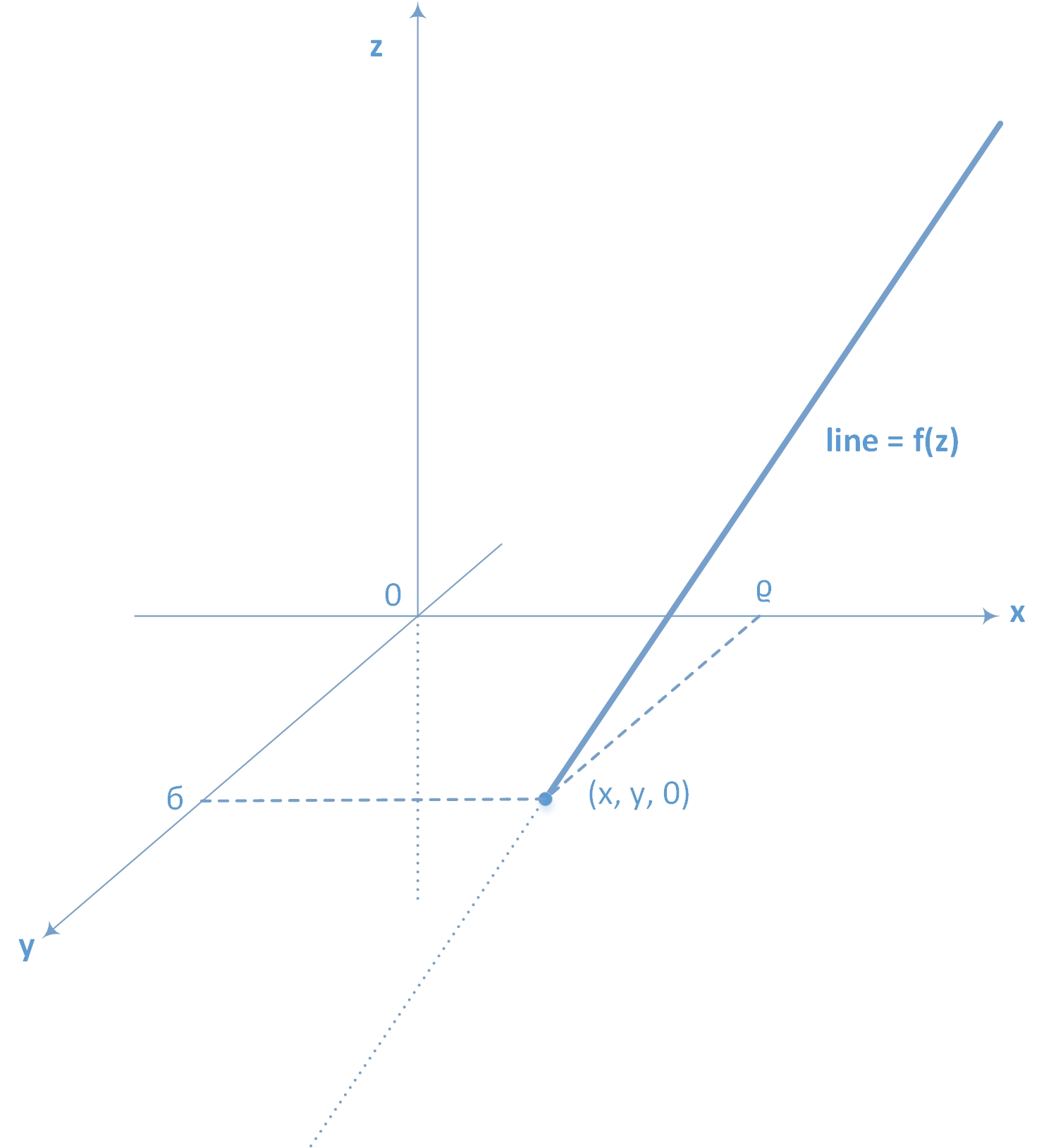
Figure 2: Notation used by Plücker, or Lie.

Of course, this is sufficient to describe the intersection point $\rho,\sigma$ at $z=0$, and due to the slopes $r$ and $s$ (i.e. the slopes of the planar projections of the line onto the respective coordinate planes) the line is determined throughout space and $\forall z$. One can also generalize this description versus analysis by setting $x=f_{1}(z)$ and $y=f_{2}(z)$ where $f_{1}(z)=rz+\rho$ and $f_{2}=sz+\sigma$ describe the simplest, linear case, and one can think about other functional dependencies $f_{i}(z)$, also about switching to $z\in\mathbbm{C}$ and performing analysis, relating geometrical pictures like the stereographic projection, etc. We have modified this approach using homogeneous coordinates to discuss spin and spinors, as well as aspects of special relativity with respect to the exceptional value $\eta=0$ (dahm:MRST7 and dahm:MRST8 , or sec. IV.1).

As we want to keep our focus on lines and different reps only, we do not follow these aspects. Here, it is more interesting with respect to relativity – which can be understood also to make claims on velocities with respect to our surrounding space-time – to introduce a point on the line and discuss linear motion. This can be seen from two sides:

• Given a point, acting with a force on the point will put the point into motion. Instead, we can assume also existing linear uniform motion and ask for the trajectory rep throughout time, which of course should yield a line rep in 3-space. So today, the usual rep in 3-space will consist of a 3-vector pointing from the coordinate origin to a point on the line, and a second 3-vector pointing in the direction of the force or the movement. In order to describe the point on the line, we thus have a 3-vector at ’time’ $t_{0}$ when we’ve ’started’ our process, and we can track the point using a parameter $t-t_{0}$, or $\Delta t$. So for all ’times’ $t\geq t_{0}$, we ’know’ the position of the point, however, we also know the integrated line as trajectory. So this picture ’lives’ from the fact that a line is a point set, and that we can tag the points on the line individually by an appropriate (linear) parametrization if in addition we accept ’velocities’ of the point on the line.

• An alternative geometrical view can be given by understanding a tagging of points on the line e.g. by its intersection with other known lines of a planar pencil, or even by known planes of a spatial pencil. So whereas on the one hand, we can construct lines as point sets (with at least two points), on the other hand the intersection of two lines, or a line by a plane, is by geometrical definition a point. In this picture, the movement of a point on a given line can be equally well parametrized by intersecting the line with a pencil of lines or planes, and individual points on the line are tagged by tagging the respective intersecting lines or planes, and by ordering the pencil elements appropriately. Instead of a ’coordinate system’ on the original line e.g. by a 3-vector and ’time’, we may use as well the coordinate system of the pencil and an additional rule (i.e. a mapping) related to the metric (if necessary). In the planar case, the line pencil (which we can e.g. take from a null system/Complex with the null point as center) and the original line should be coplanar, and the center of the pencil (in our example the null point) should not be incident with the original line (or analytically: $x_{i}l_{i}\neq 0$, where $x_{i}$ are ternary homogeneous point coordinates and $l_{i}$ are planar line coordinates). In other words, in this scenario the line $l$ shouldn’t be a null or Complex line. In case of the pencil of planes in 3-space, the axis of the pencil (i.e. the intersection of the planes) should be skew to the line of movement, so we can apply Congruences and null systems, too, or when introducing ’conjugation’, besides using null systems, we can introduce second order surfaces/quadrics, and apply polar theory and duality/reciprocity (i.e. symmetric matrix reps and ’anti-commutators’). Now, the points on the lines are annotated by an ’angle’ within the respective pencil related to fundamental rays or planes of the pencil, which we can describe by an anharmonic ratio (or better with von Staudt: as ’Wurf’). PG then yields several mechanisms to adopt this view to analytical and algebraical reps, typically by ’Würfe’ or anharmonic ratios, and by deriving metrical properties thereof, see e.g. Doehlemann doehlemann:1905 , III. Abschnitt.

Last not least, we may introduce and discuss ’velocities’ to denote the motion of the point on the line by different ’coordinate systems’, or simply by different reps. Whereas the original static picture $x=f_{1}(z)$ and $y=f_{2}(z)$ fails without further assumptions on a parameter dependence of $z$ and enhanced notation, we are used to think of a linearly moving point (i.e. a tagged point on a line!) in vector notation using point coordinates.

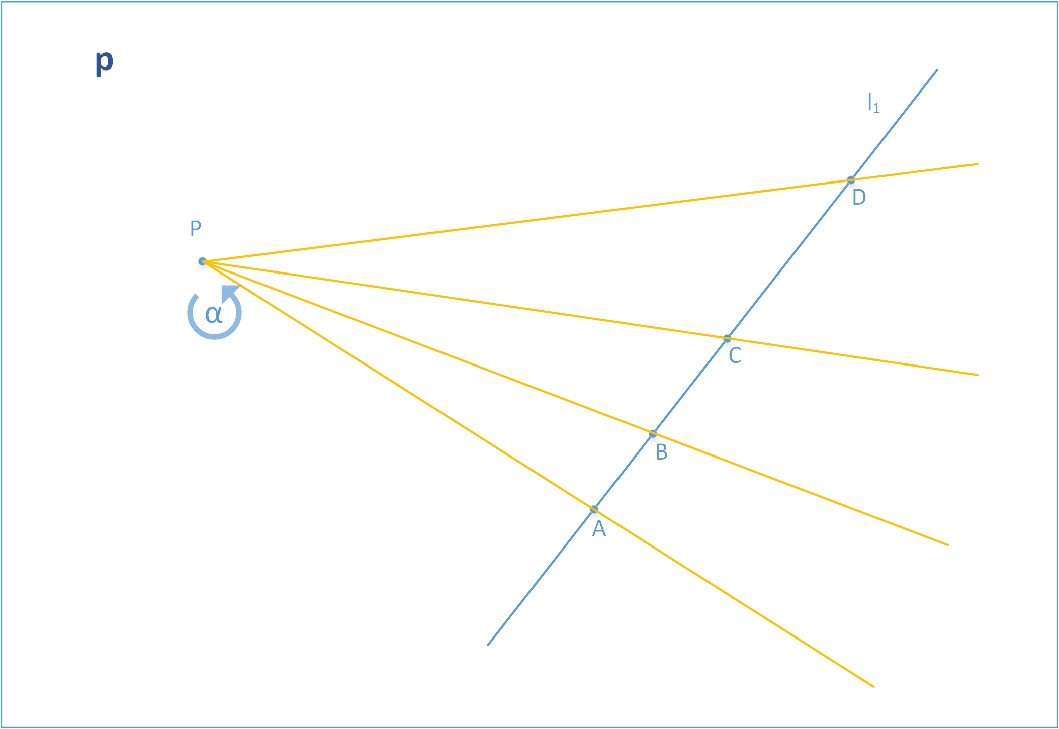
Figure 3: Points on a line $l_{1}$ versus a pencil coordinate $\alpha$.

So the adequate picture (see e.g. figure 3) – as soon as we interpret the direction of the line by associating it with a velocity vector. In terms of the line pencil, however, switching to the different parametrization, we have to interpret the coordinate of the planar line pencil as an angular velocity related to a rotation so that ’over time’ we measure different angles of $\alpha$. If we interpret the original motion as continuous, we have introduced, of course, once more a dependence of a ’time’ $t$, i.e. $\alpha(t)$. The same picture holds for null systems or Congruences if we use the angle between the planes.

Not that this switch is a problem, however, notation and the physical pictures change although they are, of course, related, and the relation between $\alpha$ and the position measured on the line – although nonlinear – can be given immediately because we know the respective functional dependencies from planar (or spatial) Euclidean geometry nowadays by heart, and we have even introduced names or naming of their groups like ’trigonometric functions’, ’hyperbolic functions’, ’HuppelDuppel’ functions or polynomials, etc.

Using this simple setup, we can already discuss various possibilities describing point velocities on the line $l_{1}$ versus pencil parameter $\alpha$:

• $\delta\alpha$ between pencil lines is constant per ’time’ interval, i.e. $\omega=\alpha t$. Switching to metric properties on $l$ and assuming common ’time’ $t$ for line and pencil yields that related distances on $l$ between intersections in the line metric are a priori NOT equal. If we introduce ’physics’ on the line (i.e. a velocity $v$ on the line $l$ with respect to the metric and synchronize clocks at the intersection points), we find an accelerated motion $\dot{v}\neq 0$.

• We can change the usual metric to a ’non-Euclidean metric’ on the line in that we require the distances between the intersection points on the line to be equidistant. Then in the linear picture, we can recover linear space and velocity, however, we have to pay the price with a strange (and for our common picture unusual) ’time definition’. Our understanding can be restored if we recall that a projective line can be understood as a special circle closing through ’infinity’ (i.e. by enhancing the Euclidean picture by an absolute element). Then, the line behaves as a circle around the center of the planar pencil. However, we have to switch to projective instead of Euclidean geometry only.

• As an alternative, we can absorb this ’strange’ behaviour by using different ’times’ on $l$ and on the rotating line of the pencil, so dependent on the metric on $l$ whether we require the distance or the velocity to be constant, this can be absorbed as well by different non-constant rotations, or even by non-linear ’times’.

So in general the notion of velocities is generated by identifying and tagging a special (sub-)element of a lower stage – the point on the line or the line or plane of the respective pencil – and recalling projective construction schemes. The ’velocity’ is introduced by the observation that the tagged elements evolve ’in time’ through the allowed (or a priori existent) positions of the superior element, i.e. the mapping itself can be understood to change ’in time’. In essence, we thus obtain different mappings between the line and the pencil by different identifications and transfer rules.

In order to gain some more insight into such constructions, we may assume a second line $l_{2}$, and if – by chance – it happens (see figure 4, or the discussions in dahm:MRST3 , dahm:MRST4 ) that the motion of a point on $l_{2}$ can be tagged in the same manner like the point motion on $l_{1}$, we can apply some fundamental theorems of planar projective geometry.

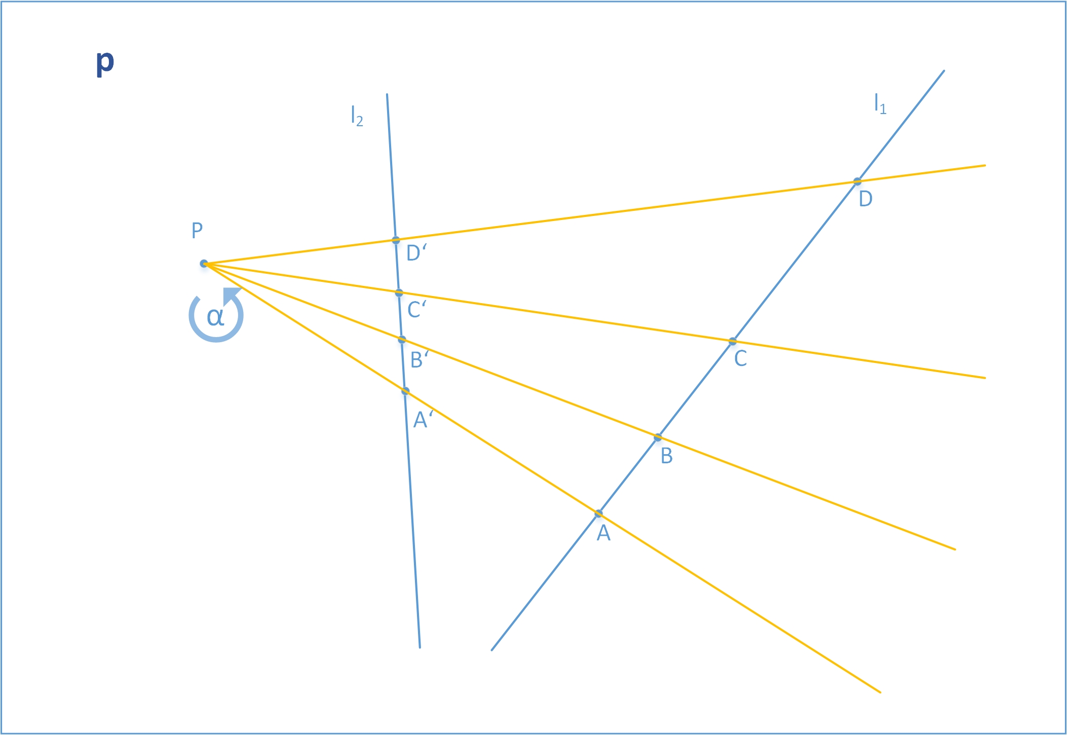
Figure 4: Points on two lines $l_{1}$ and $l_{2}$ with different velocities versus the same pencil coordinate $\alpha$.

The points are determined by linear sections of the same pencil which relates them, i.e. we can write a well-defined mapping down by means of the anharmonic ratios of point sets and lines although the individual ’velocitities’ on $l_{1}$ and $l_{2}$ are different. It is obvious, that this situation changes, if the points at the respective angles $\alpha_{i}$ do not coincide, or if – like in figure 5 –

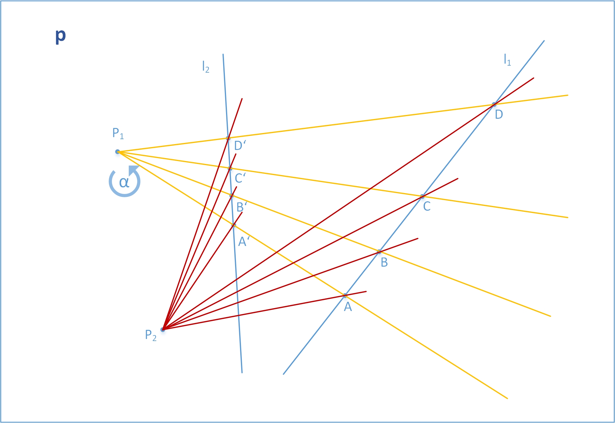
Figure 5: The same setup with two ’observers’.

there is a second ’observer’ at $P_{2}$. Nevertheless, we can discuss this planar setup by projective, or perspective mappings doehlemann:1905 , and use anharmonic ratios to describe and relate the setup parameters.

Last not least, leaving the planar setup and switching to lines in space, we have even two scenarios at hand:

The general setup we have discussed so far, are two skew lines where points are moving (see dahm:MRST3 , or dahm:MRST4 ). In this scenario, to connect (or relate) points, we cannot in general use only one planar pencil, but we have to discuss Congruences, or ’ray systems’, i.e. we need to consider at least two linear Complexe and their common lines. This illustrates why we can use the description of line geometry given above to treat Lorentz transformations and relativity.

The second (and related) scenario can be developed right from figure 5. With respect to ’the second observer’ at $P_{2}$, we may switch the lines $l_{1}$ and $l_{2}$ ’out of plane’ into different spatial positions. But now we can apply a construction scheme which Plücker has published pluecker:1847 as an alternative to Monge’s generation of a one-sheeted hyperboloid. Understanding $P_{2}$ as center/vertex of the original (planar) line pencil, the plane transforms into a one-sheeted hyperboloid while moving the lines out of the plane $p$. The two lines $l_{1}$ and $l_{2}$ (where their intersection points with the pencil remain fixed in the sense of a mechanical model/construction e.g. by filaments, or fibres), now positioned in space, belong to one of the family of generators whereas the intersecting lines belong to the second family. Plücker in pluecker:1847 discussed explicitly this filament/fibre model, and he categorizes his second class construction versus Monge’s construction as well as the rôle of duality. Especially with respect to cones, he emphasizes their singular/special character and comments on the relevance of duality.

As such, the notion of ’relativity’ in general can be associated to construction schemes in PG, and as such to the respective transfer principles. Moreover, it can be subsumed under Klein’s ’Erlanger Programm’. And it is obvious, that the parameter (or ’coordinate’) ’time’ has a different meaning by its tagging function than point reps in terms of pure spatial coordinates.

Appendix B Projective Generation and Fields

In addition, we want to recall a construction scheme of field reps in terms of circle pencils which is automatically introduced by the tetrahedral Complex and some transfer principles. We have mentioned above the relation of the tetrahedral Complex and the fundamental coordinate tetrahedron. It is also evident that lines in 3-space hit the planes of the coordinate tetrahedron in four points (the four planes opposite of the vertices of the tetrahedron, or within a self-polar fundamental coordinate tetrahedron the planes even dual to the vertices). Now by recalling that the tetrahedral Complex, a quadratic Complex, consists of all lines with the same anharmonic ratio $\kappa$ of the four intersection points with respect to the tetrahedron, we find an associated set of $\infty^{1}$ such ratios depending on different intersections of lines with the fundamental coordinate tetrahedron. In other words, given a fundamental tetrahedron of coordinates and an additional parameter, interpreted as the anharmonic ratio of the intersection points, one tetrahedral Complex is selected. Note that the anharmonic ratio is invariant under projective transformations of projection and intersection!

Now, if in the next step we take a line with its four intersection points, and if – in addition – we intersect the line with a plane, i.e. the line with its four points are all elements of the plane (i.e. incident with the plane), we can apply an interesting geometrical construction scheme doehlemann:1905 in order to attach pencils of circles and their orthogonal pencils. Because Doehlemann’s original purpose to investigate point involutions on the line by identifying the two carriers of the points is comprised, identifying point sets on the remaining common carrier, the line, yields an additional projective mapping, and a birational mapping of the individual ’parameters’ doehlemann:1905 §§17ff. Moreover, we thus can apply immediately the original framework of Hesse’s transfer principle to the point sets, use binary form reps and the associated differential equations clebsch:1872 which occur in various contexts in physics and especially ’quantum’ theories.

Here, we focus on the construction of circles and pencils of circles by using the line from the tetrahedral Complex with its four intersection points $A$, $B$, $A^{\prime}$, and $B^{\prime}$, with the fundamental tetrahedron. In addition, we associate a point $P$ off-line in the plane $p$ to avoid analytical problems with degeneracies for the moment (see figure 6). Physically, the point $P$ may be associated with a probe or an observer, and it is evident that with respect to the fundamental tetrahedron, we can either associate quaternary homogeneous space-coordinates of $P^{3}$, or switch to affine or Euclidean coordinates, i.e. we will find linear (or of order 1) reps of this point.

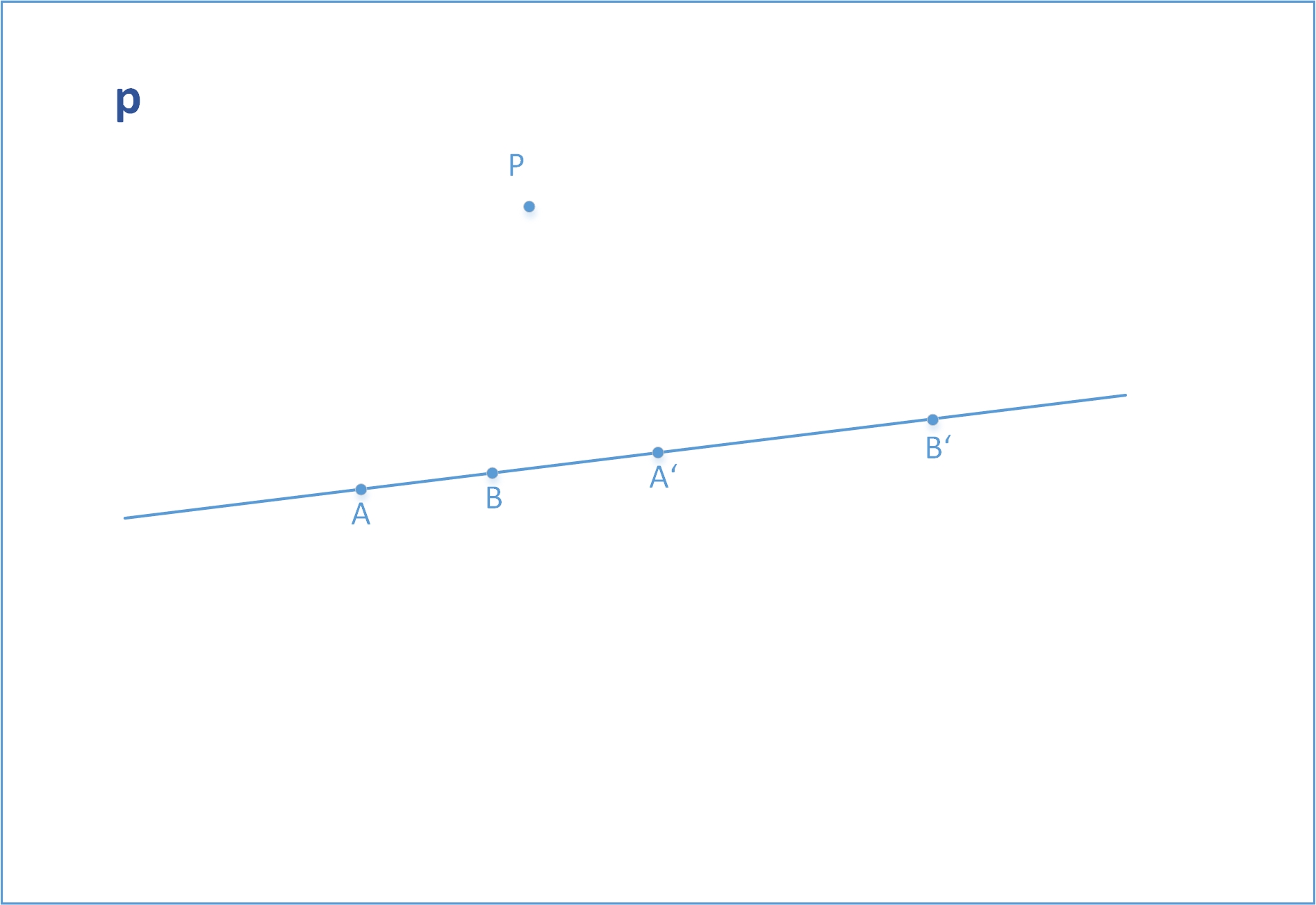
Figure 6: Step 1: Define point $P$ and plane $p$ with respect to the line, the four points $A$, $A^{\prime}$, $B$, $B^{\prime}$, and their anharmonic ratio $\kappa$.

However, if in the next step we intersect the point sets ($P$, $A$, $A^{\prime}$) and ($P$, $B$, $B^{\prime}$) by circles like in figure 7, we can denote the intersection point of the circles by $Q$ (see figure 8).

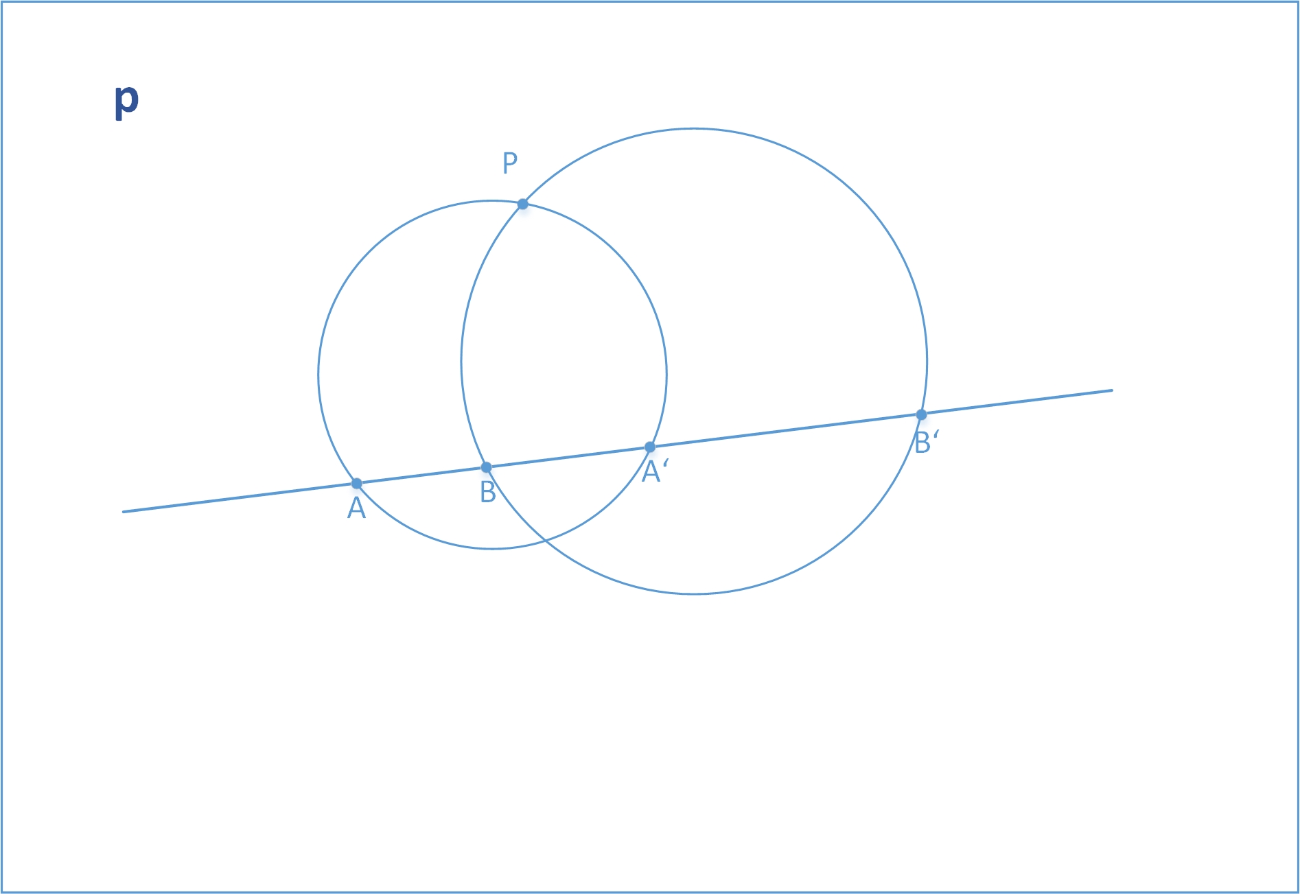
Figure 7: Step 2: Connect $P$ with the two point sets ($A$, $A^{\prime}$) and ($B$, $B^{\prime}$) by circles.

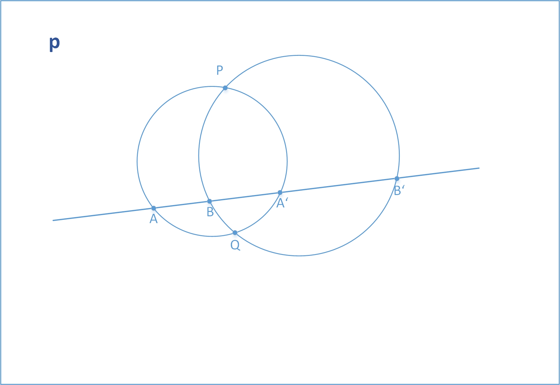
Figure 8: Step 3: Identify $Q$ as second intersection of the two circles.

For the upcoming steps, the line with the points $A$, $B$, $A^{\prime}$, and $B^{\prime}$ is no longer of direct use, but we draw all circles through the points $P$ and $Q$ like in figure 9.

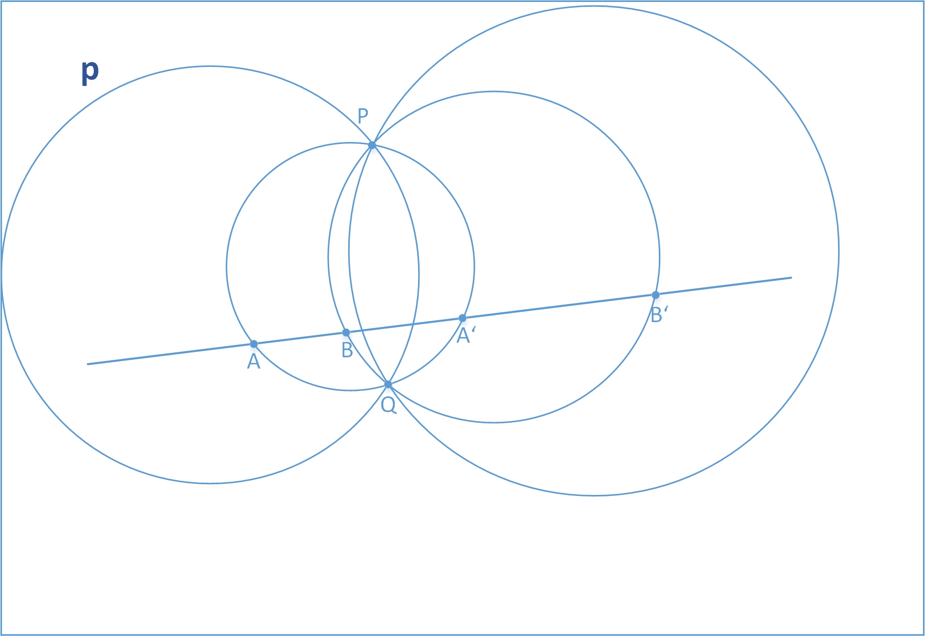
Figure 9: Step 4: Visualize the pencils of circles through $P$ and $Q$.

In this figure, we have drawn only few lines to recall the principle but it is evident that one can find planar circles connecting each planar point with $P$ and $Q$, i.e. we may attach (at least) one quadric rep to each planar point. So in Plücker’s sense, we may as well switch to a geometry using the circle as base element of this geometry.

In a last step to get closer to usual descriptions, it is helpful to change the planar coordinate system like in figure 10 where the first axis is a line incident with $P$ and $Q$, and we may choose the origin by an orthogonal axis half between $P$ and $Q$, i.e. in addition we can fix the orientation by the anharmonic ratio ($Q$,$0$,$P$,$\infty$)=-1.

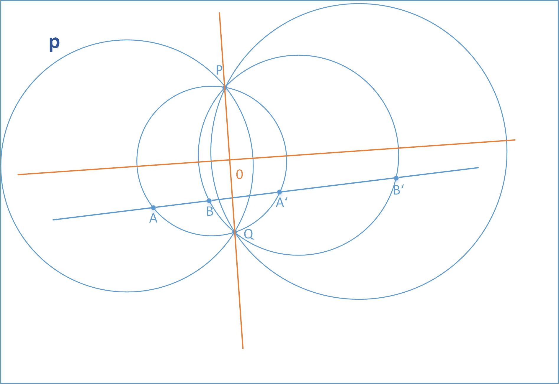
Figure 10: Step 5: Draw line through $P$ and $Q$, and an orthogonal line at $0$.

As a comparison, we want to refer to the picture in figure 11 as given in kleinHG:1926 when presenting pencils of circles and of orthogonal circles.

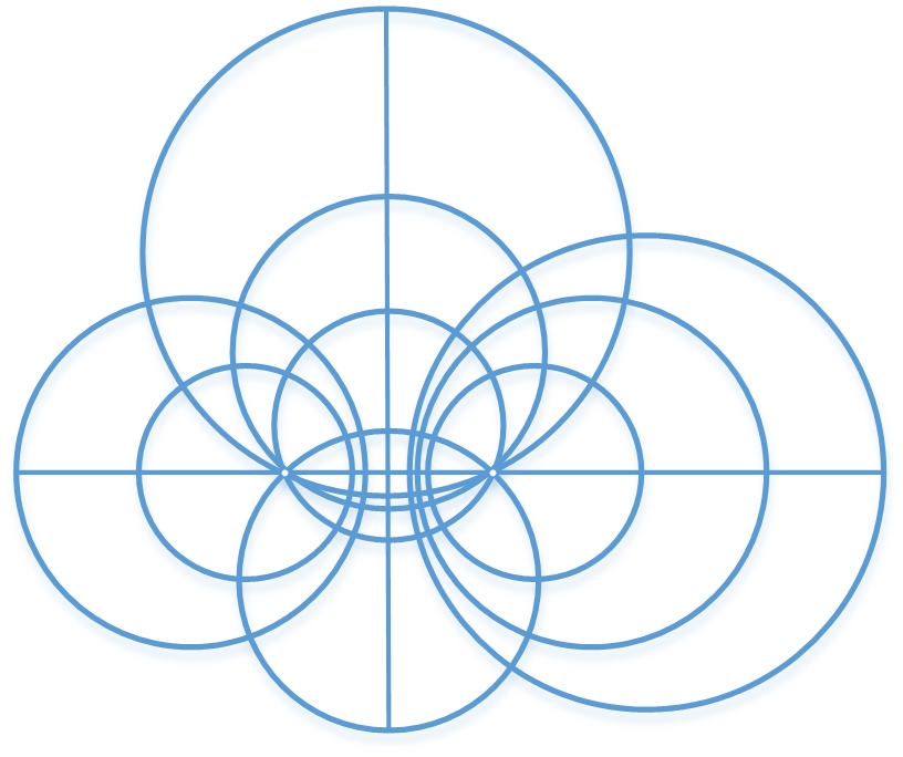
Figure 11: Comparison to FIG. 10: Pencils of original and orthogonal circles given by Klein kleinHG:1926 , p. 42.

Now if we recall $P$ representing originally a probe or an observer, we have introduced a description where the ’forces’ (or field line orientations’) point towards $Q$, but we can introduce in addition orthogonal sets of circles or conics to introduce the notion of ’potentials’. As most of this is classical analytical geometry, we leave it to the reader to play with conics and partial differential operators using incidence relations (due to tangential conditions) in the linear and the quadric case. Moreover, it is interesting to play with the ’two infinities’ of the rectangular axes and relate them to the scenario where the plane is the projection plane of a stereographic projection and both axes meet in a second point. Vice versa, one can think to replace $P$ and $Q$ by $\pm i$, and perform some algebra also with their anharmonic ratio versus $0$, and $\infty$.

Appendix C Complex Numbers and Geometry

Although it sounds silly to discuss nowadays complex numbers because everybody is used to work with them from scratch, it is worth to briefly recall their use by means of a simple geometrical example.

As example, one can write down the intersection of a circle and a line in planar coordinates where it doesn’t matter whether we use two Euclidean coordinates or three homogeneous planar coordinates. We obtain – of course – three cases to be distinguished:

1. the line hits the circle in two real points (’secant’),

2. the line is a tangent to the circle (one real double-point), or

3. the line misses the circle, i.e. there is no intersection in the Euclidean plane.

The analytic calculation to find the two intersection points by finding the two roots is well-known.

Now it is noteworthy, that exactly the physically not so interesting case where there is no intersection in the Euclidean plane requires to complex roots to treat the analytical rep in terms of coordinates. In other words, the complex numbers serve as an algebraic or analytic unification tool by introducing the symbol $i$ and appropriate rules to work with this symbol. In the planar case, this extension serves to treat two ’conjugate’ points on the absolute line, whereas in 3-space, we have to introduce additional symbols to treat a line or a plane vs. a second order surface. Based on Lie transfer and Study’s work in line geometry, we have discussed the construction of spinors in dahm:MRST7 by means of homogeneous coordinates while respecting the absolute elements and treating ’null’ elements. So it is justified to understand complex numbers (and quaternions, and in general hypercomplex numbers as well) as symbols to serve for algebraic/analytic completion when representing geometry and associating absolute elements in homogeneous coordinates to the respective geometries.

However, being physicist, when being asked to vote for the interesting case(s), I’d vote for a) and b) where the line meets the circle at least in one point and where the probability that ’something interesting happens’ seems to be much higher than in the non-intersecting case c). It seems justified to regard and understand the case c) as being necessary to complete the algebraic/analytic description formally, and to see whether the mathematical tool sets work appropriately or not – the more, as we can apply a lot of more unphysical ideas to this picture like shrinking the circle or even the line to a point, etc. which introduces ambiguities or even singularities.

Appendix D Einstein and ’Six-Vectors’

As brief and quick access to Einstein’s publications in order to guarantee a certain overview of the original concepts of special and general relativity, we’ve used publications of his talks in the transactions of the Prussian Academy of Science einstein:1914-32 during his time in Berlin as well as his publications in ’Annalen der Physik’ which we’ll discuss briefly with focus on the use of the ’six-vector’ in order to attach Complex geometry to special and general relativity as discussed nowadays by 4-vector calculus and differential geometry.

D.1 Prussian Academy of Science

Here, we’ve found three publications which we want to mention for later geometrical use.

In einstein:1914 Einstein mentions in a very small paragraph briefly ’six-vectors’ as an alternative notation in the context of $2^{nd}$-rank antisymmetric tensors (p. 1037/1038) without physical context. Only after having introduced the ’antisymmetric fundamental tensor of Ricci and Levi-Civita’ yielding

$$\begin{array}[]{lcl}G_{iklm}&=&\sqrt{g}\,\delta_{iklm},\\ G^{iklm}&=&\frac{1}{\sqrt{g}}\,\delta_{iklm},\quad\mathrm{and}\\ G^{lm}_{ik}&=&\sum_{\alpha\beta}\sqrt{g}\,\delta_{ik\alpha\beta}\,g^{\alpha l}g^{\beta m}\\ &=&\sum_{\alpha\beta}\frac{1}{\sqrt{g}}\,\delta_{lm\alpha\beta}\,g_{\alpha i}g_{\beta k}\end{array}$$ (59)

in eqns. (19), (21a), and (22), Einstein discusses the case of dual six-vectors in eq. (24),

$$(F^{\mu\nu})^{*}=\frac{1}{2}\sum_{\alpha\beta}G^{\mu\nu}_{\alpha\beta}F^{\alpha\beta}$$ (60)

with respect to the electromagnetic field rep. However, the whole discussion seems to focus mainly on tensor algebra. The major part of discussing $2^{nd}$-rank tensors throughout this contribution is related to symmetric tensors which yield 10 components and which in §9, p. 1055, is related as $T_{\sigma\nu}$ to the energy tensor. Because we do not want to discuss details here due to the focus on six-vectors (and Complexe or null systems), we just want to emphasize the connection of the symmetric part to polar systems and second order surfaces for later use.

In einstein:1916 , Einstein starts from Minkowski’s identification of the six electromagnetic field components as six-vector and discusses Maxwell’s equations. Einstein defines a ’new’ six-vector $\mathcal{F}^{\mu\nu}=\sqrt{-g}\sum_{\alpha\beta}g^{\mu\alpha}g^{\nu\beta}F_{\alpha\beta}$ which in case of special relativity reduces to the usual field components $\vec{h}$ and $-\vec{e}$ in order to incorporate electromagnetism into general relativity by means of the tensor $\mathcal{T}^{\nu}_{\sigma}$,

$$\mathcal{T}^{\nu}_{\sigma}=\sum_{\alpha\beta}\left(-\mathcal{F}^{\nu\alpha}F_{\sigma\alpha}+\frac{1}{4}\mathcal{F}^{\alpha\beta}F_{\alpha\beta}\delta^{\nu}_{\sigma}\,.\right)$$ (61)

From our point of view, it is important to note that throughout his calculations, he uses only the field tensor $F^{\alpha\beta}$, even in his generalized form $\mathcal{F}^{\alpha\beta}$ and in derived equations, i.e. one six-vector (or Complex).

In einstein:1932b , Einstein and Mayer decompose in §2 the antisymmetric $4\times 4$-tensor rep of $R^{4}$. By means of ’the totally antisymmetric tensor $\eta^{iklm}$’ they exercise an algebra which basically represents working with pairs of four-indices, and which in line geometry is related to switching ray versus axis coordinates. $\eta$ can be understood as a rep of the $4\times 4$-determinant when working with point or plane coordinates. As such, one obtains a rep of line coordinates and in consequence naturally Lorentz transformations (see the discussion above or dahm:MRST8 ).

D.2 Annalen der Physik

Within his publications throughout this journal, we’ve found only two places which seem to be related to Complexe, or to six-vectors. However, in both cases this seems to be a naming convention, and Einstein has made no real use of this geometry or related formalisms.

To be complete, we’ve found in his paper of 1905, titled ’Zur Elektrodynamik bewegter Körper’, §8, p. 913f, five times the expression ’Lichtkomplex’, i.e. a complex of light, however, without explanation or definition. So there is no evidence that Einstein referenced a line Complex, or whether he used some contemporary notion of describing light in a certain manner.

The other occurence, we’ve found in his paper on general relativity of 1916, titled ’Die Grundlagen der allgemeinen Relativitätstheorie’. There in §20, he discusses briefly the Maxwell equations of the electromagnetic field based on Minkowski’s rep theory, as he mentions.

Appendix E Remarks on Representation Theory and Lie Symmetries

E.1 Remarks

Throughout the text and the other appendices, we’ve switched ’on demand’ between classical and ’quantum’ reps of objects and operators. We have prepared in dahm:MRST6 a more detailed account, however, as we’ve used various aspects so far, we want to provide a brief overview(or summary) at least on the aspects in 3-space. From the viewpoint of classical geometry, the central aspects we’ve used are points, lines and planes, and we’ve discussed mappings where (besides a lot of other ’transfer principles’) duality is a central aspect. As such, within classical geometry of 3-space, we have to quaternary reps $x$ and $u$ with respect to points and planes, and besides mapping points to points, and planes to planes, we know correlations mapping points to planes, and vice versa. Lines map under duality to lines, we may use senary reps as above (or nowadays ’Grassmannians’ Gr(2,4)), so on the one hand, we have only a single line formalism, on the other hand, we automatically have to take care and work with quadratic forms a priori. As a sufficient framework, we can invoke classical projective and advanced geometry like discussed e.g. in kleinHG:1926 or literature cited there.

The classical approach, however, doesn’t provide a rep for what people started to discuss as ’quantum’ theories in terms of differential operators on Hilbert spaces, i.e. using function reps. First of all, we want to attach linear rep theory (or ’plane waves’), and in order to associate physical pictures, we need to find appropriate reps on function spaces, too. With respect to relativity, a suitable starting point in classical geometry of 3-space is the plane rep either in general form $Ax+By+Cz-D=0$ or in terms of Hesse’s implicit representation, i.e. if we define the plane as usual by all $\vec{x}$ which are normal to a given normal vector $\vec{n}$ in Euclidean 3-space, the plane $\textfrak{p}$ reads as $\textfrak{p}=\vec{n}\vec{x}-d$, where $d$ denotes an oriented distance of plane and origin. Now, in this picture we can replace the Euclidean coordinates, of course, by the known fractions of homogeneous coordinates above, so this plane can be rewritten either as $\textfrak{p}=Ax_{1}+Bx_{2}+Cx_{3}-Dx_{0}=0$ for the general form, or by $\textfrak{p}=n_{1}x_{1}+n_{2}x_{2}+n_{3}x_{3}-dx_{0}$ in Hesse form, which both formally resemble a ’Lorentz invariant’ product $\textfrak{p}=p_{\mu}x^{\mu}$. Now the ’4-momentum’ $p_{\mu}$ comprises the components $(p_{0}=d,n_{1},n_{2},n_{3})$, however, it is a quaternary plane rep which in classical geometry we can treat also as $u_{\alpha}$, and as such the $0$-component $p_{0}$ representing the oriented distance changes sign appropriately. As an example, in the case of a sphere with radius $r$, we have two parallel tangential planes at distance $\pm r$ at antipodal points of the sphere, and we have to take care only whether we discuss spherical or elliptical geometry, but we do not have to take care of ’anti-particles’ or ’time-reversal’. Note, however, that we have attached a special interpretation to the coordinates, and especially the $0$-coordinate denotes a metrical property. So the calculus itself has to be attached to normals and normal congruences which relates this rep theory on the one hand to Study’s summary paper study:1905 , on the other hand we are back again on the original ground of maps of normal Complexe (see lie:1896 and references therein).

If we specialize our coordinatization further with respect to a planar point in 3-space, in order to define the metric we have mentioned the usual procedure to use logarithms of anharmonic ratios of points. So using the above plane rep as argument of an exponential, and adding a phase $i$ to compensate the phase in the metric, yields reps according to $\exp\pm ip\cdot x$. As check, if we take the tangential point as origin, the vector $\vec{x}$ of planar points in 3-space is always perpendicular to the normal $\vec{p}$, so we the logarithm of the metric mapping yields the remaining $0$-component $p_{0}$ as metric distance. Acting with $\partial_{\alpha}$ on this rep yields $p_{\alpha}$, and we may use standards rules like known from QFT to multiply exponentials. As such, we can see $i\partial_{\alpha}$ as a phenomenological (however, restricted) replacement of quaternary plane reps on function spaces, especially since the plane exponential remains but produces a linear quaternary rep $i\partial_{\alpha}\exp(-ip\cdot x)\sim p_{\alpha}\exp(-ip\cdot x)$, and moreover, it yields according to its later processing e.g. in QFT the necessary information on ’momentum conservation’ within this rep. Formally, we can remember the geometrical relation of order and class, so we understand this ’plane wave’ rep as class view, however, one has to be careful with the physical interpretation of the components. So the axiomatic approach by first quantization can be understood as well by transferring classical geometry to function spaces, and integer numbers or multiples of $2\pi$ emerge automatically for certain geometric conditions of Complexe (or ’screws’) (see e.g. zindler1:1902 , ch. 1) or cones (second class surfaces), especially if the vertex is a point in the absolute plane, and we obtain a cylinder. The interpretation of ’currents’ or ’lines’ by means of such ’4-momenta’, however, is coincident with the senary line definition only if we respect Lie’s picture discussed in sec. IV.1, and visualized by figure 1, i.e. if we understand the normal as the direction of the senary line rep, or in terms of line elements to follow Lie’s presentation of differential geometry in 3-space.

Here, we’ve discussed this phenomenology with respect to identifications and linear reps used in various physical models and discussions. So far, we have reps for points and planes, however, with respect to Lie’s and Study’s refs cited above with respect to the normal systems of surfaces, we want to find also appropriate reps of lines and second order surfaces to gain control and to reproduce the construction schemes of projective geometry. So besides representing the line family sets of second order surfaces, it is interesting to have possibilities to investigate or even gain control on non-local behaviour. Wigner’s ’relativistic angular momentum operator $M_{\mu\nu}$’ in wigner:1962 shows dependence only with respect to one point coordinate rep, and Gilmore’s generator definitions (see e.g. gilmore:1974 , p. 450/451, eqns. (1.28s) or (1.28h)), given for the case SO($n$,1) according to $X_{ij}=x^{i}\partial_{j}-x^{j}\partial_{i}$, $X_{i,n+1}=x^{i}\partial_{n+1}+x^{n+1}\partial_{i}$, depend (like elsewhere when performing e.g. angular momentum algebra) only from one point rep $x$. However, right from the definitions above we see that the action of $\partial_{n+1}$ in this case produces an additional sign, and if we recall that we act on second order surfaces, we obviously perform the algebra of a special or even singular rep.

As such, we’ve defined for our use with respect to second order surfaces and (senary) line reps an a priori ’non-local’ operator

$$L_{\alpha\beta}=\frac{1}{2}\left(x_{\alpha}\frac{\partial}{{\partial y}_{\beta}}-x_{\beta}\frac{\partial}{{\partial y}_{\alpha}}\right)$$ (62)

which we can justify generally for two points $x$ and $y$ of a quadric $S(x)=a_{\alpha\beta}x_{\alpha}x_{\beta}$ because acting with this operator (on a canonical/’diagonal’ form of S) yields $L_{\alpha\beta}S=x_{\alpha}y_{\beta}-x_{\beta}y_{\alpha}$ which can be identified as $p_{\alpha\beta}$. So we have gained operator reps which by acting on second order surfaces behave as line coordinate reps $p_{\alpha\beta}$.

The typical differential discussion of taking two ’close’ points $x$ and $y$ on the quadric $S$ has to be modified due to the quaternary homogeneous coordinates used above, however, we can write at least symbolically $M_{\alpha\beta}=\lim\limits_{y\longrightarrow x}L_{\alpha\beta}$ and relate to Wigner’s ’relativistic angular momentum’ and to usual angular momentum algebra. As such, we discuss details in dahm:MRST6 but right now, one can try to understand Schrödinger equations or Klein-Gordon equations by the class view and planar reps in 3-space.

If – as an example – we calculate the commutator $[L_{\alpha\beta},L_{\gamma\delta}]$ of the ’line operators’, we obtain

$$\begin{array}[]{ll}4\left[L_{\alpha\beta},L_{\gamma\delta}\right]\,=&\hphantom{+}\delta_{\beta\delta}\left(x_{\gamma}\frac{\partial}{{\partial x}_{\alpha}}-x_{\alpha}\frac{\partial}{{\partial x}_{\gamma}}\right)\\ &+\delta_{\alpha\gamma}\left(y_{\delta}\frac{\partial}{{\partial y}_{\beta}}-y_{\beta}\frac{\partial}{{\partial y}_{\delta}}\right)\,.\end{array}$$ (63)

For $y\longrightarrow x$, this yields

$$\begin{array}[]{rl}4\left[L_{\alpha\beta},L_{\gamma\delta}\right]\,=&\left(\delta_{\beta\delta}\,\delta_{\gamma\rho}\delta_{\alpha\sigma}+\delta_{\alpha\gamma}\,\delta_{\delta\rho}\delta_{\beta\sigma}\right)\cdot\\ &\cdot\left(x_{\rho}\frac{\partial}{{\partial x}_{\sigma}}-x_{\sigma}\frac{\partial}{{\partial x}_{\rho}}\right)\\ \,=&2\left(\delta_{\beta\delta}\,\delta_{\gamma\rho}\delta_{\alpha\sigma}+\delta_{\alpha\gamma}\,\delta_{\delta\rho}\delta_{\beta\sigma}\right)L_{\rho\sigma}\,,\end{array}$$ (64)

and finally

$$\left[L_{\alpha\beta},L_{\gamma\delta}\right]\,=\,\frac{1}{2}\left(\delta_{\beta\delta}\,\delta_{\gamma\rho}\delta_{\alpha\sigma}+\delta_{\alpha\gamma}\,\delta_{\delta\rho}\delta_{\beta\sigma}\right)L_{\rho\sigma}\,.$$ (65)

The remaining operators on the rhs show the form of standard Lie generators of compact groups (see also Gilmore’s operator definitions cited above), and due to the quaternary indices, we are concerned with so(4). However, the intricate factor in front of the operators depends on Kronecker symbols of indices and restricts the algebra, and we have to resolve the result and its background by line geometry. This, however, is ongoing, and so far we do not have appropriate results from ’classical’ line geometry to compare to.

References

References

- (1) De Alfaro V, Fubini S, Furlan G, and Rossetti C 1973 Currents in Hadron Physics. (Amsterdam, London: North Holland Publishing Company)
- (2) Ball R S 1876. The Theory of Screws: A Study in the Dynamics of a Rigid Body. (Dublin: Hodges, Foster, and Co., Grafton-Street)
- (3) Biedenharn L C, Louck J D 1981. Angular Momentum in Quantum Physics. Theory and Application. (Encyclopedia of Mathematics and Its Applications) ed. Gian-Carlo Rota. (vol. 8, Reading: Addison-Wesley Publishing Company) (1981)
- (4) Biedenharn L C, Louck J D 1981. The Racah-Wigner Algebra in Quantum Theory. (Encyclopedia of Mathematics and Its Applications) ed. Gian-Carlo Rota. (vol. 9, Reading: Addison-Wesley Publishing Company) (1981)
- (5) Catto S 2019. Closing plenary talk at ISQS 26, Prague, July 2019, and private communication.
- (6) Clebsch A 1870. Ueber die Plückerschen Complexe. Math. Ann. 2 1
- (7) Clebsch A 1872. Theorie der binären algebraischen Formen. (Leipzig: B. G. Teubner)
- (8) Dahm R, Kirchbach M, Riska D O 1992. SU(4) Supermultiplet Description of the -System at Low Energies and Particle Interpretation in Effective Lagrangeans. Proceedings, Dubna, 1993
- (9) Dahm R, Kirchbach M, Riska D O 1993. Wigner Supermultiplets in –Photoproduction at Threshold. Invited Talk at the International Workshop on ’Symmetry Methods in Physics’, in memory of Professor Ya. A. Smorodinsky, Dubna, Russia, July 6 – 10, 1993. Proceedings, Dubna, 1994
- (10) Dahm R, Kirchbach M 1994. Linear Wave Equations and Effective Lagrangeans for Wigner Supermultiplets. Int. J. Mod. Phys. A10, 4225
- (11) Dahm R, Kirchbach M 1995. The Large -Limit of QCD and Effective Lagrangeans for Spin-Flavour Supermultiplets. ed. M. Kh. Khankhasayev, Zh. B. Kurmanov (Singapore: World Scientific) (1995)
- (12) Dahm R 1996. Spin-Flavour-Symmetrien und das N-System (Aachen: Shaker Verlag) ISBN 3-8265-1782-2
- (13) Dahm R 1995 Relativistic SU(4) and Quaternions Advances in Applied Clifford Algebra 7(S) 337
- (14) Dahm R 2010. A Symmetry Reduction Scheme of the Dirac Algebra without Dimensional Defects. Yad. Fis. 73 297; Phys. Atom. Nuclei 73 276
- (15) Dahm R 2012. On A Microscopic Representation of Space-Time. Yad. Fis. 75 1244; Phys. Atom. Nuclei 75 1173
- (16) Dahm R 2018 On A Microscopic Representation of Space-Time III. Adv. Appl. Clifford Algebras 29 20; https://doi.org/10.1007/s00006-018-0936-x; see also http://arxiv.org/abs/1508.06872
- (17) Dahm R 2015. On A Microscopic Representation of Space-Time IV. Phys. Atom. Nuclei 80, 512 (2017) QTS 9, Yerevan, http://arxiv.org/abs/1512.07119
- (18) Dahm R 2016. On A Microscopic Representation of Space-Time V. ISQS, Prague, Journal of Physics : Conference Series 804 012013 (2017)
- (19) Dahm R 2016. On A Microscopic Representation of Space-Time VI – A Stopover. to be published (2020)
- (20) Dahm R 2018. On A Microscopic Representation of Space-Time VII – On Spin. J. Phys.: Conf. Ser. 965 012012
- (21) Dahm R 2018 On A Microscopic Representation of Space-Time VIII – On Relativity. Phys. Atom. Nuclei 81 819
- (22) Dahm R 2019 On A Microscopic Representation of Space-Time IX – On Spin II. J. Phys.: Conf. Ser. 1194 012023
- (23) Dahm R 2019. Talk at ISQS 26. Prague, July 2019
- (24) Doehlemann K 1905. Projektive Geometrie in synthetischer Behandlung. (Sammlung Göschen) (3rd edition, Leipzig: G. J. Göschen’sche Verlagshandlung) (1898)
- (25) Dirac P A M 1935. The Electron Wave Equation in De-Sitter Space. Annals of Mathematics 36 657
- (26) Dirac P A M 1936. Wave Equations in Conformal Space. Annals of Mathematics 37 429
- (27) Dvoeglazov V V 1993. Lagrangean Formulation of the Joos-Weinberg’s 2(2S+1)-Theory and Its Connections with the Skew-Symmetric Tensor Description. Preprint:IFUNAM FT93-016, May 1993
- (28) Dvoeglazov V V 1993. The 2(2S+1)-Formalism and Its Connection with Other Descriptions. arXiv:hep-th/9305141v2, 1993/2016
- (29) Dvoeglazov V V 1993. Electrodynamics with Weinberg’s Photons. arXiv:hep-th/9306108v1, 1993
- (30) Dvoeglazov V V 1994. 2(2S+1)-Component Model and Its Connection with Other Field Theories. arXiv:hep-th/9401043v3; Preprint:IFUNAM FT-94-36, January 1994
- (31) Dvoeglazov V V 2018. Methods for Derivation of Generalized Equations in the Representations of the Lorentz Group. arXiv:1810.0458v1, 2018
- (32) Ehlers J, Pirani F and Schild A 1972. The Geometry of Free Fall and Light Propagation. In: Studies in Relativity. ed L O’Raifeartaigh (Oxford: Clarendon Press) pp 63–84
- (33) Einstein A 1914/1932. Albert Einstein: Akademie-Vorträge. ed D Simon (Weinheim: WILEY-VCH Verlag GmbH & Co. KGaA)
- (34) Einstein A 1914. Die formale Grundlage der allgemeinen Relativitätstheorie. Sitzungsberichte der königlich Preussischen Akademie der Wissenschaften, Berlin, SB II, XLI, 1030
- (35) Einstein A 1916. Eine neue formale Deutung der Maxwellschen Feldgleichungen der Elektrodynamik. Sitzungsberichte der königlich Preussischen Akademie der Wissenschaften, Berlin, SB I, VII, 184
- (36) Einstein A, Mayer W 1932. Semi-Vektoren und Spinoren. Sonderausgabe aus den Sitzungsberichten der Preussischen Akademie der Wissenschaften, Physikalisch-Mathematische Klasse, Berlin, SB I, XXXII, 522
- (37) Gilmore R 1974. Lie Groups, Lie Algebras and Some of Their Applications (New York: John Wiley & Sons)
- (38) Helgason S 1978 Differential Geometry, Lie Groups, and Symmetric Spaces (San Diego: Academic Press)
- (39) Helgason S 1984 Groups and Geometric Analysis. (San Diego: Academic Press)
- (40) Hesse O 1866. Ein Uebertragungsprincip. Journal für die reine und angewandte Mathematik 66, 15
- (41) Hilbert D 1909. Ueber die Gestalt einer Fläche 4ter Ordnung. Göttinger Nachrichten 1909 308
- (42) Hilbert D 1915. Die Grundlagen der Physik. (Erste Mitteilung.) Göttinger Nachrichten 1915 395
- (43) Hilbert D 1916. Die Grundlagen der Physik. (Zweite Mitteilung.) Göttinger Nachrichten 1916 53
- (44) Hilbert D 1924. Die Grundlagen der Physik. Math. Ann. 92 1
- (45) Hudson R W H T 1905. Kummer’s Quartic Surface. (Cambridge Mathematical Library) (Cambridge: Cambridge University Press, 1990)
- (46) Joos H 1962. Zur Darstellungstheorie der inhomogenen Lorentzgruppe als Grundlage quantenmechanischer Kinematik. Fortschr. Phys. 10, 65
- (47) Klein F 1871. Notiz betreffend den Zusammenhang der Linien-Geometrie mit der Mechanik starrer Körper. Math. Ann. 4 403
- (48) Klein F 1872. Ueber Liniengeometrie und metrische Geometrie. Math. Ann. 5, 257
- (49) Klein F, Sommerfeld A 1897. Über die Theorie des Kreisels. Heft I (Leipzig: B. G. Teubner)
- (50) Klein F, Sommerfeld A 1898. Über die Theorie des Kreisels. Heft II (Leipzig: B. G. Teubner)
- (51) Klein F 1906. Zur Schraubentheorie von Sir Robert Ball. Math. Ann. 62, 419
- (52) Klein F 1910. Über die geometrischen Grundlagen der Lorentzgruppe. Jahresberichte Deutsche Math. Vereinigung 19 281
- (53) Klein F 1917. Zu Hilberts erster Note über die Grundlagen der Physik. Göttinger Nachrichten 1917 469
- (54) Klein F 1926. Vorlesungen über höhere Geometrie. (Die Grundlehren der mathematischen Wissenschaft XXII) (Berlin: Springer)
- (55) Kummer E E 1866. Über die algebraischen Strahlensysteme, in’s Besondere über die der ersten und zweiten Ordnung. Abh. Akad. Wiss. Berlin, Math. Abhandlungen, 1
- (56) Lie S 1872. Ueber Complexe, insbesondere Linien- und Kugel-Complexe, mit Anwendung auf die Theorie partieller Differential-Gleichungen. Math. Ann. 5 145; Ueber einige partielle Differential-Gleichungen zweiter Ordnung. Math. Ann. 5 209
- (57) Lie S 1896. Geometrie der Berührungstransformationen. (Leipzig: Teubner)
- (58) Lüroth O 1867. Zur Theorie der windschiefen Flächen. Journal für die reine und angewandte Mathematik 67, 130 (1867)
- (59) Minkowski H 1910. Die Grundgleichungen für die elektromagnetischen Vorgänge in bewegten Körpern. Math. Ann. 68, 472
- (60) Pauli W 1933 Über die Formulierung der Naturgesetze mit fünf homogenen Koordinaten. Teil I: Klassische Theorie. Annalen der Physik 18 305
- (61) Pauli W 1933 Über die Formulierung der Naturgesetze mit fünf homogenen Koordinaten. Teil II: Die Diracschen Gleichungen für die Materiewellen. Annalen der Physik 18 337
- (62) Plücker J 1838 Discussion de la forme générale des ondes lumineuses. Journal für die reine und angewandte Mathematik 19 1; ibd. 19 91
- (63) Plücker J 1847 Über eine neue mechanische Erzeugung der Flächen zweiter Ordnung und Classe. Journal für die reine und angewandte Mathematik 34 357
- (64) Plücker J 1865. On a new Geometry of Space. Phil. Trans. R. Soc. London 155 725
- (65) Plücker J 1866. Fundamental Views regarding Mechanics. Phil. Trans. R. Soc. London 156 361
- (66) Plücker J 1868/1869. Neue Geometrie des Raumes. ed A Clebsch and F Klein (Leipzig: B. G. Teubner)
- (67) Poincaré H. http://henripoincarepapers.univ-lorraine.fr/, as of 31.7.2019
- (68) Schmeikal B 2018. Private discussions
- (69) Sexl R U, Urbantke H K 1992. Relativität, Gruppen, Teilchen. (3rd edition, Wien New York: Springer)
- (70) Smorodinskij Ya A 1965. Kinematik und Lobatschewski–Geometrie. Fortschr. Phys. 13, 157 [Atomnaja Energija 14, 110 (1963)]
- (71) Staude O 1894. Ueber permanente Rotationsaxen bei der Bewegung eines schweren Körpers um einen festen Punkt. Journal für die reine und angewandte Mathematik 113, 318
- (72) Staude O 1905. Analytische Geometrie des Punktes, der geraden Linie und der Ebene. (B. G. Teubner’s Lehrbücher der Mathematischen Wissenschaften XVI) (Leipzig: B. G. Teubner, 1905)
- (73) Study E 1903. Geometrie der Dynamen. (Leipzig: Teubner)
- (74) Study E 1905. Über Hamiltons geometrische Optik und deren Beziehung zur Theorie der Berührungstransformationen. Jahresberichte Deutsche Math. Vereinigung 14 424
- (75) Tiwari S C 2012. On local duality invariance in electromagnetism. arXiv:1110.5511v2 physics.gen-ph, 2011
- (76) Trehub A. https://people.umass.edu/trehub/, as of 31.7.2019
- (77) Veblen O, Hoffmann B 1930. Projective Relativity. Phys. Rev. 36 810
- (78) Veblen O 1933. Projektive Relativitätstheorie. (Ergebnisse der Mathematik und ihrer Grenzgebiete) (Berlin: Springer)
- (79) Veblen O 1933. Spinors in Projective Relativity. Proc. Nat. Acad. Sciences 19 979
- (80) von Laue M 1950. Zur Minkowskischen Elektrodynamik der bewegten Körper. Z. Physik 128, 387 (1950), doi:10.1007/BF01339439
- (81) Weinberg St 1964. Feynman Rules for Any Spin. Phys. Rev. 133, B1318 (1964)
- (82) Weinberg St 1964. Feynman Rules for Any Spin. II. Massless particles. Phys. Rev. 134, B882 (1964)
- (83) Weinberg St 1965. Photons and Gravitons in Perturbation Theory: Derivation of Maxwell’s and Einstein’s Equation. Phys. Rev. 138, B988 (1965)
- (84) Weyl H 1918. Raum-Zeit-Materie. (6th ed. Berlin Heidelberg New York: Springer, 1970 (1918))
- (85) Wigner E P 1962. Invariant Quantum Mechanical Equations of Motion. In: Theoretical Physics, Lectures presented at the Seminar on Theoretical Physics, Trieste (Vienna, International Atomic Energy Agency 1963)
- (86) Zindler K 1902. Liniengeometrie mit Anwendungen. (Sammlung Schubert XXXIV) (Leipzig: G. J. Göschensche Verlagshandlung)
- (87) Zindler K 1906. Liniengeometrie mit Anwendungen. (Sammlung Schubert LI) (Leipzig: G. J. Göschensche Verlagshandlung)