Justifying Kubo’s formula for gapped systems at zero temperature: a brief review and some new results

Abstract

We first review the problem of a rigorous justification of Kubo’s formula for transport coefficients in gapped extended Hamiltonian quantum systems at zero temperature. In particular, the theoretical understanding of the quantum Hall effect rests on the validity of Kubo’s formula for such systems, a connection that we review briefly as well. We then highlight an approach to linear response theory based on non-equilibrium almost-stationary states (NEASS) and on a corresponding adiabatic theorem for such systems that was recently proposed and worked out by one of us in [51] for interacting fermionic systems on finite lattices. In the second part of our paper we show how to lift the results of [51] to infinite systems by taking a thermodynamic limit.

Keywords. Linear response theory, Kubo formula, adiabatic theorem, non-equilibrium stationary state.

AMS Mathematics Subject Classification (2010). 81Q15; 81Q20; 81V70.

1 Introduction

In this article we discuss the problem of “proving Kubo’s formula” for gapped extended quantum systems at zero temperature, with transport theory in (topological) insulators as the main application in mind. Note that in this context various expressions are referred to as “Kubo’s formula”, namely the general Kubo formula (KF) for the response coefficients of arbitrary observables on the one hand, and the double commutator formula (DCF) for the current response on the other. Thus also different mathematical problems have been subsumed under the label “proving Kubo’s formula”. As to be detailed below, much attention has been given to the problems of showing that KF implies DCF for the conductance or conductivity and to showing that DCF implies (fractional) quantisation of Hall conductance resp. conductivity (see e.g. the recent review [4] and references therein). Less work has been directed towards a rigorous justification of KF for such systems starting from first principles. As the present work will be mainly concerned with this second problem, let us briefly recall the main challenges such a justification faces.

In the context of Hamiltonian quantum systems, the linear response formalism for static perturbations answers the following question: How does a system described by a Hamiltonian $H_{0}$ that is initially in an equilibrium state $\rho_{0}$ respond to a small static perturbation $\varepsilon V$? Or somewhat more precisely: What is the change

$${\mathrm{tr}}(\rho_{\varepsilon}A)-{\mathrm{tr}}(\rho_{0}A)=\varepsilon\,\sigma_{A}+o(\varepsilon)$$

of the expectation value of an observable $A$ caused by the perturbation $\varepsilon V$ at leading order in its strength $|\varepsilon|\ll 1$? Here $\rho_{\varepsilon}$ denotes the state of the system after the perturbation has been turned on adiabatically and $\sigma_{A}$ is called the linear response coefficient for $A$. The answer clearly hinges on the problem of determining $\rho_{\varepsilon}$. While in some situations one expects that $\rho_{\varepsilon}$ remains an equilibrium state also for the perturbed Hamiltonian $H_{\varepsilon}=H_{0}+\varepsilon V$, Kubo [33] developed linear response theory for situations, where the system is driven into a non-equilibrium state $\rho_{\varepsilon}$. As emphasized by Simon in “Fifteen problems in mathematical physics” [49], the latter situation typically occurs in applications to transport theory and this deviation from equilibrium makes the justification of Kubo’s formula a difficult mathematical problem that is still not solved in satisfactory generality. Also in this work we will not even discuss the general problem but instead focus on the rather special situation of particle transport in gapped Hamiltonian systems (i.e. insulators) at zero temperature. In this case all currents are dissipation-less (direct currents vanish, while Hall currents are geometric and thus dissipation-less) and, as we will argue, a rigorous justification of Kubo’s formula purely on the level of Hamiltonian dynamics without involving any form of dissipation is possible.

The linear response formalism (which we briefly review in Section 2) rests on the assumption that a small perturbation ($|\varepsilon|\ll 1$) that is adiabatically switched on alters the initial equilibrium state of a system only a little ($\rho_{\varepsilon}\approx\rho_{0}$). In a nutshell, the problem of proving Kubo’s formula will thus be to prove that a system initially in an equilibrium state $\rho_{0}$ is adiabatically driven by a small perturbation into a non-equilibrium state $\rho_{\varepsilon}$ close to $\rho_{0}$. This problem goes beyond standard perturbation theory, since the small perturbation acts over a very long (macroscopic) time, and thus this assumed small change of the state is not a trivial consequence of the smallness of the perturbation; instead, proving this assumption requires an adiabatic type theorem. However, even if we work at zero temperature and assume that $\rho_{0}$ is the gapped ground state of $H_{0}$, the problem goes also beyond standard adiabatic theory. Indeed, the standard adiabatic theorem is only of rather limited use here for three reasons. First, it is only applicable as long as the perturbation does not close the spectral gap; then it asserts that $\rho_{\varepsilon}$ equals the gapped ground state of $H_{\varepsilon}=H_{0}+\varepsilon V$ and thus remains an equilibrium state. But, as emphasized before, in transport theory this assumption is often not satisfied and $\rho_{\varepsilon}$ is expected to be a non-equilibrium state; for example, the band gap in a typical insulator is of order 10eV, while a macroscopic sample of such a material stays insulating for applied voltages that are larger by many orders of magnitude. Secondly, even if one assumes that the spectral gap above the ground state remains open, the usual adiabatic theorem is not directly applicable for two reasons: its standard version estimates the difference between $\rho_{\varepsilon}$ and the ground state of $H_{\varepsilon}$ in the operator norm; in order to obtain the required estimates with respect to local trace norms, additional and potentially non-trivial propagation estimates need to be established. Finally, for extended interacting systems the approximation error in the adiabatic theorem deteriorates when the system size grows and it can not be applied for macroscopic systems. As a consequence, proving Kubo’s formula even in the simple case of gapped Hamiltonian systems at zero temperature has been an open problem of mathematical physics for quite some time.

Recently Bachmann et al. [8] proved an adiabatic theorem for extended interacting lattice systems with error estimates for local traces that are uniform in the system size, thereby solving the second and third problem. In [51] one of us solved also the first problem by proving a version of the adiabatic theorem that remains valid even when the perturbation closes the spectral gap. In a nutshell, the idea in [51] is that perturbations by slowly varying but not small potentials (modelling small fields acting on large regions of space) close the spectral gap, but leave intact a local gap structure, thereby driving the system into a non-equilibrium almost-stationary state (NEASS). The adiabatic theorem in [51] states that if such a perturbation is switched on adiabatically, then the state of the system evolves into a uniquely determined NEASS associated with the perturbed Hamiltonian that has an explicit asymptotic expansion in powers of $\varepsilon$; [51] also applies to interacting extended lattice systems and provides error estimates that are uniform in the system size. This NEASS approach was motivated by and is based on ideas which we called space-adiabatic perturbation theory almost 20 years ago, see for example [45, 46, 52], and allows not only to prove validity of Kubo’s formula, but also to evaluate it in a straightforward way. The latter point is illustrated in [37], where we compute the spin-Hall conductivity in topological insulators.

The rest of this note is structured as follows. Section 2 first recalls the formal derivation of Kubo’s formula in the context of Hamiltonian quantum systems and highlights the different mathematical problems arising from it. In particular, we try to clarify the different meanings that the phrase “proving Kubo’s formula” acquired in the past. We then try to provide a concise and structured overview of the mathematical literature in this area.

In Section 3, we discuss the extension of the results in [51] to infinite systems. We show that NEASSs exist as states on the quasi-local algebra of the infinite systems and are automorphically equivalent to the ground state of the unperturbed Hamiltonian, then state a version of a corresponding adiabatic theorem, and finally obtain from there a rigorous justification of an infinite volume version of Kubo’s formula. Proofs and generalizations of the results presented in Section 3 will be given elsewhere [29].

Acknowledgements: I (S.T.) would like to thank Yosi Avron, Sven Bachmann, Horia Cornean, Giuseppe De Nittis, Wojciech De Roeck, Alexander Elgart, Martin Fraas, Jürg Fröhlich, Vojkan Jaksic, Max Lein, Giovanna Marcelli, Domenico Monaco, Gianluca Panati, Marcello Porta, and Marcel Schaub for sharing their insights and ideas about this complex topic with me and/or for critically commenting on some of my own ideas.

2 Linear response: heuristics, problems, and results

In this section we first recall the standard derivation of the general Kubo formula for Hamiltonian quantum systems and static perturbations. We then highlight the steps in the derivation that require a more careful justification. In Subsections 2.1–2.3 we discuss some existing (mostly) mathematical literature addressing the different aspects of the problem.

Consider a quantum system described by the self-adjoint Hamiltonian $H_{0}$ on some Hilbert space $\mathcal{H}$ that is bounded from below and subject to a perturbation $\varepsilon V$ with $|\varepsilon|\ll 1$ such that also $H_{\varepsilon}=H_{0}+\varepsilon V$ is self-adjoint. The simplest example to keep in mind would be a single atom perturbed by a small external field, while relevant to transport theory are for example Hamiltonians describing fermions on a lattice with short range interactions subject to a perturbation by a small external field. Assume that initially, i.e. before the perturbation is applied, the system is in an equilibrium state $\rho_{0}$, i.e. $\rho_{0}\sim{\mathrm{e}}^{-\beta H_{0}}$ if the temperature $T=(k_{\rm B}\beta)^{-1}$ is positive, or $\rho_{0}$ equal to the ground state of $H_{0}$ if the temperature is zero. The objective of linear response theory is to determine the change of expectation values of observables $A$ linear in the strength of the applied perturbation,

$$\langle A\rangle_{\rho_{\varepsilon}}-\langle A\rangle_{\rho_{0}}:={\mathrm{tr}}(\rho_{\varepsilon}A)-{\mathrm{tr}}(\rho_{0}A)=\varepsilon\,\sigma_{A}+o(\varepsilon)\,.$$ (2.1)

Here $\rho_{\varepsilon}$ is the state of the system after the perturbation has been turned on and $\sigma_{A}$ is the linear response coefficient for the observable $A$ with respect to the perturbation $V$. The question is now: What is the state $\rho_{\varepsilon}$? To answer this question, one gets back to first principles and models the time-dependent switching of the perturbation by solving the corresponding time-dependent Schrödinger equation. Assume that the switching occurs during the time interval $[-1,0]$ and the Hamiltonian at time $t$ is

$$H_{\varepsilon}(t)=H_{0}+f(t)\,\varepsilon V$$

with a smooth switching function $f:\mathbb{R}\to[0,1]$ such that $f(t)=0$ for $t\leq-1$ and $f(t)=1$ for $t\geq 0$. Then the state of the system at time $t$ is given by the solution $\rho_{\varepsilon}(t)$ to the time-dependent Schrödinger equation (we choose units where $\hbar=1$)

$$\mathrm{i}\tfrac{\mathrm{d}}{\mathrm{d}t}\rho_{\varepsilon}(t)=[H_{\varepsilon}(t),\rho_{\varepsilon}(t)]\qquad\mbox{with }\rho_{\varepsilon}(t)=\rho_{0}\mbox{ for all }t\leq-1\,.$$ (2.2)

Hence, if one measures the observable $A$ at time $t\geq 0$ after the perturbation is fully switched on, one should use the state $\rho_{\varepsilon}=\rho_{\varepsilon}(t)$ in (2.1). Standard time-dependent perturbation theory yields

$$\rho_{\varepsilon}(t)\;=\;\rho_{0}-\varepsilon\,\mathrm{i}\int_{-\infty}^{t}f(s)\,{\mathrm{e}}^{\mathrm{i}H_{0}(s-t)}\,[V,\rho_{0}]\,{\mathrm{e}}^{-\mathrm{i}H_{0}(s-t)}\mathrm{d}s+R(\varepsilon,f,t)\,,$$

with a remainder term $R(\varepsilon,f,t)$ that is $o(\varepsilon)$ in a sense to be discussed, and thus

$$\langle A\rangle_{\rho_{\varepsilon}(t)}-\langle A\rangle_{\rho_{0}} = -\varepsilon\,\mathrm{i}\int\limits_{-\infty}^{t}f(s)\,{\mathrm{tr}}\left({\mathrm{e}}^{\mathrm{i}H_{0}(s-t)}\,[V,\rho_{0}]\,{\mathrm{e}}^{-\mathrm{i}H_{0}(s-t)}\,A\right)\mathrm{d}s\;+\;{\mathrm{tr}}(R(\varepsilon,f,t)A)\,.$$

As the perturbation acts only during a finite time-interval, one might expect that $\lim_{\varepsilon\to 0}\varepsilon^{-1}{\mathrm{tr}}(R(\varepsilon,f,t)A)=0$ and thus that (2.1) indeed holds with

$$\sigma_{A}\;=\;\sigma_{A}^{f}(t)\;=\;-\mathrm{i}\int\limits_{-\infty}^{t}f(s)\,{\mathrm{tr}}\left({\mathrm{e}}^{\mathrm{i}H_{0}(s-t)}\,[V,\rho_{0}]\,{\mathrm{e}}^{-\mathrm{i}H_{0}(s-t)}\,A\right)\mathrm{d}s\,.$$ (2.3)

However, the response coefficient $\sigma_{A}^{f}$ defined in this way would generically depend on the switching function $f$ and also on the time $t$, even for $t\geq 0$. In particular, one could not hope for a simple universal formula for it. But one expects in many relevant situations that response coefficients are independent of experimental details like the exact way of how to turn on an external perturbation or the time at which the measurement takes place after the perturbation has been turned on. Thus, from a practical view-point, (2.3) is clearly an unsatisfactory definition.

One solution to this problem is provided by taking an adiabatic limit: Since the time-scale on which the perturbation is applied is typically long compared to the internal time-scales of the quantum system, one considers (2.2) in the adiabatic limit, i.e. one considers the limit of slow switching. Introducing the adiabatic parameter $0<\eta\ll 1$, the adiabatic Schrödinger equation

$$\mathrm{i}\tfrac{\mathrm{d}}{\mathrm{d}t}\rho_{\varepsilon,\eta}(t)=[H_{\varepsilon}(\eta t),\rho_{\varepsilon,\eta}(t)]\qquad\mbox{with }\rho_{\varepsilon,\eta}(t)=\rho_{0}\mbox{ for all }t\leq-1/\eta\,,$$ (2.4)

describes the same switching process but stretched to the longer time-interval $[-1/\eta,0]$. The hope is now that in the adiabatic regime $\eta\ll 1$ the response coefficient

$$\;\sigma_{A}^{f,\eta}(t)\;:=\;-\mathrm{i}\int\limits_{-\infty}^{t}f(\eta s)\,{\mathrm{tr}}\left({\mathrm{e}}^{\mathrm{i}H_{0}(s-t)}\,[V,\rho_{0}]\,{\mathrm{e}}^{-\mathrm{i}H_{0}(s-t)}\,A\right)\mathrm{d}s$$ (2.5)

becomes independent of $f$, $\eta$, and also of $t$, whenever $t\geq 0$. Replacing moreover the generic switch function $f$ by an exponential function and evaluating at $t=0$, the integral in (2.5) becomes the Laplace transform of the Heisenberg time-evolution and thus the resolvent of its generator, the Liouvillian $V\mapsto\mathcal{L}_{H_{0}}(V):=[H_{0},V]$. One thereby arrives at the general Kubo formula (KF) for the linear response coefficient of an observable $A$,

$$\sigma_{A}^{\rm Kubo} := -\mathrm{i}\,\lim_{\eta\to 0^{+}}\int\limits_{-\infty}^{0}{\mathrm{e}}^{\eta s}\,{\mathrm{tr}}\left({\mathrm{e}}^{\mathrm{i}H_{0}s}\,[V,\rho_{0}]\,{\mathrm{e}}^{-\mathrm{i}H_{0}s}\,A\right)\mathrm{d}s$$ (2.6)

$$= \lim_{\eta\to 0^{+}}{\mathrm{tr}}\left((\mathcal{L}_{H_{0}}-\mathrm{i}\eta)^{-1}([V,\rho_{0}])A\right)\,.$$

This heuristic derivation immediately leads to two questions:

1. Under which assumptions on the model (Hamiltonian $H_{0}$, perturbation $V$, observable $A$, initial state $\rho_{0}$) does the right hand side of (2.6) lead to a well defined number $\sigma_{A}^{\rm Kubo}$ and how can it be evaluated more explicitly for current observables to obtain, for example, the double-commutator formula (DCF) sometimes called Kubo-Streda formula?

2. Assuming that (2.6) leads to a well defined number $\sigma_{A}^{\rm Kubo}$, under which additional assumptions on the model (Hamiltonian $H_{0}$, perturbation $V$, observable $A$) is $\sigma_{A}^{\rm Kubo}$ a universal linear response coefficient? I.e., when is it true that for all smooth switching functions $f$ and all times $t\geq 0$ one has

   $$\langle A\rangle_{\rho_{\varepsilon,\eta}(t)}-\langle A\rangle_{\rho_{0}}=\varepsilon\cdot\sigma_{A}^{\rm Kubo}+R(\varepsilon,\eta,f,t)$$ (2.7)

   with

   $$\lim_{\varepsilon\to 0}\;\sup_{\eta\in I_{\varepsilon}}\;\frac{R(\varepsilon,\eta,f,t)}{\varepsilon}=0$$ (2.8)

   for some interval $I_{\varepsilon}\subset(0,\infty)$ of admissible time-scales $\eta$. As we will argue, for dissipation-less currents, because of tunnelling, it is not expected that the supremum in (2.8) can be replaced by a limit $\eta\to 0$ in general, cf. also Theorem 3.3 and the remark afterwards. Moreover, for extended interacting systems one also needs to show that (2.8) holds uniformly in the number $N$ of particles, i.e. that

   $$\lim_{\varepsilon\to 0}\;\sup_{\eta\in I_{\varepsilon}}\;\sup_{N\in\mathbb{N}}\;\frac{R(\varepsilon,\eta,f,N,t)}{\varepsilon}=0$$ (2.9)

   as otherwise the estimate may deteriorate and become worthless in the thermodynamic limit.

From now on we only discuss the situation of gapped Hamiltonians at zero temperature. Still, the mathematical difficulty of both problems (A) and (B) depends very much on various details of the specific model under consideration:

1. Does $H_{0}$ describe particles on a lattice or in the continuum? Lattice Hamiltonians are typically bounded self-adjoint operators, while continuum Schrödinger operators are unbounded. The same distinction then holds for the associated current observables.

2. Are the particles interacting or non-interacting? For non-interacting particles one can consider the one-body Hamiltonian on an infinite domain; then controlling estimates uniformly in the number of particles is no issue. Interacting systems need to be first analyzed on finite domains and the thermodynamic limit becomes a nontrivial step.

3. Is $H_{0}$ assumed to have a spectral gap at the Fermi energy resp. above the ground state, or only a mobility gap? The first situation occurs typically if $H_{0}$ is (a small perturbation of) a periodic non-interacting Hamiltonian, while the second situation is expected to occur for generic random Hamiltonians.

4. Does the perturbation $V$ close the spectral resp. mobility gap? Perturbing by a constant electric field $E$, i.e. by a linear potential $V(x)=x\cdot E$ will typically close all spectral or mobility gaps of $H_{0}$, no matter how small $\varepsilon$ is. On the other hand, for any bounded perturbation $V$ the gap remains open for $\varepsilon$ small enough.

5. Is the observable under consideration local or extensive? In the latter case some notion of trace per unit volume needs to be established in order to handle infinite domains or the thermodynamic limit.

All aspects in the above list have been addressed in some form or another for problem (A). Although (A) is not the main focus of this note, we briefly sketch the problem in Subsection 2.1 and mention some literature. Problem (B) has attracted much less attention. In Subsection 2.2 we first discuss the problem on a heuristic level and then mention the few existing mathematical results. Subsection 2.3 collects references to further mathematical works in the context of linear response for extended quantum systems.

2.1 Evaluating Kubo’s formula for the current observable

Evaluating Kubo’s formula (2.6) for current observables can be tricky. To see this, first note that on finite domains $\Lambda\subset\mathbb{R}^{d}$ the total current response always vanishes because of conservation of total charge. This follows also easily by evaluating Kubo’s formula: Let the perturbation $V$ be the potential of a constant electric field of unit strength pointing in the $i$th coordinate direction, i.e. $V=X_{i}$ with $X_{i}$ the $i$th component of the position operator and the observable $A$ the current in the $j$th coordinate direction, $A=J_{j}:=\mathrm{i}[H_{0},X_{j}]=\mathrm{i}\mathcal{L}_{H_{0}}(X_{j})$. Then a naive evaluation of (2.6) yields

$$\sigma_{ij}^{\rm Kubo} = \mathrm{i}\,\lim_{\eta\to 0}{\mathrm{tr}}\left((\mathcal{L}_{H_{0}}-\mathrm{i}\eta)^{-1}([X_{i},\rho_{0}])\,\mathcal{L}_{H_{0}}(X_{j})\right)$$

$$= \mathrm{i}\,\lim_{\eta\to 0}{\mathrm{tr}}\left([X_{i},\rho_{0}](\mathcal{L}_{H_{0}}+\mathrm{i}\eta)^{-1}(\mathcal{L}_{H_{0}}(X_{j}))\right)$$

$$= \mathrm{i}\,{\mathrm{tr}}\left([X_{i},\rho_{0}]X_{j}\right)\;=\;-\mathrm{i}\,{\mathrm{tr}}\left(\rho_{0}\left[X_{i},X_{j}\right]\right)=0\,.$$

Whenever $X_{i}$ and $X_{j}$ are trace class, which is the case in lattice models on bounded domains, then the above computation is perfectly valid and, as expected, the current response vanishes. In order to see a nontrivial current response, one thus either works on an infinite domain, or on a domain with a torus geometry, or considers only local currents. In the latter cases, to avoid finite size or boundary effects, one eventually would like to take a thermodynamic limit as well. Thus, in all cases, additional mathematical challenges appear when trying to evaluate Kubo’s formula.

2.1.1 The double-commutator formula and quantization for non-interacting systems on infinite domains

For non-interacting fermionic systems one can directly work with the one-body Hamiltonian $H_{0}$. Then, at zero temperature, the initial state is given by the corresponding Fermi projection $\rho_{0}=\chi_{(-\infty,\mu]}(H_{0})$. In order to evaluate extensive observables like the current as densities, one needs to establish the notion of a trace per unit volume $\tau$ which is cyclic for operators in suitable trace or Hilbert-Schmidt classes. For random ergodic systems, a corresponding mathematical formalism has been worked out by Bellissard, van Elst, and Schulz-Baldes [11] in the discrete case (see also the work of Aizenman and Graf [2] for a different perspective), by Bouclet, Germinet, Klein, and Schenker [12] for random Schrödinger operators, and by De Nittis and Lein [18] for a large abstract class of operators including all previous ones.

Even in the discrete case the position operators are unbounded and, in particular, not in any trace per unit volume class. As a consequence, the naive computation (2.1) fails to produce the correct result. For a correct evaluation of Kubo’s formula one observes that, since $\rho_{0}$ is now a projection, in the first line of (2.1) only the off-diagonal part

$$X_{i}^{\rm OD}:=\rho_{0}X_{i}(1-\rho_{0})+(1-\rho_{0})X_{i}\rho_{0}$$

contributes, which can be shown to be periodic resp. covariant for periodic resp. random ergodic Hamiltonians. And then simple algebra shows that also $X_{j}$ can be replaced by $X_{j}^{\rm OD}$. From this one finds as in (2.1) the celebrated double-commutator formula for the conductivity tensor

$$\sigma_{ij}^{\rm Kubo}=-\mathrm{i}\,\tau\left(\rho_{0}\left[X_{i}^{\rm OD},X_{j}^{\rm OD}\right]\right)=\mathrm{i}\,\tau\left(\rho_{0}\left[[\rho_{0},X_{i}],[\rho_{0},X_{j}]\right]\right).$$ (2.11)

A version of this formula in terms of an integral of derivatives of Bloch functions over the Brillouin torus appeared first in the work of Thouless, Kohmoto, Nightingale, and den Nijs [53] for periodic Hamiltonians. The authors of [53] realized that the resulting expression is quantized, leading to the first understanding of the integer quantum Hall effect in terms of a microscopic model and to a Nobel prize in physics for David Thouless in 2016. The explicit form of (2.11) in terms of a double commutator was first given by Avron, Seiler, and Simon [6] and its interpretation as the Chern number of a complex line bundle over the Brillouin torus by Simon in [48]. One should mention that at the same time as [53] independently also Streda [50] found a formula for the Hall conductivity from which he could conclude quantization (see also Subsection 2.3).

However, while expressing the Hall conductivity explicitly in terms of a topological quantity was a major step towards a microscopic understanding of the integer quantum Hall effect, an important ingredient was still missing: In order to understand the quantized plateaux appearing in experiments, disorder and the resulting Anderson-localized states appearing in the gap need to be taken into account. On a rigorous level for infinite domains, this was first achieved by Bellissard, van Elst, and Schulz-Baldes in [11] based on the earlier idea by Bellissard [10] to use the framework of non-commutative geometry for extending the work of TKNN to non-periodic systems with mobility gap. More precisely, in [11] not only a $C^{*}$-algebraic framework is developed that allows to derive the double-commutator formula from Kubo’s formula and to show that it agrees with Streda’s formula, but it is also shown that if the Fermi energy lies in a mobility gap, then the double-commutator formula leads to a quantized result for the Hall conductivity and a zero result for the direct conductivity. To understand why the latter remains exponentially small as a function of the inverse temperature when dropping the idealization of zero temperature is an important problem in its own, cf. [3].

Bouclet, Germinet, Klein, and Schenker [12] set up linear response theory and derive the double-commutator formula for random Schrödinger operators. Here the main challenge was to develop the algebraic-analytic framework for defining the trace per unit volume and associated trace ideals. The authors also derive Kubo’s formula starting from time dependent perturbation theory, however, with two caveats: First, (2.8) is shown only for fixed adiabatic parameter $\eta$. Uniformity in $\eta$ for systems with mobility gap is still a completely open problem. Second, the linear time-dependent perturbing potential $\varepsilon f(t)X_{i}$ is replaced by a time-dependent vector potential $A(t)=\varepsilon\int_{-\infty}^{t}f(s)\mathrm{d}s\,e_{i}$. While formally the two problems are related by a time-dependent gauge-transformation, translating their results back to the original setting is technically demanding because of subtle domain issues. Moreover, as we will argue below, understanding linear response in the gauge with linear electric potential also sheds some light on the physics.

Based on the mathematical framework developed in [12], Klein, Lenoble, and Müller [32] also evaluated Kubo’s formula for the AC-conductivity and rigorously found Mott’s formula for its asymptotic behavior at low frequencies. Finally, De Nittis and Lein [18] further generalized the framework of [12] to cover an extremely general class of unbounded operators.

2.1.2 The double-commutator formula and quantization for interacting systems

For interacting systems one starts out with a family of Hamiltonians $H_{0}^{\Lambda}$ parametrized by finite domains $\Lambda$. As explained above, if one is interested in a non-trivial current response, $\Lambda$ should be taken as a torus, i.e. the cube $[-L/2,L/2]^{d}$ is understood with suitable periodic boundary conditions. One fixes the density $\varrho$ by relating the number of particles to the volume $|\Lambda|=L^{d}$ as $N/|\Lambda|=\varrho$. The initial equilibrium state at zero temperature is now the ground state $\rho_{0}$ of $H_{0}$. In all the mathematical results to be discussed in the following, one assumes that the ground state is separated by a gap from the remainder of the spectrum uniformly in the size of the system. This assumption corresponds to the gap assumption for the one-body Hamiltonian and no mathematical results analogous to the ones presented below exist for interacting systems with a mobility gap above the ground state.

Historically the first work on understanding quantization of charge transport in terms of a microscopic model for interacting particles is Niu and Thouless [43]. They derive an expression for the transported charge in one cycle from the adiabatic response of such a system under periodic driving by an external field. This expression has again the interpretation of a Chern number of a line bundle over a two-dimensional torus. One direction on the torus is time (one period), the other is a complex phase characterizing the boundary conditions. Only by averaging over time and over boundary conditions quantization can be concluded. However, assuming that in the thermodynamic limit the value of the transported charge is independent of the chosen boundary condition, also quantization of transported charge without averaging would follow for large systems.

Shortly after, in 1985 Niu, Thouless, and Wu [44], and independently Avron and Seiler [5] formulated similar arguments showing quantization of a suitably averaged Hall conductivity resp. conductance for interacting electron systems. While Niu et al. consider the conductivity and average over a family of boundary conditions parametrized by a two-torus, Avron and Seiler come back to Laughlin’s original argument for the conductance and average over a flux torus. In both works the averaging over the corresponding torus yields again a double-commutator formula for the conductivity resp. conductance that has the geometric meaning of a Chern number and implies quantization. Also, in both works the validity of Kubo’s formula (2.6) is taken for granted.

Only 30 years later Hastings and Michalakis [27] were able to prove rigorously that in the case of Hall conductance the averaging over the flux torus is not needed for large systems. More precisely, they show that the Hall conductivity for a gapped Hamiltonian is quantized up to terms that are asymptotically smaller than any inverse power of the size $L$ of the system. Recently, the argument was considerable simplified and generalized by Bachmann, Bols, De Roeck, and Fraas [7].

A different and more general perspective on the (fractional) quantum Hall effect was developed in a series of works by Fröhlich and collaborators (see e.g. [23] and the recent review [22]). They show that the large-scale properties of two-dimensional electron gases with vanishing longitudinal resistivity are governed by effective Chern-Simons gauge theories. From the latter fact all the phenomenology of (fractional) quantum Hall systems can be derived. The assumption of vanishing longitudinal resistivity (which is equivalent to vanishing longitudinal conductivity in two-dimensional systems) follows from Kubo’s formula when assuming a (mobility) gap. Thus proving Kubo’s formula seems relevant also to their approach.

Yet another route to proving quantization of Hall conductivity in interacting lattice systems was taken by Giuliani, Mastropietro, and Porta [24]. They start from a gapped periodic system of non-interacting fermions (for which quantization of Hall conductivity is understood since the work of Thouless et al. [53]) and use cluster expansion techniques to show that the Hall conductivity does not change when a sufficiently small interaction between the electrons is added to the Hamiltonian. While validity of Kubo’s formula is taken for granted also here, this approach does not assume stability of the spectral gap under small perturbations.

2.2 Justifying Kubo’s formula for gapped Hamiltonian systems

In this section we address Problem (B) in some more detail. We start with some heuristics and then briefly describe existing results.

2.2.1 Justifying Kubo’s formula: Heuristics

Under what conditions do we expect Kubo’s formula (2.6) to yield a universal response coefficient in the sense that (2.7) holds uniformly as expressed in (2.8) or (2.9)? The idea behind the adiabatic switching procedure is that for $0<\eta\ll 1$ the state $\rho_{\varepsilon,\eta}(t)$ of the system (as determined by the Schrödinger equation (2.4)) follows closely a curve $\Pi_{\varepsilon}(t)$ of (almost)-stationary states for the instantaneous Hamiltonians $H_{\varepsilon}(t)=H_{0}+f(t)\varepsilon V$ at all times. If $\Pi_{\varepsilon}(t)$ depends only on the instantaneous Hamiltonian $H_{\varepsilon}(t)$ and not on $f$ and $\eta$, this would explain why the response of the system after the perturbation $\varepsilon V$ is fully applied is independent of time $t\geq 0$ and of the details of the switching procedure, i.e. of $f$ and $\eta$. Moreover, the derivation of Kubo’s formula also rests on the assumption that $\rho_{\varepsilon,\eta}(t)$ deviates only little from $\rho_{0}$. Hence, for linear response theory to work as intended, there should be non-equilibrium (almost-)stationary states $\Pi_{\varepsilon}(t)$ for $H_{\varepsilon}(t)$ (let us call them NEASS in the following) that are small perturbations of $\rho_{0}$ such that $\rho_{\varepsilon,\eta}(t)\approx\Pi_{\varepsilon}(t)$ in an appropriate sense for $\eta$ sufficiently small.

If the perturbation $\varepsilon V$ does not close the spectral gap of $H_{0}$, then the instantaneous ground state of $H_{\varepsilon}(t)$ is the natural candidate for $\Pi_{\varepsilon}(t)$. Indeed, in this case the adiabatic theorem of quantum mechanics implies immediately that $\lim_{\eta\to 0}\rho_{\varepsilon,\eta}(t)=\Pi_{\varepsilon}(t)$ in norm. But this means that for $0<\eta\ll 1$ the state $\rho_{\varepsilon,\eta}(t)$ of the system follows a curve of equilibrium stationary states and ends up in the zero temperature equilibrium state of the perturbed Hamiltonian $H_{\varepsilon}=H_{\varepsilon}(0)$. While proving (2.6) with (2.9) is still a highly non-trivial task in this case (as to be discussed below), from a physics perspective this result falls short of justifying linear response in its intended generality. As emphasized in the introduction, linear response theory is designed to provide response coefficients specifically also in those cases, where the system is driven out of equilibrium.

As we will explain next, in our setting of gapped Hamiltonians $H_{0}$ (describing insulating materials) there is indeed a clear and simple physical picture that suggests the existence of NEASS for $H_{\varepsilon}(t)$ even when a perturbation $\varepsilon V$ being the (possibly unbounded) potential of an external small electric field closes the spectral gap of $H_{0}$. Assume for simplicity that $H_{0}$ is a periodic one-body operator in dimension $d=1$ and that the Fermi energy $\mu$ lies in a spectral gap of size $g$. Then in the initial state $\rho_{0}$ all one-body states with energy smaller than $\mu$ are occupied and it takes at least energy $g$ to excite one electron from the filled bands to an empty band.

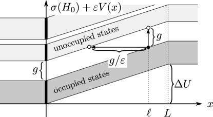
Figure 1: Transitions from the occupied bands into the unoccupied bands are strongly suppressed: To make a transition into an unoccupied state, an electron in the occupied band (black dot) must either overcome the energy gap $g$ (vertical arrow) or tunnel a distance of order $g/\varepsilon$ (horizontal arrow).

If one applies a voltage $\Delta U$ over a distance $L$ modeled by the addition of a potential $V_{\Delta U,L}(x)=\frac{\Delta U}{L}\left(x\chi_{[0,L]}(x)+L\chi_{[L,\infty)}(x)\right)$, then for $\Delta U>g$ the perturbed Hamiltonian will no longer have a spectral gap at $\mu$. Still, the local field strength $\varepsilon:=\frac{\Delta U}{L}$ in the region $[0,L]$ is small if $L$ is a macroscopic distance. For an electron in the Fermi sea that is localized in a microscopic region around the point $\ell\in[0,L]$ the addition of the potential might result in a substantial shift $\varepsilon\ell$ in energy, but it still experiences a small force of order $\varepsilon$. And in order to make a transition into an unoccupied state, it still needs to either overcome the energy gap of size $g$, or tunnel a large distance of order $g/\varepsilon$, see Figure 1. Thus, as long as $g/\varepsilon$ is large, the state $\rho_{0}$ is still an almost-stationary state for the perturbed Hamiltonian $H_{\varepsilon}=H_{0}+V_{\Delta U,L}$. However, $\rho_{0}$ is certainly neither close to the ground state nor to any other type of equilibrium state of $H_{\varepsilon}$. Note that this heuristic picture still remains valid when local interactions between the electrons are taken into account.

At this point let us briefly mention the analogy to shape resonances in the case of finite systems. As the simplest example consider the hydrogen atom in a constant electric field, i.e. the Stark Hamiltonian. No matter how small the electric field is, the spectrum of the Stark Hamiltonian is the whole real line. However, when the field is of order $0<|\varepsilon|\ll 1$, then the ground state of the hydrogen Hamiltonian is close to a shape resonance of the Stark Hamiltonian that is stable for very long times. And when one adiabatically turns on a small electric field, one expects the initial ground state of a hydrogen atom to adiabatically evolve into this resonance. Note that adiabatic theorems for resonances have been established e.g. in [1, 20], although for technical reasons they do not cover the case of the Stark Hamiltonian.

The situation described above for extended non-interacting periodic systems is very similar: instead of a simple ground state the unperturbed state $\rho_{0}$ is the spectral projection of $H_{0}$ onto an infinite dimensional spectral subspace separated by a gap from the rest of the spectrum. And the NEASS described above could be seen as an infinite dimensional resonance for $H_{\varepsilon}$. For interacting extended systems, the analogy is even stronger, as $\rho_{0}$ is indeed the gapped ground state of $H_{0}$ and the corresponding NEASS could also be called a resonance of $H_{\varepsilon}$.

Thus, in order to prove Kubo’s formula also for perturbations that close the spectral gap, one needs to first understand the NEASSs (or “resonances”) of $H_{\varepsilon}$ described above, and then to prove an adiabatic type theorem for NEASSs. This was done in [51], and in Section 3 corresponding results in the thermodynamic limit are discussed.

2.2.2 Justifying Kubo’s formula: Mathematical results

The first work concerned with a rigorous justification of Kubo’s formula in the sense just described, and that we know of, is by Elgart and Schlein [21]. They consider non-interacting electrons on $\mathbb{R}^{2}$ described by the Landau Hamiltonian with smooth and bounded potential and the Fermi energy in a gap of the Hamiltonian. They derive Kubo’s formula for what is often referred to as conductance in this context by proving an appropriate adiabatic theorem. Note that for computing the conductance, one applies the electric field and measures the current only locally, i.e. one replaces $X_{i}$ and $X_{j}$ in our discussion of conductivity above by $G(X_{i})$ and $G(X_{j})$, where $G:\mathbb{R}\to[0,1]$ is a smooth step function with compactly supported derivative $G^{\prime}$. This results in two technical simplifications: no notion of trace per unit volume is needed, and the perturbation is bounded and therefore the gap remains open for $\varepsilon$ sufficiently small. Thus in [21] the standard adiabatic expansion with open gap can be applied and the main technical challenge is to prove the propagation estimates needed for controlling the error in local trace norms (see also [36]). It is also worthwhile to mention that in [21] the adiabatic parameter $\eta$ and the perturbation parameter $\varepsilon$ are identified, $\eta=\varepsilon$, i.e.  the adiabatic limit and the small field limit are taken simultaneously. In [38] we prove Kubo’s formula for the Hall conductivity for gapped magnetic Schrödinger Hamiltonians using the NEASS approach. This requires to deal with the fact that the domain of $H_{\varepsilon}(t)=H_{0}+\varepsilon f(\eta t)X_{j}$ changes at time $t=-1/\eta$ and to prove propagation estimates for time-dependent Stark-type Hamiltonians.

A breakthrough for interacting lattice systems was recently achieved by Bachmann, De Roeck, and Fraas [8]. They prove the first adiabatic theorem for extended lattice systems with local interactions that yields error estimates in local trace norms uniformly in the size of the system. This uniformity was the main mathematical challenge and the main innovation. Their proof exploits locality of interactions in the form of Lieb-Robinson propagation bounds [35] and the local inverse of the Liouvillian introduced by Hastings and Wen [28] (see also [9]). However, Bachmann et al.  [8] require the spectral gap not only for $H_{0}$, but also for the perturbed Hamiltonians $H_{\varepsilon}(t)$. In order to apply their result to slowly varying potential perturbations that close the spectral gap (small fields over large regions), one needs to use the alternative gauge with a time-dependent vector potential and consider the adiabatic response instead, i.e. the first order deviation from ideal adiabatic behavior. This could be done using the results of [39], which are a slight generalization of [8] in several directions: a super-adiabatic version of the theorem is formulated and proved which covers also the trace per unit-volume of extensive observables. This version is then used to derive Kubo’s formula for conductance and conductivity not from adiabatic switching of a small potential, but as the adiabatic response for a Hamiltonian with time-dependent fluxes.

Finally, in [51] an adiabatic theorem for NEASSs in the setting of lattice systems with local interactions was established. It is shown that for perturbations by slowly varying potentials and/or by small local terms the above heuristics for NEASSs can be implemented rigorously by combining the techniques developed in [8] with earlier ideas from space-adiabatic perturbation theory [46]. In the second part of this paper we show how to lift some results from [51] to infinite systems by taking a thermodynamic limit.

2.3 Related results

We end our review on linear response for gapped Hamiltonian systems by briefly mentioning a few related results that did not easily fit into the previous categorization.

In a series of works Bru and de Siqueira Pedra (see [14] and references therein) set up linear response theory and show how to evaluate Kubo’s formula for interacting systems on the lattice in the thermodynamic limit. They do this on a very general level without taking an adiabatic limit and without any kind of gap assumption. Among many other results, they show (2.3) with an error that is $o(\varepsilon)$ uniformly in the system size. The general tools they developed for controlling the thermodynamic limit of interacting systems turn out to be very useful also for the problem discussed in the upcoming section, namely for the construction of NEASS in the thermodynamic limit.

Linear response theory for (open) quantum systems from a general perspective of quantum dynamical systems, discussing in particular also further consequences like Onsager relations, has been worked out by Jaksic, Pillet and collaborators in a series of works. Since we are not aware of a review paper on this topic, we just mention [30], which is probably closest to the setting of the present paper.

There are clearly also physically relevant perturbations that do not (or are not expected to) close the spectral gap of a gapped Hamiltonian, most notably, perturbations by small constant magnetic fields. The corresponding response coefficient is the magnetization. As pointed out before, in this case the response coefficients can be determined from a family of equilibrium states $\rho_{\varepsilon}$ for the family of perturbed Hamiltonians $H_{\varepsilon}$, and one obtains $\sigma_{A}=\frac{\mathrm{d}}{\mathrm{d}\varepsilon}\langle A\rangle_{\rho_{\varepsilon}}\big{|}_{\varepsilon=0}$ by taking a derivative of a family of equilibrium expectation values. For perturbations by constant magnetic fields proving existence of and evaluating this derivative is still a highly non-trivial problem, since such perturbations are not within the realm of regular perturbation theory. Instead, a suitable magnetic perturbation theory was developed by Cornean and Nenciu [16] and applied, for example, in [13] to derive and compute magnetic response coefficients in gapped non-interacting periodic systems. For mobility gapped systems on the lattice, magnetic response was considered also in [47]. We are not aware of any adiabatic theorem applicable to the adiabatic switching of a time-dependent constant magnetic field, even in the gapped case.

Let us finally mention Streda’s formula from [50]. Streda argued that in two dimensional systems the Hall conductivity equals the magnetic response for the particle density, i.e. $\sigma_{12}=\frac{\mathrm{d}}{\mathrm{d}B}\,\tau(\rho_{B})\big{|}_{B=0}$ in infinite non-interacting systems. Bellissard [10] showed that for discrete mobility gapped systems this definition gives the same value as the double-commutator formula, see also [47]. For unbounded Bloch-Landau Hamiltonians, Streda’s formula was recently proved by Cornean, Monaco, and Moscolari [15], see also [17]. We are not aware of similar results on magnetic response for interacting systems.

3 Linear response for interacting fermions in the thermodynamic limit

In this section we show how the results of [51] on the justification of Kubo’s formula using NEASSs for finite gapped systems at zero temperature can be lifted to infinite systems in the thermodynamic limit. It turns out that under suitable assumptions the NEASS $\Pi_{\varepsilon}$ discussed in the previous section exists also as a state on the algebra $\mathcal{A}_{\Gamma}$ of quasi-local observables for the infinite system and that $\Pi_{\varepsilon}$ is automorphically equivalent to the ground state $\rho_{0}$ of the unperturbed Hamiltonian $H_{0}$. Moreover, an adiabatic theorem that allows to formulate and prove Kubo’s formula for the infinite system holds as well. To avoid technicalities, and because of limited space, we report here only the results for the special case of Hamiltonians of the form $H_{\varepsilon}(t)=H_{0}+\varepsilon f(t)V$ and omit the proofs. The general statements and their proofs will be reported elsewhere [29]. There we use results for controlling the thermodynamic limit that were worked out only quite recently in [14, 41].

3.1 Fermions on the lattice: the mathematical framework

We consider fermions with $s\in\mathbb{N}$ internal degrees of freedom (which could be the spin) on the lattice $\Gamma:=\mathbb{Z}^{d}$. Let $\mathcal{P}_{0}(\Gamma)=\set{X\subset\Gamma:}{X|<\infty}$ denote the set of finite subsets of $\Gamma$. Then, for each $X\in\mathcal{P}_{0}(\Gamma)$, the corresponding one-particle Hilbert space is $\mathfrak{h}_{X}:=\ell^{2}(X,\mathbb{C}^{s})$, the $N$-particle Hilbert space is its $N$-fold anti-symmetric tensor product ${\mathfrak{H}}_{X,N}:=\bigwedge_{j=1}^{N}\mathfrak{h}_{X}$, and the fermionic Fock space is $\mathfrak{F}_{X}:=\bigoplus_{N=0}^{s|X|}{\mathfrak{H}}_{X,N}$, where ${\mathfrak{H}}_{X,0}:=\mathbb{C}$. All these Hilbert spaces are finite-dimensional and thus all linear operators on them are bounded. The local $C^{*}$-algebras $\mathcal{A}_{X}=\mathcal{L}(\mathfrak{F}_{X})$ are generated by the identity element $\mathbf{1}_{X}$ and the creation and annihilation operators $a_{x,i}^{*},a_{x,i}$ for $x\in X$ and $1\leq i\leq s$, which satisfy the canonical anti-commutation relations (CAR), i.e.

$$\{a_{x,i},a_{y,j}\}=\{a_{x,i}^{*},a_{y,j}^{*}\}=0,\quad\{a_{x,i},a_{y,j}^{*}\}=\delta_{x,y}\delta_{i,j}\mathbf{1}_{X}\quad\forall x,y\in X,\,1\leq i,j\leq s\,.$$

Here, $\{A,B\}=AB+BA$ denotes the anti-commutator of $A$ and $B$. If we have $X\subset X^{\prime}$, $\mathcal{A}_{X}$ is naturally embedded as a sub-algebra of $\mathcal{A}_{X^{\prime}}$. We denote by $\mathcal{A}_{X}^{N}\subset\mathcal{A}_{X}$ the sub-algebra of elements commuting with the number operator $N_{X}=\sum_{x\in X}a_{x}^{*}a_{x}:=\sum_{x\in X}\sum_{i=1}^{s}a_{x,i}^{*}a_{x,i}$. As elements of $\mathcal{A}_{X}^{N}$ contain even numbers of creation and annihilation operators, it holds that $[\mathcal{A}_{X}^{N},\mathcal{A}_{X^{\prime}}^{N}]=\{0\}$ whenever $X\cap X^{\prime}=\emptyset$. For the infinite system, the local $C^{*}$-algebra is defined by the inductive limit

$$\mathcal{A}_{\Gamma}^{\rm loc}:=\bigcup_{X\in\mathcal{P}_{0}(\Gamma)}\mathcal{A}_{X}\qquad\mbox{and its closure is denoted by}\qquad\mathcal{A}_{\Gamma}:=\overline{\mathcal{A}_{\Gamma}^{\rm loc}}^{\|\cdot\|}\,.$$

In order to define families of operators that are sums of local terms, one uses the concept of “interactions”. In the following we consider sequences of Hamiltonians defined on domains of the form $\Lambda(k)=\set{-k,...,+k}^{d}$ with $k\in\mathbb{N}$. A corresponding interaction $\Phi=\set{\Phi^{\Lambda(k)}}_{k\in\mathbb{N}}$ for a fermionic system on the lattice $\Gamma$ is defined as a family of maps

$$\Phi^{\Lambda(k)}:\set{X\subset\Lambda(k)}\to\mathcal{A}_{\Lambda(k)}^{N}\,,\quad X\mapsto\Phi^{\Lambda(k)}(X)\in\mathcal{A}_{X}^{N}\subset\mathcal{A}_{\Lambda(k)}^{N}$$

with values in the self-adjoint operators. The advantage of considering different maps $\Phi^{\Lambda(k)}$ for different $k\in\mathbb{N}$ instead of restrictions $\Phi|_{\Lambda(k)}$ of a single map $\Phi:\mathcal{P}_{0}(\Gamma)\to\mathcal{A}_{\Gamma}^{\rm loc}$ is the possibility to implement boundary conditions in order to model discrete tube or torus geometries. For example, a hopping term $a^{*}_{(k_{1},\bar{x})}a_{(-k_{1},\bar{x})}$ might only appear in the interaction for the Hamiltonian for that specific value of $k$ in order to connect opposite points on the boundary of $\Lambda(k)$. Moreover, we will also allow for different metrics $d^{\Lambda(k)}(\cdot,\cdot)$ on each $\Lambda(k)$ depending on the intended geometry. For example, for a torus geometry opposite points on the boundary of $\Lambda(k)$ are considered neighbors and their distance is set to one, while for a cube geometry their distance is $2k$.

The associated family of self-adjoint operators $A=\{A^{\Lambda(k)}\}_{k\in\mathbb{N}_{0}}$ corresponding to an interaction $\Phi$ is defined by

$$A^{\Lambda(k)}=A^{\Lambda(k)}(\Phi)=\sum_{X\subset\Lambda(k)}\Phi^{\Lambda(k)}(X)\in\mathcal{A}_{\Lambda(k)}^{N}.$$

We will consider Hamiltonians $H_{0}$ that are operator-families given by interactions $\Phi_{H_{0}}$ that are exponentially localized in the following sense: We say that an interaction is exponentially localized with rate $a>0$, if for all $n\in\mathbb{N}$

$$\sup_{k\in\mathbb{N}}\|\Phi^{\Lambda(k)}\|_{a,n}:=\sup_{k\in\mathbb{N}}\sup_{x,y\in\Gamma}\sum_{\begin{subarray}{c}X\in\mathcal{P}_{0}(\Gamma):\\ x,y\in X\end{subarray}}\mbox{$\Lambda(k)$-diam}(X)^{n}\exp(a\cdot{d^{\Lambda(k)}(x,y)})\,\|\Phi^{\Lambda(k)}(X)\|<\infty\,.$$

In this definition we used implicitly that for any interaction $\Phi$ the maps $\Phi^{\Lambda(k)}$ can be extended to maps on all of $\mathcal{P}_{0}(\Gamma)$ by declaring $\Phi^{\Lambda(k)}(X)=0$, whenever $X\cap(\Gamma\setminus\Lambda(k))\neq\emptyset$. This new mapping is called the extension of $\Phi^{\Lambda(k)}$ and is denoted by the same symbol. Similarly, given $\Phi^{\Lambda(k)}$ and $\Lambda(l)\subset\Lambda(k)$, we define the restriction $\Phi^{\Lambda(k)}|_{\Lambda(l)}:\set{X\subset\Lambda(l)}\to\mathcal{A}_{\Lambda(l)}^{N}$ by

$$\Phi^{\Lambda(k)}|_{\Lambda(l)}(X)=\Phi^{\Lambda(k)}(X)\qquad\forall X\subset\Lambda(l).$$

For the perturbation $V$ we will consider families of potentials $v=\set{v^{\Lambda(k)}:\Lambda(k)\to\mathbb{R}}_{k\in\mathbb{N}}$ that satisfy a uniform Lipschitz condition of the following type,

$$C_{v}:=\sup_{k\in\mathbb{N}}\sup_{x,y\in\Lambda(k)}\frac{|v^{\Lambda(k)}(x)-v^{\Lambda(k)}(y)|}{d^{\Lambda(k)}(x,y)}<\infty\,,$$

and call them for short Lipschitz potentials. With such a potential $v$ we associate the corresponding operator-family $V_{v}=\set{V_{v}^{\Lambda(k)}}_{k\in\mathbb{N}}$ defined by $V_{v}^{\Lambda(k)}=\sum_{x\in\Lambda(k)}v^{\Lambda(k)}(x)a^{*}_{x}a_{x}$. Since in our definitions the functions $\Phi^{\Lambda(k)}$ resp. $v^{\Lambda(k)}$ defining an interaction resp. a potential can be, in principle, completely independent for different domains $\Lambda(k)$, we need to impose additional assumptions in order to guarantee the existence of a thermodynamic limit for all objects appearing in our construction.

Definition 3.1.

1. An exponentially localized interaction $\Phi=\set{\Phi^{\Lambda(k)}}_{k\in\mathbb{N}}$ is said to have a thermodynamic limit if it satisfies the following Cauchy-property:

   $$\forall n\in\mathbb{N}\;\;\exists M_{0}\in\mathbb{N}\;\;\forall M\geq M_{0}\;\;\forall\delta>0\;\;\exists K\geq M\;\;\forall l,k\geq K:\,\left\|\left(\Phi^{\Lambda(l)}-\Phi^{\Lambda(k)}\right)\big{|}_{\Lambda(M)}\right\|_{a,n}\leq\delta\,.$$

   A family of operators is said to have a thermodynamic limit if and only if the corresponding interaction does.

2. A Lipschitz potential $v=\set{v^{\Lambda(k)}}_{k\in\mathbb{N}}$ is said to have a thermodynamic limit if it is locally eventually independent of $k$, i.e. if

   $$\forall M\in\mathbb{N}\;\;\exists K\geq M\;\;\forall l,k\geq K:\,v^{\Lambda(l)}|_{\Lambda(M)}=v^{\Lambda(k)}|_{\Lambda(M)}.$$

For a potential $v$ that has a thermodynamic limit, the point-wise limits $v^{\Lambda(k)}(x)\xrightarrow{k\to\infty}v^{\infty}(x)$ exist for all $x\in\Gamma$ and the limiting function $v^{\infty}$ carries all important information about the potential as far as the thermodynamic limit is concerned.

A relevant example for a Hamiltonian $H_{0}$ that is exponentially localized and has a thermodynamic limit is

$$H^{\Lambda}_{0}=\sum_{(x,y)\in\Lambda^{2}}a^{*}_{x}\,T(x\mathrel{\vbox{\offinterlineskip\halign{\hfil#\hfil\cr$\scriptscriptstyle\Lambda$\cr\kern-0.86108pt\cr$-$\cr}}}y)\,a_{y}+\sum_{x\in\Lambda}a^{*}_{x}\phi(x)a_{x}+\sum_{\{x,y\}\subset\Lambda}a^{*}_{x}a_{x}\,W(d^{\Lambda}(x,y))\,a^{*}_{y}a_{y}-\mu\,N_{\Lambda}\,.$$ (3.1)

Here we assume that the kinetic term $T:\Gamma\to\mathcal{L}(\mathbb{C}^{s})$ is an exponentially fast decaying function with $T(-x)=T(x)^{*}$, the potential term $\phi:\Gamma\to\mathcal{L}(\mathbb{C}^{s})$ is a bounded function taking values in the self-adjoint matrices, and the two-body interaction $W:[0,\infty)\to\mathcal{L}(\mathbb{C}^{s})$ is exponentially decaying and also takes values in the self-adjoint matrices. Note that $x\mathrel{\vbox{\offinterlineskip\halign{\hfil#\hfil\cr$\scriptscriptstyle\Lambda$\cr\kern-0.86108pt\cr$-$\cr}}}y$ in the kinetic term in (3.1) refers to the difference modulo $\Lambda(k)$ if $\Lambda(k)$ is supposed to have a torus geometry.

The most relevant Lipschitz potentials we have in mind are the linear potential $v^{\Lambda(k)}_{D}(x):=x_{i}$ for some $i\in\{1,\ldots,d\}$ if the metrics $d^{\Lambda(k)}$ correspond to a cube geometry (think of Dirichlet boundary conditions on the box) or the saw-tooth potential

$$v^{\Lambda(k)}_{P}(x):=\left\{\begin{array}[]{cl}x_{i}&\mbox{if $x_{i}\in[-\frac{k}{2},\frac{k}{2}]$}\\ k-x_{i}&\mbox{if $x_{i}\in(\frac{k}{2},k]$}\\ -k-x_{i}&\mbox{if $x_{i}\in[-k,-\frac{k}{2})$}\end{array}\right.$$

for the torus geometry. Note that $C_{v_{D}}=C_{v_{P}}=1$ and that both potentials have a thermodynamic limit and converge point-wise to the same function $v^{\infty}(x)=x_{i}$. As we will see, they also define the same response coefficients in the thermodynamic limit when added to a gapped Hamiltonian of the type (3.1).

The following proposition can be proved exactly as Theorem 3.5 in [41] using also Theorem 3.4 and Theorem 3.8 from the same reference. It shows, that the property of having a thermodynamic limit for the interaction resp. the potential guarantees also the existence of a thermodynamic limit for the associated evolution operators.

Proposition 3.1.

Thermodynamic limit of Cauchy-interactions [41]
Let $H_{0}$ and $H_{1}$ be operator-families that are associated with two exponentially localized interactions and let $v$ be a Lipschitz potential with associated operator-family $V_{v}$, all having a thermodynamic limit. Let $V:=V_{v}+H_{1}$.

1. Let $H_{\varepsilon}:=H_{0}+\varepsilon V$ for some $\varepsilon\in\mathbb{R}$. Then there exists a unique one-parameter group $t\mapsto{\mathrm{e}}^{\mathrm{i}\mathcal{L}_{H_{\varepsilon}}t}:\mathcal{A}_{\Gamma}\to\mathcal{A}_{\Gamma}$ of automorphisms such that for all $A\in\mathcal{A}_{\Gamma}^{\rm loc}$

   $${\mathrm{e}}^{\mathrm{i}\mathcal{L}_{H_{\varepsilon}}t}[A]=\lim_{k\to\infty}{\mathrm{e}}^{\mathrm{i}H_{\varepsilon}^{\Lambda(k)}t}\,A\,{\mathrm{e}}^{-\mathrm{i}H_{\varepsilon}^{\Lambda(k)}t}$$

2. Let $f:\mathbb{R}\to\mathbb{R}$ be smooth and put $H_{\varepsilon,\eta}(t):=H_{0}+\varepsilon f(\eta t)V$ for some $\varepsilon\in\mathbb{R}$. Denote by $U^{\Lambda(k),\eta}(t,t_{0})$ the evolution family generated by $H_{\varepsilon,\eta}(t)$, i.e. the solution to the Schrödinger equation

   $$\mathrm{i}\tfrac{\mathrm{d}}{\mathrm{d}t}U^{\Lambda(k),\eta}(t,t_{0})=H_{\varepsilon,\eta}^{\Lambda(k)}(t)\,U^{\Lambda(k),\eta}(t,t_{0})\qquad\mbox{with }\quad U^{\Lambda(k),\eta}(t_{0},t_{0})={\rm Id}\,.$$

   Then there exists a unique co-cycle of automorphisms $\mathfrak{U}^{\eta}_{t,t_{0}}:\mathcal{A}_{\Gamma}\to\mathcal{A}_{\Gamma}$ such that for all $A\in\mathcal{A}_{\Gamma}^{\rm loc}$

   $$\mathfrak{U}^{\eta}_{t,t_{0}}[A]=\lim_{k\to\infty}U^{\Lambda(k),\eta}(t,t_{0})^{*}\,A\,U^{\Lambda(k),\eta}(t,t_{0})\,.$$

The main additional assumption on the Hamiltonian $H_{0}$ that we need is the gap assumption: We say that the operator-family $H_{0}=\{H_{0}^{\Lambda(k)}\}_{k\in\mathbb{N}}$ has a simple gapped ground state, if there exists $L\in\mathbb{N}$ such that for all $k\geq L$ and corresponding $\Lambda(k)$ the smallest eigenvalue $E_{0}^{\Lambda(k)}$ of the operator $H_{0}^{\Lambda(k)}$ is simple and the spectral gap is uniform in the system size, i.e. there exists $g>0$ such dist$(E_{0}^{\Lambda(k)},\sigma(H_{0}^{\Lambda(k)})\setminus\{E_{0}^{\Lambda(k)}\})\geq g>0$ for all $k\geq L$.

In addition, we require that also the sequence of ground states $\rho_{0}^{\Lambda(k)}$ has a thermodynamic limit. To formulate this condition, recall that a normalized positive linear functional $\omega$ on the $C^{*}$-algebra $\mathcal{A}_{\Gamma}$ is called a state. Here normalized means $\omega({\rm id})=1$ and positive means $\omega(A^{*}A)\geq 0$ for all $A\in\mathcal{A}_{\Gamma}$. By the Banach-Alaoglu theorem, the set of states $E_{\mathcal{A}_{\Gamma}}$ is weak^∗-compact. If $\mathcal{B}$ is a subalgebra of $\mathcal{A}_{\Gamma}$ and $\omega$ is a state on $\mathcal{B}$, then there exists a state $\hat{\omega}$ on $\mathcal{A}_{\Gamma}$ which extends $\omega$ by the Hahn-Banach theorem. In this way, the states $B\mapsto{\mathrm{tr}}(\rho_{0}^{\Lambda(k)}B)$ can be extended to the whole algebra $\mathcal{A}_{\Gamma}$ and are denoted by the same symbol $\rho_{0}^{\Lambda(k)}$. To avoid the extraction of subsequences, we will assume that the sequence of ground states $(\rho_{0}^{\Lambda(k)})_{k\in\mathbb{N}}$ converges to a unique limiting point $\rho_{0}\in E_{\mathcal{A}_{\Gamma}}$.

(A1) Assumptions on $H_{0}$.
Let $H_{0}$ be the Hamiltonian of an exponentially localized interaction that has a thermodynamic limit. We assume that $H_{0}$ has a gapped ground state such that the sequence of ground states $(\rho_{0}^{\Lambda(k)})_{k\in\mathbb{N}_{0}}$ converges in the weak^∗-topology to a state $\rho_{0}$ on $\mathcal{A}_{\Gamma}$.

(A2) Assumptions on the perturbation.
Let $V=V_{v}+H_{1}$, where $v$ is a Lipschitz potential and $V_{v}$ denotes the corresponding operator-family, and $H_{1}$ is the Hamiltonian of an exponentially localized interaction, both having a thermodynamic limit.

Note that for non-interacting Hamiltonians $H_{0}$ of the type (3.1) on a torus, i.e.  with $W\equiv 0$, condition (A1) is satisfied whenever the chemical potential $\mu$ lies in a gap of the spectrum of the corresponding one-body Hamiltonian operator on the infinite domain, a condition that can be checked easily. And it was recently shown in [26, 19], that for sufficiently small $W\not=0$ the spectral gap remains open.

We have now all prerequisites to formulate our main results on the existence and properties of NEASS for interacting systems in the thermodynamic limit. They are all adaptions of corresponding results for finite systems proved in [51]. As they are not simple corollaries of [51] but require some careful adaptions, their proofs will be given elsewhere [29].

The first theorem states that under Assumptions (A1) and (A2) there exists a NEASS for the perturbed Hamiltonian $H_{\varepsilon}=H_{0}+\varepsilon V$ close to the ground state of $H_{0}$ (cf. Theorem 3.1 in [51]).

Theorem 3.1.

Existence of NEASSs
Let the Hamiltonian $H_{\varepsilon}=H_{0}+\varepsilon V$ satisfy (A1) and (A2). Then for any $\varepsilon\in[-1,1]$ there exists a near-identity automorphism $\alpha_{\varepsilon}$ of $\mathcal{A}_{\Gamma}$ such that the state $\Pi_{\varepsilon}$ defined by

$$\Pi_{\varepsilon}(A):=\rho_{0}(\alpha_{\varepsilon}[A])\qquad\mbox{for all }A\in\mathcal{A}_{\Gamma}$$

is almost-invariant in the following sense: for any $n\in\mathbb{N}$ there exists a constant $C_{n}>0$ such that for all finite $X\subset\Gamma$, $A\in\mathcal{A}_{X}^{N}\subset\mathcal{A}_{\Gamma}$, and $\varepsilon\in[-1,1]$

$$\left|\Pi_{\varepsilon}({\mathrm{e}}^{\mathrm{i}\mathcal{L}_{H_{\varepsilon}}t}[A])-\Pi_{\varepsilon}(A)\right|\leq C_{n}\,{|\varepsilon|^{n}}(1+|t|^{2d})\,|X|^{3}\,\|A\|\,.$$ (3.2)

By near-identity we mean that $\alpha_{\varepsilon}$ is of the form $\alpha_{\varepsilon}={\mathrm{e}}^{\mathrm{i}\varepsilon\mathcal{L}_{S_{\varepsilon}}}$ for an almost exponentially localized operator family $S_{\varepsilon}$ that has a thermodynamic limit.

The next theorem is a special case of a more general adiabatic theorem for NEASS, cf. Theorem 5.1 in [51]. It shows that when adiabatically switching on the perturbation, then the initial ground state of $H_{0}$ dynamically evolves up to small errors into the corresponding NEASS $\Pi_{\varepsilon}$ for the perturbed Hamiltonian $H_{\varepsilon}$ as long as the adiabatic parameter $\eta$ is small but not too small (see also Proposition 3.2 in [51]).

Theorem 3.2.

Adiabatic switching
Let the Hamiltonian $H_{\varepsilon}=H_{0}+\varepsilon V$ satisfy (A1) and (A2). Let $f:\mathbb{R}\to\mathbb{R}$ be a smooth “switching” function with $f(t)=0$ for $t\leq-1$ and $f(t)=1$ for $t\geq 0$, and define $H_{\varepsilon,\eta}(t):=H_{0}+\varepsilon f(\eta t)V$. Let $\mathfrak{U}^{\eta}_{t,t_{0}}$ be the Heisenberg time-evolution on $\mathcal{A}_{\Gamma}$ generated by $H_{\varepsilon,\eta}(t)$ with adiabatic parameter $\eta\in(0,1]$.

Then for any $n>d$ there exists a constant $C_{n}$ such that for any finite $X\subset\Gamma$ and $A\in\mathcal{A}_{X}^{N}\subset\mathcal{A}_{\Gamma}$ and for all $t\geq 0$

$$\left|\rho_{0}(\mathfrak{U}^{\eta}_{t/\eta,-1/\eta}[A])-\Pi_{\varepsilon}(A)\right|\leq\;\frac{|\varepsilon|^{n+1}+\eta^{n+1}}{\eta^{d+1}}\,C_{n}\,(1+t^{d+1})\,|X|^{2}\,\|A\|\,,$$ (3.3)

where $\Pi_{\varepsilon}$ is the NEASS of $H_{\varepsilon}$ constructed in Theorem 3.1.

Note that (3.3) shows that, as long as the adiabatic parameter $\eta$ satisfies $1\gg\eta\gg|\varepsilon|^{\frac{n+1}{d+1}}$ for some $n>d$, the initial ground state $\rho_{0}$ of $H_{0}$ evolves, up to a small error, into the NEASS $\Pi_{\varepsilon}$ that is independent of the form of the switching function $f$ and of $\eta$. Slower switching must be excluded, because, in general, the NEASS is an almost-invariant but not an invariant state for the instantaneous Hamiltonian. Its life-time depends on the strength of the perturbation, i.e. on $\varepsilon$, and it is thus not surprising that the relevant time scale for the adiabatic switching process depends on $\varepsilon$ as well.

In order to compute response coefficients, we need to expand $\Pi_{\varepsilon}$ in powers of $\varepsilon$ (cf. Proposition 3.1 in [51]).

Proposition 3.2.

Asymptotic expansion of the NEASS
Under the assumptions of Theorem 3.1 there exist linear maps $\mathcal{K}_{j}:\mathcal{A}_{\Gamma}^{\rm loc}\to\mathcal{A}_{\Gamma}$, $j\in\mathbb{N}$, such that for any $n\in\mathbb{N}$ there is a constant $C_{n}$ such that for any finite $X\subset\Gamma$ and $A\in\mathcal{A}_{X}^{N}\subset\mathcal{A}_{\Gamma}$ it holds that

$$\left|\Pi_{\varepsilon}(A)-\sum_{j=0}^{n}\varepsilon^{j}\,\rho_{0}(\mathcal{K}_{j}[A])\right|\;\leq\;C_{n}\,|\varepsilon|^{n+1}\,|X|^{2}\,\|A\|\,.$$

The constant term is $\mathcal{K}_{0}=\mathbf{1}_{\mathcal{A}_{\Gamma}}$, which shows that $\alpha_{\varepsilon}$ is indeed a near-identity automorphism when $|\varepsilon|\ll 1$. The linear term $\mathcal{K}_{1}$ is a densely defined derivation on $\mathcal{A}_{\Gamma}$ that satisfies

$$\rho_{0}(\mathcal{K}_{1}[A]) = -\,\lim_{k\to\infty}\left\langle\left[\mathcal{I}_{H_{0}^{\Lambda(k)}}(V^{\Lambda(k)}),A\right]\right\rangle_{\rho_{0}^{\Lambda(k)}}$$ (3.4)

$$= \lim_{k\to\infty}{\mathrm{tr}}\left(\mathcal{L}_{H_{0}^{\Lambda(k)}}^{-1}([V^{\Lambda(k)},\rho_{0}^{\Lambda(k)}])\,A\right)$$

for every $A\in\mathcal{A}_{\Gamma}^{\rm loc}$. Here $\mathcal{I}_{H_{0}^{\Lambda(k)}}$ is a local version of the inverse Liouvillian introduced in [28] and from the first expression in (3.4) it follows that $\rho_{0}(\mathcal{K}_{1}[A])$ depends on $V_{v}$ only through the limiting function $v^{\infty}$.

Finally, we can combine the previous results in order to formulate our main theorem about linear and higher order response for gapped interacting systems in the thermodynamic limit (cf. Theorem 4.1 in [51]).

Theorem 3.3.

Linear and higher order response
Under the same assumptions as in Theorem 3.2, let again $\mathfrak{U}^{\eta}_{t,t_{0}}$ be the Heisenberg time-evolution on $\mathcal{A}_{\Gamma}$ generated by $H_{\varepsilon,\eta}(t)$ with adiabatic parameter $\eta\in(0,1]$. For $A\in\mathcal{A}_{\Gamma}$ define the total response as

$$\Sigma^{\varepsilon,\eta,f}_{A}(t):=\rho_{0}(\mathfrak{U}^{\eta}_{t/\eta,-1/\eta}[A])-\rho_{0}(A)\,,$$

and for $j\in\mathbb{N}$ the $j$th order response coefficient as $\sigma_{A,j}:=\rho_{0}(\mathcal{K}_{j}[A])$, where the $\mathcal{K}_{j}$’s were defined in Proposition 3.2 and $\sigma_{A,1}$ is explicitly given by (3.4), i.e. by the thermodynamic limit of Kubo’s formula (2.6).

Then for any $n,m\in\mathbb{N}$ there exists a constant $C_{n,m}$ independent of $\varepsilon$, such that for any finite $X\subset\Gamma$ and $A\in\mathcal{A}_{X}^{N}\subset\mathcal{A}_{\Gamma}$ and all $t\geq 0$

$$\sup_{\eta\,\in\left[|\varepsilon|^{m},\,|\varepsilon|^{\frac{1}{m}}\right]}\left|\Sigma^{\varepsilon,\eta,f}_{A}(t)-\sum_{j=1}^{n}\varepsilon^{j}\sigma_{A,j}\right|\leq|\varepsilon|^{n+1}\,C_{n,m}\,(1+t^{d+1})\,|X|^{2}\,\|A\|\,.$$ (3.5)

Note that the condition that $\eta\in[|\varepsilon|^{m},|\varepsilon|^{\frac{1}{m}}]$ for some $m\in\mathbb{N}$ makes sure that the switching is neither too slow ($\eta\geq|\varepsilon|^{m}$) nor too fast ($\eta\leq|\varepsilon|^{\frac{1}{m}}$). Too slow switching would be switching on time-scales longer than the life-time of the NEASS, while too fast switching would no longer allow for an expansion of the total response in powers of $\varepsilon$.

While we believe that this result and the NEASS approach in general are an important contribution to the mathematical understanding of linear response theory for transport in gapped Hamiltonian systems, there are still several open questions: An obvious conjecture would be that our results remain valid if one replaces the gap condition for the local Hamiltonians in Assumption (A1) by a gap condition for the Hamiltonian for the infinite system (in the GNS representation). At least for the case that $V\in\mathcal{A}_{\Gamma}$, we expect that the methods recently developed in [40] can be used to adapt our proofs accordingly.

A presumably much harder but physically more interesting problem is to justify Kubo’s formula for current response in situations where $H_{0}$ no longer has a spectral gap but only a mobility gap. Even for non-interacting systems we know of no results in this direction yet.

References

- [1] W. Abou Salem and J. Fröhlich: Adiabatic theorem for quantum resonances. Comm. Math. Phys. 273:651–675 (2007).
- [2] M. Aizenman and G.-M. Graf: Localization bounds for an electron gas. Journal of Physics A: Mathematical and General 31:6783 (1998).
- [3] G. Androulakis, J. Bellissard, and C. Sadel: Dissipative dynamics in semiconductors at low temperature. Journal of Statistical Physics 147:448–486 (2012).
- [4] J. Avron: Why is the Hall conductance quantized? Solution of an open math-phys problem. Open Problems in Mathematical Physics http://web.math.princeton.edu/~aizenman/OpenProblems_MathPhys/17_Avron.pdf (2017).
- [5] J. Avron and R. Seiler: Quantization of the Hall conductance for general, multiparticle Schrödinger Hamiltonians, Phys. Rev. Lett. 54: 259–262 (1985).
- [6] J. Avron, R. Seiler, and B. Simon: Homotopy and quantization in condensed matter physics, Phys. Rev. Lett. 51: 51–53 (1983).
- [7] S. Bachmann, A. Bols, W. De Roeck, and M. Fraas: A many-body index for quantum charge transport. Comm. Math. Phys. Online First (2019).
- [8] S. Bachmann, W. De Roeck, and M. Fraas: The adiabatic theorem and linear response theory for extended quantum systems. Comm. Math. Phys. 361:997–1027 (2018).
- [9] S. Bachmann, S. Michalakis, B. Nachtergaele, and R. Sims: Automorphic equivalence within gapped phases of quantum lattice systems. Comm. Math. Phys. 309:835–871 (2012).
- [10] J. Bellissard: -algebras in solid state physics. 2D electrons in a uniform magnetic field. In Operator Algebras and Application. D.E. Evans and M. Takesaki (1988).
- [11] J. Bellissard, A. van Elst, and H. Schulz-Baldes: The noncommutative geometry of the quantum Hall effect. J. Math. Phys. 35:5373–5451 (1994).
- [12] J. Bouclet, F. Germinet, A. Klein, and J. Schenker: Linear response theory for magnetic Schrödinger operators in disordered media. J. Func. Anal. 226:301–372 (2005).
- [13] P. Briet, H. Cornean, and B. Savoie: A Rigorous Proof of the Landau-Peierls Formula and much more. Ann. H. Poincaré 13:1–40 (2012).
- [14] J.-B. Bru and W. de Siqueira Pedra: Lieb–Robinson Bounds for Multi-Commutators and Applications to Response Theory. Springer Briefs in Math. Phys. 13, Springer (2016).
- [15] H. Cornean, D. Monaco, and M. Moscolari: Beyond diophantine Wannier diagrams: Gap labelling for Bloch-Landau Hamiltonians. arXiv:1810.05623 (2018).
- [16] H. Cornean and G. Nenciu: On eigenfunction decay of two dimensional magnetic Schrödinger operators. Commun. Math. Phys. 192:671–685 (1998).
- [17] H. Cornean, G. Nenciu, and T. Pedersen: The Faraday effect revisited: General theory. J. Math. Phys. 47:013511 (2006).
- [18] G. De Nittis and M. Lein: Linear Response Theory: An Analytic-Algebraic Approach. Springer Briefs in Mathematical Physics Vol. 21, Springer (2017).
- [19] W. De Roeck and M. Salmhofer: Persistence of exponential decay and spectral gaps for interacting fermions. Comm. Math. Phys. , Online First (2018).
- [20] A. Elgart and G. Hagedorn: An adiabatic theorem for resonances. Commun. Pure Appl. Math. 64:1029-1058 (2011).
- [21] A. Elgart and B. Schlein: Adiabatic charge transport and the Kubo formula for Landau-type Hamiltonians. Commun. Pure Appl. Math. Math. 57:590–615 (2004).
- [22] J. Fröhlich: Chiral anomaly, topological field theory, and novel states of matter. Rev. Math. Phys. 30:1840007 (2018).
- [23] J. Fröhlich and T. Kerler: Universality in quantum Hall systems. Nucl. Phys. B 354:369–417 (1991).
- [24] A. Giuliani, V. Mastropietro and M. Porta, Universality of the Hall conductivity in interacting electron systems, Comm. Math. Phys. 349:1107–1161 (2017).
- [25] G.M. Graf: Aspects of the integer quantum Hall effect. In Proceedings of Symposia in Pure Mathematics 76: 429, American Mathematical Society (2007).
- [26] M. Hastings: The Stability of Free Fermi Hamiltonians. J. Math. Phys. 60: 042201 (2019).
- [27] M. Hastings and S. Michalakis: Quantization of Hall conductance for interacting electrons on a torus. Comm. Math. Phys. 334:433–471 (2015).
- [28] M. Hastings and X.-G. Wen: Quasiadiabatic continuation of quantum states: The stability of topological ground-state degeneracy and emergent gauge invariance. Phys. Rev. B 72:045141 (2005).
- [29] J. Henheik and S. Teufel. In preparation 2020.
- [30] V. Jaksic, Y. Ogata, and C.-A. Pillet: The Green-Kubo formula for locally interacting open fermionic systems. Ann. Henri Poincaré, 8:1013–1036 (2006).
- [31] T. Kato: On the adiabatic theorem of quantum mechanics. J. Phys. Soc. Jap. 5: 435–439 (1950).
- [32] A. Klein, O. Lenoble, and P. Müller: On Mott’s formula for the ac-conductivity in the Anderson model, Annals of Math. 549–577 (2007).
- [33] R. Kubo: Statistical-mechanical theory of irreversible processes. I. General theory and simple applications to magnetic and conduction problems, J. Phys. Soc. Japan 12:570–586 (1957).
- [34] R. Laughlin: Anomalous Quantum Hall Effect: An Incompressible Quantum Fluid with Fractionally Charged Excitations, Phys. Rev. Lett. 50:1395–1398 (1983).
- [35] E. Lieb and D. Robinson: The finite group velocity of quantum spin systems. Comm. Math. Phys. 28:251–257 (1972).
- [36] G. Marcelli: Improved energy estimates for a class of time-dependent perturbed Hamiltonians. arXiv:1904.11300 (2019).
- [37] G. Marcelli, D. Monaco, G. Panati, and S. Teufel: A new approach to transport coefficients in the quantum (spin) Hall effect. In preparation (2020).
- [38] G. Marcelli and S. Teufel. In preparation (2020).
- [39] D. Monaco and S. Teufel: Adiabatic currents for interacting electrons on a lattice. Rev. Math. Phys. 31:1950009 (2019).
- [40] A. Moon and Y. Ogata: Automorphic equivalence within gapped phases in the bulk. arXiv:1906.05479 (2019).
- [41] B. Nachtergaele, R. Sims, and A. Young: Quasi-locality bounds for quantum lattice systems. I. Lieb-Robinson bounds, quasi-local maps, and spectral flow automorphisms. J. Math. Phys. 60:061101 (2019).
- [42] G. Nenciu: On asymptotic perturbation theory for quantum mechanics: almost invariant subspaces and gauge invariant magnetic perturbation theory. J. Math. Phys. 43:1273–1298 (2002).
- [43] Q. Niu and D.J. Thouless. Quantised adiabatic charge transport in the presence of substrate disorder and many-body interaction. J. Phys. A: Math. Gen. 17:2453–2462 (1984).
- [44] Q. Niu, D.J. Thouless, and Y.-Sh. Wu: Quantized Hall conductance as a topological invariant. Phys. Rev. B 31:3372–3377 (1985).
- [45] G. Panati, H. Spohn, and S. Teufel: Effective dynamics for Bloch electrons: Peierls substitution and beyond. Commun. Math. Phys. 242:547–578 (2003).
- [46] G. Panati, H. Spohn, and S. Teufel: Space-adiabatic perturbation theory. Adv. Theor. Math. Phys. 7:145–204 (2003).
- [47] H. Schulz-Baldes and S. Teufel: Orbital polarization and magnetization for independent particles in disordered media. Comm. Math. Phys. 319:649–681 (2013).
- [48] B. Simon: Holonomy, the quantum adiabatic theorem, and Berry’s phase. Phys. Rev. Lett. 51:2167–2170 (1983).
- [49] B. Simon: Fifteen problems in mathematical physics. Perspectives in Mathematics, Birkhäuser, Basel 423 (1984).
- [50] P. Streda: Theory of quantised Hall conductivity in two dimensions. J. Phys. C 15, L717 (1982).
- [51] S. Teufel: Non-equilibrium almost-stationary states and linear response for gapped quantum systems. Comm. Math. Phys. 373:621–653 (2020).
- [52] S. Teufel: Adiabatic Perturbation Theory in Quantum Dynamics. Lecture Notes in Mathematics 1821, Springer (2003).
- [53] D.J. Thouless, M. Kohmoto, M. Nightingale, and M. den Nijs: Quantized Hall conductance in a two-dimensional periodic potential. Phys. Rev. Lett. 49:405 (1982).