Sharp boundary $\varepsilon$-regularity of optimal transport maps

Abstract.

In this paper we develop a boundary $\varepsilon$-regularity theory for optimal transport maps between bounded open sets with $C^{1,\alpha}$-boundary. Our main result asserts sharp $C^{1,\alpha}$-regularity of transport maps at the boundary in form of a linear estimate under certain assumptions: The main quantitative assumptions are that the local nondimensionalized transport cost is small and that the boundaries are locally almost flat in $C^{1,\alpha}$. Our method is completely variational and builds on the recently developed interior regularity theory.

1. Introduction

Let $d\geq 2$, $\alpha\in(0,1)$, and $\Omega_{0},\Omega_{1}\subset\mathbb{R}^{d}$ be bounded open sets with $C^{1,\alpha}$-boundary. For $\lambda_{0},\lambda_{1}\in[1/2,2]$, let $T$ be a unique solution to the optimal transport problem between constant densities $\lambda_{0}\chi_{\Omega_{0}}$ and $\lambda_{1}\chi_{\Omega_{1}}$ of same mass:

(1.1) $$\min_{T\sharp(\lambda_{0}\chi_{\Omega_{0}})=\lambda_{1}\chi_{\Omega_{1}}}\int_{\mathbb{R}^{d}}|T(x)-x|^{2}\lambda_{0}\chi_{\Omega_{0}}dx,$$

where $\chi_{\Omega_{i}}$ denotes the characteristic function of $\Omega_{i}$ and, with an abuse of notation, $T\sharp(\lambda_{0}\chi_{\Omega_{0}})$ denotes the push-forward by $T$ of the measure $\lambda_{0}\chi_{\Omega_{0}}dx$.

In this paper we aim at clarifying how the regularity of the boundary $\partial\Omega_{i}$ influences boundary regularity of the map $T:\Omega_{0}\to\Omega_{1}$, focusing on the simplest case of constant densities. To this end we develop a boundary $\varepsilon$-regularity theory on the intrinsic $L^{2}$-level, building on the interior $\varepsilon$-regularity theory by the last author and his co-authors [16, 15].

Our main result asserts sharp $C^{1,\alpha}$-regularity of $T$ near the boundary under certain assumptions, which roughly mean that $T$ is quantitatively “close to being the identity” as in usual $\varepsilon$-regularity theory. Besides the main quantitative assumption, we assume two qualitative properties: One is the tangency condition in an open ball $B_{R}(p)\subset\mathbb{R}^{d}$ that

(1.2) $$p\in\partial\Omega_{0}\cap\partial\Omega_{1},\quad\nu_{0}(p)=\nu_{1}(p),\quad\partial\Omega_{i}\cap B_{R}(p)\ \textrm{is connected}\ (i=0,1),$$

where $\nu_{i}$ denotes the outer unit normal of $\partial\Omega_{i}$: The other is the topological condition in $B_{R}(p)$ that

(1.3) $$T(B_{R/2}(p)\cap\Omega_{0})\subset B_{R}(p)\quad\textrm{and}\quad T^{-1}(B_{R/2}(p)\cap\Omega_{1})\subset B_{R}(p),$$

where by abuse of notation we let $T^{-1}$ stand for the optimal transport map from $\lambda_{1}\chi_{\Omega_{1}}$ to $\lambda_{0}\chi_{\Omega_{0}}$ (since $T^{-1}(T(x))=x$ and $T(T^{-1}(y))=y$ hold a.e. [25, Theorem 2.12 (iv)]) and understand that the inclusions hold up to null sets.

Here is our main theorem, which asserts $C^{1,\alpha}$-regularity with a linear estimate:

Theorem 1.1 (Boundary $\varepsilon$-regularity).

There exist constants $\varepsilon,C>0$ depending only on $d,\alpha$ with the following property: Let $p\in\mathbb{R}^{d}$, $R>0$, $\lambda_{0},\lambda_{1}\in[1/2,2]$ and $T$ be the solution of (1.1). If the tangency condition (1.2) and the topological condition (1.3) hold in $B_{R}(p)$, and if

(1.4) $$\varepsilon^{\prime}:={1\over R^{d+2}}\int_{B_{R}(p)}|T-x|^{2}\lambda_{0}\chi_{\Omega_{0}}dx+R^{2\alpha}[\nu_{0}]_{\alpha,B_{R}(p)}^{2}+R^{2\alpha}[\nu_{1}]_{\alpha,B_{R}(p)}^{2}\leq\varepsilon,$$

then $T$ is of class $C^{1,\alpha}$ in $\overline{B_{R/16}(p)\cap\Omega_{0}}$, and we have the estimate

$$R^{2\alpha}[\nabla T]_{\alpha,B_{R/16}(p)}^{2}\leq C\varepsilon^{\prime}.$$

Recall that the corresponding convex potential $u$ (i.e., $\nabla u=T$ a.e.) solves the Monge-Ampère equation in Brenier’s sense (cf. [25, Section 4.1.4]):

(1.5) $$\det(\nabla^{2}u)=\lambda_{0}/\lambda_{1}\quad\text{in }\Omega_{0},\quad\nabla u(\Omega_{0})=\Omega_{1}.$$

Our proof is crucially based on the observation that in a quantitative sense the Monge-Ampère equation may be linearized by a Poisson equation (cf. [25, Exercise 4.1]) with a certain (linearized) Neumann boundary condition on $\partial\Omega_{0}$.

Theorem 1.1, however, highlights that in view of regularity theory there is a significant difference between linear and nonlinear boundary conditions. We first notice that in terms of the potential $u$, Theorem 1.1 asserts $u\in C^{2,\alpha}$ under $\partial\Omega_{i}\in C^{1,\alpha}$. This should be compared with the fact that $\partial\Omega_{i}\in C^{2,\alpha}$ is necessary for $u\in C^{2,\alpha}$ in case of a Neumann boundary condition. We briefly argue how this difference occurs, focusing on $d=2$. Suppose locally that $\partial\Omega_{0}$ and $\partial\Omega_{1}$ coincide (but are different globally), and also the generic behavior that $\nabla u(\partial\Omega_{0})=\partial\Omega_{1}$ (“boundary goes to boundary”). Then the linearized boundary condition should be $\partial u/\partial\nu=0$, that is, $\gamma^{\prime}=(\nabla u\circ\gamma)/|\nabla u\circ\gamma|$ (if $\nabla u\neq 0$), where $\gamma$ denotes the unit speed parametrization of the boundary curve of $\Omega_{0}$; roughly speaking, this is a “1st order = 1st order” relation, so necessarily $\gamma\in C^{2,\alpha}$ if $u\in C^{2,\alpha}$. However, the nonlinear boundary condition $\nabla u(\partial\Omega_{0})=\partial\Omega_{1}$ means that $g(\partial_{1}u(z,g(z)))=\partial_{2}u(z,g(z))$ if $\partial\Omega_{0}$ and $\partial\Omega_{1}$ are locally represented by the graph of $g$; this is a “0th order = 1st order” relation, so just $g\in C^{1,\alpha}$ is required for $u\in C^{2,\alpha}$.

In Theorem 1.1, the topological condition is unremovable in the sense that, without this condition, our $L^{2}$-smallness assumption does not rule out a “separation of boundary layer” as demonstrated in Remark 3.3. This phenomenon represents one essential difference from the interior $\varepsilon$-regularity theory on $L^{2}$-level. The tangency condition on the other hand is not restrictive thanks to the affine invariance of the optimal transportation problem (see Remark 6.2).

Theorem 1.1 generalizes Chen and Figalli’s boundary $\varepsilon$-regularity theory on $L^{\infty}$-level [5, Theorem 2.2] in a certain direction. Their result in particular asserts $C^{1,\alpha^{\prime}}$-regularity of $T$ for some (non-explicit) $\alpha^{\prime}\in(0,1)$ when $\Omega_{i}$, $i=0,1$, are $C^{2}$-domains. Compared to their result, on one hand, our assertion is stronger by giving the (explicit) sharp exponent $\alpha$, and on the other hand, our assumption is not only weaker but also described in a completely local way (see Remark 3.5 for details). We should however clarify that Chen and Figalli’s method can deal with non-quadratic costs (resp. non-constant densities) as small perturbations from the quadratic cost (resp. the constant densities), which are not covered by our result. We are confident that our approach is also applicable to non-constant densities as in [16], and hope that it can be extended to non-quadratic costs, as in [21].

Theorem 1.1 may be also regarded as an extension of Jhaveri’s recent boundary $\varepsilon$-regularity result [17, Theorem 2.6] à la Chen and Figalli, which asserts (lower order) $C^{0,\beta}$-regularity of $T$ for any $\beta\in(0,1)$, only assuming $C^{1,\alpha}$-regularity for domains. In the same paper, Jhaveri gives several sharp counterexamples, in particular showing that for any small $\varepsilon>0$ there are smooth domain $\Omega_{0}$ and $\Omega_{1}$ that are $\varepsilon$-close in $C^{1}$-sense for which the optimal transport map is even discontinuous (in fact, they may be close in $C^{1,\alpha^{\prime}}$-sense for small $\alpha^{\prime}(\varepsilon)$). Our assumption of $C^{1,\alpha}$-boundary regularity is thus sharp for establishing an $\varepsilon$-regularity theory.

The regularity of optimal transport maps is one of the most active area in the study of optimal transportation. Although Brenier’s theorem ensures existence and uniqueness of transport maps between general probability densities $\rho_{0}$ and $\rho_{1}$, their regularity sensitively depends on not only the regularity of $\rho_{i}$ but also the global geometry of ${\rm supp}\rho_{i}$ ($=\overline{\Omega_{i}}$). Concerning the global regularity of $T$ for the quadratic cost, it is shown by Caffarelli [3] that $T\in C^{0,\delta}(\overline{\Omega_{0}})$ for small $\delta>0$ when $\rho_{i}\in L^{\infty}(\Omega_{i})$ is uniformly positive and $\Omega_{i}$ is bounded and convex for $i=0,1$; recently, Savin and Yu [23] strengthen this regularity up to $C^{0,\delta}(\overline{\Omega_{0}})$ for any $\delta\in(0,1)$ in case of $d=2$ and constant densities. Beyond the above lower order regularity, after Delanoë [9] and Urbas [24], Caffarelli [4] also shows that $T\in C^{1,\alpha}(\overline{\Omega_{0}})$ if in addition $0<\rho_{i}\in C^{0,\alpha}(\overline{\Omega_{i}})$ and $\Omega_{i}$ is $C^{2}$ uniformly convex for $i=0,1$. In a recent study, Chen, Liu, and Wang [6] ensure the same assertion even for $C^{1,1}$ convex domains (and small perturbations of them [8]); when $d=2$, they also verify the same result for $C^{1,\alpha}$ convex domains [7]. The convexity assumption is known to be essential for global regularity (see e.g. [2, 18]); in this paper, in view of the local character of an $\varepsilon$-regularity result, we do not restrict our attention to convex domains. Without convexity (or near convexity), the best known approach seems to be obtaining partial regularity of $T$ as developed in [12, 13, 11, 16]. In particular, the latter two studies by de Philippis-Figalli [11] and by Goldman and the last author [16] are straightforward consequences of an interior $\varepsilon$-regularity theory. The aforementioned theory by Chen and Figalli [5] is a boundary counterpart of de Philippis and Figalli’s interior theory, and seems to be a first breakthrough on boundary regularity without convexity (see also [17]). From this point of view, our theory is a boundary counterpart of Goldman and the last author’s interior theory [16]. It is challenging and still open to establish boundary partial regularity, as already mentioned in [5]. We also refer the reader to a general exposition [10].

In summary, all the above results assume at least $C^{1,1}$-regularity of boundaries in order to obtain $C^{1,\alpha}$-type boundary regularity of $T$, except for $2$-dimensional convex domains, and some of the arguments crucially rely on convexity of domains. Our theory requires only the optimal $C^{1,\alpha}$-regularity of boundaries in every dimension, and - as is natural for an $\varepsilon$-regularity theory - no condition on the global geometry of domains.

Our proof of Theorem 1.1 is purely variational, as opposed to most of the aforementioned results that view the regularity of optimal transportation as a specific instance of regularity of the Monge-Ampère (type) equation and heavily use the maximum principle for the latter. The general flow of our proof follows Goldman and the last author’s interior theory [16], which mimics de Giorgi’s strategy for minimal surfaces (see e.g. [19]); namely, we compare the transport map with a harmonic gradient vector field, and obtain a key one-step improvement estimate, which is then iteratively used to conclude a Campanato-type estimate. However, in all the steps we encounter several delicate issues coming from the boundaries (besides the aforementioned topological condition issue). One of the main difficulties arises in the main harmonic approximation estimate (Proposition 2.3), for which we need a new construction of a variational competitor near the boundaries; in the construction, we combine our new ideas with several techniques developed by Goldman, Huesmann, and the last author [15] to deal with rough densities precisely. Another delicate issue appears in the one-step improvement estimate (Proposition 2.4), in which our construction of an affinely transformed (“tilted”) map has to allow for differing values of the two constant densities (see Remark 6.1); this is one reason why we state our main result for constant densities of different values $\lambda_{0}$, $\lambda_{1}$ as opposed to the interior theory [16].

We finally discuss the similarities and differences between the comparison-based and the variational approaches to $\varepsilon$-regularity. We do this on the level of the interior regularity by comparing [11] and [16], not addressing the additional difficulties in [11] due to a non-Euclidean cost functional; here, for the sake of this discussion, we deal with non-constant densities $\rho_{0}$ and $\rho_{1}$. Both approaches to $C^{2,\alpha}$-regularity of the convex potential $u$ employ a Campanato iteration, meaning that on every (dyadic) length scale, the corresponding regularity of $u$ is inferred from the inner regularity of a suitable solution $v$ of a reference equation. In passing from one scale to the next smaller one, both approaches crucially rely on the affine invariance of the Monge-Ampère equation and optimal transportation, respectively. Both approaches use Campanato’s characterization of Hölder semi-norms in terms of much weaker norms. The most fundamental difference consists in the choice of the reference equation: In case of [11], it is the Monge-Ampère equation with constant r.h.s. $\det\nabla^{2}v=1$; for [16] it is the Poisson equation $\Delta\phi=\rho_{1}-\rho_{0}$ with r.h.s. given by the difference of the (rescaled) densities $\rho_{0}$ and $\rho_{1}$ via $v=\phi+\frac{1}{2}|x|^{2}$. The main advantage of this quantitative linearization of Monge-Ampère by Poisson in [16] is that the smallness assumption linearly appears in the upper bound:

$$\varepsilon^{\prime}:=\Big{(}\int_{B_{2}}|\nabla u-x|^{2}\Big{)}^{\frac{1}{2}}+[\rho_{0}]_{\alpha,B_{2}}+[\rho_{1}]_{\alpha,B_{2}}\ll 1\ \Longrightarrow\ [\nabla^{2}u]_{\alpha,B_{1}}\lesssim\varepsilon^{\prime},$$

whereas in [11], under the equivalent smallness assumption one only obtains the less specific estimate:

$$\sup_{B_{2}}\Big{|}u-\frac{1}{2}|x|^{2}\Big{|}+[\rho_{0}]_{\alpha,B_{2}}+[\rho_{1}]_{\alpha,B_{2}}\ll 1\ \Longrightarrow\ [\nabla^{2}u]_{\alpha,B_{1}}\lesssim 1.$$

A further substantial difference is in how the closeness of $u$ and $v$ is captured: In [11], closeness follows from the comparison principle for the Monge-Ampère equation and thus is formulated in terms of $\sup|u-v|$. In [16], the closeness of $u$ and $v$ follows variationally by constructing a local competitor for the transportation cost functional. In fact, one uses the harmonic gradient $\nabla\phi$ of $\Delta\phi=\mathrm{const.}$ as a competitor for the displacement $\nabla u-x$. As a consequence, the closeness is monitored in terms of $(\int|\nabla u-\nabla v|^{2})^{\frac{1}{2}}$. In this respect, [16] is close in spirit to de Giorgi’s approach to $\varepsilon$-regularity for minimal surfaces, which also is based on constructing a competitor of for the (nonlinear) area functional with help of harmonic graphs. Another difference is that [11] obtains $u\in C^{2,\alpha}$ in three bootstrapping steps, as opposed to the single step in [16]: In a first step, $u\in C^{1,\beta}$ for any $\beta<1$ is obtained [11, Theorem 4.3]; in this qualitative step, a $v$ close to $u$ is obtained by compactness [11, Lemma 4.1], and the inner estimates for $v$ rely on the $\varepsilon$-regularity theory for the Monge-Ampère equation with constant densities [13]. In a second more quantitative step, $u\in C^{1,1}$ is obtained [11, Theorem 5.3 up to last step]; in this step, $v$ is constructed by solving a boundary problem on a section of $u$ and quantitatively compared to $u$ by the comparison principle [11, Proposition 5.2]. The previously established $C^{1,\beta}$-regularity is used in order to leverage the Hölder continuity of the target density $g$ on the (possibly quite eccentric) image of the section under $\nabla u$. In a third and short quantitative step, one obtains $C^{2,\alpha}$-regularity of $u$ from the $C^{\alpha}$-regularity of $\rho_{0}$ and $\rho_{1}$, since the image of the section is now known to be not too eccentric.

This paper is organized as follows. In Section 2 we present key steps of the proof of Theorem 1.1. Section 3 is devoted to $L^{2}$-$L^{\infty}$ theory. In Sections 4 and 5 we prove the main harmonic approximation estimate. We finally conclude the Hölder regularity in Theorem 1.1 in Section 6.

Acknowledgments

The authors would like to thank the anonymous referees for their careful reading and constructive comments. TM is deeply grateful to the Max Planck Institute for Mathematics in the Sciences for its hospitality: This research is mostly done when he was a postdoctoral fellow at the MPI MIS. He is in part supported by JSPS KAKENHI Grant Numbers 18H03670 and 20K14341, and by Grant for Basic Science Research Projects from The Sumitomo Foundation.

2. Preliminaries and main steps

2.1. Notation

Throughout this paper we use the following notations. The symbol $\lesssim$ (resp. $\gtrsim$) means that $\leq$ (resp. $\geq$) holds up to a universal constant $C$, where in this paper we call $C$ universal if it only depends on $d$ and $\alpha$ (if applicable); for example, $f\lesssim g$ means that $f\leq Cg$. The symbol $\sim$ means that both $\lesssim$ and $\gtrsim$ hold. An assumption of the form $f\ll 1$ means that there is a universal constant $\varepsilon>0$ depending only on $d$ and $\alpha$ (if applicable) such that if $f\leq\varepsilon$, then the conclusion holds. We also use notations like $\ll_{\beta}$, $\lesssim_{\beta}$, which mean that the universal constants in $\ll$, $\lesssim$ also depend on not only $d$ and $\alpha$ but also an additionally given parameter $\beta$. We denote by $|E|$ the Lebesgue measure of $E\subset\mathbb{R}^{d}$, and by $\chi_{E}$ the characteristic function. As in the introduction, $B_{R}(p)\subset\mathbb{R}^{d}$ stands for the open ball of radius $R>0$ centered at $p\in\mathbb{R}^{d}$, and abbreviate as $B_{R}$ if $p=0$. We often drop the integral measures in integrals. The following symbol means the average of a function $f$:

$$\fint_{A}f:=\frac{1}{|A|}\int_{A}f.$$

2.2. Well-preparedness

We introduce the term well-prepared to shorten forthcoming statements. In what follows, without loss of generality, we may focus on the case that $p=0$ by translation. In addition, by re-defining as $\lambda_{0}^{\prime}:=1$ and $\lambda_{1}^{\prime}:=\lambda_{1}/\lambda_{0}$, we may consider only the case of $\lambda_{0}=1$ and $\lambda_{1}\in[1/4,4]$.

Definition 2.1 (Well-prepared transport map).

Let $R>0$. A map $T:\Omega_{0}\to\Omega_{1}$ is well prepared in $B_{R}$ if $T$ is an optimal transport map from $\chi_{\Omega_{0}}$ to $\lambda\chi_{\Omega_{1}}$ for some value $\lambda\in[1/4,4]$, where $\Omega_{0},\Omega_{1}\subset\mathbb{R}^{d}$ are open sets with $C^{1,\alpha}$-boundary, such that the tangency condition (1.2) and the topological condition (1.3) hold in $B_{R}$.

For an optimal transport map $T$ that is well prepared in $B_{R}$, we set

(2.1) $$E(\Omega_{0},\Omega_{1},T,R) :=\frac{1}{R^{2}}\fint_{B_{R}}|T-x|^{2}\chi_{\Omega_{0}}dx,$$

(2.2) $$D(\Omega_{0},\Omega_{1},R) :=R^{2\alpha}\left([\nu_{0}]_{\alpha,B_{R}(p)}^{2}+[\nu_{1}]_{\alpha,B_{R}(p)}^{2}\right).$$

The former is the localized and nondimensionalized $L^{2}$-cost of $T$, and the latter is determined by given data of densities, measuring deviation from being flat boundaries in $C^{1,\alpha}$-sense. We often abbreviate them as $E_{R}$ or $D_{R}$: Note that the smallness assumption in Theorem 1.1 is equivalent to $E_{R}+D_{R}\ll 1$. We also often drop $R$ and use $E$ or $D$ when $R=1$: Assuming $R=1$ is not restrictive thanks to the scale invariance that

$$E(\Omega_{0},\Omega_{1},T,R)=E(\widetilde{\Omega}_{0},\widetilde{\Omega}_{1},\widetilde{T},1),\quad D(\Omega_{0},\Omega_{1},R)=D(\widetilde{\Omega}_{0},\widetilde{\Omega}_{1},1),$$

where $\widetilde{\Omega}_{i}:=R^{-1}\Omega_{i}$ ($i=0,1$) and $\widetilde{T}(\widetilde{x}):=R^{-1}T(R\widetilde{x})$ for $\widetilde{x}\in\widetilde{\Omega}_{0}$.

2.3. Key ingredients

We now explain the general flow of the proof of Theorem 1.1, exhibiting several key steps.

The first key ingredient, Proposition 2.2, consists of several $L^{2}$-$L^{\infty}$ type estimates, which are frequently used throughout this paper. Proposition 2.2 is proved in Section 3: The importance of the topological condition is clarified in this part.

Proposition 2.2 ($L^{\infty}$-bounds).

Let $T$ be an optimal transport map well prepared in $B_{1}$. If $E+D\ll 1$, then

(2.3) $$\sup_{x\in\Omega_{0}\cap B_{1/2}}|T(x)-x|+\sup_{y\in\Omega_{1}\cap B_{1/2}}|T^{-1}(y)-y|\lesssim E^{1\over d+2}+D^{1\over 2},$$

and for any $t\in[0,1]$, the map $T_{t}(x):=tT(x)+(1-t)x$ satisfies that

(2.4) $$T_{t}(\Omega_{0}\cap B_{1/4})\subset B_{1/2},\quad T_{t}^{-1}(\Omega_{1}\cap B_{1/4})\subset B_{1/2},$$

where $T_{t}^{-1}$ is interpreted in the sense of preimage.

Employing the $L^{\infty}$-bounds, we then establish the main estimate, which roughly means that the optimal transport map $T$ is well approximated by a harmonic gradient, that is, the gradient of a function of constant Laplacian; the proof is given in Sections 4 and 5.

Proposition 2.3 (Harmonic approximation).

For any $\varepsilon\in(0,1]$ there exists $\eta=\eta(d,\varepsilon)\in(0,1]$ with the following property: Let $T$ be an optimal transport map well prepared in $B_{1}$. If

$$E+D\leq\eta,$$

then there exists a harmonic gradient $\nabla\phi$ on $\overline{B_{r}}$ such that

(2.5) $$\int_{B_{r}}|T-x-\nabla\phi|^{2}\chi_{\Omega_{0}}dx \leq\varepsilon E+\frac{C}{\varepsilon}D,$$

(2.6) $$\int_{B_{r}}|\nabla\phi|^{2}\leq CE,$$

where $C=C(d)>0$ and $r=r(d)\in(0,1)$ depend only on $d$, and in addition, $\phi$ is symmetric with respect to the plane $\{x\cdot\nu=0\}$, i.e.,

(2.7) $$\phi(x)=\phi(x+2(x\cdot\nu))\quad\text{for all }x\in\overline{B}_{r},$$

where $\nu:=\nu_{0}(0)\ (=\nu_{1}(0))$ denotes the outer normal at the origin.

The above harmonic approximation estimate is used for obtaining the so-called one-step improvement result, i.e., the quantitative closeness of $T$ at a scale $R$ is improved at a smaller scale $\theta R$ after an affine change of coordinates. The main ingredient is the following affine invariance: For an optimal transport map $T:\Omega_{0}\to\Omega_{1}$ from $\chi_{\Omega_{0}}$ to $\lambda\chi_{\Omega_{1}}$, where $\lambda>0$, and for a matrix $B\in\mathbb{R}^{d\times d}$ and a vector $b\in\mathbb{R}^{d}$, if we let

(2.8) $$\hat{T}(\hat{x}) :=B(T(B^{*}\hat{x})-b),$$

$$\hat{\Omega}_{0} :=B^{-*}\Omega_{0},\quad\hat{\Omega}_{1}:=B(\Omega_{1}-b),\quad\hat{\lambda}:=\lambda|\det B|^{-2},$$

where $B^{*}$ denotes the adjoint (transposed) matrix of $B$, and $B^{-*}:=(B^{*})^{-1}$, then $\hat{T}$ is also the optimal transport map from $\chi_{\hat{\Omega}_{0}}$ to $\hat{\lambda}\chi_{\hat{\Omega}_{1}}$. This invariance is a consequence of the fact that the optimality of $T$ is characterized by being the gradient of a convex potential and pushing the initial density forward to the target density, cf. [25, Theorem 2.12].

Proposition 2.4 (One-step improvement).

For any $\beta\in(0,1)$ there exist constants $\varepsilon,\theta\in(0,1]$ and $C_{\beta}\geq 1$ depending only on $d,\alpha,\beta$ with the following property: Let $R>0$ and $T$ be an optimal transport map well prepared in $B_{R}$, and suppose that

(2.9) $$E_{R}+D_{R}\leq\varepsilon.$$

Then there are $B\in\mathbb{R}^{d\times d}$ and $b\in\mathbb{R}^{d}$ satisfying

(2.10) $$|B-Id|^{2}+\frac{|b|^{2}}{R^{2}}\lesssim E_{R}+D_{R},$$

such that the optimal transport map $\hat{T}(\hat{x}):=B(T(B^{*}\hat{x})-b)$ from $\chi_{\hat{\Omega}_{0}}$ to $\hat{\lambda}\chi_{\hat{\Omega}_{1}}$, where

$$\hat{\Omega}_{0}:=B^{-*}\Omega_{0},\quad\hat{\Omega}_{1}:=B(\Omega_{1}-b),\quad\hat{\lambda}:=|\det B|^{-2}\lambda,$$

is well prepared in $B_{\theta R}$ and satisfies that

(2.11) $$\hat{E}_{\theta R} :=E(\hat{\Omega}_{0},\hat{\Omega}_{1},\hat{T},\theta R)\leq\theta^{2\beta}E_{R}+C_{\beta}D_{R},$$

(2.12) $$\hat{D}_{\theta R} :=D(\hat{\Omega}_{0},\hat{\Omega}_{1},\theta R)\leq\theta^{2\alpha}(1+C\sqrt{E_{R}+D_{R}})D_{R},$$

where $C=C(d,\alpha)>0$.

Using the one-step improvement result iteratively, we obtain the following estimate of Campanato type, which is a reformulation of $C^{1,\alpha}$-regularity on integral level.

Proposition 2.5 (Campanato-type estimate).

Let $R>0$ and $T$ be an optimal transport map well prepared in $B_{R}$, and suppose that

$$E_{R}+D_{R}\ll 1.$$

Then for any $r\in(0,R)$, there are $\bar{A}_{r}\in\mathbb{R}^{d\times d}$ and $\bar{a}_{r}\in\mathbb{R}^{d}$ such that

(2.13) $$\frac{1}{r^{2+2\alpha}}\fint_{B_{r}}|T-(\bar{A}_{r}x+\bar{a}_{r})|^{2}\chi_{\Omega_{0}}\lesssim R^{-2\alpha}(E_{R}+D_{R}),$$

and

(2.14) $$|\bar{A}_{r}-Id|^{2}+\frac{|\bar{a}_{r}|^{2}}{R^{2}}\lesssim E_{R}+D_{R}.$$

We finally deduce from Proposition 2.5, the Campanato theory, and standard boundary arguments (as e.g. in Chen-Figalli [5]) that the above Campanato-type estimate implies the desired pointwise $C^{1,\alpha}$-regularity in form of Theorem 1.1. All the statements from Proposition 2.4 are proved in Section 6.

3. Boundary $L^{2}$-$L^{\infty}$ estimates

In this section we prove Proposition 2.2, developing boundary $L^{2}$-$L^{\infty}$ theory in a slightly more general Lipschitz setting, still under the topological condition. Let $\Omega_{0}$ and $\Omega_{1}$ be open sets, and $T$ be an optimal transport map between constant densities $\chi_{\Omega_{0}}$ and $\lambda\chi_{\Omega_{1}}$ with $\lambda\in[1/4,4]$. Suppose that for $i=0,1$, $\Omega_{i}\subset\mathbb{R}^{d}$ is locally a Lipschitz half-space:

(3.1) $$\Omega_{i}\cap B_{1}=\{(s,x^{\prime})\in B_{1}\mid s>g_{i}(x^{\prime})\}\quad\mbox{with}\;|\nabla^{\prime}g_{i}|\leq 1/4,$$

where $\nabla^{\prime}$ denotes the $(d-1)$ dimensional gradient. In this setting we also denote by $E$ the $L^{2}$-energy in $B_{1}$, and introduce the width $\delta$ of the boundaries as

$$E:=\fint_{B_{1}}|T-x|^{2}\chi_{\Omega_{0}}dx,\quad\delta:=\|g_{0}\|_{\infty}+\|g_{1}\|_{\infty}.$$

Note that if $\partial\Omega_{i}\in C^{1,\alpha}$ ($i=0,1$) and the tangency condition (1.2) holds, then

(3.2) $$\delta^{2}\lesssim D$$

where $D$ is defined in Section 2. Hence, for the proof of Proposition 2.2, we may assume that $E^{\frac{1}{d+2}}+\delta\ll 1$ instead of $E+D\ll 1$.

In Section 3.1 we first develop general $L^{2}$-$L^{\infty}$ theory without the topological condition. More precisely, we establish $L^{2}$-$L^{\infty}$ estimates outside boundary layers of scale $E^{1\over d+2}$ (or $E^{1\over d+2}+\delta$), while we show that even inside the boundary layers, certain $L^{2}$-$L^{\infty}$ estimates hold except for the “outward” direction $-e_{1}$; this exception corresponds what we call a “separation of boundary layer” (see Remark 3.3).

In Section 3.2 we observe that the topological condition (1.3) is in fact a simple sufficient condition for preventing separation of boundary layer, and complete the proof of Proposition 2.2. We also show that the topological condition is always valid under a global assumption on the geometry of $\Omega_{0}$ and $\Omega_{1}$, which is imposed in the previous study by Chen and Figalli [5].

Throughout this section we argue in the framework of Kantorovich (see e.g. [25, Theorem 2.12]), since it is convenient for pointwise arguments. Let $\pi$ be an optimal transference plan between $\chi_{\Omega_{0}}$ and $\lambda\chi_{\Omega_{1}}$; recall that $\pi$ is related to $T$ by $\pi=(Id\times T)\sharp\chi_{\Omega_{0}}$ (cf. [25, Theorem 2.12]). The $L^{2}$-energy $E$ is then expressed as

(3.3) $$E=\frac{1}{|B_{1}|}\int_{B_{1}\times\mathbb{R}^{d}}|y_{1}-y_{0}|^{2}\pi(dy_{0}dy_{1}).$$

Recall the general fact that ${\rm supp}\pi\subset\overline{\Omega_{0}}\times\overline{\Omega_{1}}$, which follows from the marginal condition. We note that for any $x_{0}\in\overline{\Omega_{0}}$ there exists $x_{1}\in\overline{\Omega_{1}}$ such that $(x_{0},x_{1})\in{\rm supp}\pi$ (this follows from the boundedness of $\Omega_{1}$).

3.1. General theory of boundary $L^{2}$-$L^{\infty}$ estimates

We first prove forward $L^{\infty}$-bounds.

Lemma 3.1.

Suppose (3.1) holds. If $E\ll 1$, then the following estimates hold.

• (Interior estimate.) For any $(x_{0},x_{1})\in{\rm supp}\pi$ such that $x_{0}\in B_{3/4}$ and $\mathrm{dist}(x_{0},\partial\Omega_{0})\geq E^{1\over d+2}$,

  (3.4) $$|x_{1}-x_{0}|\lesssim E^{1\over d+2}.$$

• (Boundary estimate.) For any $(x_{0},x_{1})\in{\rm supp}\pi$ such that $x_{0}\in B_{3/4}$ and any $e\in\partial B_{1}$ such that $e\cdot e_{1}\geq 1/2$,

  (3.5) $$(x_{1}-x_{0})\cdot e\lesssim E^{1\over d+2}.$$

Proof.

We start with a bit of elementary geometry: By the Lipschitz condition (3.1), the open cone $C:=\{x\in\mathbb{R}^{d}\mid x\cdot e_{1}>|x|/3\}$ satisfies that $(x_{0}+C)\cap B_{1}\subset\Omega_{0}$ for any $x_{0}\in\overline{\Omega_{0}}\cap B_{3/4}$. Clearly, for the strictly smaller closed cone $\tilde{C}:=\{x\in C\mid x\cdot e_{1}\geq|x|/2\}$, there is a small number $0<\theta\leq 1$, only depending on $d$, such that for any $e\in\widetilde{C}\cap\partial B_{1}$ we have $B_{\theta}(e)\subset C$. Hence for any point $x_{0}\in\mathbb{R}^{d}$, any direction $e\in\partial B$, and any radius $r>0$ we have

(3.6) $$\big{(}x_{0}\in\overline{\Omega_{0}}\cap B_{3/4},\ e\cdot e_{1}\geq 1/2,\ r\leq 1/8\big{)}\quad\Longrightarrow\quad B_{\theta r}(x_{0}+re)\subset\Omega_{0}\cap B_{1}.$$

Now, aiming at showing (3.5), we give ourselves a pair of points $(x_{0},x_{1})\in{\rm supp}\pi\cap(B_{3/4}\times\mathbb{R}^{d})$; recall that $x_{0}\in\overline{\Omega_{0}}\cap B_{3/4}$. Then we obtain from the monotonicity of $\pi$ in form of $(y_{1}-x_{1})\cdot(y_{0}-x_{0})\geq 0$ for all pair of points $(y_{0},y_{1})\in{\rm supp}\pi$ that

(3.7) $$\begin{split}(x_{1}-x_{0})\cdot(y_{0}-x_{0})&\leq(y_{1}-y_{0})\cdot(y_{0}-x_{0})+|y_{0}-x_{0}|^{2}\\ &\leq\frac{1}{2}|y_{1}-y_{0}|^{2}+\frac{3}{2}|y_{0}-x_{0}|^{2}.\end{split}$$

Given $r$ and $e$ as in (3.6), we integrate (3.7) against $\pi$ over $(y_{0},y_{1})\in B_{\theta r}(x_{0}+re)\times\mathbb{R}^{d}$, obtaining by the marginal condition on $\pi$ and by (3.3)

$$(x_{1}-x_{0})\cdot\int_{B_{\theta r}(x_{0}+re)}(y_{0}-x_{0})\chi_{\Omega_{0}}dy_{0}$$

$$\leq\frac{1}{2}|B_{1}|E+\frac{3}{2}\int_{B_{\theta r}(x_{0}+re)}|y_{0}-x_{0}|^{2}\chi_{\Omega_{0}}dy_{0},$$

which by (3.6), by the elementary relations

(3.8) $$\int_{B_{\theta r}(x_{0}+re)}|y_{0}-x_{0}|^{2}dy_{0}\leq|B_{\theta}|r^{d+2},\quad\int_{B_{\theta r}(x_{0}+re)}(y_{0}-x_{0})dy_{0}=|B_{\theta}|r^{d+1}e,$$

and by $\theta\sim 1$ turns into

$$r^{d+1}(x_{1}-x_{0})\cdot e\lesssim E+r^{d+2}.$$

Taking $r=E^{1\over d+2}\ll 1$, we obtain for all directions $e$ with $e\cdot e_{1}\geq 1/2$,

(3.9) $$(x_{1}-x_{0})\cdot e\lesssim E^{1\over d+2}.$$

We finally prove (3.4). If we additionally assume that $\mathrm{dist}(x_{0},\partial\Omega_{0})\geq E^{1\over d+2}$, then the inclusion in (3.6) holds even for any $e\in\partial B_{1}$ and $r={1\over 2}E^{1\over d+2}$. Hence, arguing as the above proof, we find that the resulting estimate (3.9) holds for all directions $e$, thus obtaining (3.4). ∎

We next prove similar estimates of backward type.

Lemma 3.2.

Suppose (3.1) holds. If $E^{\frac{1}{d+2}}+\delta\ll 1$, then the following estimates hold.

• (Interior estimate.) For any $(x_{0},x_{1})\in{\rm supp}\pi$ such that $x_{1}\in B_{1/2}$ and $x_{1}\cdot e_{1}\gg E^{1\over d+2}+\delta$,

  (3.10) $$|x_{0}-x_{1}|\lesssim E^{1\over d+2},$$

  where $c_{0}\geq 1$ is the universal constant in Lemma 3.1.

• (Boundary estimate.) For any $(x_{0},x_{1})\in{\rm supp}\pi$ such that $x_{1}\in B_{1/2}$, and any $e\in\partial B_{1}$ such that $e\cdot e_{1}\geq 1/2$,

  (3.11) $$(x_{0}-x_{1})\cdot e\lesssim E^{1\over d+2}+\delta.$$

At first glance, one would expect the estimates of the backward type to be identical to those of the forward type, just with the indices $0$ and $1$ exchanged. However, our assumption $E\ll 1$, cf. (3.3), breaks that symmetry, so that the argument for the estimates of the backward type are slightly more subtle.

Below we first prove the main boundary estimate (3.11) by taking several steps, and in the last paragraph turn to the interior estimate (3.10).

Proof of Lemma 3.2.

Fix an arbitrary $(x_{0},x_{1})\in{\rm supp}\pi\cap(\mathbb{R}^{d}\times B_{1/2})$ and an $e\in\partial B_{1}$ satisfying the weaker condition

(3.12) $$e\cdot e_{1}\geq\frac{1}{4}.$$

In line with the proof of Lemma 3.1, we first argue that provided a radius $r$ satisfies

(3.13) $$\delta\ll r\ll 1,$$

we have the inclusion property

(3.14) $$B_{r/8}(x_{1}+re)\subset\Omega_{0}\cap B_{1}.$$

Notice that $x_{1}\in\overline{\Omega_{1}}\cap B_{1/2}$ by the marginal condition, so that by (3.1) we have $x_{1}\cdot e_{1}\geq-\delta$. By (3.12) this implies $(x_{1}+re)\cdot e_{1}\geq-\delta+\frac{r}{4}$, that is, $(x_{1}+re)\cdot e_{1}\geq\delta+\frac{r}{8}$ for $r\geq 16\delta$. This in turn yields $B_{r/8}(x_{1}+re)\subset\{x\mid x\cdot e_{1}>\delta\}$ for $r\geq 16\delta$. On the other hand, we have $B_{r/8}(x_{1}+re)\subset B_{1}$ for $r\leq\frac{4}{9}$. Appealing once more to (3.1) we obtain (3.14) provided (3.13) holds in the specific form of $16\delta\leq r\leq\frac{4}{9}$.

We now come to the central part and argue that for given $\varepsilon>0$, provided in addition to (3.13) we have

(3.15) $$E^{\frac{1}{d+2}}\ll_{\varepsilon}r,$$

there exists $\tilde{e}\in\partial B_{1}$ such that

(3.16) $$|\tilde{e}-e|<\varepsilon\quad\mbox{and}\quad(x_{0}-x_{1})\cdot\tilde{e}\lesssim_{\varepsilon}r.$$

As in the proof of Lemma 3.1, we note that by monotonicity we have for any $(y_{0},y_{1})\in{\rm supp}\pi$:

(3.17) $$(x_{0}-x_{1})\cdot(y_{1}-x_{1})\leq\frac{1}{2}|y_{1}-y_{0}|^{2}+\frac{3}{2}|y_{0}-x_{1}|^{2}.$$

To control the second l.h.s. factor we record the elementary inequality

(3.18) $$|(y_{1}-x_{1})-(y_{0}-x_{1})|\leq\frac{1}{2\tilde{r}}|y_{1}-y_{0}|^{2}+\frac{\tilde{r}}{2}$$

for some radius $\tilde{r}$ to be optimized. We integrate both inequalities (3.17) and (3.18) with respect to $\pi(dy_{0}dy_{1})$ restricted to $B_{r/8}(x_{1}+re)\times\mathbb{R}^{d}$. Then the integral of $|y_{1}-y_{0}|^{2}$ is bounded by $E$ by the second part of the inclusion (3.14) (“$\subset B_{1}$”) and by (3.3). On the terms involving $y_{0}-x_{1}$, we use the marginal condition followed by the first part of the inclusion (3.14) (“$\subset\Omega_{0}$”), and again appeal to (3.8) by replacing $\theta$ with $1/8$ and $x_{0}$ with $x_{1}$. Writing

$$\tilde{e}:=\frac{1}{|B_{1/8}|r^{d+1}}\int_{B_{r/8}(x_{1}+re)\times\mathbb{R}^{d}}(y_{1}-x_{1})\pi(dy_{0}dy_{1}),$$

we so obtain from (3.17) and (3.18)

$$|B_{1/8}|r^{d+1}(x_{0}-x_{1})\cdot\tilde{e}\leq\frac{1}{2}E+\frac{3}{2}|B_{1/8}|r^{d+2},$$

$$\big{|}|B_{1/8}|r^{d+1}\tilde{e}-|B_{1/8}|r^{d+1}e\big{|}\leq\frac{1}{2\tilde{r}}E+\frac{1}{2}|B_{1/8}|r^{d}\tilde{r}.$$

Appealing to the assumption (3.15), this turns into (3.16) by choosing $\tilde{r}$ such that $E^{\frac{1}{d+2}}\ll_{\varepsilon}\tilde{r}\ll_{\varepsilon}r$.

We now may conclude (3.11) by an elementary consideration: As usual, we call $\{\tilde{e}_{1},\cdots,\tilde{e}_{N}\}\subset\mathbb{R}^{d}$ an $\varepsilon$-net of the spherical cap $\{e\in\partial B_{1}\mid e\cdot e_{1}\geq\frac{1}{4}\}$ if for any $e$ in the latter set there exists an $\tilde{e}$ in the former such that $|\tilde{e}-e|<\varepsilon$. Now (3.16) can be rephrased in the following way: For a given $\varepsilon>0$, there exists an $\varepsilon$-net $\{\tilde{e}_{1},\cdots,\tilde{e}_{N}\}$ such that

(3.19) $$(x_{0}-x_{1})\cdot\tilde{e}_{n}\lesssim_{\varepsilon}E^{\frac{1}{d+2}}+\delta\quad\mbox{for}\;n=1,\cdots,N.$$

By elementary geometry, there exists $\varepsilon=\varepsilon(d)$ such that the smaller spherical cap $\{e\in\partial B_{1}\mid e\cdot e_{1}\geq\frac{1}{2}\}$ is contained in the convex hull of $\{\tilde{e}_{1},\cdots,\tilde{e}_{N}\}\cup\{2\tilde{e}_{1},\cdots,2\tilde{e}_{N}\}$, where $\{\tilde{e}_{1},\cdots,\tilde{e}_{N}\}$ is an $\varepsilon$-net (for the larger spherical cap). This allows to pass from (3.19) to (3.11) at the expense of a factor of two.

Finally, we turn to the interior estimate (3.10); we are given an $x_{1}\in B_{1/2}$ and momentarily fix an $e\in\partial B_{1}$. We first note that for a constant $1\leq M<\infty$ to be fixed later, provided

(3.20) $$r\leq ME^{\frac{1}{d+2}},\quad x_{1}\cdot e_{1}-\delta\gg_{M}E^{\frac{1}{d+2}},\quad E\ll_{M}1,$$

we (easily) obtain the inclusion (3.14) from (3.1). Based on this inclusion we showed above that for given $\varepsilon>0$, provided that in addition to (3.20) we have (3.15), we obtain (3.16). By the same $\varepsilon$-net argument as above, now applied to the simpler situation of the entire sphere instead of a spherical cap, eventually fixing an $\varepsilon$, this may be upgraded to

$$(x_{0}-x_{1})\cdot e\lesssim r\quad\mbox{provided that}\ E^{\frac{1}{d+2}}\ll r\ \mbox{next to (\ref{io10})}.$$

Fixing $M$ sufficiently large so that $r\leq ME^{\frac{1}{d+2}}$ is not in conflict with $E^{\frac{1}{d+2}}\ll r$, we obtain (3.10) by the arbitrariness of $e\in\partial B$. ∎

Remark 3.3 (Examples of separation of boundary layer).

We first consider a simple but important example in one dimension. Let $\Omega_{0}:=(0,2)$ and $\Omega_{1}:=(-1-\varepsilon,-1)\cup(0,2-\varepsilon)$, where $0<\varepsilon\ll 1$. Notice that $\Omega_{i}\cap B_{1}=(0,1)$, and hence $\delta=0$. In this case, recalling that $T:\Omega_{0}\to\Omega_{1}$ is optimal if (and only if) $T\sharp\chi_{\Omega_{0}}=\chi_{\Omega_{1}}$ and $T=\nabla u$ a.e. for some convex function $u$, we can explicitly calculate the corresponding optimal transport map as

$$T(x)=\begin{cases}x-1-\varepsilon&{\rm for}\ x\in(0,\varepsilon),\\ x-\varepsilon&{\rm for}\ x\in(\varepsilon,2).\end{cases}$$

In particular, $E\lesssim\varepsilon$. We now find that in this example, $E\ll 1$ and $\delta=0$ hold but the map $T$ has large transport near the origin. The topological condition prevents this kind of separation due to (one dimensional) disconnectedness, and thus we use the term “topological”.

The same idea also works in higher dimensions. Using the above notations, we define $\widetilde{\Omega}_{i}:=\Omega_{i}\times(-1,1)^{d-1}\subset\mathbb{R}^{d}$ for $i=0,1$; then the optimal transport map $\widetilde{T}:\widetilde{\Omega}_{0}\to\widetilde{\Omega}_{1}$ is expressed by $\widetilde{T}(x_{1},\dots,x_{d})=(T(x_{1}),x_{2},\dots,x_{d})$, and hence $\widetilde{T}$ has large transport near the flat boundary even though $E\ll 1$ and $\delta=0$.

3.2. Topological condition

In this subsection we observe as a corollary of the above lemmas that the topological condition (1.3) is a simple sufficient condition for full $L^{\infty}$-bounds. In terms of $\pi$, the topological condition supposes that $\pi$ transports any $x_{0}\in B_{1/2}$ into $B_{1}$, and likewise, any $x_{1}\in B_{1/2}$ into $B_{1}$, which means

(3.21) $$\begin{split}&(x_{0},x_{1})\in B_{1}\times B_{1}\\ &\mbox{for all}\;(x_{0},x_{1})\in{\rm supp}\pi\cap((B_{1/2}\times\mathbb{R}^{d})\cup(\mathbb{R}^{d}\times B_{1/2})).\end{split}$$

Proposition 3.4.

Suppose (3.1) holds. Under the topological condition (3.21), if $E^{\frac{1}{d+2}}+\delta\ll 1$, then for any $(x_{0},x_{1})\in{\rm supp}\pi\cap((B_{1/2}\times\mathbb{R}^{d})\cup(\mathbb{R}^{d}\times B_{1/2}))$,

$$|x_{0}-x_{1}|\lesssim E^{1\over d+2}+\delta.$$

Proof.

We only consider the case that $(x_{0},x_{1})\in{\rm supp}\pi\cap(\mathbb{R}^{d}\times B_{1/2})$ since the other case is similar. If $x_{1}\cdot e_{1}\geq 4c_{0}E^{1\over d+2}+\delta$, then the interior estimate (3.10) in Lemma 3.2 implies the assertion, so we may assume that $x_{1}\cdot e_{1}<4c_{0}E^{1\over d+2}+\delta$. Now we notice that $x_{0}\cdot e_{1}\geq-\delta$ follows from (3.21); indeed, (3.21) implies that $x_{0}$ belongs to $\overline{\Omega_{0}}\cap B_{1}$, which by (3.1) is contained in $\{x\mid x\cdot e_{1}>-\delta\}$. We thus obtain

(3.22) $$(x_{0}-x_{1})\cdot(-e_{1})\lesssim E^{1\over d+2}+\delta.$$

On the other hand, the boundary estimate (3.11) in Lemma 3.2 implies that

(3.23) $$(x_{0}-x_{1})\cdot e\lesssim E^{1\over d+2}+\delta\quad\textrm{for any}\ e\in\partial B_{1}\ \textrm{with}\ e\cdot e_{1}\geq 1/2.$$

Combining (3.23) with (3.22), we complete the proof. ∎

We are now in a position to prove Proposition 2.2.

Proof of Proposition 2.2.

Without loss of generality we may assume that $\nu_{0}(0)=\nu_{1}(0)=-e_{1}$. Note that since $\delta^{2}\lesssim D$, cf. (3.2), the assumption $E+D\ll 1$ implies that $E^{\frac{1}{d+2}}+\delta\ll 1$, and also, together with (1.2), the Lipschitz condition in (3.1). Hence, estimate (2.3) immediately follows from Proposition 3.4 and $\delta^{2}\lesssim D$. In addition, the first part of (2.4) is a direct consequence of (2.3). Therefore, we only need to confirm the last part of (2.4), i.e., that under the topological condition (3.21), if $E^{1\over d+2}+\delta\ll 1$, then for any $t\in[0,1]$, all pairs $(x_{0},x_{1})\in{\rm supp}\pi$ such that $tx_{1}+(1-t)x_{0}\in B_{1/4}$ are contained in $B_{1/2}\times\mathbb{R}^{d}$.

Consider $x^{\prime}_{0}:=\delta e_{1}$ so that $x^{\prime}_{0}\in\overline{\Omega_{0}}\cap B_{1/2}$ for $\delta\ll 1$. Hence there is some $x_{1}^{\prime}\in\overline{\Omega_{1}}$ such that $(x_{0}^{\prime},x_{1}^{\prime})\in{\rm supp}\pi$ and, by Proposition 3.4, $|x_{1}^{\prime}-x_{0}^{\prime}|\lesssim E^{1\over d+2}+\delta$. In particular, since $|x_{0}^{\prime}|=\delta$,

(3.24) $$|x_{1}^{\prime}|+|x_{0}^{\prime}|\lesssim E^{1\over d+2}+\delta.$$

We now fix an arbitrary $t\in[0,1]$ and a pair $(x_{0},x_{1})\in{\rm supp}\pi$ such that $|tx_{1}+(1-t)x_{0}|<1/4$. Then, using the monotonicity $(x_{1}-x_{1}^{\prime})\cdot(x_{0}-x_{0}^{\prime})\geq 0$ and $E^{\frac{1}{d+2}}+\delta\ll 1$, we find that there is a universal constant $C\geq 1$ such that

$$\frac{1}{16}+C(E^{1\over d+2}+\delta) \geq(|tx_{1}+(1-t)x_{0}|+|tx_{1}^{\prime}+(1-t)x_{0}^{\prime}|)^{2}$$

$$\geq|t(x_{1}-x_{1}^{\prime})+(1-t)(x_{0}-x_{0}^{\prime})|^{2}$$

$$\geq t^{2}|x_{1}-x_{1}^{\prime}|^{2}+(1-t)^{2}|x_{0}-x_{0}^{\prime}|^{2}\quad\text{(by monotonicity)}$$

$$\geq\frac{1}{2}\min\{|x_{1}-x_{1}^{\prime}|^{2},|x_{0}-x_{0}^{\prime}|^{2}\}.$$

Thus we find that

$$|x_{i}-x_{i}^{\prime}|^{2}\leq\frac{1}{8}+2C(E^{1\over d+2}+\delta)\quad\textrm{for}\ i=0\ \textrm{or}\ i=1,$$

and hence, since $E^{\frac{1}{d+2}}+\delta\ll 1$ and $|x_{i}^{\prime}|\ll 1$ by (3.24), we have either $|x_{0}|<2/5$ or $|x_{1}|<2/5$. In case that $|x_{0}|<2/5$ the assertion directly follows, while if $|x_{1}|<2/5$, then $|x_{0}|<1/2$ by Proposition 3.4 and hence the assertion follows. ∎

We conclude this section by indicating that the topological condition always holds if we additionally assume the global condition required in Chen and Figalli’s study.

Remark 3.5 (Comparison with Chen and Figalli’s assumption).

Consider the condition that for $i=0,1$, the set $\Omega_{i}$ is globally contained in a Lipschitz half-space, i.e., there is an extension $\bar{g}_{i}$ of $g_{i}$ to $\mathbb{R}^{d-1}$ such that $\|\bar{g}_{i}\|_{\infty}\leq\delta$ and

(3.25) $$\Omega_{i}\subset H_{i}:=\{(s,x^{\prime})\in\mathbb{R}^{d}\mid s>\bar{g}_{i}(x^{\prime})\}.$$

This global condition clearly prevents large transportation in the direction of $-e_{1}$. We then find in the almost same way as proving (3.5) and (3.11) that, under the condition (3.25) for $i=0$ (resp. $i=1$), if $E+\delta\ll 1$, then for any $(x_{0},x_{1})\in{\rm supp}\pi\cap(B_{1/2}\times\mathbb{R}^{d})$ (resp. $(x_{0},x_{1})\in{\rm supp}\pi\cap(\mathbb{R}^{d}\times B_{1/2})$),

(3.26) $$|x_{0}-x_{1}|\lesssim E^{1\over d+2}+\delta,$$

and in particular ${\rm supp}\pi\cap(B_{1/2}\times\mathbb{R}^{d})$ (resp. ${\rm supp}\pi\cap(\mathbb{R}^{d}\times B_{1/2})$) is contained in $B_{1}\times B_{1}$, so that the forward (resp. backward) topological condition is satisfied.

An important point is that the assumption of Theorem 1.1 is always satisfied under Chen and Figalli’s assumption (within the framework of the quadratic cost and constant densities). More precisely, they assume, normalizing $R$ to $1$,

• the tangency condition (1.2),

• $(H_{i}\cap B_{1}(p))\subset\Omega_{i}\subset(H_{i}\cap B_{4}(p))$ with $\bar{g}_{i}\in C^{2}$,

• global $L^{\infty}$ and $C^{2}$ smallness: $\|T-x\|_{L^{\infty}(\Omega_{0})}+\|\bar{g}_{0}\|_{C^{2}}+\|\bar{g}_{1}\|_{C^{2}}\ll 1$.

It is obvious that (iii) implies our smallness assumption (1.4), and from the above we see that (ii) (with (iii)) implies the topological condition (1.3). (Incidentally, it seems that Chen and Figalli’s argument also works for $C^{1,\alpha}$-domains.)

We also notice that the forward topological condition independently follows from the global $L^{\infty}$-smallness in (iii), although the backward one does not; in this sense, it now turns out that the assumption (ii) for $i=1$ is unremovable in Chen and Figalli’s result.

4. Reduction from Lagrangian to Eulerian

For the harmonic approximation result (Proposition 2.3) we mainly argue in the Eulerian formulation, following the interior theory [16]. This section is devoted to demonstrating how to reduce Proposition 2.3 described in the Lagrangian coordinate into a statement in the Eulerian coordinate. Section 4.1 exhibits main hypotheses which we assume throughout the proof of harmonic approximation. In Section 4.2 we define the Eulerian formulation of the optimal transport problem. Finally, in Section 4.3, we give an Eulerian statement and prove that the given statement indeed implies 2.3.

4.1. Hypotheses

Since we are going to prove Proposition 2.3, we give ourselves an arbitrary $\varepsilon\in(0,1]$.

For later purpose it is convenient to pass from balls $B_{R}$ of radius $R$ to cubes $Q_{R}=(-R,R)^{d}$ of half-side length $R$, both centered at the origin. We first adapt our abbreviations for the transportation cost $E^{\prime}$ and for the (squared) deviation of the boundaries from being flat $D^{\prime}$ accordingly, both of which we assume to be bounded by original quantities $E$ and $D$ in the larger ball $B_{32\sqrt{d}}$ (dropping $32\sqrt{d}$ by $E_{32\sqrt{d}}$ and $D_{32\sqrt{d}}$ to lighten notation):

(4.1) $$E^{\prime} :=\int_{(Q_{8}\times\mathbb{R}^{d})\cup(\mathbb{R}^{d}\times Q_{8})}|x_{1}-x_{0}|^{2}\pi(dx_{0}dx_{1})\lesssim E\ll_{\varepsilon}1,$$

(4.2) $$D^{\prime} :=\max_{i=0,1}[\nabla^{\prime}g_{i}]^{2}_{\alpha,Q_{8}^{\prime}}\lesssim D\ll_{\varepsilon}1,$$

where $Q_{R}^{\prime}:=(-R,R)^{d-1}$ and $g_{i}$ denotes the local graph representation of the $C^{1,\alpha}$-boundary $\partial\Omega_{i}$:

(4.3) $$\Omega_{i}\cap Q_{8}=\{(s,x^{\prime})\in Q_{8}\mid s>g_{i}(x^{\prime})\}\quad\mbox{for}\;i=0,1,$$

satisfying the tangency condition, meaning

(4.4) $$g_{i}(0)=\nabla^{\prime}g_{i}(0)=0\quad\mbox{for}\;i=0,1.$$

Note that the estimate $E^{\prime}\lesssim E$ in (4.1) is not a trivial hypothesis since $E^{\prime}$ measures not only forward but also backward transports as opposed to $E$, but not restrictive thanks to the $L^{\infty}$-bounds (see Step 1 in the proof of Proposition 2.3 below).

In addition, we demote the Eulerian statement in the sense that all the necessary $L^{\infty}$-bounds are also supposed as hypotheses. Namely, we repeatedly use the following $L^{\infty}$-bounds:

(4.7) $$\begin{array}[]{c}|x_{1}-x_{0}|\leq M\ \mbox{with}\;M\lesssim E^{\frac{1}{d+2}}+D^{\frac{1}{2}}\\[4.30554pt] \mbox{for all}\ (x_{0},x_{1})\in{\rm supp}\pi\cap((Q_{4}\times\mathbb{R}^{d})\cup(\mathbb{R}^{d}\times Q_{4})).\end{array}$$

Moreover, we will use the following consequence of monotonicity (and nondegeneracy of the densities):

(4.11) $$\begin{array}[]{c}\mbox{For any}\;(x_{0},x_{1})\in{\rm supp}\pi,\\[4.30554pt] \mbox{if}\;tx_{1}+(1-t)x_{0}\in Q_{2}\;\mbox{holds for some}\;t\in[0,1],\\[4.30554pt] \mbox{then}\;(x_{0},x_{1})\in(Q_{4}\times\mathbb{R}^{d})\cup(\mathbb{R}^{d}\times Q_{4}).\end{array}$$

We finally suppose the unit-value hypothesis that

(4.12) $$\lambda=1,$$

since the case of general $\lambda$ can be reduced to the unit value case with the help of Lemma 4.2 below (see Section 4.3 for details).

4.2. Eulerian formulation

We now introduce the Eulerian formulation of the optimal transportation problem (see also [16, 15], or [25, Section 5.4]). As is supposed in (4.12) we argue only for $\lambda=1$.

To clarify the meaning it is convenient to first introduce the ensemble of all trajectories. We define $\mathbb{P}$ as a non-negative measure on straight trajectories; namely, $\mathbb{P}$ is the push forward of the optimal transference plan $\pi$ under the map $F:\mathbb{R}^{d}\times\mathbb{R}^{d}\to\mathbb{X}$ that sends $(x_{0},x_{1})$ to the trajectory $X$ in form of $X(t)=tx_{1}+(1-t)x_{0}$ ($t\in[0,1]$), where $\mathbb{X}$ denotes the set of all straight trajectories equipped with e.g. the $L^{\infty}$-distance. Then, for all Borel function $\zeta$ on $\mathbb{R}^{d}$ and for all $t\in[0,1]$, we have

(4.13) $$\int\zeta(tx_{1}+(1-t)x_{0})\pi(dx_{0}dx_{1})=\int\zeta(X(t))\mathbb{P}(dX)$$

by using the change of variables $\int G\circ Fd\pi=\int Gd\mathbb{P}$ for the measurable function $G:X\mapsto\zeta(X(t))$ on $\mathbb{X}$; in particular,

(4.14) $$\int_{\Omega_{0}}\zeta=\int\zeta(X(0))\mathbb{P}(dX)\quad\mbox{and}\quad\int_{\Omega_{1}}\zeta=\int\zeta(X(1))\mathbb{P}(dX).$$

This “trajectory point of view” will be repeatedly used in our proof.

We now introduce an “Eulerian point of view” by defining the pair $(\rho,j)$ as $(d\rho,dj):=(dt\rho_{t}(dx),dtj_{t}(dx))$ with a non-negative measure $\rho_{t}$ and an $\mathbb{R}^{d}$-valued measure $j_{t}$ on $\mathbb{R}^{d}$ for $t\in[0,1]$ so that

(4.15) $$\begin{split}\int\zeta(x)\rho_{t}(dx)&=\int\zeta(X(t))\mathbb{P}(dX),\\ \int\xi(x)\cdot j_{t}(dx)&=\int\xi(X(t))\cdot\dot{X}(t)\mathbb{P}(dX),\end{split}$$

for all $\zeta\in C_{c}(\mathbb{R}^{d})$ and $\xi\in C_{c}(\mathbb{R}^{d};\mathbb{R}^{d})$. By definition (4.15) the pair $(\rho,j)$ solves the continuity equation $\partial_{t}\rho+\nabla\cdot j=0$ subject to the boundary condition $\rho_{0}=\chi_{\Omega_{0}}$ and $\rho_{1}=\chi_{\Omega_{1}}$ in the distributional sense, i.e.,

(4.16) $$\begin{split}\int_{(0,1)\times\mathbb{R}^{d}}\partial_{t}\zeta d\rho+\nabla\zeta\cdot dj=\int_{\mathbb{R}^{d}}\zeta(1,\cdot)\chi_{\Omega_{1}}-\int_{\mathbb{R}^{d}}\zeta(0,\cdot)\chi_{\Omega_{0}}\\ \mbox{for all}\ \zeta\in C^{1}_{c}([0,1]\times\mathbb{R}^{d}).\end{split}$$

Note that in view of the advection equation, $\frac{j}{\rho}$ corresponds to the velocity field.

The pair $(\rho,j)$ has the following minimizing property, which plays a crucial role in our proof. By the Benamou-Brenier formula (cf. [25, Theorem 8.1] and [1, Chapter 8]) the pair $(\rho,j)$ defined through (4.15) solves the Eulerian formulation of the optimal transportation problem

(4.17) $$\min_{(\tilde{\rho},\tilde{j})}\left.\left\{\int\frac{1}{\tilde{\rho}}|\tilde{j}|^{2}\ \right|\ (\tilde{\rho},\tilde{j})\ \mbox{satisfies}\ (\ref{ao97})\right\},$$

where we define the integrand by a dual formulation: For every finite measure $\tilde{\rho}$ and $\mathbb{R}^{d}$-valued measure $\tilde{j}$ on $[0,1]\times\mathbb{R}^{d}$,

(4.18) $$\int\frac{1}{\tilde{\rho}}|\tilde{j}|^{2}:=\sup_{\xi\in C_{c}([0,1]\times\mathbb{R}^{d};\mathbb{R}^{d})}\left(\int 2\xi\cdot d\tilde{j}-\int|\xi|^{2}d\tilde{\rho}\right).$$

An advantage of this Eulerian formulation is admitting singular measures (with respect to the Lebesgue measure) as competitors; in fact, in the proof of Lemma 5.4 below, we will construct a measure $(\rho^{\mathrm{sing}},j^{\mathrm{sing}})$ that contributes to the competitor and is concentrated on the boundary, thus being singular. Recall (cf. [22, Proposition 5.18]) that if the energy (4.18) is finite, or equivalently if $\tilde{\rho}\geq 0$ and $\tilde{j}\ll\tilde{\rho}$, then by using the Radon-Nikodym derivative (velocity) we have

$$\int\frac{1}{\tilde{\rho}}|\tilde{j}|^{2}=\int_{(0,1)\times\mathbb{R}^{d}}\left|\frac{d\tilde{j}}{d\tilde{\rho}}\right|^{2}d\tilde{\rho},$$

and if in addition $\tilde{\rho}$ (and thus also $\tilde{j}$) is absolutely continuous with respect to the Lebesgue measure on $[0,1]\times\mathbb{R}^{d}$, then we have the pointwise understanding that

$$\int_{(0,1)\times\mathbb{R}^{d}}\frac{1}{\tilde{\rho}}|\tilde{j}|^{2}=\int_{(0,1)\times\mathbb{R}^{d}}\frac{1}{\tilde{\rho}(t,x)}|\tilde{j}(t,x)|^{2}dtdx,$$

where if $\tilde{\rho}(t,x)=0$ and $\tilde{j}(t,x)=0$ (resp. $\tilde{j}(t,x)\neq 0$), then we interpret the value of the integrand as $0$ (resp. $\infty$). Note that if $(\rho,j)$ is a minimizer of (4.17), then ($j_{t}\ll$) $\rho_{t}\ll\mathcal{L}^{d}$, where $\rho_{t}:=\rho(t,\cdot)$, $j_{t}:=j(t,\cdot)$, and $\mathcal{L}^{d}$ is the Lebesgue measure on $\mathbb{R}^{d}$ (cf. [16, Section 3.1]), and hence the integrand in (4.17) can be interpreted pointwise; this fact is a qualitative consequence of McCann’s displacement convexity [20] (see also [16, Lemma 3.2]), which shows that the trivial bounds on the initial and terminal data $\chi_{\Omega_{0}},\chi_{\Omega_{1}}\leq 1$ are preserved:

(4.19) $$\rho\leq 1.$$

This quantitative result will also greatly simplify our proof in Section 5.

We finally remark that in our argument we do not appeal to the global minimality (4.17) but the local one (see Lemma 5.1 below for details).

4.3. Reduction from Lagrangian to Eulerian

We are now in a position to state the main harmonic approximation result in terms of the Eulerian formulation.

Proposition 4.1 (Harmonic approximation in a cube).

Given $\varepsilon\in(0,1]$, and under all the hypotheses from (4.1) to (4.12), there exists a harmonic gradient $\nabla\phi$ in $\overline{Q_{1}}$ close to the velocity $\frac{j}{\rho}$ in the sense of

(4.20) $$\int_{(0,1)\times Q_{1}}\frac{1}{\rho}|j-\rho\nabla\phi|^{2} \leq\varepsilon E+\frac{C}{\varepsilon}D,$$

(4.21) $$\int_{Q_{1}}|\nabla\phi|^{2} \leq CE,$$

where $C>0$ only depends on $d$, and in addition symmetric in the sense of

(4.22) $$\phi(s,x^{\prime})=\phi(-s,x^{\prime})\quad\textrm{for all}\ (s,x^{\prime})\in Q_{1}.$$

The proof of Proposition 4.1 is given in Section 5. Note that the l.h.s. of (4.20) is well defined by the pointwise understanding as in Section 4.2 since if $\rho=0$ then $|j-\rho\nabla\phi|=|j|$.

In the remainder we prove that Proposition 2.3 indeed follows from Proposition 4.1. To this end we first verify a control of the value of the target density so that we will be able to remove the assumption $\lambda=1$, cf. (4.12), by a simple scaling argument.

Lemma 4.2 (Control of values).

Let $T$ be an optimal transport map well prepared in $B_{1}$. If $D\ll 1$, then $|\lambda-1|^{2}\lesssim E$.

Proof.

Without loss of generality we may assume that $\nu_{i}(0)=-e_{1}$. Thanks to the well-preparedness, the assumption $D\ll 1$ implies that $B_{1/5}(\frac{1}{2}e_{1})$ is compactly contained in $\Omega_{0}\cap\Omega_{1}\cap B_{1}$. Fix any $\eta=\eta(d)\in C^{1}_{0}(\mathbb{R}^{d})$ such that

(4.23) $$\int_{\mathbb{R}^{d}}\eta =1,$$

(4.24) $${\rm supp}\eta =\overline{B_{1/5}(\tfrac{1}{2}e_{1})}\subset\Omega_{0}\cap\Omega_{1}\cap B_{1}.$$

Then we have

$$\int_{(B_{1}\times\mathbb{R}^{d})\cup(\mathbb{R}^{d}\times B_{1})}(\eta(x_{1})-\eta(x_{0}))\pi(dx_{0}dx_{1})\stackrel{{\scriptstyle\eqref{ao005}}}{{=}}\int_{\mathbb{R}^{d}\times\mathbb{R}^{d}}(\eta(x_{1})-\eta(x_{0}))\pi(dx_{0}dx_{1}),$$

and by the marginal condition the r.h.s. turns into

$$\int_{\mathbb{R}^{d}}\eta\lambda\chi_{\Omega_{1}}-\int_{\mathbb{R}^{d}}\eta\chi_{\Omega_{0}}\stackrel{{\scriptstyle\eqref{ao005}}}{{=}}\lambda\int_{\mathbb{R}^{d}}\eta-\int_{\mathbb{R}^{d}}\eta\stackrel{{\scriptstyle\eqref{ao004}}}{{=}}\lambda-1.$$

Hence, noting that $|\eta(x_{1})-\eta(x_{0})|\leq\sup|\nabla\eta||x_{1}-x_{0}|\lesssim|x_{1}-x_{0}|$, we find that

$$|\lambda-1| \lesssim\int_{(B_{1}\times\mathbb{R}^{d})\cup(\mathbb{R}^{d}\times B_{1})}|x_{1}-x_{0}|\pi(dx_{0}dx_{1})$$

$$\lesssim E^{1/2}\left(\int_{(B_{1}\times\mathbb{R}^{d})\cup(\mathbb{R}^{d}\times B_{1})}\pi(dx_{0}dx_{1})\right)^{1/2}$$

$$=E^{1/2}\left(|B_{1}\cap\Omega_{0}|+\lambda|B_{1}\cap\Omega_{1}|\right)^{1/2}\lesssim E^{1/2},$$

where the condition $\lambda\leq 4$ is used in the last estimate. ∎

We now deduce Proposition 2.3 from Proposition 4.1.

Proof of Proposition 2.3.

Up to rotation we may assume that $\nu=-e_{1}$. We divide our proof into two steps. In Step 1 we first prove the unit-value case $\lambda=1$ by using Proposition 4.1; a part of the proof is parallel to [16]. We then reduce the case of general $\lambda\in[1/4,4]$ to the unit-value case in Step 2.

Step 1: $\lambda=1$. By rescaling we may construct a harmonic gradient in $B_{1/4}$ under the assumptions of Proposition 2.3 in the larger ball $B_{32\sqrt{d}}$, namely, the well-preparedness in $B_{32\sqrt{d}}$ with $\lambda=1$ and the smallness $E+D\ (=E_{32\sqrt{d}}+D_{32\sqrt{d}})\ll_{\varepsilon}1$.

Given any $\varepsilon\in(0,1]$, we first check all the hypotheses in Proposition 4.1 (except for (4.12) since it is already assumed). Since all the $L^{\infty}$-bounds in Proposition 2.2 hold in $B_{8\sqrt{d}}$ and hence in $Q_{8}$, we in particular find that $((Q_{8}\times\mathbb{R}^{d})\cup(\mathbb{R}^{d}\times Q_{8}))\cap\mathrm{supp}\pi\subset B_{32\sqrt{d}}\times\mathbb{R}^{d}$ and thus (4.1) holds. It is now straightforward to check all the remaining hypotheses from (4.2) to (4.12). Therefore, we may apply Proposition 4.1 and deduce that there is a harmonic gradient $\nabla\phi$ on $Q_{1}$ with symmetry (4.22) satisfying (4.20) and (4.21).

We now prove that the restriction of $\nabla\phi$ to $B_{1/4}$ has the desired properties. Obviously, (2.6) follows by (4.21), and (2.7) (with $\nu=-e_{1}$) by (4.22). In the remainder we prove that $\nabla\phi$ satisfies (2.5) by translating (4.20) back into the Lagrangian coordinate. We first note that the $L^{\infty}$-bounds (4.7) and (4.11) imply that

(4.25) $$T_{t}(B_{1/4}\cap\Omega_{0})\subset B_{1/2},$$

where we recall $T_{t}:=tT+(1-t)Id$. By the triangle inequality and by $\phi=\phi|_{B_{1/4}}$,

$$\int_{B_{1/4}}|T-(x+\nabla\phi)|^{2}\chi_{\Omega_{0}}$$

(4.26) $$\qquad\lesssim\int_{0}^{1}\int_{B_{1/4}}|T-(x+\nabla\phi\circ T_{t})|^{2}\chi_{\Omega_{0}}+\int_{0}^{1}\int_{B_{1/4}}|\nabla\phi-\nabla\phi\circ T_{t}|^{2}\chi_{\Omega_{0}}.$$

We first estimate the former term in (4.26). We infer from (4.15) that $\rho_{t}=T_{t}\sharp\chi_{\Omega_{0}}$ and $j_{t}=T_{t}\sharp[(T-Id)\chi_{\Omega_{0}}]$. The velocity field $v:=dj/d\rho$ satisfies that $v(T_{t}(x),t)=T(x)-x$ so that $T(x)-(x+\nabla\phi(T_{t}(x)))=(v(t,\cdot)-\nabla\phi)\circ T_{t}(x)$ holds for a.e. $x\in\Omega_{0}$. Hence, by definition of $\rho$ and interpretation of $\frac{1}{\rho}|j-\rho\nabla\phi|^{2}$ when $\rho=0$, we have

$$\int_{0}^{1}\int_{B_{1/4}}|T-(x+\nabla\phi\circ T_{t})|^{2}\chi_{\Omega_{0}} =\int_{0}^{1}\int_{T_{t}(B_{1/4}\cap\Omega_{0})}|v-\nabla\phi|^{2}d\rho$$

$$=\int_{0}^{1}\int_{T_{t}(B_{1/4}\cap\Omega_{0})}\frac{1}{\rho}|j-\rho\nabla\phi|^{2}$$

$$\stackrel{{\scriptstyle\eqref{ao009}}}{{\leq}}\int_{0}^{1}\int_{B_{1/2}}\frac{1}{\rho}|j-\rho\nabla\phi|^{2}$$

$$\stackrel{{\scriptstyle\eqref{ao88}}}{{\leq}}\varepsilon E+\frac{C}{\varepsilon}D.$$

For the last term in (4.26), we have

$$\int_{0}^{1}\int_{B_{1/4}}|\nabla\phi-\nabla\phi\circ T_{t}|^{2}\chi_{\Omega_{0}}\stackrel{{\scriptstyle\eqref{ao009}}}{{\lesssim}}\sup_{B_{1/2}}|\nabla^{2}\phi|^{2}\int_{0}^{1}\int_{B_{1/4}}|T_{t}-x|^{2}\chi_{\Omega_{0}}.$$

Recalling that $\sup_{B_{1/2}}|\nabla^{2}\phi|^{2}\lesssim E$ holds due to the mean-value property of harmonic functions and (4.21), and using that $|T_{t}(x)-x|\leq|T(x)-x|$ so that

$$\int_{0}^{1}\int_{B_{1/4}}|T_{t}-x|^{2}\chi_{\Omega_{0}}\leq\int_{0}^{1}\int_{B_{1/4}}|T-x|^{2}\chi_{\Omega_{0}}\lesssim E,$$

we find that the last term in (4.26) is bounded of the form $\lesssim E^{2}$, thus being of higher-order for $E\ll_{\varepsilon}1$. Summarizing the above estimates, we have

$$\int_{B_{1/4}}|T-(x+\nabla\phi)|^{2}\chi_{\Omega_{0}}\lesssim\varepsilon E+\frac{C}{\varepsilon}D.$$

Since $\varepsilon$ is arbitrary, we may replace $\lesssim$ by $\leq$ and thus obtain the desired bound.

Step 2: $\lambda\in[1/4,4]$. Given a well-prepared map $T$ with an arbitrary $\lambda\in[1/4,4]$, we define a map $\widetilde{T}$ by $\widetilde{T}(x):=\lambda^{1/d}T(x)$ for $x\in\Omega_{0}$. Let $\widetilde{\Omega}_{1}:=\lambda^{1/d}\Omega_{1}$. Since $\widetilde{T}$ is still the gradient of a convex potential, and since $|\widetilde{\Omega}_{1}|=(\lambda^{1/d})^{d}|\Omega_{1}|=|\Omega_{0}|$, the map $\widetilde{T}$ is a well-prepared optimal transport map from $\chi_{\Omega_{0}}$ to $\chi_{\widetilde{\Omega}_{1}}$. In addition, the assumption $E+D\ll_{\varepsilon}1$ for $T$ implies the same kind of smallness for $\widetilde{T}$; indeed, since $|\lambda-1|\ll 1$, it is straightforward to check that (after a dyadic loss in the radius)

(4.27) $$\widetilde{D}:=D(\Omega_{0},\lambda^{1/d}\Omega_{1},1/2)\lesssim D\ll_{\varepsilon}1,$$

and also we have

$$\widetilde{E}:=\fint_{B_{1/2}}|\widetilde{T}-x|^{2}\chi_{\Omega_{0}}\lesssim\int_{B_{1}\cap\Omega_{0}}(\lambda^{2/d}|T-x|^{2}+|\lambda^{1/d}-1|^{2}|x|^{2})\lesssim E+|\lambda-1|^{2},$$

so that by Lemma 4.2,

(4.28) $$\widetilde{E}\lesssim E\ll_{\varepsilon}1.$$

Hence we deduce from Step 1 that for small $r\in(0,1/2)$ there is a harmonic gradient $\nabla\widetilde{\phi}$ on $\overline{B_{r}}$ that is symmetric, cf. (2.7), and satisfies

(4.29) $$\int_{B_{r}}|\widetilde{T}-x-\nabla\widetilde{\phi}|^{2}\chi_{\Omega_{0}}dx \leq\varepsilon\widetilde{E}+\frac{C}{\varepsilon}\widetilde{D},$$

(4.30) $$\int_{B_{r}}|\nabla\widetilde{\phi}|^{2}\leq C\widetilde{E}.$$

Now we define $\phi(x):=\widetilde{\phi}(x)+(\lambda^{-1/d}-1)|x|^{2}/2$, the gradient of which $\nabla\phi(x)=\nabla\widetilde{\phi}(x)+(\lambda^{-1/d}-1)x$ is still harmonic and symmetric on $\overline{B_{r}}$. Then

$$\int_{B_{r}}|T-x-\nabla\phi|^{2}\chi_{\Omega_{0}} =\int_{B_{r}\cap\Omega_{0}}|\lambda^{-1/d}\widetilde{T}-\lambda^{-1/d}x-\nabla\widetilde{\phi}|^{2}$$

$$\lesssim\lambda^{-2/d}\int_{B_{r}\cap\Omega_{0}}|\widetilde{T}-x-\nabla\widetilde{\phi}|^{2}+|\lambda^{-1/d}-1|^{2}\int_{B_{r}\cap\Omega_{0}}|\nabla\widetilde{\phi}|^{2}.$$

By $\lambda\sim 1$, (4.29), (4.28) and (4.27), the first term is bounded as

$$\lambda^{-2/d}\int_{B_{r}\cap\Omega_{0}}|\widetilde{T}-x-\nabla\widetilde{\phi}|^{2}\lesssim\varepsilon\widetilde{E}+\frac{C}{\varepsilon}\widetilde{D}\lesssim\varepsilon E+\frac{C}{\varepsilon}D,$$

while by Lemma 4.2 and (4.30) the latter term is of higher order and in particular

$$|\lambda^{-1/d}-1|^{2}\int_{B_{r}\cap\Omega_{0}}|\nabla\widetilde{\phi}|^{2}\lesssim E\widetilde{E}\stackrel{{\scriptstyle\eqref{ao012}}}{{\lesssim}}\varepsilon E.$$

Therefore, by the arbitrariness of $\varepsilon$ we obtain (2.5). Since (2.6) follows from (4.30) and (4.28), and since the symmetry (2.7) is already confirmed, the proof is now complete. ∎

5. Proof of harmonic approximation

This section is devoted to the proof of Proposition 4.1, i.e., the harmonic approximation on Eulerian level. Throughout this section we give ourselves an arbitrary $\varepsilon\in(0,1]$, and assume all the hypotheses from (4.1) to (4.12). In addition, we remark that in this section we will frequently use the notation $x=(x_{1},x^{\prime})=(x_{1},x_{2},\dots,x_{d})\in\mathbb{R}^{d}$, in which $x_{1}$ does not mean the target point of $(x_{0},x_{1})\in{\rm supp}\pi$.

5.1. Outline of the proof

We mainly argue in a local region $(0,1)\times Q_{R}$, where the half-side length $R\in(1,2)$ is well chosen (in Lemma 5.2) so that all quantities on $\partial Q_{R}$ that we want to control behave in a generic way; below we drop $R$ for notational simplicity.

For Proposition 4.1 we will approximate the velocity $j/\rho$ by the gradient $\nabla\phi$ of the (symmetric) solution to a certain Poisson equation with a Neumann boundary condition, cf. (5.23). The first main step is Lemma 5.3, which ensures an “approximate orthogonality” of the form

$$\int_{(0,1)\times Q}\frac{1}{\rho}|j-\rho\nabla\phi|^{2}\lesssim\int_{(0,1)\times Q}\frac{1}{\rho}|j|^{2}-\int|\nabla\phi|^{2}+\text{small error},$$

so that our problem is reduced to estimating the (local) cost of $(\rho,j)$ directly. Thanks to this orthogonality and also the local optimality of $(\rho,j)$ (Lemma 5.1), it suffices to construct a suitable competitor the cost of which is comparable with the Dirichlet energy of $\phi$ up to small error. This will be done in the other main step, Lemma 5.4, in which we construct a (local) variational competitor $(\tilde{\rho},\tilde{j})$ (concentrated on $(0,1)\times\overline{Q}$) based on the solution $\tilde{\phi}$ to a slightly modified Poisson equation, cf. (5.27), such that

$$\int_{(0,1)\times Q}\frac{1}{\rho}|j|^{2}\leq\int\frac{1}{\tilde{\rho}}|\tilde{j}|^{2}\lesssim\int|\nabla\tilde{\phi}|^{2}+\text{small error},$$

and also ensure that the Dirichlet energies of the two solutions are comparable:

$$\int|\nabla\tilde{\phi}|^{2}\lesssim\int|\nabla\phi|^{2}+\text{small error}.$$

As all the above errors are of the desired form $\varepsilon E+\frac{1}{\varepsilon}D$, we reach the assertion.

We now sketch the idea to construct a competitor in Lemma 5.4. To this end it is convenient to introduce the width, as in Section 3,

(5.1) $$\delta:=\max_{i=0,1}\|g_{i}\|_{L^{\infty}(Q_{8}^{\prime})}\ll_{\varepsilon}1,$$

where the smallness follows since

(5.2) $$\delta\stackrel{{\scriptstyle\eqref{ao82}}}{{\leq}}\max_{i=0,1}4^{\alpha}[\nabla^{\prime}g_{i}]_{\alpha,Q_{8}}\stackrel{{\scriptstyle\eqref{ao83}}}{{\lesssim}}D^{\frac{1}{2}}\ll_{\varepsilon}1.$$

In particular, it follows from (4.3) that $Q_{8}\cap\Omega_{i}$ $\subset\{x_{1}>-\delta\}$ for $i=0,1$ so that by (4.7), we obtain the support property

(5.3) $$((0,1)\times Q_{2})\cap{\rm supp}(\rho,j)\;\subset\;\{x_{1}>-\delta\}.$$

When it comes to the construction of a competitor, next to the basic construction obtained in the interior theory [16] (“main construction” $(\rho^{\mathrm{main}},j^{\mathrm{main}})$) that takes care of the flux through $(0,1)\times\partial Q$, we need a new construction near the boundary $\partial\Omega_{i}$ (“boundary construction” $(\rho^{\mathrm{bdry}},j^{\mathrm{bdry}})$), which turns out to be explicit. However, when it comes to the (adaptation of the) interior case, the flux across $(0,1)\times(\partial Q\cap\{|x_{1}|<\delta\})$ has to be treated separately. More precisely, we keep the trajectories that cross $(0,1)\times(\partial Q\cap\{|x_{1}|<\delta\})$ (“kept trajectories” $(\rho^{\mathrm{kept}},j^{\mathrm{kept}})$), following a strategy from [15]. Let $\rho_{0}\leq\chi_{\Omega_{0}}$ denote the density of the initial position of these kept trajectories and $\rho_{1}\leq\chi_{\Omega_{1}}$ the one of the terminal position. These modifications in the initial and terminal conditions from $\chi_{\Omega_{0}}$ and $\chi_{\Omega_{1}}$ to $\chi_{\Omega_{0}}-\rho_{0}$ and $\chi_{\Omega_{1}}-\rho_{1}$ (all restricted to $Q$) require a construction that will be accommodated by initial and terminal layers, that is, in $(0,\tau)\times Q$ and $(1-\tau,1)\times Q$ respectively, of a thickness $\tau\ll_{\varepsilon}1$ (“initial and terminal construction” $(\rho^{\mathrm{ini}},j^{\mathrm{ini}})$, $(\rho^{\mathrm{term}},j^{\mathrm{term}})$); accordingly, the main and boundary construction will be accommodated by the remaining (main) layer $(\tau,1-\tau)\times Q$. As a collateral damage from introducing the initial and terminal layer, also the flux through $((0,\tau)\cup(1-\tau,1))\times\partial Q$ has to be treated separately. For this, we have to distinguish between exiting and entering trajectories (positive and negative flux) through $((0,\tau)\cup(1-\tau,1))\times\partial Q$: Trajectories “exiting early”, i.e., through $(0,\tau)\times\partial Q$, and “entering late”, i.e., through $(1-\tau,1)\times\partial Q$, are treated alongside those crossing $(\tau,1-\tau)\times(\partial Q\cap\{|x_{1}|<\delta\})$, that is, they are kept and contribute to $\rho_{0}$ and $\rho_{1}$ (and hence to $(\rho^{\mathrm{kept}},j^{\mathrm{kept}})$). The flux coming from trajectories “entering early” through $(0,\tau)\times\partial Q$, and the flux coming from trajectories “exiting late” through $(1-\tau,1)\times\partial Q$ are not kept but will be treated as a singular measure supported in $(0,1)\times\partial Q$ (“singular construction” $(\rho^{\mathrm{sing}},j^{\mathrm{sing}})$) at no further cost. In fact, the corresponding entering particles will just stay put till time $\tau$, and then be released at uniform rate over $(\tau,1-\tau)$; the corresponding exiting ones will be treated in a parallel way.

In summary, we will eventually construct a local competitor $(\tilde{\rho},\tilde{j})$ of the form

(5.4) $$\begin{split}(\tilde{\rho},\tilde{j})&:=(\rho^{\mathrm{kept}},j^{\mathrm{kept}})+(\rho^{\mathrm{main}},j^{\mathrm{main}})+(\rho^{\mathrm{sing}},j^{\mathrm{sing}})\\ &\qquad+(\rho^{\mathrm{bdry}},j^{\mathrm{bdry}})+(\rho^{\mathrm{ini}},j^{\mathrm{ini}})+(\rho^{\mathrm{term}},j^{\mathrm{term}}),\end{split}$$

where $(\tilde{\rho},\tilde{j})$ satisfies the same boundary condition as $(\rho,j)$ (see Figure 1), and then appeal to sub-additivity of the cost functional. The precise definitions of these constructions are given in Section 5.5 (see also Figures there).

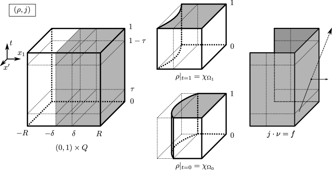
Figure 1. The Eulerian form $(\rho,j)$ of the optimal transport map in $(0,1)\times Q$.

5.2. Preliminaries and key lemmas

In this section we make the above outline more rigorous by introducing fluxes and formulating the aforementioned key lemmas, and then demonstrate that Proposition 4.1 indeed follows from these lemmas.

For a given half-side length $R\in(1,2)$, we consider the subset of trajectories that exit, and the one of those that enter $Q_{R}$:

(5.5) $$\begin{split}{\mathcal{T}}_{+,R}&:=\{X\mid X(1)\not\in Q_{R}\ \mbox{and}\ X(t)\in Q_{R}\ \mbox{for some}\ t\in(0,1)\},\\ {\mathcal{T}}_{-,R}&:=\{X\mid X(0)\not\in Q_{R}\ \mbox{and}\ X(t)\in Q_{R}\ \mbox{for some}\ t\in(0,1)\},\end{split}$$

where here and hereafter $X$ denotes a straight trajectory (in $\mathbb{X}$). Note that these sets are not necessarily disjoint. For $X\in{\mathcal{T}}_{+,R}$ and $X\in{\mathcal{T}}_{-,R}$ we consider the exiting and entering times, respectively,

(5.6) $$\begin{split}t_{+,R}(X)&:=\sup\{t\in(0,1)\mid X(t)\in Q_{R}\}>0,\\ t_{-,R}(X)&:=\inf\{t\in(0,1)\mid X(t)\in Q_{R}\}<1.\end{split}$$

We now define the normal flux $f_{R}$ across $\partial Q_{R}$, as a (signed) measure on $(0,1)\times\partial Q_{R}$ that exists for every (and not just almost every) $R$, by

(5.7) $$\begin{split}&\int_{(0,1)\times\partial Q_{R}}\zeta df_{R}\\ &:=\int_{{\mathcal{T}}_{+,R}}\zeta(t_{+,R},X(t_{+,R}))\mathbb{P}(dX)-\int_{{\mathcal{T}}_{-,R}}\zeta(t_{-,R},X(t_{-,R}))\mathbb{P}(dX),\end{split}$$

where $\zeta\in C([0,1]\times\partial Q_{R})$ is an arbitrary test function and, whenever it is not confusing, we write $t_{\pm,R}=t_{\pm,R}(X)$. In fact, (5.7) holds true for the positive and negative part of the normal flux separately:

(5.8) $$\int_{(0,1)\times\partial Q_{R}}\zeta df_{R,\pm}=\int_{{\mathcal{T}}_{\pm,R}}\zeta(t_{\pm,R},X(t_{\pm,R}))\mathbb{P}(dX).$$

In order to pass from (5.7) to (5.8), we need to show that the two measures on the r.h.s. of (5.8) are orthogonal (mutually singular). Dropping the index $R$, this means that we have to show $(t_{+}(X_{+}),X_{+}(t_{+}(X_{+})))$ $\not=(t_{-}(X_{-}),X_{-}(t_{-}(X_{-})))$ for $\mathbb{P}$-a.e. $X_{+}\in{\mathcal{T}}_{+,R}$ and $X_{-}\in{\mathcal{T}}_{-,R}$. In fact this holds for every $X_{\pm}\in{\mathcal{T}}_{\pm,R}$; we prove it by contradiction so suppose that $(t_{+}(X_{+}),X_{+}(t_{+}(X_{+})))$ $=(t_{-}(X_{-}),X_{-}(t_{-}(X_{-})))$ for some $X_{\pm}$; then, writing $X_{\pm}=tx_{1,\pm}+(1-t)x_{0,\pm}$, we would have $t(x_{1,+}-x_{1,-})$ $=-(1-t)(x_{0,+}-x_{0,-})$ for some $t\in(0,1)$; by monotonicity of ${\rm supp}\pi$ in form of $(x_{1,+}-x_{1,-})\cdot(x_{0,+}-x_{0,-})$ $\geq 0$ this would imply $(x_{0,+},x_{1,+})=(x_{0,-},x_{1,-})$ so $X_{+}=X_{-}$; however, this contradicts the assumption $t_{+}(X_{+})=t_{-}(X_{-})$ since $Q$ is open and hence $t_{+}(X)>t_{-}(X)$ holds for an arbitrary $X\in{\mathcal{T}}_{+,R}\cap{\mathcal{T}}_{-,R}$.

Using the flux $f_{R}$ defined above, we are now able to rigorously formulate the local optimality of $(\rho,j)$ playing a crucial role in our proof.

Lemma 5.1 (Local optimality).

For every $R\in(1,2)$ the measure $f_{R}$ defined by (5.7) coincides with the inner trace of $j$ on $(0,1)\times Q_{R}$ in the sense that for every $\zeta\in C^{1}_{c}([0,1]\times\mathbb{R}^{d})$,

(5.9) $$\int_{(0,1)\times Q_{R}}\partial_{t}\zeta d\rho+\nabla\zeta\cdot dj=\int_{Q_{R}}(\zeta(1,\cdot)\chi_{\Omega_{1}}-\zeta(0,\cdot)\chi_{\Omega_{0}})dx+\int_{(0,1)\times\partial Q_{R}}\zeta df_{R}.$$

In particular, if a pair of measures $(\tilde{\rho},\tilde{j})$ satisfies that for every $\zeta\in C^{1}_{c}([0,1]\times\mathbb{R}^{d})$,

(5.10) $$\int_{(0,1)\times\mathbb{R}^{d}}\partial_{t}\zeta d\tilde{\rho}+\nabla\zeta\cdot d\tilde{j}=\int_{Q_{R}}(\zeta(1,\cdot)\chi_{\Omega_{1}}-\zeta(0,\cdot)\chi_{\Omega_{0}})dx+\int_{(0,1)\times\partial Q_{R}}\zeta df_{R},$$

then the following local optimality holds:

(5.11) $$\int_{(0,1)\times Q_{R}}\frac{1}{\rho}|j|^{2}\leq\int_{(0,1)\times\mathbb{R}^{d}}\frac{1}{\tilde{\rho}}|\tilde{j}|^{2},$$

where the right-hand side is defined through the dual formula (4.18), while the left-hand side is understood pointwise (by using the minimality of $(\rho,j)$).

We proceed with the preparation of our construction. The trajectories we keep are those that cross $(0,1)\times\partial Q$ in $\{x_{1}<\delta\}$ or that exit before $\tau$, or enter after $1-\tau$:

(5.12) $${\mathcal{T}}^{\prime}_{R} :={\mathcal{T}}_{+,R}^{\prime}\cup{\mathcal{T}}_{-,R}^{\prime},$$

$$\mbox{where}\quad\begin{cases}{\mathcal{T}}_{+,R}^{\prime}:=\{X\in{\mathcal{T}}_{+,R}\mid X_{1}(t_{+,R})<\delta\ \mbox{or}\ t_{+,R}<\tau\},\\ {\mathcal{T}}_{-,R}^{\prime}:=\{X\in{\mathcal{T}}_{-,R}\mid X_{1}(t_{-,R})<\delta\ \mbox{or}\ t_{-,R}>1-\tau\}.\end{cases}$$

If we define measures $\rho^{\prime}_{R}$ and $j^{\prime}_{R}$ on $(0,1)\times\mathbb{R}^{d}$ analogously to (4.15) (used later for defining “kept trajectories”, cf. Figure 2), namely for $\zeta\in C(\mathbb{R}^{d})$ and $\xi\in C(\mathbb{R}^{d};\mathbb{R}^{d})$,

(5.13) $$\begin{split}\int\zeta(x)(\rho^{\prime}_{R})_{t}(dx)&:=\int_{{\mathcal{T}}^{\prime}_{R}}\zeta(X(t))\mathbb{P}(dX),\\ \int\xi(x)\cdot(j^{\prime}_{R})_{t}(dx)&:=\int_{{\mathcal{T}}^{\prime}_{R}}\xi(X(t))\cdot\dot{X}(t)\mathbb{P}(dX),\end{split}$$

then (analogously to (5.9)) $(\rho^{\prime}_{R},j^{\prime}_{R})=(dt(\rho^{\prime}_{R})_{t}(dx),dt(j^{\prime}_{R})_{t}(dx))$ distributionally satisfies the continuity equation in $(0,1)\times Q_{R}$ with initial condition $\rho_{0,R}$ at $t=0$, terminal condition $\rho_{1,R}$ at $t=1$, and normal flux $f^{\prime}_{R}$ across $(0,1)\times\partial Q_{R}$ (as in (5.9)), where $\rho_{0,R}$ and $\rho_{1,R}$ are defined in line with (4.14), that is, for $\zeta\in C_{c}(\mathbb{R}^{d})$,

(5.14) $$\begin{split}\int\zeta\rho_{0,R}&:=\int_{{\mathcal{T}}_{+,R}^{\prime}}\zeta(X(0))\mathbb{P}(dX),\\ \int\zeta\rho_{1,R}&:=\int_{{\mathcal{T}}_{-,R}^{\prime}}\zeta(X(1))\mathbb{P}(dX),\end{split}$$

and $f^{\prime}_{R}$ is defined analogously to (5.7), that is, for $\zeta\in C([0,1]\times\partial Q_{R})$,

$$\int_{(0,1)\times\partial Q_{R}}\zeta df_{R}^{\prime}$$

(5.15) $$:=\int_{{\mathcal{T}}_{+,R}^{\prime}}\zeta(t_{+,R},X(t_{+,R}))\mathbb{P}(dX)-\int_{{\mathcal{T}}_{-,R}^{\prime}}\zeta(t_{-,R},X(t_{-,R}))\mathbb{P}(dX).$$

Hence the remaining construction has to connect the initial condition $\chi_{\Omega_{0}}-\rho_{0,R}$ to the terminal condition $\chi_{\Omega_{0}}-\rho_{0,R}$, with the normal flux $f_{R}-f^{\prime}_{R}$. What we have gained by discarding a (small) portion of the trajectories is:

(5.16) $$\begin{split}f_{R}-f^{\prime}_{R}=0\quad\mbox{on}\ \{x_{1}<\delta\},\qquad f_{R}-f^{\prime}_{R}\begin{cases}\leq 0&\mbox{on}\ \{t<\tau\},\\ \geq 0&\mbox{on}\ \{t>1-\tau\}.\end{cases}\end{split}$$

As mentioned above, we split this remaining construction into a construction in $(\tau,1-\tau)\times Q_{R}$, into an “initial construction” in $(0,\tau)\times Q_{R}$, and into a “terminal construction” in $(1-\tau,1)\times Q_{R}$. The initial and terminal constructions require more precise information on $\rho_{0,R}$ and $\rho_{1,R}$. To this purpose, we consider the subsets of those trajectories that exit early or enter late:

(5.17) $$\begin{split}{\mathcal{T}}_{+,R}^{\prime\prime}&:=\{X\in{\mathcal{T}}_{+,R}\mid t_{+,R}<\tau\}\subset{\mathcal{T}}_{+,R}^{\prime},\\ {\mathcal{T}}_{-,R}^{\prime\prime}&:=\{X\in{\mathcal{T}}_{-,R}\mid t_{-,R}>1-\tau\}\subset{\mathcal{T}}_{-,R}^{\prime},\end{split}$$

and the corresponding densities: for $\zeta\in C_{c}(\mathbb{R}^{d})$,

(5.18) $$\begin{split}\int\zeta\rho_{0,R}^{\prime}&:=\int_{{\mathcal{T}}_{+,R}^{\prime\prime}}\zeta(X(0))\mathbb{P}(dX),\\ \int\zeta\rho_{1,R}^{\prime}&:=\int_{{\mathcal{T}}_{-,R}^{\prime\prime}}\zeta(X(1))\mathbb{P}(dX).\end{split}$$

We finally note that the measures $f_{R}$ and $f_{R}^{\prime}$ have Hausdorff densities on $(0,1)\times\partial Q_{R}$ for a.e. $R\in(1,2)$. It follows from Lemma 5.1 that for every $R\in(1,2)$, the inner normal trace of $j$ (as a measure) exists and coincides with $f_{R}$. Since in addition $j$ has a (square integrable) Lebesgue density, which we denote again by $j$, the Hausdorff density of this inner trace coincides with $\nu\cdot j$ for a.e. $R\in(1,2)$; in fact, this is true for every Lebesgue point $R$ of $j$, seen as an element of $L^{2}((1,2);L^{2}((0,1)\times\partial Q_{R}))$. As a consequence, for a.e. $R\in(1,2)$, $\nu\cdot j$ is the Hausdorff density of $f_{R}$. In addition, the square integrability (of the density) of $f_{R}$ obviously transmits to $f_{R}^{\pm}$. We then learn from (5.8) that this transmits to the two r.h.s. expressions. Since these clearly dominate the respective r.h.s. expressions in (5.14), also $f_{R}^{\prime}$ is square integrable.

We are now in a position to choose a good half-side length $R$ (slice) such that the quantities introduced above are well estimated, that is, behave like on average (with respect to $R$). The proof is given in Section 5.3.

Lemma 5.2 (Good slices).

For any fixed $\tau\in(0,1)$, there exists $R\in(1,2)$ such that

(5.19) $$\int_{(0,1)\times\partial Q_{R}}f_{R}^{2} \lesssim E,$$

(5.20) $$\int_{(0,1)\times\mathbb{R}^{d}}\frac{1}{\rho^{\prime}_{R}}|j^{\prime}_{R}|^{2} \lesssim ME,$$

(5.21) $$\rho_{0,R},\rho_{1,R}\leq 1,\quad\int_{\mathbb{R}^{d}}{\rm dist}(\cdot,\partial Q_{R})(\rho_{0,R}+\rho_{1,R}) \lesssim E,$$

(5.22) $$\rho_{0,R}^{\prime},\rho_{1,R}^{\prime}\leq 1,\quad\int_{\mathbb{R}^{d}}{\rm dist}(\cdot,\partial Q_{R})(\rho_{0,R}^{\prime}+\rho_{1,R}^{\prime}) \lesssim\tau^{2}E.$$

We remark that in order to get the coefficient $\tau^{2}$ in (5.22) we will use the fact that the initial points (resp. the target points) of the trajectories exiting early (resp. entering late) are “close” to the boundary $\partial Q_{R}$. This might not be true for the trajectories exiting late and entering early; this is why we deal with those trajectories separately.

From now on, we drop the index $R$. In fact, for (notational) simplicity, we treat $R$ as being unity $R=1$.

We now turn to our main estimates. The Poisson equation we use for approximating the velocity $j/\rho$ is:

(5.23) $$\begin{cases}\Delta\phi=c&\mbox{in}\ Q\cap\{x_{1}>0\},\\ \nu\cdot\nabla\phi=\bar{f}&\mbox{on}\ \partial Q\cap\{x_{1}>0\},\\ \nu\cdot\nabla\phi=0&\mbox{on}\ Q\cap\{x_{1}=0\},\end{cases}$$

where we have introduced the following abbreviation of the boundary flux, cf. (5.7) and (5.2):

(5.24) $$\bar{f}:=\int_{0}^{1}(f-f^{\prime})dt\quad\mbox{on}\ \partial Q,$$

and $c$ is the constant that makes the problem solvable; throughout this section, $\nu$ denotes the outer normal of a domain under consideration. Because $\partial_{1}\phi$ vanishes for $x_{1}=0$, we may extend $\nabla\phi$ harmonically onto $Q$ by reflection, cf. (4.22).

The next lemma shows that in a certain sense, $j-\rho\nabla\phi$ and $\nabla\phi$ are almost orthogonal, cf. (5.25). The proof is given in Section 5.4.

Lemma 5.3 (Approximate orthogonality).

Given $\tau\in(0,1/4)$, we have

(5.25) $$\begin{split}\int_{(0,1)\times Q}\frac{1}{\rho}|j-\rho\nabla\phi|^{2}&-\left(\int_{(0,1)\times Q}\frac{1}{\rho}|j|^{2}-\int_{Q\cap\{x_{1}>-\delta\}}|\nabla\phi|^{2}\right)\\ &\lesssim E^{\frac{1}{2}}\delta+(\tau+\delta)^{\frac{1}{2}}E,\end{split}$$

and also

(5.26) $$\int_{Q}|\nabla\phi|^{2}\lesssim E.$$

We then turn to the construction of a competitor, which is based on the solution to the following modified equation:

(5.27) $$\begin{cases}\Delta\tilde{\phi}=\tilde{c}&\mbox{in}\ Q\cap\{x_{1}>\delta\},\\ \nu\cdot\nabla\tilde{\phi}=\bar{f}&\mbox{on}\ \partial Q\cap\{x_{1}>\delta\},\\ \nu\cdot\nabla\tilde{\phi}=\bar{g}&\mbox{on}\ Q\cap\{x_{1}=\delta\},\end{cases}$$

where next to (5.24) we have also introduced the abbreviation, cf. (4.3):

(5.28) $$\bar{g}:=g_{0}-g_{1}\quad\mbox{on}\;Q\cap\{x_{1}=\delta\}\cong Q^{\prime}:=(-1,1)^{d-1},$$

and $\tilde{c}$ is the constant that makes the problem solvable.

The final lemma states that there exists a competitor of transport cost close to the Dirichlet integral of $\nabla\tilde{\phi}$, cf. (5.4), where it matters that the r.h.s. of (5.4) is super-linear in $E+\delta^{2}$ (after optimization in $\tau$), and also states that $\nabla\phi$ and $\nabla\tilde{\phi}$ have comparable Dirichlet energies, cf. (5.30). The proof is given in Section 5.5.

Lemma 5.4 (Construction).

Given $\tau\in(0,1/4)$, there exists an admissible pair $(\tilde{\rho},\tilde{j})$ (i.e., satisfying (5.10)) concentrated on $(0,1)\times\overline{Q}$ such that

$$\int_{(0,1)\times\mathbb{R}^{d}}\frac{1}{\tilde{\rho}}|\tilde{j}|^{2}-\int_{Q\cap\{x_{1}>\delta\}}|\nabla\tilde{\phi}|^{2}$$

(5.29) $$\lesssim\tau(E+\delta^{2})+(E+\delta^{2})^{\frac{d+2}{d+1}}+\delta^{3}+\frac{(M+\delta)^{\frac{1}{d-1}}}{\tau}E.$$

In case of $d=2$, the exponent $\frac{1}{d-1}$, which would be equal to $1$, has to be replaced by an (in fact, any) exponent $\beta<1$. In addition,

(5.30) $$\int_{Q\cap\{x_{1}>\delta\}}|\nabla\tilde{\phi}|^{2}-\int_{Q\cap\{x_{1}>-\delta\}}|\nabla\phi|^{2}\lesssim E^{\frac{1}{2}}\delta+\delta^{2}.$$

We conclude this subsection by demonstrating that the above lemmas indeed imply Proposition 4.1.

Proof of Proposition 4.1.

Within this proof we restore the index $R\in(1,2)$ taken in Lemma 5.2 for clarity.

We take $\phi\in C^{\infty}(Q_{R})$ as defined in (5.23) and by reflection, and prove that this $\phi$ (restricted to $\overline{Q_{1}}$) is the desired harmonic gradient. Since $\nabla\phi$ is harmonic and satisfies (4.22) by definition, and (4.21) follows from (5.26), it only remains to establish (4.20). We start from (5.25) and (5.30) in Lemma 5.3 which combine to

$$\int_{(0,1)\times Q_{R}}\frac{1}{\rho}|j-\rho\nabla\phi|^{2}-\left(\int_{(0,1)\times Q_{R}}\frac{1}{\rho}|j|^{2}-\int_{Q_{R}\cap\{x_{1}>\delta\}}|\nabla\tilde{\phi}|^{2}\right)$$

$$\lesssim E^{\frac{1}{2}}\delta+\delta^{2}+(\tau+\delta)^{\frac{1}{2}}E.$$

We then turn to Lemma 5.4 and appeal to the local optimality in Lemma 5.1, namely

$$\int_{(0,1)\times Q_{R}}\frac{1}{\rho}|j|^{2}\leq\int_{(0,1)\times\mathbb{R}^{d}}\frac{1}{\tilde{\rho}}|\tilde{j}|^{2},$$

and to (5.4) to obtain

$$\int_{(0,1)\times Q_{R}}\frac{1}{\rho}|j-\rho\nabla\phi|^{2}\lesssim E^{\frac{1}{2}}\delta+\delta^{2}$$

(5.31) $$+(\tau+\delta)^{\frac{1}{2}}(E+\delta^{2})+(E+\delta^{2})^{\frac{d+2}{d+1}}+\frac{(M+\delta)^{\frac{1}{d-1}}}{\tau}E.$$

Given $\varepsilon\in(0,1]$, for the very first r.h.s. term $E^{\frac{1}{2}}\delta$ we apply Young’s inequality to control it by $\varepsilon E+\frac{1}{\varepsilon}\delta^{2}\lesssim\varepsilon E+\frac{1}{\varepsilon}D$ as desired, cf. (5.2). The remaining r.h.s. terms can all be made $\lesssim\varepsilon E+\delta^{2}$ so that $\lesssim\varepsilon E+D$; namely we choose $\tau$ so small that $(\tau+\delta)^{\frac{1}{2}}\leq\varepsilon$, cf. (5.1), and since $E+D\ll_{\varepsilon}1$ so that both

$$(E+\delta^{2})^{\frac{1}{d+1}}\stackrel{{\scriptstyle\eqref{ao53}}}{{\lesssim}}(E+D)^{\frac{1}{d+1}}\leq\varepsilon,\quad\frac{(M+\delta)^{\frac{1}{d-1}}}{\tau}\stackrel{{\scriptstyle\eqref{ao87},\eqref{ao53}}}{{\lesssim}}\frac{(E^{\frac{1}{d+2}}+D^{\frac{1}{2}})^{\frac{1}{d-1}}}{\tau}\leq\varepsilon.$$

The arbitrariness of $\varepsilon$ implies the assertion. ∎

In the remainder of this section we prove all the above lemmas.

5.3. Local optimality and good slices lemma

In this subsection we prove Lemmas 5.1 and 5.2 in line with [15].

Proof of Lemma 5.1.

By an approximation argument we may use the (discontinuous) test functions $\chi_{Q_{R}}\partial_{t}\zeta$ and $\chi_{Q_{R}}\nabla\zeta$ in the definition of $(\rho,j)$, cf. (4.15), for an arbitrary $\zeta\in C^{1}_{c}([0,1]\times\mathbb{R}^{d})$. Hence we have

$$\int_{(0,1)\times Q_{R}}\partial_{t}\zeta d\rho+\nabla\zeta\cdot dj$$

$$=\int_{0}^{1}\int_{\{X(t)\in Q_{R}\}}\left(\partial_{t}\zeta(t,X(t))+\nabla\zeta(t,X(t))\cdot\dot{X}(t)\right)\mathbb{P}(dX)dt$$

$$=\int_{\mathcal{T}_{R}}\left(\zeta(t_{+},X(t_{+}))-\zeta(t_{-},X(t_{-}))\right)\mathbb{P}(dX),$$

where $\mathcal{T}_{R}:=\{X\mid X(t)\in Q_{R}\ \mbox{for some }t\}$, and the exiting and entering times $t_{\pm,R}=t_{\pm,R}(X)$ are understood as in (5.6) even if $X$ is totally contained in $Q_{R}$. Since $\mathcal{T}_{R}$ is decomposed into the disjoint sets $\{X(1)\in Q_{R}\}$ and $\mathcal{T}_{+,R}=\mathcal{T}_{R}\cap\{X(1)\not\in Q_{R}\}$, cf. (5.5), we deduce from the marginal condition (4.14) and (5.8) that

$$\int_{\mathcal{T}_{R}}\zeta(t_{+,R},X(t_{+,R}))\mathbb{P}(dX)=\int_{Q_{R}}\zeta(1,\cdot)\chi_{\Omega_{1}}dx+\int_{(0,1)\times\partial Q_{R}}\zeta df_{R,+}.$$

Similarly we have

$$\int_{\mathcal{T}_{R}}\zeta(t_{-,R},X(t_{-,R}))\mathbb{P}(dX)=\int_{Q_{R}}\zeta(0,\cdot)\chi_{\Omega_{0}}dx+\int_{(0,1)\times\partial Q_{R}}\zeta df_{R,-},$$

and hence by the definition of $f_{R}$, cf. (5.7), we obtain (5.9).

We finally prove local optimality (5.11). Since by (5.9) and (5.10) the pair $(\hat{\rho},\hat{j}):=(\tilde{\rho},\tilde{j})+(\rho,j)|_{(0,1)\times(\mathbb{R}^{d}\setminus\overline{Q_{R}})}$ is a competitor in (4.17), and since by definition (4.18) the transportation cost is sub-additive, we have

$$\int_{(0,1)\times\mathbb{R}^{d}}\frac{1}{\rho}|j|^{2}\leq\int_{(0,1)\times\mathbb{R}^{d}}\frac{1}{\hat{\rho}}|\hat{j}|^{2}\leq\int_{(0,1)\times\mathbb{R}^{d}}\frac{1}{\tilde{\rho}}|\tilde{j}|^{2}+\int_{(0,1)\times(\mathbb{R}^{d}\setminus\overline{Q_{R}})}\frac{1}{\rho}|j|^{2}.$$

The additivity of the classical integral $\int\frac{1}{\rho}|j|^{2}$ completes the proof. ∎

Proof of Lemma 5.2.

We start with (5.19) by arguing that

$$\int_{1}^{2}\int_{(0,1)\times\partial Q_{R}}f_{R}^{2}dR\leq E.$$

Indeed, since we have $f_{R}=\nu\cdot j$ a.e. on $\partial Q_{R}$ for a.e. $R\in(1,2)$, cf. (5.9), we obtain from the co-area formula $\int_{Q_{2}\setminus Q_{1}}=\int_{1}^{2}\int_{\partial Q_{R}}dR$ that

$$\int_{1}^{2}\int_{(0,1)\times\partial Q_{R}}f_{R}^{2}dR\leq\int_{(0,1)\times Q_{2}}(\nu\cdot j)^{2}\stackrel{{\scriptstyle\eqref{ao54}}}{{\leq}}\int_{(0,1)\times Q_{2}}\frac{1}{\rho}|j|^{2}\leq E,$$

where the last estimate follows since the $L^{\infty}$-bounds (4.7) and (4.11) yield that there are no trajectories going through $Q_{2}$ such that $x_{0}\not\in Q_{8}$ and $x_{1}\not\in Q_{8}$.

Turning to (5.20) we show

$$\int_{1}^{2}\int_{(0,1)\times\mathbb{R}^{d}}\frac{1}{\rho_{R}^{\prime}}|j_{R}^{\prime}|^{2}dR\leq ME.$$

Indeed, it follows from the definition of $(\rho_{R}^{\prime},j_{R}^{\prime})$, cf. (5.13), that

$$\int_{(0,1)\times\mathbb{R}^{d}}\frac{1}{\rho_{R}^{\prime}}|j_{R}^{\prime}|^{2}\leq\int_{{\mathcal{T}}_{R}^{\prime}}|X(1)-X(0)|^{2}\mathbb{P}(dX)$$

$$\stackrel{{\scriptstyle\eqref{ao66}}}{{\leq}}\int_{{\mathcal{T}}_{+,R}\cup{\mathcal{T}}_{-,R}}|X(1)-X(0)|^{2}\mathbb{P}(dX)\stackrel{{\scriptstyle\eqref{ao67}}}{{=}}\int I_{X,R}|X(1)-X(0)|^{2}\mathbb{P}(dX),$$

where $I_{X,R}$ denotes the characteristic function of the set

$$\left\{X\left|\ |X(1)|_{\infty}\geq R>\min_{t}|X(t)|_{\infty}\;{\rm or}\;|X(0)|_{\infty}\geq R>\min_{t}|X(t)|_{\infty}\right\}\right.,$$

and $|\cdot|_{\infty}$ denotes the norm in which the cube is the ball. We now integrate in $R$: Using that ($I_{X,R}=1$ $\Longrightarrow$ $\max_{t}|X(t)|_{\infty}$ $\geq R$ $>\min_{t}|X(t)|_{\infty}$), appealing to $\max_{t}|X(t)|_{\infty}-\min_{t}|X(t)|_{\infty}\leq\max_{t^{\prime},t}|X(t^{\prime})-X(t)|$, inferring from (4.7) that

(5.32) $$\max_{t^{\prime},t\in(0,1)}|X(t^{\prime})-X(t)|\leq M\quad\mbox{provided}\;X(0)\in Q_{4}\;\mbox{or}\;X(1)\in Q_{4},$$

and noting that by (4.11) the set of (straight) trajectories $X$ with $X(t)\in Q_{2}$ for some $t$ is contained in the set of trajectories with $X(1)\in Q_{4}$ or $X(0)\in Q_{4}$, we have

$$\int_{1}^{2}\int_{(0,1)\times\mathbb{R}^{d}}\frac{1}{\rho_{R}^{\prime}}|j_{R}^{\prime}|^{2}dR$$

$$\leq M\int_{\{X(1)\in Q_{4}\}\cup\{X(0)\in Q_{4}\}}|X(1)-X(0)|^{2}\mathbb{P}(dX)\lesssim ME,$$

where for the last estimate we directly inferred from (4.1) that

(5.33) $$\int_{\{X(0)\in Q_{4}\}\cup\{X(1)\in Q_{4}\}}|X(1)-X(0)|^{2}\mathbb{P}(dX)\lesssim E.$$

We now turn to the proof of (5.21), and (5.22). Appealing to symmetry, we restrict ourselves to $\rho_{0}$ and $\rho_{0}^{\prime}$. The pointwise bounds in form of $0\leq\rho_{0}^{\prime}\leq\rho_{0}\leq 1$ follow via definitions (5.14) and (5.18) from (4.14). For the integral bound we will restrict ourselves to (5.22), since (5.21) follows from the latter for $\tau=\frac{1}{2}$, and show that

$$\int_{1}^{2}\int_{\mathbb{R}^{d}}{\rm dist}(\cdot,\partial Q_{R})\rho_{0,R}^{\prime}dR\leq\tau^{2}E.$$

By definition (5.18), we have

$$\int_{\mathbb{R}^{d}}{\rm dist}(\cdot,\partial Q_{R})\rho_{0,R}^{\prime}=\int_{{\mathcal{T}}_{+,R}^{\prime\prime}}|R-|X(0)|_{\infty}|\mathbb{P}(dX).$$

By definition (5.17) of ${\mathcal{T}}_{+,R}^{\prime\prime}$ and (5.6) of $t_{+,R}$ we have for $X\in{\mathcal{T}}_{+,R}^{\prime\prime}$ that $\sup_{t<\tau}|X|_{\infty}$ $\geq R$ $>\inf_{t<\tau}|X|_{\infty}$ and thus in particular

$$|R-|X(0)|_{\infty}|\leq\sup_{t<\tau}|X|_{\infty}-\inf_{t<\tau}|X|_{\infty}\leq\tau|X(1)-X(0)|,$$

where the last estimate follows since trajectories are straight. Hence we obtain from integrating in $R$ (and noting the implicitly-multiplied characteristic function on the set $\{(X,R)\mid\sup_{t<\tau}|X|_{\infty}\geq R>\inf_{t<\tau}|X|_{\infty}\}$ as above),

$$\int_{1}^{2}\int_{\mathbb{R}^{d}}{\rm dist}(\cdot,\partial Q_{R})\rho_{0,R}^{\prime}dR\leq\tau^{2}\int_{\{X\mid\exists t,\ X(t)\in Q_{2}\}}|X(1)-X(0)|^{2}\mathbb{P}(dX).$$

By (4.11) again, the r.h.s. integral is estimated by $E$, cf. (5.33). ∎

5.4. Approximate orthogonality

Proof of Lemma 5.3.

By the definition of the integrand $\frac{1}{\rho}|j|^{2}$, the support condition (5.3) implies that also $\frac{1}{\rho}|j-\rho\nabla\phi|^{2}$ and $\frac{1}{\rho}|j|^{2}$ are supported in $\{x_{1}>-\delta\}$. Hence we obtain from expanding the square:

$$\int_{(0,1)\times Q}\frac{1}{\rho}|j-\rho\nabla\phi|^{2} =\int_{(0,1)\times Q}\frac{1}{\rho}|j|^{2}-\int_{(0,1)\times(Q\cap\{x_{1}>-\delta\})}(2-\rho)|\nabla\phi|^{2}$$

(5.34) $$+2\int_{(0,1)\times(Q\cap\{x_{1}>-\delta\})}(\nabla\phi-j)\cdot\nabla\phi.$$

Therefore by $\rho\leq 1$, cf. (4.19), for (5.25) it remains to bound the last term.

In what follows we first prepare some trace estimates for later use, then rephrase the above last term so that the estimates in the previous step are applicable, and finally complete the proof by estimating the rephrased one; estimate (5.26) is shown in the middle of Step 1.

Step 1: Trace estimates and control of boundary fluxes. We first note

(5.35) $$\int_{(0,1)\times\partial Q}(f-f^{\prime})^{2}+\int_{\partial Q}\bar{f}^{2}\lesssim E.$$

Indeed, since we have a splitting $f^{\prime}=f^{\prime}_{+}-f^{\prime}_{-}$ with $0\leq f_{\pm}^{\prime}\leq f_{\pm}$, cf. (5.8) and (5.2), and $f_{\pm}$ being the positive and negative parts of $f$ as was shown right after (5.8), we have

(5.36) $$|f-f^{\prime}|\leq|f|,\quad|f^{\prime}|\leq|f|,$$

so that (5.35) follows from definition (5.24) and estimate (5.19).

By standard $L^{2}$-based maximal regularity theory for (5.23) in terms of the Neumann data (see Remark 5.5 below for details), we have

(5.37) $$\sup_{x_{1}}\int_{Q^{\prime}}|\nabla\phi(x_{1},\cdot)|^{2}\lesssim\int_{\partial Q}\bar{f}^{2}\stackrel{{\scriptstyle\eqref{ao48}}}{{\lesssim}}E,$$

where $Q^{\prime}=\{x^{\prime}\in(-1,1)^{d-1}\}$ denotes the $(d-1)$-dimensional cube in tangential direction; we call (5.37) a maximal regularity estimate since the left and right hand side have the same scaling. Estimate (5.26) now follows directly from (5.37).

We further post-process (5.37): For a test function $\zeta$ on $Q\cap\{x_{1}>a\}$ (for some $a\in(-1/2,1/2)$), combining the Poincaré-trace estimate in $(d-1)$ dimensions

$$\int_{\partial Q^{\prime}}\zeta^{2}+\int_{Q^{\prime}}\zeta^{2}\lesssim\int_{Q^{\prime}}|\nabla^{\prime}\zeta|^{2}+\big{|}\int_{Q^{\prime}}\zeta\big{|}^{2},$$

with the obvious

$$\sup_{x_{1}}\big{|}\int_{Q^{\prime}}\zeta\big{|}^{2}\lesssim\sup_{x_{1}}\int_{Q^{\prime}}|\partial_{1}\zeta|^{2}+\big{|}\int_{Q\cap\{x_{1}>a\}}\zeta\big{|}^{2},$$

we obtain

(5.38) $$\sup_{x_{1}}\big{(}\int_{\partial Q^{\prime}}\zeta^{2}+\int_{Q^{\prime}}\zeta^{2}\big{)}\lesssim\sup_{x_{1}}\int_{Q^{\prime}}|\nabla\zeta|^{2}+\big{|}\int_{Q\cap\{x_{1}>a\}}\zeta\big{|}^{2}.$$

Applying this to $\zeta=\phi$ on $Q\cap\{x_{1}>-\delta\}$, where we normalize such that

(5.39) $$\int_{Q\cap\{x_{1}>-\delta\}}\phi=0,$$

we obtain by (5.37) the (co-dimension two) estimate

(5.40) $$\sup_{x_{1}}\left(\int_{\partial Q^{\prime}}\phi^{2}+\int_{Q^{\prime}}\phi^{2}\right)\lesssim E.$$

Step 2: Rephrasing in terms of $\phi$ and boundary fluxes. We now rephrase the last term in (5.4) in terms of $\phi$ and normal fluxes on the boundary. Integrating in $t$ the continuity equation and recalling the normal flux boundary data $f$ for $j$, and the initial data $\chi_{\Omega_{0}}$ and terminal data $\chi_{\Omega_{1}}$ for $\rho$ (namely taking constant-in-$t$ test functions $\zeta$ in (5.9)), we see that $\bar{j}:=\int_{0}^{1}jdt$ distributionally satisfies

(5.41) $$\begin{cases}\nabla\cdot\bar{j}=-g&\mbox{in}\ Q\cap\{x_{1}>-\delta\},\\ \nu\cdot\bar{j}=\int_{0}^{1}fdt&\mbox{on}\ \partial Q\cap\{x_{1}>-\delta\},\\ \nu\cdot\bar{j}=0&\mbox{on}\ Q\cap\{x_{1}=-\delta\},\end{cases}$$

where we have introduced the characteristic function $g:=\chi_{\Omega_{1}}-\chi_{\Omega_{0}}$, that is,

(5.42) $$g(x):=\begin{cases}1&\mbox{for}\ g_{1}(x^{\prime})<x_{1}<g_{0}(x^{\prime}),\\ -1&\mbox{for}\ g_{0}(x^{\prime})<x_{1}<g_{1}(x^{\prime}),\\ 0&\mbox{else},\end{cases}$$

in the first line, cf. (4.3), and used (5.3) for the last item. Therefore, appealing to (5.23) (in its reflected form), to (5.39), and to (5.41) tested by $\phi$, we obtain for the last term in (5.4)

$$\int_{(0,1)\times(Q\cap\{x_{1}>-\delta\})}(\nabla\phi-j)\cdot\nabla\phi=\int_{Q\cap\{x_{1}>-\delta\}}(\nabla\phi-\bar{j})\cdot\nabla\phi$$

$$\stackrel{{\scriptstyle\eqref{ao09},\eqref{ao115}}}{{=}}-\int_{Q\cap\{x_{1}>-\delta\}}g\phi+\int_{\partial Q\cap\{x_{1}>-\delta\}}\phi\left(\bar{f}-\int_{0}^{1}fdt\right)-\int_{Q\cap\{x_{1}=-\delta\}}\phi\partial_{1}\phi.$$

We claim that we may rewrite the last term as

$$-\int_{Q\cap\{x_{1}=-\delta\}}\phi\partial_{1}\phi$$

(5.43) $$=\int_{-\delta}^{0}\int_{Q^{\prime}}\nabla^{\prime}\phi(-\delta,x^{\prime})\cdot\nabla^{\prime}\phi(x_{1},x^{\prime})dx^{\prime}dx_{1}+\delta c\int_{Q^{\prime}}\phi(-\delta,x^{\prime})dx^{\prime}.$$

Indeed, we obtain (5.4) by using the homogeneous flux boundary condition in (5.23) in form of

$$-\partial_{1}\phi(-\delta,x^{\prime})=\int_{-\delta}^{0}\partial_{1}^{2}\phi(x_{1},x^{\prime})dx_{1},$$

combining it with the Poisson equation in form of

$$\int_{-\delta}^{0}\partial_{1}^{2}\phi(x_{1},x^{\prime})dx_{1}=\delta c-\int_{-\delta}^{0}\Delta^{\prime}\phi(x_{1},x^{\prime})dx_{1},$$

and appealing to integration by parts in $x^{\prime}$ in form of

$$-\int_{Q^{\prime}}\phi(-\delta,x^{\prime})\int_{-\delta}^{0}\Delta^{\prime}\phi(x_{1},x^{\prime})dx_{1}dx^{\prime}=\int_{-\delta}^{0}\int_{Q^{\prime}}\nabla^{\prime}\phi(-\delta,x^{\prime})\cdot\nabla^{\prime}\phi(x_{1},x^{\prime})dx^{\prime}dx_{1},$$

where there are no boundary terms here since $\bar{f}$ vanishes for $x_{1}<\delta$ by (5.16) and (5.24). Hence we rearrange the terms as follows

$$\int_{(0,1)\times(Q\cap\{x_{1}>-\delta\})}(\nabla\phi-j)\cdot\nabla\phi$$

$$=-\int_{Q\cap\{|x_{1}|<\delta\}}g\phi-\int_{\partial Q\cap\{|x_{1}|<\delta\}}\phi\int_{0}^{1}fdt+\int_{\partial Q\cap\{x_{1}>\delta\}}\phi\left(\bar{f}-\int_{0}^{1}fdt\right)$$

$$\quad+\int_{Q\cap\{-\delta<x_{1}<0\}}(\nabla^{\prime}\phi|_{x_{1}=-\delta})\cdot\nabla^{\prime}\phi+\delta c\int_{Q\cap\{x_{1}=-\delta\}}\phi$$

$$=:T_{1}+T_{2}+T_{3}+T_{4}+T_{5},$$

where we also used ${\rm supp}g\subset\{|x_{1}|\leq\delta\}$, cf. (5.42) and (5.1).

Step 3: Main estimates. We finally estimate the above $T_{1},\dots,T_{5}$. Using $|g|\leq 1$ and (5.40), we see that $T_{1}$ is responsible for the leading-order term in (5.25):

$$|T_{1}|\lesssim E^{\frac{1}{2}}\delta.$$

For $T_{2}$ we note that by the Cauchy-Schwarz inequality

$$|T_{2}|\leq\left(\Big{(}\sup_{x_{1}}\int_{\partial Q^{\prime}}\phi^{2}\Big{)}2\delta\int_{(0,1)\times\partial Q}f^{2}\right)^{1\over 2}\stackrel{{\scriptstyle\eqref{ao07},\eqref{ao43}}}{{\lesssim}}\delta^{\frac{1}{2}}E,$$

which is contained in the r.h.s. of (5.25). We turn to $T_{3}$ and note that by definition (5.24) of $\bar{f}$ we have $\int_{0}^{1}fdt-\bar{f}=\int_{0}^{1}f^{\prime}dt$; by definition (5.2) of $f^{\prime}$ we have, provided $x_{1}>\delta$, that $f^{\prime}$ vanishes unless $t\in(0,\tau)\cup(1-\tau,1)$, so that

$$\int_{\partial Q\cap\{x_{1}>\delta\}}\left(\int_{0}^{1}f^{\prime}dt\right)^{2}\leq 2\tau\int_{(0,1)\times\partial Q}f^{\prime 2}.$$

Finally by (5.36) we may apply (5.19), to the effect of $\int_{(0,1)\times\partial Q}f^{\prime 2}\lesssim E$. In conclusion we have

$$\int_{\partial Q\cap\{x_{1}>\delta\}}\left(\bar{f}-\int_{0}^{1}fdt\right)^{2}\lesssim\tau E,$$

so that we obtain with help of the Cauchy-Schwarz inequality and (5.40)

$$|T_{3}|\lesssim\tau^{\frac{1}{2}}E,$$

in line with (5.25). We directly obtain from the Cauchy-Schwarz inequality and (5.37):

$$|T_{4}|\lesssim\delta E,$$

in agreement with (5.25) (since $\delta\ll 1$). Finally, for $T_{5}$ we note that from (5.23) we have $c|Q\cap\{x_{1}>0\}|$ $=\int_{\partial Q\cap\{x_{1}>0\}}\bar{f}$, so that by (5.35) we get

(5.44) $$|c|\lesssim E^{\frac{1}{2}},$$

hence in conjunction with (5.40) we likewise obtain

$$|T_{5}|\lesssim\delta E,$$

completing the proof. ∎

Remark 5.5 ($L^{2}$-maximal regularity).

For the reader’s convenience, we sketch the argument for (5.37). By the triangle inequality, it is enough to consider Neumann data that are supported on one of the $2d$ faces of the box $Q$, which we take without loss of generality to be the cube $(0,2)^{d}$ and $\{x_{1}=2\}$ to be that face. By even reflection, which preserves the equation, we may replace the cube by a slab $S:=(-2,2)\times[-2,2)^{d-1}$ of thickness 4 and (lateral) periodicity with period 4. By treating constant Neumann data explicitly, we may restrict to the case of Neumann data of vanishing spatial average. By the boundedness of the Neumann-to-Dirichlet map (which easily may be seen for instance on the Fourier side) we may assume that we have a harmonic function $\phi$ on the periodic slab $S$ of which we control $\int_{\partial S}|\nabla\phi|^{2}$ on the boundary $\partial S:=\{-2,2\}\times[-2,2)^{d-1}$ and where we seek control on faces $\int_{S\cap\{x_{i}=\mathrm{const.}\}}|\nabla\phi|^{2}$. Hence we may replace (any component of) the gradient $\nabla\phi$ by a harmonic function $\phi$ in both $L^{2}$-norms. Control of tangential faces $\int_{S\cap\{x_{1}=\mathrm{const.}\}}\phi^{2}$ can easily be seen, for instance on the Fourier side. For a perpendicular face, say $\int_{S\cap\{x_{2}=0\}}\phi^{2}$, the argument goes as follows: By the triangle inequality, we may assume that $\phi$ vanishes on the lower boundary $\{x_{1}=-2\}$. Let $\psi$ be such that $\partial_{1}\psi=\phi$ and that it vanishes on the upper boundary $\{x_{1}=2\}$. We easily see, for instance by considering the Fourier transform in the tangential directions $x^{\prime}$ to obtain a representation of $\phi$ in terms of its boundary data, that the control of the boundary data in terms of $\int_{\partial S\cap\{x_{1}=2\}}\phi^{2}$ yields control of the harmonic extension $\phi$ (and its anti-derivative $\psi$) in the weighted $L^{2}_{x^{\prime}}$-based norm

$$\int_{S}\Big{(}\frac{1}{2-x_{1}}(\partial_{2}\psi)^{2}+(2-x_{1})(\partial_{1}\phi)^{2}+\phi^{2}\Big{)},$$

where the power of the distance to the boundary $\{x_{1}=2\}$ is optimal (for the first two terms) and dictated by scaling. By Young’s inequality, this yields control of $\int_{(-2,2)^{d}}(|\partial_{2}\psi\partial_{1}\phi|+\phi^{2}).$ By an integration by parts in $x_{1}$ using $\phi|_{\{x_{1}=-2\}}=0$ and $\psi|_{\{x_{1}=2\}}=0$, this yields control of

$$\int_{-2}^{2}\Big{(}\big{|}\int_{(-2,2)^{d-1}}\phi\partial_{2}\phi dx^{\prime\prime}\big{|}+\int_{(-2,2)^{d-1}}\phi^{2}dx^{\prime\prime}\Big{)}dx_{2},$$

where we have set $x^{\prime\prime}:=(x_{1},x_{3},\cdots,x_{d})$. Because of

$$\frac{d}{dx_{2}}\int_{(-2,2)^{d-1}}\phi^{2}dx^{\prime\prime}=2\int_{(-2,2)^{d-1}}\phi\partial_{2}\phi dx^{\prime\prime},$$

this yields the desired control of $\sup_{x_{2}}\int_{(-2,2)^{d-1}}\phi^{2}dx^{\prime\prime}$.

5.5. Construction of a competitor

Proof of Lemma 5.4.

We first independently address estimate (5.30), and then turn to the construction of an admissible competitor $(\tilde{\rho},\tilde{j})$. As is described in Section 5.1, we will construct $(\tilde{\rho},\tilde{j})$ of the form (5.4), where all the r.h.s. terms are concentrated on $(0,1)\times Q$ except for the singular construction $(\rho^{\mathrm{sing}},j^{\mathrm{sing}})$ concentrated on $(0,1)\times\partial Q$, and then appeal to sub-additivity of the cost functional. The construction is divided into a number of steps.

Step 1: Comparability of the energies of $\phi$ and $\tilde{\phi}$. For (5.30), obviously, it is sufficient to estimate

(5.45) $$T:=\int_{Q\cap\{x_{1}>\delta\}}|\nabla\tilde{\phi}|^{2}-\int_{Q\cap\{x_{1}>\delta\}}|\nabla\phi|^{2}=\int_{Q\cap\{x_{1}>\delta\}}\nabla(\tilde{\phi}+\phi)\cdot\nabla(\tilde{\phi}-\phi).$$

By an integration by parts and (5.23) and (5.27), $T$ can be rewritten as

$$T=-\int_{Q\cap\{x_{1}>\delta\}}(\tilde{\phi}+\phi)(\tilde{c}-c)+\int_{Q\cap\{x_{1}=\delta\}}(\tilde{\phi}+\phi)(\bar{g}+\partial_{1}\phi).$$

As for (5.4), we rewrite the term $\int_{Q\cap\{x_{1}=\delta\}}(\tilde{\phi}+\phi)\partial_{1}\phi$, leading to

$$T =-(\tilde{c}-c)\int_{Q\cap\{x_{1}>\delta\}}(\tilde{\phi}+\phi)+\int_{Q\cap\{x_{1}=\delta\}}(\tilde{\phi}+\phi)(\bar{g}+2\delta c)$$

$$+\int_{-\delta}^{\delta}\int_{Q^{\prime}}\nabla^{\prime}(\tilde{\phi}+\phi)(\delta,x^{\prime})\cdot\nabla^{\prime}\phi(x_{1},x^{\prime})dx^{\prime}dx_{1}.$$

We apply (5.38) to $\zeta:=\tilde{\phi}+\phi$ on $Q\cap\{x_{1}>\delta\}$, where we normalize $\tilde{\phi}$ such that $\int_{Q\cap\{x_{1}>\delta\}}\zeta$ $=0$, so that in particular the first of the above r.h.s. terms vanishes, to the effect of

(5.46) $$|T|\lesssim\left(\sup_{x_{1}}\int_{Q^{\prime}}|\nabla\zeta|^{2}\Big{(}\int_{Q^{\prime}}\bar{g}^{2}+\delta^{2}c^{2}+\delta^{2}\sup_{x_{1}}\int_{Q^{\prime}}|\nabla\phi|^{2}\Big{)}\right)^{\frac{1}{2}}.$$

We now appeal to the a priori estimate (5.37) not just in case of $\nabla\phi$, but also in case of $\nabla\tilde{\phi}$, where in view of (5.27), the (squared) $L^{2}$-norm of the Neumann data is estimated by $\int_{\partial Q}\bar{f}^{2}$ $+\int_{Q^{\prime}}\bar{g}^{2}$, where the second term contributes

(5.47) $$\int_{Q^{\prime}}\bar{g}^{2}\lesssim\delta^{2},$$

cf. (5.28) and (5.1), to obtain

(5.48) $$\sup_{x_{1}}\int_{Q^{\prime}}|\nabla\zeta|^{2}\lesssim\sup_{x_{1}}\left(\int_{Q^{\prime}}|\nabla\tilde{\phi}|^{2}+\int_{Q^{\prime}}|\nabla\phi|^{2}\right)\lesssim\delta^{2}+E.$$

Inserting (5.37), (5.44), (5.47), and (5.48) into (5.46) (and using $E\ll 1$) yields

$$|T|\lesssim E^{1\over 2}\delta+\delta^{2},$$

which amounts to the r.h.s. of (5.30).

Step 2: Necessary mass balance. From now on we argue for the construction. In this step we first obtain some necessary mass balance conditions for solvability of the continuity equation, which are used for determining (the initial and terminal density in) the main construction. After this step we give the precise definition and estimate of each term of $(\tilde{\rho},\tilde{j})$, cf. (5.4).

We start with a remark on global mass preservation in our various constructions: As could be derived from (4.14) with $\zeta=\chi_{Q}$ and (5.7) with $\zeta=1$, we have

(5.49) $$|\Omega_{0}\cap Q|=|\Omega_{1}\cap Q|+\int_{(0,1)\times\partial Q}f.$$

Likewise, we have from the definition (5.2) of $f^{\prime}$ with $\zeta=1$ and the definitions (5.14) of $\rho_{0},\rho_{1}$ with $\zeta=\chi_{Q}$ (not continuous but allowable by approximation) that

(5.50) $$\int_{Q}\rho_{0}=\int_{Q}\rho_{1}+\int_{(0,1)\times\partial Q}f^{\prime}.$$

The initial construction $(\rho^{\mathrm{ini}},j^{\mathrm{ini}})$ in the layer $(0,\tau)\times Q$, which connects the density $\chi_{\Omega_{0}}-\rho_{0}$ at $t=0$ to the piecewise constant density $\chi_{\Omega_{0}\cap\{x_{1}<\delta\}}+c_{0}\chi_{\{x_{1}>\delta\}}$ at $t=\tau$ with no flux across $(0,\tau)\times\partial Q$, requires $c_{0}$ to be defined such that

(5.51) $$|Q\cap\{x_{1}>\delta\}|-\int_{Q}\rho_{0}=c_{0}|Q\cap\{x_{1}>\delta\}|.$$

Similarly, the terminal construction $(\rho^{\mathrm{term}},j^{\mathrm{term}})$ lives in the layer $(1-\tau,1)\times Q$ and connects $\chi_{\Omega_{1}\cap\{x_{1}<\delta\}}+c_{1}\chi_{\{x_{1}>\delta\}}$ at $t=1-\tau$ to $\chi_{\Omega_{1}}-\rho_{1}$ with no flux across $(1-\tau,1)\times\partial Q$, which requires $c_{1}$ to be defined such that

(5.52) $$|Q\cap\{x_{1}>\delta\}|-\int_{Q}\rho_{1}=c_{1}|Q\cap\{x_{1}>\delta\}|.$$

The boundary construction $(\rho^{\mathrm{bdry}},j^{\mathrm{bdry}})$ is in the left half-space $(\tau,1-\tau)\times(Q\cap\{x_{1}<\delta\})$; it connects $\chi_{\Omega_{0}}$ at $t=\tau$ to $\chi_{\Omega_{1}}$ at $t=1-\tau$, with the constant-in-$t$ flux $-\frac{1}{1-2\tau}\bar{g}$, cf. (5.28), across $(\tau,1-\tau)\times(Q\cap\{x_{1}=\delta\})$ and no flux through the remaining boundary portion $(\tau,1-\tau)\times(\partial Q\cap\{x_{1}>\delta\})$ (in line with the support condition in (5.16)). In particular, as could also be seen from (4.3) and (5.28), we have

(5.53) $$|\Omega_{0}\cap Q\cap\{x_{1}<\delta\}|=|\Omega_{1}\cap Q\cap\{x_{1}<\delta\}|-\int_{Q\cap\{x_{1}=\delta\}}\bar{g}.$$

It then follows from (5.49), (5.50), (5.51), (5.52), (5.53), and the support condition on $f-f^{\prime}$ in (5.16) that we have the necessary mass balance for the main construction $(\rho^{\mathrm{main}},j^{\mathrm{main}})$ in $(\tau,1-\tau)\times(Q\cap\{x_{1}>\delta\})$, namely

$$c_{0}|Q\cap\{x_{1}>\delta\}|=c_{1}|Q\cap\{x_{1}>\delta\}|+\int_{(0,1)\times(\partial Q\cap\{x_{1}>\delta\})}(f-f^{\prime})+\int_{Q\cap\{x_{1}=\delta\}}\bar{g},$$

from which we infer that the constant $\tilde{c}$ in (5.27) satisfies

(5.54) $$\tilde{c}=c_{0}-c_{1}.$$

We also note for later purpose that we learn from (5.21) that for $r\in(0,1)$,

$$\int_{Q}(\rho_{0}+\rho_{1})\leq 2|Q\setminus(1-r)Q|+\frac{1}{r}\int_{(1-r)Q}\mathrm{dist}(\cdot,\partial Q)(\rho_{0}+\rho_{1})\lesssim r+\frac{1}{r}E,$$

and by optimizing in $r$ that $\int_{Q}(\rho_{0}+\rho_{1})\lesssim E^{\frac{1}{2}}$, so that by (5.51) and (5.52) we must have in our regime of $E\ll_{\varepsilon}1$, cf. (4.1),

(5.55) $$|c_{0}-1|,\ |c_{1}-1|\lesssim E^{\frac{1}{2}}\ll_{\varepsilon}1.$$

Step 3: Kept trajectories. We now turn to the estimate of a competitor, starting with the kept trajectories $(\rho^{\mathrm{kept}},j^{\mathrm{kept}}):=(\rho^{\prime},j^{\prime})|_{(0,1)\times Q}$, cf. (5.13) and Figure 2, the cost of which is already estimated, cf. (5.20):

(5.56) $$\int_{(0,1)\times\mathbb{R}^{d}}\frac{1}{\rho^{\mathrm{kept}}}|j^{\mathrm{kept}}|^{2}\lesssim ME,$$

which is of higher order with respect to the r.h.s. of (5.4).

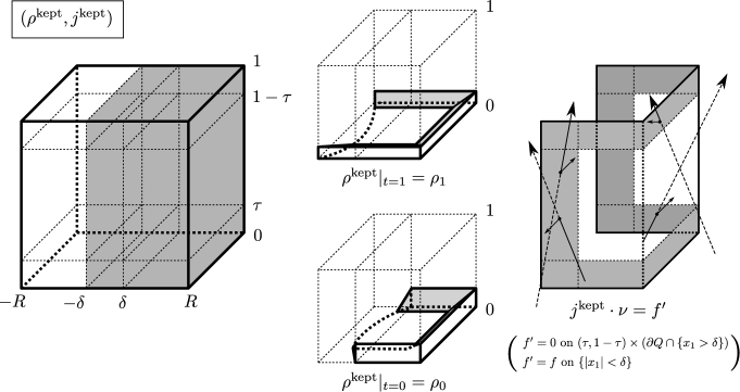
Figure 2. Kept trajectories $(\rho^{\mathrm{kept}},j^{\mathrm{kept}})$.

Step 4: Main construction. We now go into individual constructions, starting with the main construction. The main construction $(\rho^{\mathrm{main}},j^{\mathrm{main}})$ is defined by the sum of two measures $(\tilde{s},\tilde{q})$ and $(s,q)$ both living in $(\tau,1-\tau)\times(Q\cap\{x_{1}>\delta\})$. The former is defined by $(\tilde{s},\tilde{q}):=(\frac{t-\tau}{1-2\tau}c_{1}+\frac{1-\tau-t}{1-2\tau}c_{0},\frac{1}{1-2\tau}\nabla\tilde{\phi})$, cf. (5.27), which satisfies the continuity equation by (5.54), and connects the constant density $c_{0}$ at $t=\tau$ to the constant density $c_{1}$ at $t=1-\tau$, with constant-in-$t$ normal fluxes $\frac{1}{1-2\tau}\bar{g}$ across $(\tau,1-\tau)\times(Q\cap\{x_{1}=\delta\})$, cf. (5.28), and $\frac{1}{1-2\tau}\bar{f}$ across the remaining boundary portion $(\tau,1-\tau)\times(\partial Q\cap\{x_{1}>\delta\})$, cf. (5.24); its cost is directly computed as

$$\int_{(\tau,1-\tau)\times(Q\cap\{x_{1}>\delta\})}\frac{1}{\tilde{s}}|\tilde{q}|^{2}=\frac{1}{1-2\tau}\int_{0}^{1}\frac{dt}{tc_{1}+(1-t)c_{0}}\int_{Q\cap\{x_{1}>\delta\}}|\nabla\tilde{\phi}|^{2},$$

and hence by (5.55) and by $\int_{Q\cap\{x_{1}>\delta\}}|\nabla\tilde{\phi}|^{2}\lesssim E+\delta^{2}$ (e.g. from (5.37)) we have

(5.57) $$\int_{(\tau,1-\tau)\times(Q\cap\{x_{1}>\delta\})}\frac{1}{\tilde{s}}|\tilde{q}|^{2}-\int_{Q\cap\{x_{1}>\delta\}}|\nabla\tilde{\phi}|^{2}\lesssim(\tau+E^{\frac{1}{2}})(E+\delta^{2}).$$

The latter $(s,q)$ is based on the boundary layer construction from [16, Lemma 2.4]; it satisfies the continuity equation in $(\tau,1-\tau)\times(Q\cap\{x_{1}>\delta\})$ and $|s|\leq 1/2$, connects the zero-densities at $t=\tau$ and $t=1-\tau$, with no flux across $(\tau,1-\tau)\times(Q\cap\{x_{1}=\delta\})$ and flux $f^{\mathrm{main}}-\frac{1}{1-2\tau}\bar{f}$ across $(\tau,1-\tau)\times(\partial Q\cap\{x_{1}>\delta\})$, where $f^{\mathrm{main}}$ is defined (on $(0,1)\times\partial Q$ for later use) by

(5.58) $$f^{\mathrm{main}}:=\begin{cases}f-f^{\prime}+\frac{1}{1-2\tau}\int_{(0,\tau)\cup(1-\tau,1)}(f-f^{\prime})dt&\mbox{if}\ \tau<t<1-\tau,\\ 0&\mbox{else},\end{cases}$$

so that since $\int_{\tau}^{1-\tau}(f^{\mathrm{main}}-\frac{1}{1-2\tau}\bar{f})dt=0$ we may apply [16, Lemma 2.4]; in addition, noting that $\int_{\tau}^{1-\tau}(f^{\mathrm{main}}-\frac{1}{1-2\tau}\bar{f})^{2}dt\lesssim E$ by (5.24) and (5.35), we may choose $(s,q)$ to be concentrated on $(\tau,1-\tau)\times A_{r}$ for an $r\lesssim E^{\frac{1}{d+1}}\ll 1$, where $A_{r}:=Q\cap\{\mathrm{dist}(\cdot,\partial(Q\cap\{x_{1}>\delta\}))<r\}$, and also satisfy the key estimate

(5.59) $$\int_{(\tau,1-\tau)\times Q}|q|^{2}\lesssim\Big{(}\int_{(\tau,1-\tau)\times\partial Q}\big{(}f^{\mathrm{main}}-\frac{1}{1-2\tau}\bar{f}\big{)}^{2}\Big{)}^{\frac{d+2}{d+1}}\lesssim E^{\frac{d+2}{d+1}}.$$

In summary, $(\rho^{\mathrm{main}},j^{\mathrm{main}})$ connects the constant density $c_{0}$ at $t=\tau$ to the constant density $c_{1}$ at $t=1-\tau$, with fluxes $\frac{1}{1-2\tau}\bar{g}$ across $(\tau,1-\tau)\times(Q\cap\{x_{1}=\delta\})$ and $f^{\mathrm{main}}$ across $(\tau,1-\tau)\times(\partial Q\cap\{x_{1}>\delta\})$ (see Figure 3). By definition of $(\rho^{\mathrm{main}},j^{\mathrm{main}})$,

$$\int_{(0,1)\times\mathbb{R}^{d}}\frac{1}{\rho^{\mathrm{main}}}|j^{\mathrm{main}}|^{2} =\int_{(\tau,1-\tau)\times(Q\cap\{x_{1}>\delta\}\setminus A_{r})}\frac{1}{\tilde{s}}|\tilde{q}|^{2}+\int_{(\tau,1-\tau)\times A_{r}}\frac{1}{\tilde{s}+s}|\tilde{q}+q|^{2},$$

and hence by (5.57), by $|s|\leq 1/2$ and by $|\tilde{s}-1|\lesssim E^{\frac{1}{2}}\ll 1$, cf. (5.55),

$$\int_{(0,1)\times\mathbb{R}^{d}}\frac{1}{\rho^{\mathrm{main}}}|j^{\mathrm{main}}|^{2}-\int_{(\tau,1-\tau)\times(Q\cap\{x_{1}>\delta\})}\frac{1}{\tilde{s}}|\tilde{q}|^{2} \lesssim\int_{(\tau,1-\tau)\times A_{r}}(|\tilde{q}|^{2}+|q|^{2})$$

$$\lesssim\int_{A_{r}}|\nabla\tilde{\phi}|^{2}+E^{\frac{d+2}{d+1}}.$$

Combining this with (5.57) and $\int_{A_{r}}|\nabla\tilde{\phi}|^{2}\lesssim r(E+\delta^{2})$ (obtained by estimates such as (5.37) in all directions), recalling that $r\lesssim E^{\frac{1}{d+1}}$, and absorbing all the higher-order terms, we reach the desired

(5.60) $$\int_{(0,1)\times\mathbb{R}^{d}}\frac{1}{\rho^{\mathrm{main}}}|j^{\mathrm{main}}|^{2}-\int_{Q\cap\{x_{1}>\delta\}}|\nabla\tilde{\phi}|^{2}\lesssim\tau(E+\delta^{2})+(E+\delta^{2})^{\frac{d+2}{d+1}}.$$

Figure 3. Main construction.

Step 5: Singular construction. The singular construction $(\rho^{\mathrm{sing}},j^{\mathrm{sing}})$ is then taken for accommodating the flux $f^{\mathrm{main}}$ through $(0,1)\times\partial Q$, cf. (5.58), to the desired one $f-f^{\prime}$. More precisely, we define the measure $(\rho^{\mathrm{sing}},j^{\mathrm{sing}})$ concentrated on $(0,1)\times\partial Q$ (in fact on $(0,1)\times(\partial Q\cap\{x_{1}\geq\delta\})$) through the density

$$\rho^{\mathrm{sing}}:=\begin{cases}-\int_{0}^{t}(f-f^{\prime})&\mbox{for}\ t\in(0,\tau),\\ \frac{t+\tau-1}{1-2\tau}\int_{0}^{\tau}(f-f^{\prime})+\frac{t-\tau}{1-2\tau}\int_{1-\tau}^{1}(f-f^{\prime})&\mbox{for}\ t\in(\tau,1-\tau),\\ \int_{t}^{1}(f-f^{\prime})&\mbox{for}\ t\in(1-\tau,1),\end{cases}$$

which is made so that $\rho^{\mathrm{sing}}|_{t=0,1}=0$, $\rho^{\mathrm{sing}}\geq 0$, cf. (5.16), and $\partial_{t}\rho^{\mathrm{sing}}=f^{\mathrm{main}}-(f-f^{\prime})$ on $(0,1)\times\partial Q$ (see Figure 4). Then it distributionally solves the continuity equation with the everywhere-vanishing flux $j^{\mathrm{sing}}:=0$ in $(0,1)\times Q$, with flux $(f-f^{\prime})-f^{\mathrm{main}}$ across $(0,1)\times\partial Q$, so that this extra construction comes at no cost, cf. (4.18):

(5.61) $$\int_{(0,1)\times\mathbb{R}^{d}}\frac{1}{\rho^{\mathrm{sing}}}|j^{\mathrm{sing}}|^{2}=0.$$

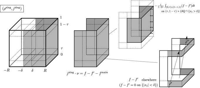
Figure 4. Singular construction.

Step 6: Boundary construction. We now turn to the boundary construction in $(\tau,1-\tau)\times(Q\cap\{x_{1}<\delta\})$; we recall that it connects the density $\chi_{\Omega_{0}\cap\{x_{1}<\delta\}}$ at $t=\tau$ to the density $\chi_{\Omega_{1}\cap\{x_{1}<\delta\}}$ at $t=1-\tau$, has constant-in-$t$ normal flux $-\frac{1}{1-2\tau}\bar{g}$ across $(\tau,1-\tau)\times(Q\cap\{x_{1}=\delta\})$, and no normal flux across $(\tau,1-\tau)\times(\partial Q\cap\{x_{1}<\delta\})$. The boundary construction is explicitly given by shearing in the normal direction $x_{1}$:

$$(\rho^{\mathrm{bdry}},j^{\mathrm{bdry}})(t,(x_{1},x^{\prime})):=\begin{cases}(1,-\frac{\bar{g}(x^{\prime})}{1-2\tau}e_{1})&\mbox{for}\ x_{1}>\frac{t-\tau}{1-2\tau}g_{1}(x^{\prime})+\frac{1-\tau-t}{1-2\tau}g_{0}(x^{\prime}),\\ (0,0)&\mbox{else},\end{cases}$$

which in view of the definition of $\bar{g}$, cf. (5.28), distributionally satisfies the continuity equation and obviously the desired flux boundary condition (see Figure 5). It satisfies the desired initial and terminal conditions by (4.3), and we have

(5.62) $$\int_{(0,1)\times\mathbb{R}^{d}}\frac{1}{\rho^{\mathrm{bdry}}}|j^{\mathrm{bdry}}|^{2}=\frac{1}{1-2\tau}\int_{Q^{\prime}}\big{(}\frac{g_{0}+g_{1}}{2}-\delta\big{)}\bar{g}^{2}\stackrel{{\scriptstyle\eqref{ao02}}}{{\lesssim}}\delta^{3}.$$

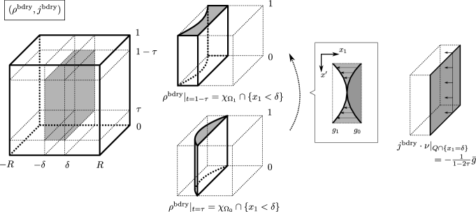
Figure 5. Boundary construction.

Step 7: Initial and terminal construction. The remainder of the proof is devoted to the initial and terminal construction; by symmetry, we restrict to the initial construction. The initial construction $(\rho^{\mathrm{ini}},j^{\mathrm{ini}})$ lives in $(0,\tau)\times Q$ and is defined by the (Eulerian) optimal transport from $(\chi_{\Omega_{0}}-\rho_{0})|_{Q}$ to $(\chi_{\Omega_{0}\cap\{x_{1}<\delta\}}+c_{0}\chi_{\{x_{1}>\delta\}})|_{Q}$ rescaled-in-$t$ from $(0,1)$ to $(0,\tau)$ (see Figure 6). The no-flux condition follows since $Q$ is convex. In what follows we will verify that

(5.63) $$\int_{(0,1)\times\mathbb{R}^{d}}\frac{1}{\rho^{\mathrm{ini}}}|j^{\mathrm{ini}}|^{2}\lesssim\big{(}\tau+\frac{(M+\delta)^{\frac{1}{d-1}}}{\tau}\big{)}E,$$

dividing the proof into Steps 7-1, 7-2, and 7-3.

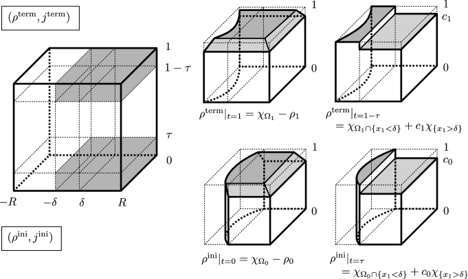
Figure 6. Initial and terminal construction.

Step 7-1: Estimate of the cost by using a Poisson equation. Estimate (5.63) is based on the following observation:

(5.64) $$\int_{(0,1)\times\mathbb{R}^{d}}\frac{1}{\rho^{\mathrm{ini}}}|j^{\mathrm{ini}}|^{2}\lesssim\frac{1}{\tau}\int_{\Omega_{0}}|\nabla\phi_{0}|^{2},$$

where $\nabla\phi_{0}$ solves the Neumann problem (solvable by (5.51)):

(5.65) $$\begin{cases}\Delta\phi_{0}=(1-c_{0})\chi_{\{x_{1}>\delta\}}-\rho_{0}&\mbox{in}\ \Omega_{0}\cap Q,\\ \nu\cdot\nabla\phi_{0}=0&\mbox{on}\ \partial(\Omega_{0}\cap Q).\end{cases}$$

Indeed, if $W_{Q}$ denotes the Wasserstein distance on the (convex) set $Q$, i.e., if for densities $\mu_{0}$ and $\mu_{1}$ of same mass on $Q$ we let $W_{Q}^{2}(\mu_{0},\mu_{1})$ denote the cost of the optimal transport map between $\mu_{0}|_{Q}$ and $\mu_{1}|_{Q}$, cf. (4.17), then by definition of the initial construction we have

(5.66) $$\int_{(0,1)\times\mathbb{R}^{d}}\frac{1}{\rho^{\mathrm{ini}}}|j^{\mathrm{ini}}|^{2}=\frac{1}{\tau}W_{Q}^{2}\big{(}\chi_{\Omega_{0}}-\rho_{0}\,,\,\chi_{\Omega_{0}\cap\{x_{1}<\delta\}}+c_{0}\chi_{\{x_{1}>\delta\}}\big{)}.$$

This entails (5.64) by two general observations: The first observation is that for arbitrary densities $\mu_{0}$, $\mu_{1}$ on $Q$ of the same mass we have

(5.67) $$W_{Q}(\mu_{0},\mu_{1})\leq\frac{1}{\sqrt{2}-1}W_{Q}(\mu_{0}+\mu_{1},2\mu_{1}).$$

Inequality (5.67) follows from the scaling of $W_{Q}$ in the mass, its triangle inequality, and its sub-additivity:

$$W_{Q}(\mu_{0},\mu_{1}) =\frac{1}{\sqrt{2}}W_{Q}(2\mu_{0},2\mu_{1})$$

$$\leq\frac{1}{\sqrt{2}}\big{(}W_{Q}(2\mu_{0},\mu_{0}+\mu_{1})+W_{Q}(\mu_{0}+\mu_{1},2\mu_{1})\big{)}$$

$$\leq\frac{1}{\sqrt{2}}\big{(}W_{Q}(\mu_{0},\mu_{1})+W_{Q}(\mu_{0}+\mu_{1},2\mu_{1})\big{)}.$$

The second observation is that for any smooth open set $\Omega_{0}$ and same generic densities $\mu_{0}$, $\mu_{1}$ (uniformly positive on $\Omega_{0}\cap Q$),

(5.68) $$W_{Q}^{2}(\mu_{0},\mu_{1})\leq\frac{1}{\inf_{\Omega_{0}\cap Q}\min\{\mu_{0},\mu_{1}\}}\int_{\Omega_{0}\cap Q}|\nabla\bar{\phi}|^{2},$$

where $\nabla\bar{\phi}$ solves the Neumann problem:

(5.69) $$\begin{cases}\Delta\bar{\phi}=\mu_{0}-\mu_{1}&\mbox{in}\ \Omega_{0}\cap Q,\\ \nu\cdot\nabla\bar{\phi}=0&\mbox{on}\ \partial(\Omega_{0}\cap Q).\end{cases}$$

This follows by appealing to the Eulerian formulation of the Wasserstein distance and choosing

$$(\bar{\rho},\bar{j})=\begin{cases}(t\mu_{1}+(1-t)\mu_{0},\nabla\bar{\phi})&\mbox{on}\ \Omega_{0}\cap Q,\\ (0,0)&\mbox{else},\end{cases}$$

so that the (distributional) continuity equation subject to $\bar{\rho}(0,\cdot)=\mu_{0}$ and $\bar{\rho}(1,\cdot)=\mu_{1}$ is a direct consequence of (5.69), and hence

$$W_{Q}^{2}(\mu_{0},\mu_{1})\leq\int_{(0,1)\times\mathbb{R}^{d}}\frac{1}{\bar{\rho}}|\bar{j}|^{2}.$$

Starting from (5.67) and applying (5.68) with $(\mu_{0},\mu_{1})$ replaced by $(\mu_{0}+\mu_{1},2\mu_{1})$ yield

$$W_{Q}^{2}(\mu_{0},\mu_{1})\leq\big{(}\frac{1}{\sqrt{2}-1}\big{)}^{2}\frac{1}{\inf_{\Omega_{0}\cap Q}\mu_{1}}\int_{\Omega_{0}\cap Q}|\nabla\bar{\phi}|^{2},$$

with $\bar{\phi}$ still defined as in (5.69), as long as $\mu_{0}$ and $\mu_{1}$ are supported on $\Omega_{0}\cap Q$ and of same mass there. Applying this to $\mu_{0}:=\chi_{\Omega_{0}}-\rho_{0}$ and $\mu_{1}:=\chi_{\Omega_{0}\cap\{x_{1}<\delta\}}+c_{0}\chi_{\{x_{1}>\delta\}}$ both restricted to $Q$, and hence $\phi_{0}$ playing the role of $\bar{\phi}$, we see that (5.66) turns into (5.64), where we also use (5.55).

Step 7-2: Elliptic estimates. In order to estimate the r.h.s. of (5.64), we need an elementary but perhaps somewhat un-usual elliptic estimate on (5.65), which capitalizes on the concentration of $\rho_{0}$ (which we extend trivially on $\mathbb{R}^{d}$) near $\partial Q$, namely

(5.70) $$\int_{Q\cap\Omega_{0}}|\nabla\phi_{0}|^{2}\lesssim\big{(}\int_{\partial Q}|\bar{\rho}_{0}|^{\frac{2(d-1)}{d}}\big{)}^{\frac{d}{d-1}}+\int_{Q}{\rm dist}^{2}(\cdot,\partial Q)\rho_{0}^{2},$$

where for any $x\in\partial Q$, $\bar{\rho}_{0}(x)$ is the integral of $|\rho_{0}|$ along the line perpendicular to $\partial Q$ in $x$ (non-negativity of $\rho_{0}$ is not needed for this linear estimate), more precisely, along the segment $I_{x}:=\{y\in Q\mid|y-x|={\rm dist}(y,\partial Q)\}$, i.e., consisting of those points that have $x$ as their (orthogonal) projection onto $\partial Q$. In case of $d=2$, the exponent $\frac{2(d-1)}{d}$, which would be $=1$, has to be replaced by an (in fact, any) exponent $q>1$. For later reference we retain the elementary inequality

(5.71) $$\frac{1}{2}\bar{\rho}_{0}(x)^{2}\leq\sup_{I_{x}}|\rho_{0}|\int_{I_{x}}{\rm dist}(\cdot,\partial Q)|\rho_{0}|.$$

For the convenience of the reader, we give the argument for (5.71) (for general $\rho_{0}$): Writing $\rho_{0}=|\rho_{0}|$, we may assume $\rho_{0}\geq 0$; by homogeneity, we may assume $\sup_{I_{x}}\rho_{0}=1$. By an extremality argument we may then assume $\rho_{0}\in\{0,1\}$, so that we are dealing with a characteristic function of a subset of $I_{x}$. It is clear that the configuration that minimizes $\int_{I_{x}}{\rm dist}(\cdot,\partial Q)\rho_{0}$ comes from an interval adjacent to the boundary of $I_{x}$, so that (5.71) follows from an explicit calculation.

We now turn to the argument for (5.70): Since we may without loss of generality assume that $\int_{Q\cap\{x_{1}>\delta\}}\phi_{0}$ $=0$, we obtain from testing (5.65):

$$\int_{Q\cap\Omega_{0}}|\nabla\phi_{0}|^{2}=\int_{Q\cap\Omega_{0}}\phi_{0}\rho_{0}.$$

It is convenient to have an extension $\zeta$ of $\phi_{0}$ on all of $\mathbb{R}^{d}$, but supported in $2Q$, at hand with $\int_{\mathbb{R}^{d}}|\nabla\zeta|^{2}\lesssim\int_{Q\cap\Omega_{0}}|\nabla\phi_{0}|^{2}$, which exists since $Q\cap\partial\Omega_{0}$ is in particular locally a Lipschitz graph with constant $\leq 1$. Hence it suffices to establish

$$\big{|}\int_{\mathbb{R}^{d}}\zeta\rho_{0}\big{|}^{2}\lesssim\Big{(}\big{(}\int_{\partial Q}|\bar{\rho}_{0}|^{\frac{2(d-1)}{d}}\big{)}^{\frac{d}{d-1}}+\int_{Q}{\rm dist}^{2}(\cdot,\partial Q)\rho_{0}^{2}\Big{)}\int_{\mathbb{R}^{d}}|\nabla\zeta|^{2},$$

which amounts to an estimate of $\rho_{0}$ in $H^{-1}$. For this, it is convenient to split the cube $Q$ into $2d$ pyramids consisting of those points closest to one of the faces; we split $\rho_{0}$ into $2d$ pieces $\rho$ accordingly. Hence it is enough to replace $Q$ by the half space $\{(x_{1},x^{\prime})\mid x_{1}>0\}$:

$$\big{|}\int_{\{x_{1}>0\}}\zeta\rho\big{|}^{2}\lesssim\Big{(}\big{(}\int_{\mathbb{R}^{d-1}}|\bar{\rho}|^{\frac{2(d-1)}{d}}\big{)}^{\frac{d}{d-1}}+\int_{\{x_{1}>0\}}x_{1}^{2}\rho^{2}\Big{)}\int_{\mathbb{R}^{d}}|\nabla\zeta|^{2},$$

where the bar still denotes the integral in normal direction, which now means $\bar{\rho}(x^{\prime})=\int_{0}^{\infty}\rho(x_{1},x^{\prime})dx_{1}$. This is best seen by splitting the l.h.s. as

$$\int_{\{x_{1}>0\}}\zeta\rho=\int_{\mathbb{R}^{d-1}}\zeta(0,\cdot)\bar{\rho}+\int_{\{x_{1}>0\}}(\zeta-\zeta(0,\cdot))\rho.$$

The first r.h.s. term is estimated as desired by Hölder’s inequality and by the Sobolev trace inequality on $\zeta$ in form of $\big{(}\int_{\mathbb{R}^{d-1}}|\zeta(0,\cdot)|^{\frac{2(d-1)}{d-2}})^{\frac{d-2}{2(d-1)}}$ $\lesssim(\int_{\mathbb{R}^{d}}|\nabla\zeta|^{2})^{\frac{1}{2}}$; in the case of $d=2$ we use that for any $p<\infty$, $\big{(}\int_{\mathbb{R}^{d-1}}|\zeta(0,\cdot)|^{p})^{\frac{1}{p}}$ $\lesssim(\int_{\mathbb{R}^{d}}|\nabla\zeta|^{2})^{\frac{1}{2}}$, making use of the fact that $\zeta$ is supported in $2Q$. The second r.h.s. term can be rewritten as

$$\int_{\{x_{1}>0\}}(\zeta-\zeta(0,\cdot))\rho=\int_{\{x_{1}>0\}}\rho\int_{0}^{x_{1}}\partial_{1}\zeta=\int_{\{x_{1}>0\}}\partial_{1}\zeta\int_{x_{1}}^{\infty}\rho,$$

so that the desired estimate follows from the Cauchy-Schwarz inequality on $\{x_{1}>0\}$ and Hardy’s inequality in form of

$$\int_{0}^{\infty}\big{(}\int_{x_{1}}^{\infty}\rho\big{)}^{2}dx_{1}\leq 4\int_{0}^{\infty}x_{1}^{2}\rho^{2}dx_{1}.$$

Step 7-3: Completion of the estimate for the initial construction. Equipped with (5.70), we are now in a position to prove (5.63). The second contribution to (5.70) is easily estimated: By the $L^{\infty}$-bound (5.32) in conjunction with definition (5.14) and ${\mathcal{T}}_{+}^{\prime}$ $\subset{\mathcal{T}}_{+}$ we have

$${\rm supp}\rho_{0}\subset\{{\rm dist}(\cdot,\partial Q)\leq M\}.$$

Combining this with (5.21), we have

$$\int_{Q}{\rm dist}^{2}(\cdot,\partial Q)\rho_{0}^{2}\lesssim ME.$$

The first contribution in (5.70) requires more care; we split $\rho_{0}$ into $\rho_{0}^{\prime}$ and $\rho_{0}-\rho_{0}^{\prime}$, cf. (5.18). On the contribution from $\rho_{0}^{\prime}$, or rather its integral $\bar{\rho}_{0}^{\prime}$ in the normal direction to $\partial Q$ (defined as the above $\bar{\rho}_{0}$), we use Hölder’s inequality:

$$\big{(}\int_{\partial Q}(\bar{\rho}_{0}^{\prime})^{\frac{2(d-1)}{d}}\big{)}^{\frac{d}{d-1}}\lesssim\int_{\partial Q}(\bar{\rho}_{0}^{\prime})^{2}\stackrel{{\scriptstyle\eqref{ao29}}}{{\lesssim}}\sup|\rho_{0}^{\prime}|\int_{Q}{\rm dist}(\cdot,\partial Q)|\rho_{0}^{\prime}|\stackrel{{\scriptstyle\eqref{ao46}}}{{\lesssim}}\tau^{2}E.$$

We now turn to the contribution from $\rho_{0}-\rho_{0}^{\prime}$ and note that by definitions (5.14) and (5.18), we have

$$\begin{split}\int\zeta(\rho_{0}-\rho_{0}^{\prime})=\int_{{\mathcal{T}}_{+}^{\prime}\setminus{\mathcal{T}}_{+}^{\prime\prime}}\zeta(X(0))\mathbb{P}(dX),\\ \mbox{with}\quad{\mathcal{T}}_{+}^{\prime}\setminus{\mathcal{T}}_{+}^{\prime\prime}\subset\{X\in{\mathcal{T}}_{+}\mid|X_{1}(t_{+})|<\delta\},\end{split}$$

so that by the $L^{\infty}$-bound (5.32) we obtain

$$\begin{array}[]{c}{\rm supp}(\rho_{0}-\rho_{0}^{\prime})\subset\{|x_{1}|\leq M+\delta\}\cap\{{\rm dist}(\cdot,\partial Q)\leq M\}\\[4.30554pt] \mbox{and thus}\quad{\rm supp}(\overline{\rho_{0}-\rho_{0}^{\prime}})\subset\{|x_{1}|\leq M+\delta\},\end{array}$$

where $\overline{\rho_{0}-\rho_{0}^{\prime}}$ denotes the integral of $\rho_{0}-\rho_{0}^{\prime}$ in the normal direction (as above). This allows us to use Hölder’s inequality in the following form

$$\big{(}\int_{\partial Q}\overline{\rho_{0}-\rho_{0}^{\prime}}^{\frac{2(d-1)}{d}}\big{)}^{\frac{d}{d-1}}\lesssim(M+\delta)^{\frac{1}{d-1}}\int_{\partial Q}\overline{\rho_{0}-\rho_{0}^{\prime}}^{2}$$

$$\leq(M+\delta)^{\frac{1}{d-1}}\int_{\partial Q}\bar{\rho}_{0}^{2}\stackrel{{\scriptstyle\eqref{ao29},\eqref{ao44}}}{{\lesssim}}(M+\delta)^{\frac{1}{d-1}}E.$$

Combining all three contributions we obtain

$$\int_{Q\cap\Omega_{0}}|\nabla\phi_{0}|^{2}\lesssim(\tau^{2}+(M+\delta)^{\frac{1}{d-1}})E,$$

which in turn we insert in (5.64) to end up with (5.63).

Finally, we notice that the local competitor $(\tilde{\rho},\tilde{j})$ of the form (5.4) is admissible in the sense of (5.10), and then deduce (5.4) from (5.56), (5.60), (5.61), (5.62) and (5.63) combined with sub-additivity, completing the proof. ∎

6. From harmonic approximation to $C^{1,\alpha}$-regularity

In this final section we complete the proof of Theorem 1.1, demonstrating that the harmonic approximation of Proposition 4.1 implies the boundary $C^{1,\alpha}$-regularity via the steps in Section 2. Throughout this section we use the same notations as in Section 2.

6.1. One-step improvement result

Proof of Proposition 2.4.

Fix any $\Omega_{0}$, $\Omega_{1}$, $T$, and $R$ satisfying the conditions. Without loss of generality we may assume that $\nu_{0}(0)=-e_{1}$ $(=\nu_{1}(0))$ by rotation. In what follows we fix $\beta\in(0,1)$ and always implicitly assume that $E+D\ll_{\beta}1$ (and hence $E+D\ll 1$ in particular). In addition, we use the same notation $C>0$ for all universal constants depending only on $d$ and $\alpha$.

Step 1: Definition of $b$ and $B$. We define $\bar{b}\in\mathbb{R}^{d}$ and $\bar{A},\bar{B}\in\mathbb{R}^{d\times d}$ by

(6.1) $$\bar{b}:=\nabla\phi(0),\quad\bar{A}:=\nabla^{2}\phi(0),\quad\bar{B}:=e^{-\bar{A}/2},$$

where $\phi$ is as in Proposition 2.3. Notice that $\bar{B}$ is symmetric, i.e., $\bar{B}=\bar{B}^{*}$ since so is $\bar{A}$. By the mean value property of harmonic $\nabla\phi$,

(6.2) $$|\bar{b}|^{2}+|\bar{A}|^{2}=|\nabla\phi(0)|^{2}+|\nabla^{2}\phi(0)|^{2}\lesssim\int_{B_{r}}|\nabla\phi|^{2}\stackrel{{\scriptstyle\eqref{eqn:harmonicDirichlet}}}{{\lesssim}}E,$$

and thus in particular $|\bar{A}|\ll 1$ so that $|\bar{B}-Id|^{2}\lesssim|\bar{A}|^{2}\lesssim E$; hence,

(6.3) $$|\bar{b}|^{2}+|\bar{B}-Id|^{2}\lesssim E\ll 1.$$

In addition, $\bar{b}\cdot e_{1}=0$, i.e., $\bar{b}$ is perpendicular to $e_{1}$, and moreover $\bar{B}$ has the block structure of $\bar{B}_{i1}=\bar{B}_{1j}=0$ for $i,j\geq 2$, where $\bar{B}=(\bar{B}_{ij})$. Indeed, $\partial_{1}\phi(0,x^{\prime})=0$ holds for all $(0,x^{\prime})\in B_{r}$ by the reflection symmetry (2.7). Hence, $\partial_{1}\phi(0)=0$ so that $\bar{b}\cdot e_{1}=0$, cf. (6.1), and also $\nabla^{\prime}\partial_{1}\phi(0)=0$ so that $\bar{A}$ has the desired block structure, from which $\bar{B}$ inherits the same block structure.

We will see later (in Step 3) that an affine transformation defined by $\bar{b}$ and $\bar{B}$ plays a key role in proving the main estimate (2.11) as in the interior regularity theory. However this transformation generically destroys the well-preparedness of the boundaries. In order to recover the well-preparedness we need to modify $\bar{b}$ and $\bar{B}$ to $b$ and $B$ so that not only (2.10) still holds but also, for later use, the deviation $|B-\bar{B}|^{2}+|b-\bar{b}|^{2}$ is super-linearly bounded by $E+D$.

We first define $b$ by

(6.4) $$b:=\bar{b}+\widetilde{b},$$

taking a vector $\widetilde{b}$ of the form $\ell e_{1}$ so that $0\in\partial\Omega_{0}\cap\partial(\Omega_{1}-b)$; namely, we take $\ell:=g_{1}(\bar{b}^{\prime})$, where $g_{1}$ denotes the graph representation of $\partial\Omega_{1}$ near the origin, and $\bar{b}^{\prime}\in\mathbb{R}^{d-1}$ denotes the last $(d-1)$-components of $\bar{b}$. Then we have the super-linear estimate

(6.5) $$|\widetilde{b}|^{2}=|g_{1}(\bar{b}^{\prime})|^{2}\leq([\nabla^{\prime}g_{1}]_{\alpha,B_{1}}|\bar{b}|^{1+\alpha})^{2}\stackrel{{\scriptstyle\eqref{ao014}}}{{\lesssim}}DE^{1+\alpha}\leq(E+D)^{2+\alpha},$$

and, since $|b|^{2}=|\bar{b}|^{2}+|\widetilde{b}|^{2}$, we get in particular

(6.6) $$|b|^{2}\lesssim E+D.$$

We then define $B$ by

(6.7) $$B:=\widetilde{B}\bar{B},$$

seeking a certain matrix $\widetilde{B}$ to make the normals of $\hat{\Omega}_{0}$ ($=B^{-*}\Omega_{0}$) and $\hat{\Omega}_{1}$ ($=B(\Omega_{1}-b)$) at the origin parallel in the following way. Since the normals are transformed by the cofactor matrices under affine changes of variables, the normals of $\bar{B}(\Omega_{1}-b)$ and $\bar{B}^{-*}\Omega_{0}$ are parallel to $\bar{B}^{-*}\nu_{1}(b)$ and $\bar{B}\nu_{0}(0)$, respectively, and thus in general not parallel to each other. Note however that because of the above-mentioned block structure of $\bar{B}$ and the well-preparedness, $\bar{B}^{-*}\nu_{1}(0)=-\bar{B}^{-*}e_{1}$ and $\bar{B}\nu_{0}(0)=-\bar{B}e_{1}$ are parallel to $-e_{1}$, so that

$$\Big{|}\frac{\bar{B}^{-*}\nu_{1}(b)}{|\bar{B}^{-*}\nu_{1}(b)|}-\frac{\bar{B}\nu_{0}(0)}{|\bar{B}\nu_{0}(0)|}\Big{|}^{2}=\Big{|}\frac{\bar{B}^{-*}\nu_{1}(b)}{|\bar{B}^{-*}\nu_{1}(b)|}-\frac{\bar{B}^{-*}\nu_{1}(0)}{|\bar{B}^{-*}\nu_{1}(0)|}\Big{|}^{2}$$

(6.8) $$\stackrel{{\scriptstyle\eqref{ao014}}}{{\lesssim}}|\nu_{1}(b)-\nu_{1}(0)|^{2}\lesssim([\nabla^{\prime}g_{1}]_{\alpha,1}|b|^{\alpha})^{2}\stackrel{{\scriptstyle\eqref{eqn:onestep10}}}{{\lesssim}}D(E+D)^{\alpha}.$$

Hence it suffices to find some matrix $\widetilde{B}$ such that $\widetilde{B}^{-*}\bar{B}^{-*}\nu_{1}(b)$ ($=B^{-*}\nu_{1}(b)$) and $\widetilde{B}\bar{B}\nu_{0}(0)$ (=$B\nu_{0}(0)$) are parallel, and that is close to the identity in the super-linear sense of

(6.9) $$|\widetilde{B}-Id|^{2}\lesssim(E+D)^{1+\alpha}.$$

We restrict ourselves to constructing a matrix $\widetilde{B}$, the square $\widetilde{A}:=\widetilde{B}^{2}$ of which is symmetric and to satisfy $\widetilde{A}\frac{\bar{B}\nu_{0}(0)}{|\bar{B}\nu_{0}(0)|}=\frac{\bar{B}^{-*}\nu_{1}(b)}{|\bar{B}^{-*}\nu_{1}(b)|}$. Since within the space of symmetric matrices, in a small neighborhood of the identity matrix, the square root is well defined and a Lipschitz operation, for (6.9) it is enough to construct such a symmetric matrix with $|\widetilde{A}-Id|^{2}\lesssim(E+D)^{1+\alpha}$. This is easily done: We think of $\mathbb{R}^{d}$ as orthogonal sum of the space spanned by $\frac{\bar{B}\nu_{0}(0)}{|\bar{B}\nu_{0}(0)|}=-e_{1}$ and its complement, and of $\widetilde{A}$ as a corresponding symmetric block matrix: On the one-dimensional space, $\widetilde{A}$ is defined as required, which by symmetry determines $\widetilde{A}$ up to the $(d-1)$-dimensional diagonal block, where $\widetilde{A}$ is set to be the identity: Since $|\widetilde{A}e_{1}-e_{1}|^{2}\lesssim D(E+D)^{\alpha}$ by (6.8), this closeness to the identity translates to the entire matrix $\widetilde{A}$. We deduce from (6.3) and (6.9) that $|B-Id|^{2}\lesssim E+D$, which together with (6.6) implies (2.10).

Step 2: Well-preparedness of $\hat{T}$. The optimality of $\hat{T}$ follows from the general affine invariance. We also have $\hat{\lambda}=\lambda|\det B|^{-2}\in[1/4,4]$ since $|\lambda-1|^{2}\lesssim E\ll 1$ by Lemma 4.2 and since $||\det B|-1|^{2}\lesssim|B-Id|^{2}\lesssim E+D\ll 1$ by (2.10). In addition, by definition of $B$ and $b$ in Step 1, the open sets $\hat{\Omega}_{0}$ and $\hat{\Omega}_{1}$ satisfy the tangency condition (1.2) at the origin, and moreover for any fixed $\theta\in(0,1/2)$ (which we will fix later) the topological condition (1.3) holds in $B_{\theta}$ by the $L^{\infty}$-bounds in Proposition 2.2, provided that $E+D\ll_{\theta}1$; this smallness will be satisfied since $E+D\ll_{\beta}1$ and $\theta$ will only depend on $\beta$ (next to $d$, $\alpha$).

Step 3: Estimate for $\hat{E}$. We now prove the main estimate (2.11), provided that $E+D\ll_{\theta}1$ for a given $\theta\in(0,r/4)$ which we fix later, where $r$ denotes the radius in Proposition 2.3. By $|B-Id|\ll_{\theta}1$, cf. (2.10), we in particular have $|B|\lesssim 1$, $|\det B^{-*}|\lesssim 1$ and $B^{*}(B_{\theta})\subset B_{2\theta}$; hence,

$$\hat{E} =\frac{1}{\theta^{2}|B_{\theta}|}\int_{B_{\theta}}|\hat{T}-\hat{x}|^{2}\chi_{\hat{\Omega}_{0}}$$

$$\lesssim\theta^{-(d+2)}\int_{B^{*}(B_{\theta}\cap\hat{\Omega}_{0})}|B(T-b)-B^{-*}x|^{2}|\det B^{-*}|$$

$$\lesssim\theta^{-(d+2)}\int_{B_{2\theta}\cap\Omega_{0}}|T-b-(B^{*}B)^{-1}x|^{2}.$$

In view of the triangle inequality this is bounded above by

$$\theta^{-(d+2)}\int_{B_{2\theta}\cap\Omega_{0}}(|T-x-\nabla\phi|^{2}+|\nabla\phi-\bar{b}-\bar{A}x|^{2}$$

(6.10) $$\qquad\qquad+|x+\bar{A}x-\bar{B}^{-2}x|^{2}+|\bar{B}^{-2}x-(B^{*}B)^{-1}x|^{2}+|\bar{b}-b|^{2}).$$

We now estimate these five terms. By Proposition 2.3, for any $\varepsilon\in(0,1)$, if $E+D\ll_{\varepsilon}1$, the first term is bounded as

$$\theta^{-(d+2)}\int_{B_{2\theta}\cap\Omega_{0}}|T-x-\nabla\phi|^{2}\lesssim\theta^{-(d+2)}(\varepsilon E+\frac{1}{\varepsilon}D),$$

since $B_{2\theta}\subset B_{r}$. Next, in view of the definition (6.1), by Taylor’s estimate the second term is bounded as

$$\theta^{-(d+2)}\int_{B_{2\theta}\cap\Omega_{0}}|\nabla\phi-\bar{b}-\bar{A}x|^{2}\lesssim\theta^{-(d+2)}\sup_{B_{2\theta}}|\nabla^{3}\phi|^{2}\int_{B_{2\theta}\cap\Omega_{0}}|x|^{4}\lesssim\theta^{2}E,$$

where in the last estimate, noting that $B_{2\theta}\subset B_{r/2}$, we again used the mean-value property and (2.6) for obtaining $\sup_{B_{2\theta}}|\nabla^{3}\phi|^{2}\lesssim\int_{B_{r}}|\nabla\phi|^{2}\lesssim E$. The third term is bounded as

$$\theta^{-(d+2)}\int_{B_{2\theta}\cap\Omega_{0}}|x+\bar{A}x-\bar{B}^{-2}x|^{2}\lesssim\theta^{-(d+2)}\int_{B_{2\theta}\cap\Omega_{0}}|\bar{A}|^{4}|x|^{2}\lesssim E^{2},$$

because $|\bar{A}|^{2}\lesssim E\ll 1$ by (6.2) and hence $|Id+\bar{A}-\bar{B}^{-2}|=|e^{\bar{A}}-Id-\bar{A}|\lesssim|\bar{A}|^{2}$. Concerning the fourth term, noting that all the matrices are regular and their norms are comparable to $1$, cf. (2.10), (6.3), and (6.9), we obtain the bound that

$$\theta^{-(d+2)}\int_{B_{2\theta}\cap\Omega_{0}}|\bar{B}^{-2}x-(B^{*}B)^{-1}x|^{2} \lesssim|\bar{B}^{-2}-(B^{*}B)^{-1}|^{2}\lesssim|B^{*}B-\bar{B}^{2}|^{2}$$

$$\stackrel{{\scriptstyle\eqref{ao017}}}{{\lesssim}}|\widetilde{B}-Id|^{2}\stackrel{{\scriptstyle\eqref{eqn:onestep5}}}{{\lesssim}}(E+D)^{1+\alpha}.$$

Finally, the fifth term is bounded as

$$\theta^{-(d+2)}\int_{B_{2\theta}\cap\Omega_{0}}|\bar{b}-b|^{2}\stackrel{{\scriptstyle\eqref{ao018}}}{{\lesssim}}\theta^{-2}|\tilde{b}|^{2}\stackrel{{\scriptstyle\eqref{eqn:onestep4}}}{{\lesssim}}\theta^{-2}(E+D)^{2+\alpha}.$$

In summary, keeping the linear terms with respect to $E$ and $D$ and absorbing all super-linear terms into the one with the smallest exponent $(E+D)^{1+\alpha}$, we find that for any $\theta\in(0,r/4)$, if $E+D\ll_{\theta,\varepsilon}1$, then there is $\bar{C}=\bar{C}(d,\alpha)>0$ such that

$$\hat{E}=\theta^{-2}\fint_{B_{\theta}}|\hat{T}-\hat{x}|^{2}\chi_{\hat{\Omega}_{0}}\leq\bar{C}\big{(}(\varepsilon\theta^{-(d+2)}+\theta^{2})E+\varepsilon^{-1}\theta^{-(d+2)}D+(E+D)^{1+\alpha}\big{)}.$$

Now, we fix $\theta\ll_{\beta}1$ so small that $\bar{C}\theta^{2}\leq\frac{1}{3}\theta^{2\beta}$; this is possible since $\beta<1$. Next, we fix $\varepsilon\ll_{\beta}1$ so small that $\bar{C}\varepsilon\theta^{-(d+2)}\leq\frac{1}{3}\theta^{2\beta}$. Finally, thanks to $E+D\ll_{\beta}1$, we have

$$\bar{C}(E+D)^{1+\alpha}\leq\frac{1}{3}\theta^{2\beta}(E+D),$$

and thus we conclude that if $E+D\ll_{\beta}1$, then

$$\hat{E}=\theta^{-2}\fint_{B_{\theta}}|\hat{T}-\hat{x}|^{2}\chi_{\hat{\Omega}_{0}} \leq\theta^{2\beta}E+C_{\beta}D,$$

which implies (2.11) since $\theta$ and $\varepsilon$ only depend on $\beta$ (and $d$, $\alpha$).

Step 4: Estimate for $\hat{D}$. Finally we prove (2.12). By definition, this amounts to show that for $i=0,1$,

(6.11) $$[\hat{\nu}_{i}]_{\alpha,B_{\theta}}\leq(1+C\sqrt{E+D})[\nu_{i}]_{\alpha,B_{1}},$$

where $\nu_{i}$ and $\hat{\nu}_{i}$ respectively denote the outer unit normal vectors of $\partial\Omega_{i}$ and $\partial\hat{\Omega}_{i}$.

We prove (6.11) only for $i=0$; the case $i=1$ is similar since the translation by $b$ does not change the Hölder semi-norm of the boundary (up to which part of the boundary is monitored). For notational simplicity, let $\hat{B}:=B^{-*}$. Since $|\hat{B}-Id|$ and $\theta$ are small, for any $\hat{x},\hat{y}\in\partial\hat{\Omega}_{0}\cap B_{\theta}$ there are unique points $x,y\in\partial\Omega_{0}\cap B_{1}$, respectively, such that $\hat{x}=\hat{B}x$ and $\hat{y}=\hat{B}y$. For such points we have

$$|\hat{x}-\hat{y}|^{-\alpha}\leq(1+C\sqrt{E+D})|x-y|^{-\alpha},$$

since

$$|x-y|\leq|B^{*}||\hat{x}-\hat{y}|\leq(1+C\sqrt{E+D})|\hat{x}-\hat{y}|.$$

Thus (6.11) is reduced to showing

$$\Big{|}\frac{\hat{B}\nu_{0}(x)}{|\hat{B}\nu_{0}(x)|}-\frac{\hat{B}\nu_{0}(y)}{|\hat{B}\nu_{0}(y)|}\Big{|}\leq(1+C|\hat{B}-Id|)|\nu_{0}(x)-\nu_{0}(y)|,$$

which by the triangle inequality follows from

$$\Big{|}\big{(}\frac{\hat{B}\nu_{0}(x)}{|\hat{B}\nu_{0}(x)|}-\nu_{0}(x)\big{)}-\big{(}\frac{\hat{B}\nu_{0}(y)}{|\hat{B}\nu_{0}(y)|}-\nu_{0}(y)\big{)}\Big{|}\lesssim|\hat{B}-Id||\nu_{0}(x)-\nu_{0}(y)|.$$

This amounts to the statement that the mapping

$$\hat{B}\mapsto\big{(}\partial B\ni\nu\mapsto\frac{\hat{B}\nu}{|\hat{B}\nu|}\in\partial B\big{)}$$

is Lipschitz continuous from a neighborhood of $Id$ with values in the Lipschitz transformations of the sphere $\partial B$. The latter is a direct consequence of the (local) smoothness of $(\hat{B},\nu)\mapsto\frac{\hat{B}\nu}{|\hat{B}\nu|}$ and the compactness of $\partial B$. ∎

Remark 6.1.

We now briefly explain why we have to allow the values of the initial and target densities to be different. The main reason is to obtain a super-linear type estimate in Step 3 of the above proof. In fact, if we had only allowed $\lambda=\hat{\lambda}=1$ in (2.8), then in order to get the marginal condition $\hat{T}\sharp\chi_{\hat{\Omega}_{0}}=\chi_{\hat{\Omega}_{1}}$, we need to take $\hat{T}(\hat{x})=\hat{c}B(T(B^{*}\hat{x})-b)$ with $\hat{c}:=|\det B|^{-2/d}$ (and $\hat{\Omega}_{1}=\hat{c}B(\Omega_{1}-b)$). In this case we need to replace the fourth term $|\bar{B}^{-2}x-(B^{*}B)^{-1}x|^{2}$ in (6.10) by $|\bar{B}^{-2}x-(\hat{c}B^{*}B)^{-1}x|^{2}$, and thus the super-linear bound of the form $\lesssim(E+D)^{1+\alpha}$ deteriorates into a linear bound $\lesssim E+D$, since we only have $|\hat{c}-1|^{2}\lesssim|\det B-1|^{2}\lesssim|B-Id|^{2}\lesssim E$. The linear bound is not sufficient for our purpose.

Remark 6.2.

Here is also a good position to observe that the (qualitative) tangency condition (1.2) is not restrictive; more precisely, we need not assume $p\in\partial\Omega_{0}\cap\partial\Omega_{1}$ and $\nu_{0}(p)=\nu_{1}(p)$ if we instead assume a natural quantitative counterpart. To observe this fact, for notational simplicity, we may suppose that $\Omega_{0}$ and $\Omega_{1}$ are represented by the epigraphs of $g_{0},g_{1}\in C^{1,\alpha}$ in the $e_{1}$-direction locally in the unit ball $B_{1}$ (i.e., $p=0$ and $R=1$), respectively, and also $g_{0}(0)=0$ and $\nabla^{\prime}g_{0}(0)=0$ (but $g_{1}$ is not qualitatively fixed). Now, we assume that in addition to $E\ll 1$,

$$\widetilde{D}:=|g_{1}(0)|^{2}+|\nabla^{\prime}g_{1}(0)|^{2}+[\nabla^{\prime}g_{0}]_{\alpha}^{2}+[\nabla^{\prime}g_{1}]_{\alpha}^{2}\ll 1,$$

where the first two terms yield the natural “quantitative” tangency condition (while the last two correspond to the original $D$). Then in particular $|\nu_{1}(0)-\nu_{0}(0)|^{2}\lesssim|\nabla^{\prime}g_{1}(0)|^{2}\ll 1$, so that there is a symmetric positive definite matrix $A$ such that $A\nu_{0}(0)=\nu_{1}(0)$ and $|A-Id|^{2}\lesssim|\nabla^{\prime}g_{1}(0)|^{2}\ll 1$ (see the last part of Step 1 above). Then the transformed map $\hat{T}$ defined in (2.8) with $B:=A^{\frac{1}{2}}$ and $b=g_{1}(0)e_{1}$ satisfies the assumption of Theorem 1.1 (including the tangency condition) at least in a (slightly) smaller ball, so that the desired assertion holds in a smaller ball. This can be translated back to the original map in a similar way, where all the terms in $\widetilde{D}$ also appear in the r.h.s. of the last linear estimate in Theorem 1.1.

6.2. Iteration

For convenience of the readers we give a complete proof, which is however almost parallel to a part of the proof of [16, Proposition 3.7],

Proof of Proposition 2.5.

The assertions (2.13) and (2.14) follow if we prove the following discrete version: For any nonnegative integer $k$ there are $\bar{A}_{k}$ and $\bar{a}_{k}$ such that

(6.12) $$\frac{1}{(\frac{1}{2}\theta^{k})^{d+2+2\alpha}}\int_{B_{\frac{1}{2}\theta^{k}}}|T-(\bar{A}_{k}x+\bar{a}_{k})|^{2}\chi_{\Omega_{0}}\lesssim E+D,$$

and

(6.13) $$|\bar{A}_{k}-Id|^{2}+\frac{1}{\theta^{2k}}|\bar{a}_{k}|^{2}\lesssim E+D,$$

where $\theta\in(0,1)$ is the constant in Proposition 2.4. In what follows we prove this discrete version by using Proposition 2.4 iteratively.

Step 1: Inductive argument for iteration via the one-step improvement. Set $\Omega_{0,0}:=\Omega_{0}$, $\Omega_{1,0}:=\Omega_{1}$, $T_{0}:=T$, $\lambda_{0}=\lambda$. We demonstrate that we can inductively define $\Omega_{0,k}$, $\Omega_{1,k}$, $T_{k}$, $\lambda_{k}$, $B_{k}$, $b_{k}$ by applying Proposition 2.4 to $\Omega_{0,{k-1}}$, $\Omega_{1,{k-1}}$, $\lambda_{k-1}$, $T_{k-1}$ with the exponent $\beta:=(\alpha+1)/2>\alpha$; now all constants depending on $\beta$ are universal (i.e., only depending on $d$ and $\alpha$). Notice carefully that for this inductive definition we need to inductively verify the smallness hypothesis (2.9) for all $k$.

We now verify by induction that for all $k$ we have not only the hypothesis (2.9) but also the stronger key estimate

(6.14) $$E_{k}+D_{k}\leq C^{\prime}\theta^{2\alpha k}(E+D)\ (\ll 1),$$

where $E_{k}:=E(\Omega_{0,k},\Omega_{0,k},T_{k},\theta^{k})$, $D_{k}:=D(\Omega_{0,k},\Omega_{0,k},\theta^{k})$, and $C^{\prime}=C^{\prime}(d,\alpha)\in[1,\infty)$ is defined by

$$C^{\prime}:=C_{1}^{\prime}+C_{2}^{\prime}\quad\textrm{with}\quad C_{1}^{\prime}:=\bar{C}\theta^{-2\beta}\sup_{k\geq 1}\big{(}k\theta^{2(\beta-\alpha)(k-1)}\big{)},\quad C_{2}^{\prime}:=\prod_{k=1}^{\infty}(1+\theta^{\alpha k}),$$

and $\bar{C}:=\max\{C_{\beta},C\}$ for $C_{\beta}$ in (2.11) and $C$ in (2.12). We prove (6.14) by induction, so suppose that it holds for $k\leq K-1$. Then we deduce from (2.11) and (2.12) that for $k=1,\dots,K$,

$$E_{k} \leq\theta^{2\beta}E_{k-1}+\bar{C}D_{k-1},$$

(6.15) $$D_{k} \leq\theta^{2\alpha}(1+\bar{C}\sqrt{E_{k-1}+D_{k-1}})D_{k-1}\stackrel{{\scriptstyle\eqref{eqn:iteration6}}}{{\leq}}D_{k-1},$$

which imply

(6.16) $$E_{k}\leq\theta^{2\beta k}E+\bar{C}k\theta^{2\beta(k-1)}D,\quad D_{k}\leq D.$$

Hence, in particular, from the first item in (6.16) we obtain

(6.17) $$\theta^{-2\alpha K}E_{K}\leq\theta^{2(\beta-\alpha)K}E+\bar{C}K\theta^{2(\beta-\alpha)(K-1)}\theta^{-2\beta}D\leq E+C_{1}^{\prime}D.$$

On the other hand, combining the induction hypothesis, that is, (6.14) for $k=0,\dots,K-1$, with (6.15) for $k=1,\dots,K$, and noting that $\bar{C}\sqrt{C^{\prime}(E+D)}\leq 1$ since $E+D\ll 1$, we have for $k=1,\dots,K$,

$$\theta^{-2\alpha k}D_{k}\leq\theta^{-2\alpha(k-1)}(1+\theta^{\alpha(k-1)})D_{k-1},$$

and therefore

(6.18) $$\theta^{-2\alpha K}D_{K}\leq\prod_{k=1}^{K-1}(1+\theta^{\alpha k})D\leq C_{2}^{\prime}D.$$

Summing (6.17) and (6.18), we obtain (6.14) for $k=K$.

Step 2: Iteration argument for the Campanato-type estimate. We finally complete the construction of $\bar{A}_{k}$ and $\bar{a}_{k}$ satisfying (6.12) and (6.13) by iteration. We first notice that by (2.10) and (6.14),

(6.19) $$|B_{k}-Id|^{2}+\frac{1}{\theta^{2k}}|b_{k}|^{2}\lesssim\theta^{2k\alpha}(E+D),$$

and if we define $A_{k}:=B_{k}\cdots B_{1}$ and $a_{k}:=\sum_{i=1}^{k}B_{k}\cdots B_{i}b_{i}$, then $\Omega_{0,k}=A_{k}^{-*}\Omega_{0}$ and $T_{k}(x)=A_{k}T(A_{k}^{*}x)-a_{k}$. Now the geometric estimate (6.19) implies that

(6.20) $$|A_{k}-Id|^{2}+|a_{k}|^{2}\lesssim E+D.$$

In particular, since $E+D\ll 1$, $B_{\frac{1}{2}\theta^{k}}\subset A_{k}^{*}B_{\theta^{k}}$, $|A_{k}^{-1}|\sim 1$ and $|\det A_{k}^{*}|\sim 1$. Therefore, if we set $\bar{A}_{k}:=A_{k}^{-1}A_{k}^{-*}$ and $\bar{a}_{k}:=A_{k}^{-1}a_{k}$ so that $T-(\bar{A}_{k}x+\bar{a}_{k})=A_{k}^{-1}(T_{k}(A_{k}^{-*}x)-A_{k}^{-*}x)$, we immediately find that (6.20) translates into (6.13), and also have

$$\frac{1}{(\frac{1}{2}\theta^{k})^{d+2}}\int_{B_{\frac{1}{2}\theta^{k}}}|T-(\bar{A}_{k}x+\bar{a}_{k})|^{2}\chi_{\Omega_{0}} \lesssim\frac{1}{\theta^{k(d+2)}}\int_{A_{k}^{*}B_{\theta^{k}}}|T-(\bar{A}_{k}x+\bar{a}_{k})|^{2}\chi_{\Omega_{0}}$$

$$=\frac{1}{\theta^{k(d+2)}}\int_{B_{\theta^{k}}}|A_{k}^{-1}(T_{k}-x)|^{2}|\det A_{k}^{*}|\chi_{\Omega_{0,k}}$$

$$\lesssim\frac{1}{\theta^{k(d+2)}}\int_{B_{\theta^{k}}}|T_{k}-x|^{2}\chi_{\Omega_{0,k}}\lesssim E_{k},$$

which, combined with (6.14), implies (6.12). ∎

6.3. $C^{1,\alpha}$-regularity

Proof of Theorem 1.1.

Without loss of generality we may assume $R=1$ and $p=0$. By Campanato’s characterization of Hölder spaces, see for instance [14, Definition 1.5], it is enough to establish for any $p_{0}\in B_{1/16}\cap\Omega_{0}$

(6.21) $$\frac{1}{r^{d+2+2\alpha}}\inf_{A,a}\int_{B_{r}(p_{0})\cap\Omega_{0}}|T-(Ax+a)|^{2}\lesssim E+D\quad\mbox{for}\;0<r\leq\frac{1}{8},$$

where the infimum runs over all matrices $A$ and vectors $a$. Setting $R:={\rm dist}(p_{0},\partial\Omega_{0})$, and noting that $R\leq\frac{1}{16}$ because of $0\in\partial\Omega_{0}$, we first address the (non-empty) range of $R\leq r\leq\frac{1}{8}$ and then the range $0<r\leq R$.

Step 1: Treatment of the range $R\leq r\leq\frac{1}{8}$ by boundary regularity. Let $q_{0}\in\partial\Omega_{0}$ be such that $|p_{0}-q_{0}|=R$; noting that $q_{0}\in B_{1/8}$, we have by definition of $D$ that there exists $q_{1}\in\partial\Omega_{1}$ such that

(6.22) $$|q_{1}-q_{0}|^{2}+|\nu_{1}(q_{1})-\nu_{0}(q_{0})|^{2}\lesssim D,$$

and thus a matrix $B$ with

(6.23) $$\det B=1,\quad\frac{B^{-*}\nu_{1}(p_{1})}{|B^{-*}\nu_{1}(p_{1})|}=\frac{B\nu_{0}(q_{0})}{|B\nu_{0}(q_{0})|}\quad\mbox{and}\quad|B-Id|^{2}\lesssim D,$$

so that the two domains

$$\hat{\Omega}_{0}:=B^{-*}(\Omega_{0}-q_{0})\quad\mbox{and}\quad\hat{\Omega}_{1}:=B(\Omega_{1}-q_{1})$$

satisfy the tangency condition (1.2) with respect to $B_{1/2}$. From the smallness conditions in (6.22) and (6.23) we retain

(6.24) $$|q_{1}-q_{0}|^{2}+|B-Id|^{2}\lesssim D.$$

If $\hat{D}$ is defined as $D$, cf. (2.1), with $(\Omega_{0},\Omega_{1},1)$ replaced by $(\hat{\Omega}_{0},\hat{\Omega}_{1},\frac{1}{2})$ we clearly have

(6.25) $$\hat{D}\lesssim D.$$

Because of the structure of the affine transformation, the map

$$\hat{T}(\hat{x})=B(T(B^{*}\hat{x}+q_{0})-q_{1})$$

is optimal for $\chi_{\hat{\Omega}_{0}}$ and $\chi_{\hat{\Omega}_{1}}$. Moreover, if $\hat{E}$ is defined as $E$, cf. (2.1), with $(\Omega_{0},\Omega_{1},T,1)$ replaced by $(\hat{\Omega}_{0},\hat{\Omega}_{1},\hat{T},\frac{1}{2})$, we obtain from (6.24)

(6.26) $$\hat{E}\lesssim E+D.$$

By (6.24), the closeness (2.3) of $T$ to the identity, cf. Proposition 2.2, transfers to $\hat{T}$, again at the expense of a (dyadic) loss in the radius:

$$\sup_{\hat{\Omega}_{0}\cap B_{1/4}}|\hat{T}-Id|+\sup_{\hat{\Omega}_{1}\cap B_{1/4}}|\hat{T}^{-1}-Id|\ll 1.$$

Hence also the topological condition (1.3) is satisfied with respect to $B_{1/2}$.

We may thus apply Proposition 2.5 to the effect of

$$\min_{\hat{A},\hat{a}}\Big{(}|\hat{A}-Id|^{2}+|\hat{a}|^{2}+\frac{1}{r^{2+2\alpha}}\fint_{B_{4r}\cap\hat{\Omega}_{0}}|\hat{T}-(\hat{A}\hat{x}+\hat{a})|^{2}\Big{)}\lesssim\hat{E}+\hat{D},$$

which, also appealing to (6.25) and (6.26), and with $(\hat{A},\hat{a})$ $=\big{(}BAB^{*},B(a+Aq_{0}-q_{1})\big{)}$ translates back to

$$\min_{A,a}\Big{(}|A-Id|^{2}+|a|^{2}+\frac{1}{r^{2+2\alpha}}\fint_{B_{2r}(q_{0})\cap\Omega_{0}}|T-(Ax+a)|^{2}\Big{)}\lesssim E+D.$$

Because of $2|p_{0}-q_{0}|\leq r$, this yields the desired

$$\min_{A,a}\Big{(}|A-Id|^{2}+|a|^{2}$$

(6.27) $$+\frac{1}{r^{2+2\alpha}}\fint_{B_{r}(p_{0})\cap\Omega_{0}}|T-(Ax+a)|^{2}\Big{)}\lesssim E+D.$$

Step 2: The symmetry of $A$. In preparation of treating the range $0<r\leq R$, we argue that in (6.3) we may assume that for $r=R$, the infimum is taken over symmetric $A$. Note that by definition of $R$, the integral extends over $B_{R}(p_{0})$. If $A^{\mathrm{anti}}$ denotes the antisymmetric part of $A$ it suffices to show

(6.28) $$|A^{\mathrm{anti}}|^{2}\lesssim\frac{1}{R^{2}}\fint_{B_{R}(p_{0})}|T-(Ax+a)|^{2},$$

which will rely on $T$ being a gradient. Since this is the only property of $T$ we use, we may without loss of generality assume that $R=1$ and $p_{0}=0$. Fixing $\eta\in C_{c}^{\infty}(B_{1})$ with $\int\eta=1$ and $i,j=1,\cdots,d$, we consider the (curl-like) vector field $\xi=-(A_{ji}-A_{ij})(\partial_{i}\eta e_{j}-\partial_{j}\eta e_{i})$, so that on the one hand, $\int\xi\cdot Ax=(A_{ji}-A_{ij})^{2}$, and on the other hand, $\int\xi\cdot(T-a)=0$. This yields (6.28) by the Cauchy-Schwarz inequality.

Step 3: Treatment of the range $0<r\leq R$ by interior regularity. We appeal to (6.3) for $r=R$. Let us denote by $(A,a)$ a (near) optimizer; by Step 2 we may assume that $A$ is symmetric (and positive definite by its closeness to $Id$). Hence there exists a (symmetric) matrix $B$ and a vector $p_{1}$ such that

$$(Id,0)=(BAB^{*},a+Ap_{0}-p_{1})\quad\mbox{and}$$

(6.29) $$|B-Id|^{2}+|p_{1}-p_{0}|^{2}\lesssim E+D.$$

Then the map

$$\hat{T}(\hat{x})=B(T(B^{*}\hat{x}+p_{0})-p_{1})$$

is optimal for $\chi_{\hat{\Omega}_{0}}$ and $(\det B)^{-2}\chi_{\hat{\Omega}_{1}}$ where

$$\hat{\Omega}_{0}:=B^{-*}(\Omega_{0}-p_{0})\quad\mbox{and}\quad\hat{\Omega}_{1}:=B(\Omega_{1}-p_{1}).$$

Since by definition of $R$, $B_{R}(p_{0})\subset\Omega_{0}$ and thus $B_{R/2}\subset\hat{\Omega}_{0}$ in view of (6.29), the minimality (6.3) implies

(6.30) $$\frac{1}{R^{2+2\alpha}}\fint_{B_{R/2}}|\hat{T}-\hat{x}|^{2}\lesssim E+D.$$

We now argue that

(6.31) $$B_{R/4}\subset\hat{\Omega}_{1}.$$

Indeed, by $(\det B)^{-2}\chi_{\hat{\Omega}_{1}}=\hat{T}\sharp\chi_{\hat{\Omega}_{0}}$, by using a cut-off function $\eta$ such that $0\leq\eta\leq 1$, $\eta\equiv 0$ outside $B_{R/2}$, $\eta\equiv 1$ on $B_{R/2-s}$, and $|\nabla\eta|\lesssim 1/s$, where $0<s\ll R$ to be optimized later, and by (6.30) we have

$$|B_{R/2}|-(\det B)^{-2}|\hat{\Omega}_{1}\cap B_{R/2}| \leq\big{(}|B_{R/2}|-\int\eta\big{)}+\big{(}\int\eta-\int_{B_{R/2}}\eta\circ\hat{T}\big{)}$$

$$\lesssim\frac{s}{R}|B_{R/2}|+\frac{1}{s}|B_{R/2}|R(E+D)^{1/2}\ll|B_{R/2}|,$$

where $s$ is chosen so that $(E+D)^{1/2}\ll s/R\ll 1$, and hence by (6.29) we have $|B_{R/2}\setminus\hat{\Omega}_{1}|\ll|B_{R/2}|$. Since in view of (6.29) we also deduce that $\hat{\Omega}_{1}\cap B_{1/2}$ is a connected set with Lipschitz boundary of small Lipschitz constant, this implies (6.31). From $(\det B)^{-2}\chi_{\hat{\Omega}_{1}}$ $=\hat{T}\sharp\chi_{\hat{\Omega}_{0}}$ and (6.30) we also obtain $|(\det B)^{-2}-1|^{2}$ $\lesssim R^{2\alpha}(E+D)$ (as Lemma 4.2); hence by a second (implicit) change of variables in the target space (in form of a dilation, as in Step 2 for Proposition 2.3) we may assume that $\chi_{\hat{\Omega}_{1}}=\hat{T}\sharp\chi_{\hat{\Omega}_{0}}$ without affecting (6.30).

As a consequence of these observations, we may apply the interior regularity theory [16, Proposition 3.7] (with both densities $\equiv 1$) in form of $[\nabla\hat{T}]_{\alpha,B_{R/16}}^{2}\lesssim E+D$. This trivially implies

$$\frac{1}{r^{2+2\alpha}}\min_{\hat{a},\hat{A}}\fint_{B_{r}}|\hat{T}-(\hat{A}\hat{x}+\hat{a})|^{2}\lesssim E+D\quad\mbox{for}\;r\leq R/16,$$

which translates back into the desired

$$\frac{1}{r^{2+2\alpha}}\min_{a,A}\fint_{B_{r}}|T-(Ax+a)|^{2}\lesssim E+D\quad\mbox{for}\;r\leq R/32.$$

The remaining intermediate range $R/32\leq r\leq R$ follows directly from (6.3) for $r=R$. ∎

References

• [1] L. Ambrosio, N. Gigli, G. Savaré, Gradient flows in metric spaces and in the space of probability measures (2nd ed.), Lectures in Mathematics ETH Zürich, Birkhäuser Verlag, Basel, 2008.
• [2] L. A. Caffarelli, The regularity of mappings with a convex potential, J. Amer. Math. Soc., 5 (1992), 99–104.
• [3] L. A. Caffarelli, Boundary regularity of maps with convex potentials, Comm. Pure Appl. Math. 45 (1992), no. 9, 1141–1151.
• [4] L. A. Caffarelli, Boundary regularity of maps with convex potentials. II, Ann. of Math. 144 (1996), 453–496.
• [5] S. Chen, A. Figalli, Boundary $\varepsilon$-regularity in optimal transportation, Adv. Math. 273 (2015), 540–567.
• [6] S. Chen, J. Liu, X.-J. Wang, Global regularity for the Monge-Ampère equation with natural boundary condition, preprint (arXiv:1802.07518).
• [7] S. Chen, J. Liu, X.-J. Wang, Boundary regularity for the second boundary-value problem of Monge-Ampère equations in dimension two, preprint (arXiv:1806.09482).
• [8] S. Chen, J. Liu, X.-J. Wang, Global regularity of optimal mappings in non-convex domains, Sci. China Math. 62 (2019), 2057–2072.
• [9] P. Delanoë, Classical solvability in dimension two of the second boundary-value problem associated with the Monge-Ampère operator, Ann. Inst. H. Poincare Anal. Non Lineaire, 8 (1991), 443–457.
• [10] G. De Philippis, A. Figalli, The Monge-Ampère equation and its link to optimal transportation, Bull. Amer. Math. Soc. (N.S.) 51 (2014), no. 4, 527–580.
• [11] G. De Philippis, A. Figalli, Partial regularity for optimal transport maps, Publ. Math. Inst. Hautes Études Sci. 121 (2015), 81–112.
• [12] A. Figalli, Regularity properties of optimal maps between nonconvex domains in the plane, Comm. Partial Differential Equations 35 (3) (2010), 465–479.
• [13] A. Figalli, Y.-H. Kim, Partial regularity of Brenier solutions of the Monge-Ampère equation, Discrete Contin. Dyn. Syst. 28 (2010), no. 2, 559–565.
• [14] M. Giaquinta, Multiple integrals in the calculus of variations and nonlinear elliptic systems, Annals of Mathematics Studies, 105. Princeton University Press, Princeton, NJ, 1983.
• [15] M. Goldman, M. Huesmann, F. Otto, Quantitative linearization results for the Monge-Ampère equation, to appear in Comm. Pure Appl. Math. (arXiv:1905.09678)
• [16] M. Goldman, F. Otto, A variational proof of partial regularity for optimal transportation maps, to appear in Ann. Sci. Éc. Norm. Supér. (4). (arXiv:1704.05339)
• [17] Y. Jhaveri, On the (in)stability of the identity map in optimal transportation, Calc. Var. Partial Differential Equations (2019), 58:96.
• [18] X.-N. Ma, N. S. Trudinger, X.-J. Wang, Regularity of potential functions of the optimal transportation problem, Arch. Ration. Mech. Anal. 177 (2) (2005), 151–183.
• [19] F. Maggi, Sets of finite perimeter and geometric variational problems, Cambridge Studies in Advanced Mathematics, 135. Cambridge University Press, Cambridge, 2012.
• [20] R. McCann, A convexity theory for interacting gases and equilibrium crystals, PhD Thesis, Princeton Univ., 1994.
• [21] F. Otto, M. Prod’homme, T. Ried, Variational approach to regularity of optimal transport maps: general cost functions, preprint (arXiv:2007.11549)
• [22] F. Santambrogio, Optimal transport for applied mathematicians, Progress in Nonlinear Differential Equations and their Applications, 87. Birkhäuser/Springer, Cham, 2015.
• [23] O. Savin, H. Yu, Regularity of optimal transport between planar convex domains, Duke. Math. J. 169 (2020), no. 7, 1305–1327.
• [24] J. Urbas, On the second boundary value problem for equations of Monge-Ampère type, J. Reine Angew. Math. 487 (1997), 115–124.
• [25] C. Villani, Topics in optimal transportation, Graduate Studies in Mathematics, 58. American Mathematical Society, Providence, RI, 2003.