Revisiting Training Strategies and Generalization Performance
in Deep Metric Learning

Supplementary: Revisiting Training Strategies and Generalization Performance in Deep Metric Learning

Abstract

Deep Metric Learning (DML) is arguably one of the most influential lines of research for learning visual similarities with many proposed approaches every year. Although the field benefits from the rapid progress, the divergence in training protocols, architectures, and parameter choices make an unbiased comparison difficult. To provide a consistent reference point, we revisit the most widely used DML objective functions and conduct a study of the crucial parameter choices as well as the commonly neglected mini-batch sampling process. Under consistent comparison, DML objectives show much higher saturation than indicated by literature. Further based on our analysis, we uncover a correlation between the embedding space density and compression to the generalization performance of DML models. Exploiting these insights, we propose a simple, yet effective, training regularization to reliably boost the performance of ranking-based DML models on various standard benchmark datasets. Code and a publicly accessible WandB-repo are available at https://github.com/Confusezius/Revisiting_Deep_Metric_Learning_PyTorch.

1 Introduction

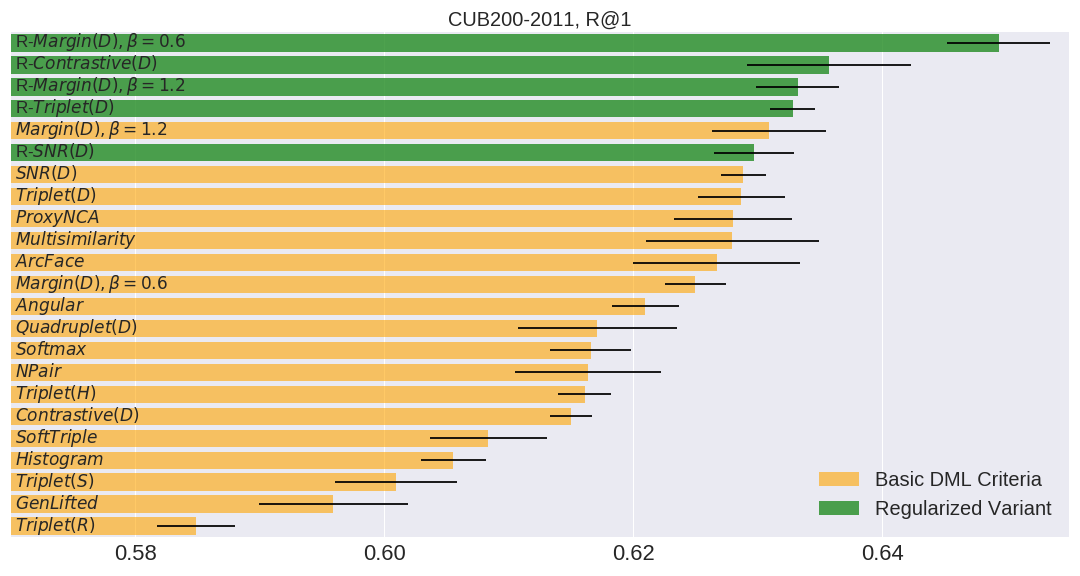
Figure 1: Mean recall performance and standard deviation of various DML objectives trained with (green) and without (orange) our proposed regularization. For all benchmarks, see appendix.

Learning visual similarity is important for a wide range of vision tasks, such as image clustering (Bouchacourt et al., 2018), face detection (Schroff et al., 2015) or image retrieval (Wu et al., 2017). Measuring similarity requires learning an embedding space which captures images and reasonably reflects similarities using a defined distance metric. One of the most adopted classes of algorithms for this task is Deep Metric Learning (DML) which leverages deep neural networks to learn such a distance preserving embedding.
Due to the growing interest in DML, a large corpus of literature has been proposed contributing to its success. However, as recent DML approaches explore more diverse research directions such as architectures (Xuan et al., 2018; Jacob et al., 2019), objectives functions (Wang et al., 2019b; Yuan et al., 2019) and additional training tasks (Roth et al., 2019; Lin et al., 2018), an unbiased comparison of their results becomes more and more difficult. Further, undisclosed technical details (s.a. data augmentations or training regularization) pose a challenge to the reproducibility of such methods, which is of great concern in the machine learning community in general (Bouthillier et al., 2019). One goal of this work is to counteract this worrying trend by providing a comprehensive comparison of important and current DML baselines under identical training conditions on standard benchmark datasets (Fig. 1). In addition, we thoroughly review common design choices of DML models which strongly influence generalization performance to allow for better comparability of current and future work.
On that basis, we extend our analysis to: (i) The process of data sampling which is well-known to impact the DML optimization (Schroff et al., 2015). While previous works only studied this process in the specific context of triplet mining strategies for ranking-based objectives (Wu et al., 2017; Harwood et al., 2017), we examine the model-agnostic case of sampling informative mini-batches. (ii) The generalization capabilities of DML models by analyzing the structure of their learned embedding spaces. While we are not able to reliably link typically targeted concepts such as large inter-class margins (Liu et al., 2017; Deng et al., 2018) and intra-class variance (Lin et al., 2018) to generalization performance, we uncover a strong correlation to the compression of the learned representations. Lastly, based on this observation, we propose a simple, yet effective, regularization technique which effectively boosts the performance of ranking-based approaches on standard benchmark datasets as also demonstrated in Fig. 1. In summary, our most important contributions can be described as follows:

• We provide an exhaustive analysis of recent DML objective functions, their training strategies, the influence of data-sampling, and model design choices to set a standard benchmark. To this end, we will make our code publicly available.

• We provide new insights into DML generalization by analyzing its correlation to the embedding space compression (as measured by its spectral decay), inter-class margins and intra-class variance.

• Based on the result above, we propose a simple technique to regularize the embedding space compression which we find to boost generalization performance of ranking-based DML approaches.

This work is structured as follows: After reviewing related work in §2, we discuss and motivate our analyzed components of DML models and their training setup in §3. Finally in §4 we present the findings of our study, analyze DML generalization in §5 and close with a conclusion in §6.

2 Related Works

Deep Metric Learning: Deep Metric Learning (DML) has become increasingly important for applications ranging from image retrieval (Movshovitz-Attias et al., 2017; Roth et al., 2019; Wu et al., 2017; Lin et al., 2018) to zero-shot classification (Schroff et al., 2015; Sanakoyeu et al., 2019) and face verification (Hu et al., 2014; Liu et al., 2017). Many approaches use ranking-based objectives based on tuples of samples such as pairs (Hadsell et al., 2006), triplets (Wu et al., 2017; Yu et al., 2018), quadruplets(Chen et al., 2017) or higher-order variants like N-Pairs(Sohn, 2016), lifted structure losses (Oh Song et al., 2016; Yu et al., 2018) or NCA-based criteria(Movshovitz-Attias et al., 2017). Further, classification-based methods adjusted to DML (Deng et al., 2018; Zhai & Wu, 2018) have proven to be effective for learning distance preserving embedding spaces. To address the computational complexity of tuple-based methods, different sampling strategies have been introduced (Schroff et al., 2015; Wu et al., 2017; Ge, 2018; Roth et al., 2020). Moreover, proxy-based approaches address this issue by approximating class distributions using only few virtual representatives (Movshovitz-Attias et al., 2017; Qian et al., 2019).
Additionally, more involved research extending above objectives has been proposed: Sanakoyeu et al. (2019) follow a divide-and-conquer strategy by splitting and subsequently merging both the data and embedding space; Opitz et al. (2018); Xuan et al. (2018) employ an ensemble of specialized learners and Roth et al. (2019); Milbich et al. (2020a, b) combine DML with feature mining or self-supervised learning. Moreover, Lin et al. (2018) and Zheng et al. (2019) generate artificial samples to effectively augment the training data, thus learning more complex ranking relations. The majority of these methods are trained using the essential objective functions and, further, hinge on the training parameters discussed in our study, thus directly benefiting from our findings. Moreover, we propose an effective regularization technique to improve ranking-based objectives.
Mini-batch selection: The benefits of large mini-batches for training are well studied (Smith et al., 2017; Goyal et al., 2017; Keskar et al., 2016). However, there has been limited research examining effective strategies for the creation of mini-batches. Research into mini-batch creation has been done to improve convergence in optimization methods for classification tasks(Mirzasoleiman et al., 2020; Johnson & Guestrin, 2018) or to construct informative mini-batches using core-set selection to optimize generative models (Sinha et al., 2019). Similarly, we analyze mining strategies maximizing data diversity and compare their impact to standard heuristics employed in DML (Wu et al., 2017; Roth et al., 2019; Sanakoyeu et al., 2019)).
Generalization in DML: Generalization capabilities of representations (Achille & Soatto, 2016; Shwartz-Ziv & Tishby, 2017) and, in particular, of discriminative models has been well studied (Jiang* et al., 2020; Belghazi et al., 2018; Goyal et al., 2017), e.g. in the light of compression (Tishby & Zaslavsky, 2015; Shwartz-Ziv & Tishby, 2017) which is covered by strong experimental support (Goyal et al., 2019; Belghazi et al., 2018; Alemi et al., 2016). Verma et al. (2018) link compression to a ’flattening’ of a representation in the context of classification. We apply this concept to analyze generalization in DML and find that strong compression actually hurts DML generalization. Existing works on generalization in metric learning focus on robustness of linear or kernel-based distance metrics (Bellet & Habrard, 2015; Bellet, 2013) and examine bounds on the generalization error (Huai et al., 2019). In contrast, we examine the correlation between generalization and structural characteristics of the learned embedding space.

3 Training a Deep Metric Learning Model

In this section, we briefly summarize key components for training a DML model and motivate the main aspects of our study. We first introduce the common categories of training objectives which we consider for comparison in Sec. 3.1. Next, in Sec. 3.2 we examine the data sampling process and present strategies for sampling informative mini-batches. Finally, in Sec. 3.3, we discuss components of a DML model which impact its performance and exhibit an increased divergence in the field, thus impairing objective comparisons.

3.1 The objective function

In Deep Metric Learning we learn an embedding function $\phi:\mathcal{X}\mapsto\Phi\subseteq\mathbb{R}^{D}$ mapping datapoints $x\in\mathcal{X}$ into an embedding space $\Phi$, which allows to measure the similarity between $x_{i},x_{j}$ as $d_{\phi}(x_{i},x_{j}):=d(\phi(x_{i}),\phi(x_{j}))$ with $d(.,.)$ being a predefined distance function. For that, let $\phi:=\phi_{\theta}$ be a deep neural network parametrised by $\theta$ with its output typically normalized to the real hypersphere $\mathbb{S}^{D}$ for regularization purposes (Wu et al., 2017; Huai et al., 2019). In order to train $\phi_{\theta}$ to reflect the semantic similarity defined by given labels $y\in\mathcal{Y}$, many objective functions have been proposed based on different concepts which we now briefly summarize.
Ranking-based: The most popular family are ranking-based loss functions operating on pairs (Hadsell et al., 2006), triplets (Schroff et al., 2015; Wu et al., 2017) or larger sets of datapoints (Sohn, 2016; Oh Song et al., 2016; Chen et al., 2017; Wang et al., 2019b). Learning $\phi_{\theta}$ is defined as an ordering task, such that the distances $d_{\phi}(x_{a},x_{p})$ between an anchor $x_{a}$ and positive $x_{p}$ of the same class, $y_{a}=y_{p}$, is minimized and the distances $d_{\phi}(x_{a},x_{n})$ of to negative samples $x_{n}$ with different class labels, $y_{a}\neq y_{n}$, is maximized. For example, triplet-based formulations typically optimize their relative distances as long as a margin $\gamma$ is violated, i.e. as long as $d_{\phi}(x_{a},x_{n})-d_{\phi}(x_{a},x_{p})<\gamma$. Further, ranking-based objectives are also extended to histogram matching, as proposed in (Ustinova & Lempitsky, 2016).
Classification-based: As DML is essentially solving a discriminative task, some approaches (Zhai & Wu, 2018; Deng et al., 2018; Liu et al., 2017) can be derived from softmax-logits $l_{i}=W_{j}^{T}\phi(x_{i})+b_{j}$. For example, Deng et al. (2018) exploit the regularization to the real hypersphere $\mathbb{S}^{D}$ and the equality $W_{j}^{T}x_{i}=\left\lVert W_{j}^{T}\right\rVert\left\lVert\phi(x_{i})\right\rVert\cos\varphi_{j}$ to maximize the margin between classes by direct optimization over angles $\varphi_{j}$. Further, also standard cross-entropy optimization proves to be effective under normalization (Zhai & Wu, 2018).
Proxy-based: These methods approximate the distributions for the full class by one (Movshovitz-Attias et al., 2017) or more (Qian et al., 2019) learned representatives. By considering the class representatives for computing the training loss, individual samples are directly compared to an entire class. Additionally, proxy-based methods help to alleviate the issue of tuple mining which is encountered in ranking-based loss functions.

3.2 Data sampling

The synergy between tuple mining strategies and ranking losses has been widely studied (Wu et al., 2017; Schroff et al., 2015; Ge, 2018). To analyze the impact of data-sampling on performance in the scope of our study, we consider the process of mining informative mini-batches $\mathcal{B}$. This process is independent of the specific training objective and so far has been commonly neglected in DML research. Following we present batch mining strategies operating on both labels and the data itself: label samplers, which are sampling heuristics that follow selection rules based on label information only, and embedded samplers, which operate on data embeddings themselves to create batches $\mathcal{B}$ of diverse data statistics.
Label Samplers: To control the class distribution within $\mathcal{B}$, we examine two different heuristics based on the number, $n$, of ’Samples Per Class’ (SPC-$n$) heuristic:
SPC-2/4/8: Given batch-size $b$, we randomly select $b/n$ unique classes from which we select $n$ samples randomly.
SPC-R: We randomly select $b-1$ samples from the dataset and choose the last sample to have the same label as one of the other $b-1$ samples to ensure that at least one triplet can be mined from $\mathcal{B}$. Thus, we effectively vary the number of unique classes within mini-batches.
Embedded Samplers: Increasing the batch-size $b$ has proven to be beneficial for stabilizing optimization due to an effectively larger data diversity and richer training information (Mirzasoleiman et al., 2020; Brock et al., 2018; Sinha et al., 2019). As the DML training is commonly performed on a single GPU (limited especially due to tuple mining process on the mini-batch), the batch-size $b$ is bounded by memory. Nevertheless, in order to ‘virtually’ maximize the data diversity, we distill the information content of a large set of samples $\mathcal{B}^{*},b^{*}=|\mathcal{B}^{*}|>b$ into a mini-batch $B$ by matching the statistics of $\mathcal{B}$ and $\mathcal{B}^{*}$ under the embedding $\phi$. To avoid computational overhead, we sample $\mathcal{B}^{*}$ from a continuously updated memory bank $\mathcal{M}$ of embedded training samples. Similar to Misra & van der Maaten (2019), $\mathcal{M}$ is generated by iteratively updating its elements based on the steady stream of training batches $\mathcal{B}$. Using $\mathcal{M}$, we mine mini-batches by first randomly sampling $\mathcal{B}^{*}$ from $\mathcal{M}$ with $b^{*}=1024$ and subsequently find a mini-batch $\mathcal{B}$ to match its data statistics by using one of the following criteria:
Greedy Coreset Distillation (GC): Greedy Coreset (Agarwal et al., 2005) finds a batch $\mathcal{B}$ by iteratively adding samples $x^{*}\in\mathcal{B}^{*}$ which maximize the distance from the samples that have already been selected $x\in\mathcal{B}$, thereby maximizing the covered space within $\Phi$ by solving $\min_{\mathcal{B}:|\mathcal{B}|=b}\max_{x*\in\mathcal{B}^{*}}\min_{x\in\mathcal{B}}d_{\phi}(x,x^{*})$.
Matching of distance distributions (DDM): DDM aims to preserve the distance distribution of $\mathcal{B}^{*}$. We randomly select $m$ candidate mini-batches and choose the batch $\mathcal{B}$ with smallest Wasserstein distance between normalized distance histograms of $\mathcal{B}$ and $\mathcal{B}^{*}$ (Rubner et al., 2000).
FRD-Score Matching (FRD): Similar to the recent GAN evaluation setting, we compute the frechet distance (Heusel et al., 2017)) between $\mathcal{B}$ and $\mathcal{B}^{*}$ to measure the similarity between their distributions using $FRD(\mathcal{B},\mathcal{B}^{*})=\left\|\mu_{\mathcal{B}}-\mu_{\mathcal{B}^{*}}\right\|_{2}^{2}+\text{Tr}(\Sigma_{\mathcal{B}}+\Sigma_{\mathcal{B}^{*}}-2(\Sigma_{\mathcal{B}}\Sigma_{\mathcal{B}^{*}})^{1/2})$, with $\mu_{\bullet},\Sigma_{\bullet}$ being the mean and covariance of the embedded set of samples. Like in DDM, we select the closest batch $\mathcal{B}$ to $\mathcal{B}^{*}$ among $m$ randomly sampled candidates.

3.3 Training parameters, regularization and architecture

Network	GN	IBN	R50
CUB200, R@1	45.41	48.78	43.77
CARS196, R@1	35.31	43.36	36.39
SOP, R@1	44.28	49.05	48.65

Table 1: Recall performance of commonly used network architectures after ImageNet pretraining. Final linear layer is randomly initialized and normalized.

Next to the objectives and data sampling process, successful learning hinges on a reasonable choice of the training environment. While there is a multitude of parameters to be set, we identify several factors which both influence performance and exhibit an divergence in lately proposed works.
Architectures: In recent DML literature predominantly three basis network architectures are used: GoogLeNet (Szegedy et al., 2015) (GN, typically with embedding dimensionality 512), Inception-BN (Ioffe & Szegedy, 2015) (IBN, 512) and ResNet50 (He et al., 2016) (R50, 128) (with optionally frozen Batch-Normalization layers for improved convergence and stability across varying batch sizes, see e.g. Roth et al. (2019); Cakir et al. (2019)). Due to the varying number of parameters and configuration of layers, each architecture exhibits a different starting point for learning, based on its initialization by ImageNet pretraining (Deng et al., 2009). Table 1 compares their initial DML performance measured in Recall@1 (R@1). The reference to differences in architecture is one of the main arguments used by individual works not compare themselves to competing approaches. Disconcertingly, even when reporting additional results using adjusted networks is feasible, typically only results using a single architecture are reported. Consequently, a fair comparison between approaches is heavily impaired.
Weight Decay: Commonly, network optimization is regularized using weight decay/L2-regularization (Krogh & Hertz, 1992). In DML, particularly on small datasets its careful adjustment is crucial to maximize generalization performance. Nevertheless, many works do not report this.
Embedding dimensionality: Choosing a dimensionality $D$ of the embedding space $\Phi$ influences the learned manifold and consequently generalization performance. While each architecture typically uses an individual, standardized dimensionality $D$ in DML, recent works differ without reporting proper baselines using an adjusted dimensionality. Again, comparison to existing works and the assessment of the actual contribution is impaired.
Data Preprocessing: Preprocessing training images typically significantly influences both the learned features and model regularization. Thus, as recent approaches vary in their applied augmentation protocols, results are not necessarily comparable. This includes the trend for increased training and test image sizes.
Batchsize: Batchsize determines the nature of the gradient updates to the network, e.g. datasets with many classes benefit from large batchsizes due to better approximations of the training distribution. However, it is commonly not taken into account as a influential factor of variation.
Advanced DML methodologies There are many extensions to objective functions, architectures and the training setup discussed so far. However, although extensions are highly individual, they still rely on these components and thus benefit from findings in the following experiments, evaluations and analysis.

4 Analyzing DML training strategies

Datasets

As benchmarking datasets, we use:
CUB200-2011: Contains 11,788 images in 200 classes of birds. Train/Test sets are made up of the first/last 100 classes (5,864/5,924 images respectively) (Wah et al., 2011). Samples are distributed evenly across classes.
CARS196: Has 16,185 images/196 car classes with even sample distribution. Train/Test sets use the first/last 98 classes (8054/8131 images) (Krause et al., 2013).
Stanford Online Products (SOP): Contains 120,053 product images divided into 22,634 classes. Train/Test sets are provided, contain 11,318 classes/59,551 images in the Train and 11,316 classes/60,502 images in the Test set (Oh Song et al., 2016). In SOP, unlike the other benchmarks, most classes have few instances, leading to significantly different data distribution compared to CUB200-2011 and CARS196.

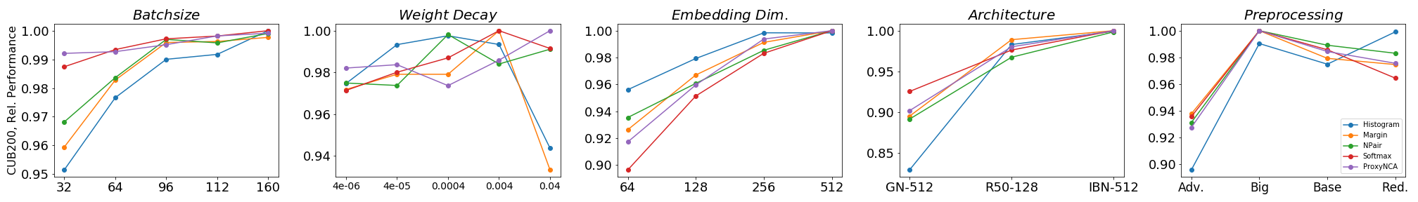
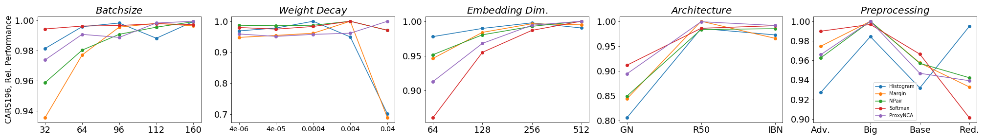
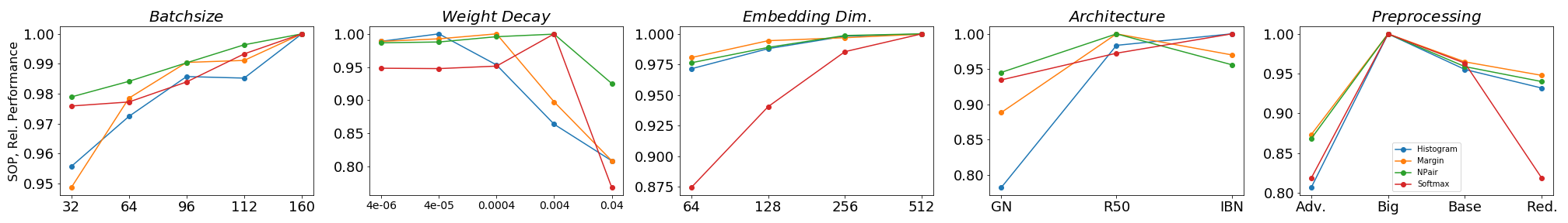
Figure 2: Evaluation of DML pipeline parameters and architectures on all benchmark datasets and their influence on relative improvement across different training criteria.

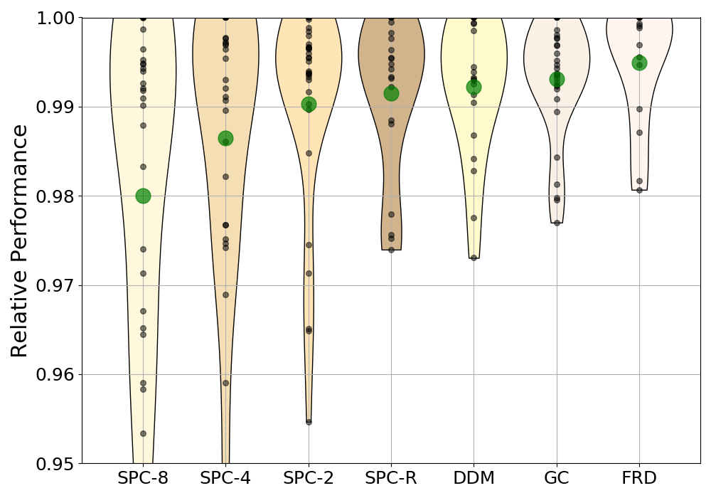
(a) CUB200-2011

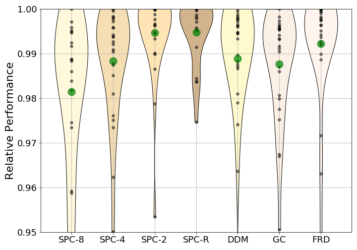
(b) CARS196

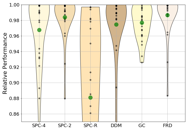
(c) SOP

Figure 3: Comparison of mini-batch mining strategies on three different datasets. Performance measures Recall@1 and 2, NMI, mAP and F1 are normalized across metrics and loss function. We plot the distributions of relative performances for each strategy.

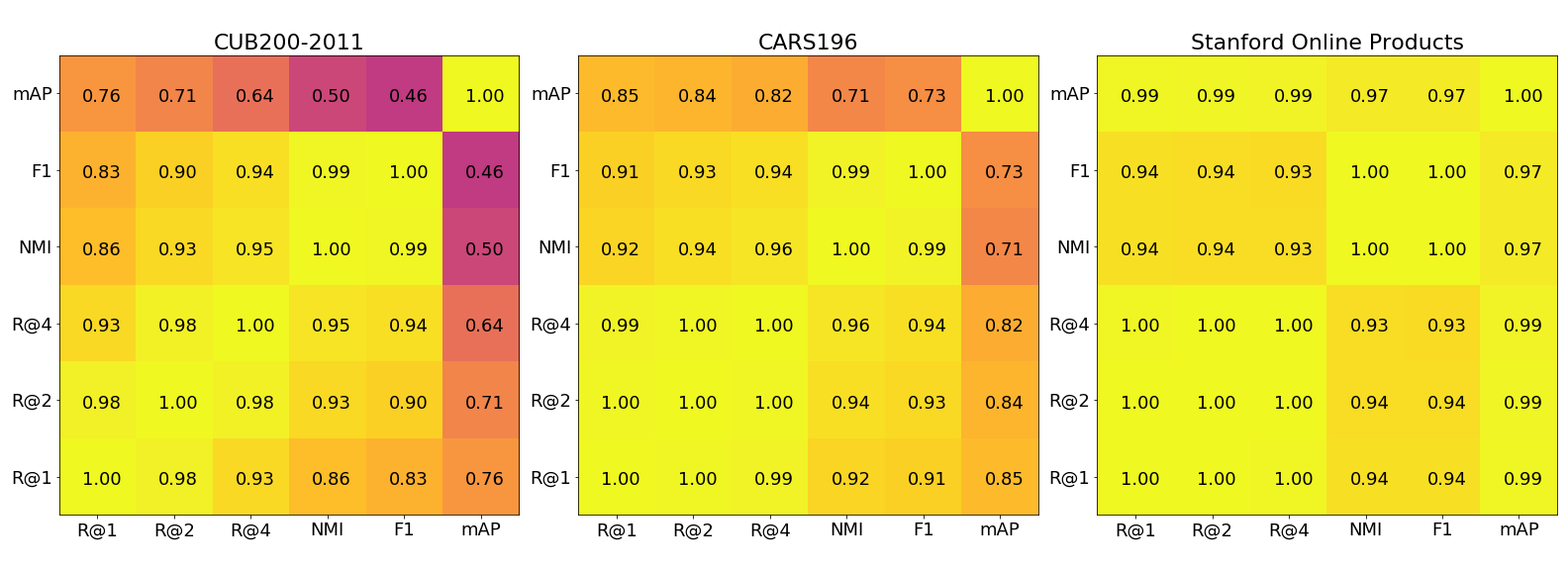
Figure 4: Metrics Correlation matrix for standard (Recall, NMI) and underreported retrieval metrics. mAP denotes mAP@C. Please refer to the supplementary for more information.

4.1 Experimental Protocol

Our training protocol follows parts of Wu et al. (2017), which utilize a ResNet50 architecture with frozen Batch-Normalization layers and embedding dim. 128 to be comparable with already proposed results with this architecture. While both GoogLeNet (Szegedy et al., 2015) and Inception-BN (Ioffe & Szegedy, 2015) are also often employed in DML literature, we choose ResNet50 due to its success in recent state-of-the-art approaches (Roth et al., 2019; Sanakoyeu et al., 2019). In line with standard practices we randomly resize and crop images to $224\times 224$ for training and center crop to the same size for evaluation. During training, random horizontal flipping ($p=0.5$) is used. Optimization is performed using Adam (Kingma & Ba, 2015) with learning rate fixed to $10^{-5}$ and no learning rate scheduling for unbiased comparison. Weight decay is set to a constant value of $4\cdot 10^{-4}$, as motivated in section 4.2. We implemented all models in PyTorch (Paszke et al., 2017), and experiments are performed on individual Nvidia Titan X, V100 and T4 GPUs with memory usage limited to 12GB. Each training is run over 150 epochs for CUB200-2011/CARS196 and 100 epochs for Stanford Online Products, if not stated otherwise. For batch sampling we utilize the the SPC-2 strategy, as motivated in section 4.3. Finally, each result is averaged over multiple seeds to avoid seed-based performance fluctuations. All loss-specific hyperparameters are discussed in the supplementary material, along with their original implementation details. For our study, we examine the following evaluation metrics (described further in the supplementary): Recall at 1 and 2 (Jegou et al., 2011), Normalized Mutual Information (NMI) (Manning et al., 2010), F1 score (Sohn, 2016), mean average precision measured on recall of the number of samples per class (mAP@C) and mean average precision measured on the recall of 1000 samples (mAP@1000). Please see the supplementary (supp. A.3) for more information.

4.2 Studying DML parameters and architectures

Benchmarks$\rightarrow$	CUB200-2011		CARS196		SOP
Approaches $\downarrow$	R@1	NMI	R@1	NMI	R@1	NMI
Imagenet (Deng et al., 2009)	$43.77$	$57.56$	$36.39$	$37.96$	$48.65$	$58.64$
Angular (Wang et al., 2017)	$62.10\pm 0.27$	$67.59\pm 0.26$	$78.00\pm 0.32$	$66.48\pm 0.44$	$73.22\pm 0.07$	$89.53\pm 0.01$
ArcFace (Deng et al., 2018)	$62.67\pm 0.67$	$67.66\pm 0.38$	$79.16\pm 0.97$	$66.99\pm 1.08$	$77.71\pm 0.15$	$90.09\pm 0.03$
Contrastive (Hadsell et al., 2006) (D)	$61.50\pm 0.17$	$66.45\pm 0.27$	$75.78\pm 0.39$	$64.04\pm 0.13$	$73.21\pm 0.04$	$89.78\pm 0.02$
GenLifted (Hermans et al., 2017)	$59.59\pm 0.60$	$65.63\pm 0.14$	$72.17\pm 0.38$	$63.75\pm 0.35$	$75.21\pm 0.12$	$89.84\pm 0.01$
Hist. (Ustinova & Lempitsky, 2016)	$60.55\pm 0.26$	$65.26\pm 0.23$	$76.47\pm 0.38$	$64.15\pm 0.36$	$71.30\pm 0.10$	$88.93\pm 0.02$
Margin (D, $\beta=0.6$) (Wu et al., 2017)	$62.50\pm 0.24$	$67.02\pm 0.37$	$77.70\pm 0.32$	$65.29\pm 0.32$	$77.38\pm 0.11$	$\mathbf{90.45\pm 0.03}$
Margin (D, $\beta=1.2$) (Wu et al., 2017)	$\mathbf{63.09\pm 0.46}$	$68.21\pm 0.33$	$79.86\pm 0.33$	$67.36\pm 0.34$	$\mathbf{78.43\pm 0.07}$	$90.40\pm 0.03$
Multisimilarity (Wang et al., 2019a)	$62.80\pm 0.70$	$\mathbf{68.55\pm 0.38}$	$\mathbf{81.68\pm 0.19}$	$\mathbf{69.43\pm 0.38}$	$77.99\pm 0.09$	$90.00\pm 0.02$
Npair (Sohn, 2016)	$61.63\pm 0.58$	$67.64\pm 0.37$	$77.48\pm 0.28$	$66.55\pm 0.19$	$75.86\pm 0.08$	$89.79\pm 0.03$
Pnca (Movshovitz-Attias et al., 2017)	$62.80\pm 0.48$	$66.93\pm 0.38$	$78.48\pm 0.58$	$65.76\pm 0.22$	$-$	$-$
Quadruplet (D) (Chen et al., 2017)	$61.71\pm 0.63$	$66.60\pm 0.41$	$76.34\pm 0.27$	$64.79\pm 0.50$	$76.95\pm 0.10$	$90.14\pm 0.02$
SNR (D) (Yuan et al., 2019)	$62.88\pm 0.18$	$67.16\pm 0.25$	$78.69\pm 0.19$	$65.84\pm 0.52$	$77.61\pm 0.34$	$90.10\pm 0.08$
SoftTriple (Qian et al., 2019)	$60.83\pm 0.47$	$64.27\pm 0.36$	$75.66\pm 0.46$	$62.66\pm 0.16$	$-$	$-$
Softmax (Zhai & Wu, 2018)	$61.66\pm 0.33$	$66.77\pm 0.36$	$78.91\pm 0.27$	$66.35\pm 0.30$	$76.92\pm 0.64$	$89.82\pm 0.15$
Triplet (D) (Wu et al., 2017)	$62.87\pm 0.35$	$67.53\pm 0.14$	$79.13\pm 0.27$	$65.90\pm 0.18$	$77.39\pm 0.15$	$90.06\pm 0.02$
Triplet (H) (Roth & Brattoli, 2019)	$61.61\pm 0.21$	$65.98\pm 0.41$	$77.60\pm 0.33$	$65.37\pm 0.26$	$73.50\pm 0.09$	$89.25\pm 0.03$
Triplet (R) (Schroff et al., 2015)	$58.48\pm 0.31$	$63.84\pm 0.30$	$70.63\pm 0.43$	$61.09\pm 0.27$	$67.86\pm 0.14$	$88.35\pm 0.04$
Triplet (S) (Schroff et al., 2015)	$60.09\pm 0.49$	$65.59\pm 0.29$	$72.51\pm 0.47$	$62.84\pm 0.41$	$73.61\pm 0.14$	$89.35\pm 0.02$
R-Contrastive (D)	$63.57\pm 0.66$	$67.63\pm 0.31$	$81.06\pm 0.41$	$67.27\pm 0.46$	$74.36\pm 0.11$	$89.94\pm 0.02$
R-Margin (D, $\beta=0.6$)	$\mathbf{64.93\pm 0.42}$	$68.36\pm 0.32$	$\mathbf{82.37\pm 0.13}$	$68.66\pm 0.47$	$77.58\pm 0.11$	$90.42\pm 0.03$
R-Margin (D, $\beta=1.2$)	$63.32\pm 0.33$	$67.91\pm 0.66$	$81.11\pm 0.49$	$67.72\pm 0.79$	$\mathbf{78.52\pm 0.10}$	$90.33\pm 0.02$
R-SNR (D)	$62.97\pm 0.32$	$68.04\pm 0.34$	$80.38\pm 0.35$	$67.60\pm 0.20$	$77.69\pm 0.25$	$90.02\pm 0.06$
R-Triplet (D)	$63.28\pm 0.18$	$67.86\pm 0.51$	$81.17\pm 0.11$	$67.79\pm 0.23$	$77.33\pm 0.14$	$89.98\pm 0.04$

Table 2: Comparison of Recall@1 and NMI performances for all objectives averaged over 5 runs. Each model is trained using the same training setting over 150 epochs for CUB/CARS and 100 epochs for SOP. ’R-’ denotes model trained with $\rho$-regularization. Bold denotes best results excluding regularization. Boldblue marks overall best results. Please note that a ranking on all other metrics (s.a. mAP@C, mAP@1000) as well as a visual summary can be found in the supplementary (supp. I, supp. C)!

Now we study the influence of parameters & architectures discussed in Sec. 3.3 using five different objectives. For each experiment, all metrics noted in Sec. 4.1 are measured. For each loss, every metric is normalized by the maximum across the evaluated value range. This enables an aggregated summary of performance across all metrics, where differences correspond to relative improvement. Fig. 2 analyzes each factor by evaluating a range of potential setups with the other parameters fixed to values from Sec. 4.1: Increasing the batchsize generally improves results with gains varying among criteria, with particularly high relevance on the SOP dataset. For weight decay, we observe loss and dataset dependent behavior up to a relative performance change of $5\%$. Varying the data preprocessing protocol, e.g. augmentations and input image size, leads to large performance differences as well. Base follows our protocol described in Sec. 4.1. Red. refers to resizing of the smallest image side to $256$ and cropping to $224$x$224$ with horizontal flipping. Big uses Base but crops images to $256$x$256$. Finally, we extend Base to Adv. with color jittering, changes in brightness and hue. We find that larger images provide better performance regardless of objective or dataset. Using the Adv. processing on the other hand is dependent on the dataset. Finally, we show that random resized cropping is a generally stronger operation than basic resizing and cropping.
All these factors underline the importance of a complete declaration of the training protocol to facilitate reproducibility and comparability. Similar results are observed for the choice of architecture and embedding dimensionality $D$. At the example of R50, our analysis shows that training objectives perform differently for a given $D$ but seem to converge at $D=512$. However, for R50 $D$ is typically fixed to $128$, thus disadvantaging some training objectives over others. Finally, comparing common DML architectures reveals their strong impact on performance with varying variance between loss functions. Highest consistencies seem to be achievable with R50 and IBN-based setups.
Implications: In order to warrant unbiased comparability, equal and transparent training protocols and model architectures are essential, as even small deviations can result in large deviations in performance.

4.3 Batch sampling impacts DML training

We now analyze how the data sampling process for mini-batches impacts the performance of DML models using the sampling strategies presented in Sec. 3.2. To conduct an unbiased study, we experiment with six conceptually different objective functions: Marginloss with Distance-Weighted Sampling, Triplet Loss with Random Sampling, ProxyNCA, Multi-Similarity Loss, Histogram loss and Normalized Softmax loss. To aggregate our evaluation metrics (cf. 4.1), we utilize the same normalization procedure discussed in Sec. 4.2. Fig. 3 summarizes the results for each sampling strategy by reporting the distributions of normalized scores of all pairwise combinations of training loss and evaluation metrics. Our analysis reveals that the batch sampling process indeed effects DML training with a difference in mean performance up to $1.5\%$. While there is no clear winner across all datasets, we observe that the SPC-2 and FRD samplers perform very well and, in particular, consistently outperform the SPC-4 strategy which is commonly reported to be used in literature (Wu et al., 2017; Schroff et al., 2015).
Implications: Our study indicates that DML benefits from data diversity in mini-batches, independent of the chosen training objective. This coincides with the general benefit of larger batchsizes as noted in section 4.2. While complex mining strategies may perform better, simple heuristics like SPC-2 are sufficient.

4.4 Comparing DML models

Based on our training parameter and batch-sampling evaluations we compare a large selection of $14$ different DML objectives and $4$ mining methods under fixed training conditions (see 4.1 & 4.2), most of which claim state-of-the-art by a notable margin. For ranking-based models, we employ distance-based tuple mining (D) (Wu et al., 2017) which proved most effective. We also include random, semihard sampling (Schroff et al., 2015) and a soft version of hard sampling (Roth & Brattoli, 2019) for our tuple mining study using the classic triplet loss. Loss-specific hyperparameters are determined via small cross-validation gridsearches around originally proposed values to adjust for our training setup. Exact parameters and method details are listed in supp. A.1. Table 2 summarizes our evaluation results on all benchmarks (with other metric rankings s.a. mAP@C or mAP@1000 in the supplementary (supp. I)), while Fig. 4 measures correlations between all evaluation metrics. Particularly on CUB200-2011 and CARS196 we find a higher performance saturation between methods as compared to SOP due to strong differences in data distribution. Generally, performance between criteria is much more similar than literature indicates, (see also concurrent work by Musgrave et al. (2020)). We find that representatives of ranking-based objectives outperform their classification/NCE-based counterparts, though not significantly. On average, margin loss (Wu et al., 2017) and multisimilarity loss (Wang et al., 2019a) offer the best performance across datasets, though not by a notable margin. Remarkably, under our carefully chosen training setting, a multitude of losses compete or even outperform more involved state-of-the-art DML approaches on the SOP dataset. For a detailed comparison to the state-of-the-art, we refer to the supplementary (supp. F).
Implications: Under the same setup, performance saturates across methods, contrasting results reported in literature. Taking into account standard deviations, usually left unreported, improvements become even less significant. In addition, carefully trained baseline models are able to outperform state-of-the-art approaches which use considerable stronger architectures. Thus, to evaluate the true benefit of proposed contributions, baseline models need to be competitive and implemented under comparable settings.

5 Generalization in Deep Metric Learning

The previous section showed how different model and training parameter choices result in vastly different performances. However, how such differences can be explained best on basis of the learned embedding space is an open question and, for instance, studied under the concept of compression (Tishby & Zaslavsky, 2015). Recent work (Verma et al., 2018) links compression to class-conditioned flattening of representation, indicated by an increased decay of singular values obtained by Singular Value Decomposition (SVD) on the data representations. Thus, class representations occupy a more compact volume, thereby reducing the number of directions with significant variance. The subsequent strong focus on the most discriminative directions is shown to be beneficial for classic classification scenarios with i.i.d. train and test distributions. However, this overly discards features which could capture data characteristics outside the training distribution. Hence, generalization in transfer problems like DML is hindered due to the shift in training and testing distribution (Bellet & Habrard, 2015). We thus hypothesize that actually retaining a considerable amount of directions of significant variance (DoV) is crucial to learn a well generalizing embedding function $\phi$.
To verify this assumption, we analyze the spectral decay of the embedded training data $\Phi_{\mathcal{X}}:=\{\phi(x)|x\in\mathcal{X}\}$ via SVD. We then normalize the sorted spectrum of singular values (SV) $\mathcal{S}_{\Phi_{\mathcal{X}}}$ and compute the KL-divergence to a D-dim. discrete uniform distribution $\mathcal{U}_{D}$, i.e. $\rho(\Phi)=\text{KL}(\mathcal{U}_{D}\;||\;\mathcal{S}_{\Phi_{\mathcal{X}}})$. We don’t consider individual training class representations, as testing and training distribution are shifted. Lower values of $\rho(\Phi)$ indicate more directions of significant variance. Using this measure, we analyze a large selection of DML objectives in Fig. 5 (rightmost) on CUB200-2011, CARS196 and SOP. Comparing R@1 and $\rho(\Phi)$ reveals significant inverse correlation ($\leq-0.63$) between generalization and the spectral decay of embedding spaces $\Phi$, which highlights the benefit of more directions of variance in the presence of train-test distribution shifts.
We now compare our finding to commonly exploited concepts for training such as (i) larger margins between classes (Deng et al., 2018; Liu et al., 2017), i.e. an increase in average inter-class distances $\pi_{\text{inter}}(\Phi)=\frac{1}{Z_{\text{inter}}}\sum_{y_{l},y_{k},l\neq k}d(\mu(\Phi_{y_{l}}),\mu(\Phi_{y_{k}}))$ ; (ii) explicitly introducing intra-class variance (Lin et al., 2018), which is indicated by an increase in average intra-class distance $\pi_{\text{intra}}(\Phi)=\frac{1}{Z_{\text{intra}}}\sum_{y_{l}\in\mathcal{Y}}\sum_{\phi_{i},\phi_{j}\in\Phi_{y_{l}},i\neq j}d(\phi_{i},\phi_{j})$. We also investigate (iii) their relation by using the ratio $\pi_{\text{ratio}}(\Phi)=\pi_{\text{intra}}(\Phi)/\pi_{\text{inter}}(\Phi)$, which can be regarded as an embedding space density. Here, $\Phi_{y_{l}}=\{\phi_{i}:=\phi_{\theta}(x_{i})|x_{i}\in\mathcal{X},y_{i}=y_{l}\}$ denotes the set of embedded samples of a class $y_{l}$, $\mu(\Phi_{y_{l}})$ their mean embedding and $Z_{\text{inter}},Z_{\text{intra}}$ normalization constants. Fig. 5 compares these measures with $\rho(\Phi)$. It is evident that neither of the distance related measures $\pi_{\bullet}(\Phi)$ consistently exhibits significant correlation with generalization performance when taking all three datasets into account. For CUB200-2011 and CARS196, we however find that an increased embedding space density ($\pi_{\text{ratio}})$ is linked to stronger generalisation. For SOP, its estimate is likely too noisy due to the strong imbalance between dataset size and amount of samples per class.
Implications: Generalization in DML exhibits strong inverse correlation to the SV spectrum decay of learned representations, as well as a weaker correlation to the embedding space density. This indicates that representation learning under considerable shifts between training and testing distribution is hurt by excessive feature compression, but may benefit from a more densely populated embedding space.

5.1 $\rho$-regularization for improved generalization

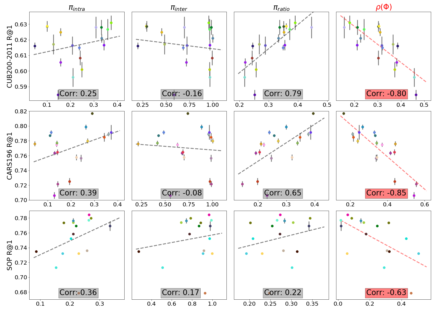
Figure 5: Correlation between generalization and structural properties derived from $\Phi_{\mathcal{X}}$ using different DML objectives on each dataset. Left-to-Right: Mean intra-class distances $\pi_{\text{intra}}$ & inter-class distances $\pi_{\text{inter}}$, the ratio $\pi_{\text{intra}}/\pi_{\text{inter}}$ and spectral decay $\rho$.

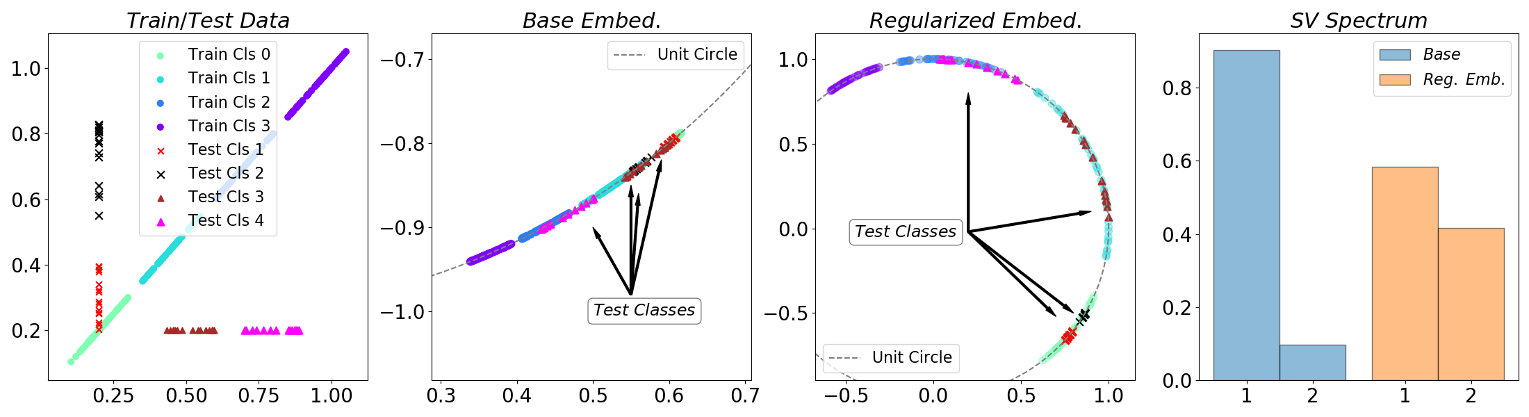
Figure 6: Toy example illustrating the effect of $\rho$-regularization. (Leftmost) training and test data. (Mid-left) A small, normalized two-layer fully-connected network trained with standard contrastive loss fails to separate all test classes due to excessive compression of the learned embedding. (Mid-right) The regularized embedding successfully separates the test classes by introducing a lower spectral decay. (Rightmost) Singular value spectra of training embeddings learned with and without regularization.

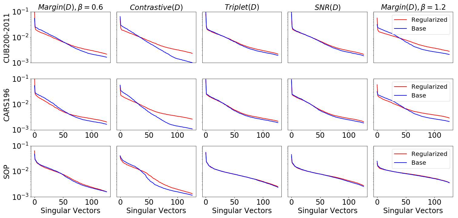
Figure 7: Sing. Value Spectrum for models trained with (red) and without (blue) $\rho$-regularization for various ranking-based criteria.

We now exploit our findings to propose a simple $\rho$-regularization for ranking-based approaches by counteracting the compression of representations. We randomly alter tuples by switching negative samples $x_{n}$ with the positive $x_{p}$ in a given ranking-loss formulation (cf. Sec. 3.1) with probability $p_{\text{switch}}$. This pushes samples of the same class apart, enabling a DML model to capture extra non-label-discriminative features while dampening the compression induced by strong discriminative training signals.
Fig. 6 depicts a 2D toy example (details supp. G) illustrating the effect of our proposed regularization while highlighting the issue of overly compressed data representations. Even though the training distribution exhibits features needed to separate all test classes, these features are disregarded by the strong discriminative training signal. Regularizing the compression by attenuating the spectral decay $\rho(\Phi)$ enables the model to capture more information and exhibit stronger generalization to the unseen test classes. In addition, Fig. 7 verifies that the $\rho$-regularization also leads to a decreased spectral decay on DML benchmark datasets, resulting in improved recall performance (cf. Tab. 2 (bottom)), while being reasonably robust to changes in $p_{\text{switch}}$ (see supp. B). In contrast, in the appendix we also see that encouraging higher compression seems to be detrimental to performance.
Implications: Implicitly regularizing the number of directions of significant variance can improve generalization.

6 Conclusion

In this work, we counteract the worrying trend of diverging training protocols in Deep Metric Learning (DML). We conduct a large, comprehensive study of important training components and objectives in DML to contribute to improved comparability of recent and future approaches. On this basis, we study generalization in DML and uncover a strong correlation to the level of compression and embedding density of learned data representation. Our findings reveal that highly compressed representations disregard helpful features for capturing data characteristics that transfer to unknown test distributions. To this end, we propose a simple technique for ranking-based methods to regularize the compression of the learned embedding space, which results in boosted performance across all benchmark datasets.

Reviewer Comments

Re: Data Augmentation/Different Spatial Resolution: We agree that data augmentation is an important factor to regularize training. We have made sure to analyze the impact of different image augmentations and resolutions on the performance.

Re: In-Shop dataset experiments: The data distribution of the In-Shop dataset is very similar to the SOP dataset, thus relative results are generally transferable, which is why we have decided not to include it in this work.

Re: Grammar and typos: We thank the reviewers for pointing out these errors and have made sure to correct them.

Re: Missing references: All mentioned references have been added.

Appendix A Description of Methods

In this section, we briefly describe each DML training objective and triplet mining strategy used in our study, as well as the choice of their individual hyperparameters. General training parameters and details of the training protocol are already discussed in the main paper in Sec. 4.1. For notation, we refer to the embedding of an image $x_{i}$ including output normalization as $\phi_{i}=\phi(x_{i})$. The non-normalized version is denoted as $\phi^{*}_{i}$. All methods operate on the mini-batch $\mathcal{B}$ containing image indices. If not mentioned otherwise, all embeddings operate in dimension $D=128$.

A.1 Training Criteria

Contrastive (Hadsell et al., 2006)

The contrastive training formalism is simple: Given embedding pairs $\mathcal{P}$ (sampled from a mini-batch of size $b$) containing an anchor $\phi_{a}$ from class $y_{a}$ and either a positive $\phi_{p}$ with $y_{p}=y_{a}$ or a negative $\phi_{n}$ from a different class, $y_{n}\neq y_{a}$, the network $\phi$ is trained to minimize

$$\mathcal{L}_{contr}=\frac{1}{b}\sum^{b}_{(i,j)\in\mathcal{P}}\mathbb{I}_{y_{i}=y_{j}}d_{e}(\phi_{i},\phi_{j})+\mathbb{I}_{y_{i}\neq y_{j}}[\gamma-d_{e}(\phi_{i},\phi_{j})]_{+}$$ (1)

with margin $\gamma$, which we set to $1$. The margin ensures that embeddings are not projected arbitrarily far apart from each other. For our distance function we utilize the standard euclidean distance $d_{e}(x,y)=\left\|x-y\right\|_{2}$. We combine the contrastive loss with the distance-weighting negative sampling mentioned below.

Triplet (Hu et al., 2014)

Triplets extend the contrastive formalism to provide a concurrent ranking surrogate for both negative and positive sample embeddings using triplets $\mathcal{T}$ sampled from a mini-batch:

$$\mathcal{L}_{tripl}=\frac{1}{b}\sum^{b}_{\begin{subarray}{c}(a,p,n)\in\mathcal{T}\\ y_{a}=y_{p}\neq y_{n}\end{subarray}}\left[d_{e}(\phi_{a},\phi_{p})-d_{e}(\phi_{a},\phi_{n})+\gamma\right]_{+}$$ (2)

with margin $\gamma=0.2$, thus following recent implementations in e.g. Roth et al. (2019) or (Wu et al., 2017). Initial works (Schroff et al., 2015) using the triplet loss commonly utilized random or semihard triplet sampling and a GoogLeNet-based architecture. Recent methods typically employ the more effective distance-weighted sampling (Wu et al., 2017) and more powerful networks (Roth et al., 2019; Sanakoyeu et al., 2019). For completeness, we compare the triplet-loss performance combinde with random, semihard and distance-weighted sampling schemes introduced below.

Generalized Lifted Structure (Hermans et al., 2017)

The Generalized Lifted Structure loss extends the standard lifted structure loss (Oh Song et al., 2016) to include all available anchor-positive and anchor-negative distance pairs within a mini-batch $\mathcal{B}$, instead of utilizing only a single anchor-positive combination:

$$\mathcal{L}_{genlift}=\sum_{a\in\mathcal{B}}\left[\log\sum_{p\in\mathcal{B},y_{a}=y_{p}}\exp{\left(d_{e}(\phi^{*}_{a},\phi^{*}_{p})\right)}+\log\sum_{n\in\mathcal{B},y_{n}\neq y_{a}}\exp{\left(\gamma-d_{e}(\phi^{*}_{a},\phi^{*}_{n})\right)}\right]_{+}+\frac{\nu}{b}\cdot\sum_{a\in\mathcal{B}}\left\|\phi^{*}_{a}\right\|_{2}^{2}$$ (3)

with mini-batch samples of a class $c$ grouped into $C$, and sets of $C$ contained in $\mathcal{C}$. $\phi^{*}$ denotes the non-normalized version of $\phi$. The margin $\gamma=1$ serves the standard purpose of avoiding over-distancing already correct image pairs. To account for increasing values, $\nu=0.005$ regularizes the embeddings.

N-Pair (Sohn, 2016)

N-Pair or N-Tuple losses extend the triplet formalism to incorporate all negatives in the mini-batch $\mathcal{B}$ by

$$\mathcal{L}_{npair}=\frac{1}{b}\sum_{\begin{subarray}{c}(a,p)\in\mathcal{B}\\ y_{a}=y_{p},a\neq p\end{subarray}}\log\left(1+\sum_{\begin{subarray}{c}n\in\mathcal{B}\\ y_{a}\neq y_{n}\end{subarray}}\exp{(\phi_{a}^{*,T}\phi_{n}-\phi_{a}^{*,T}\phi^{*}_{p})}\right)+\frac{\nu}{b}\cdot\sum_{i\in\mathcal{B}}\left\|\phi^{*}_{i}\right\|_{2}^{2}$$ (4)

with embedding regularization $\nu=0.005$, as (Sohn, 2016) noted a slow convergence for normalized embeddings.

Angular (Wang et al., 2017)

By introducing an angle-based penalty, the angular loss effectively introduces scale invariance and higher-order geometric constraints that are not explicitly introduced in normal contrastive losses:

$$\mathcal{L}_{ang}=\mathcal{L}_{npair}(\phi^{*})+\frac{\lambda}{b}\sum_{\begin{subarray}{c}(a,p)\in\mathcal{B}\\ y_{a}=y_{p},a\neq p\end{subarray}}\left[\log(1+\sum_{\begin{subarray}{c}n\in\mathcal{B}\\ y_{n}\neq y_{a}\end{subarray}}\exp{\left(4\tan^{2}\left(\alpha(\phi_{a}+\phi_{p})^{T}\phi_{n}\right)\right)-2\left(1+\tan^{2}(\alpha)\right)\phi_{a}^{T}\phi_{n}}\right]$$ (5)

with angular margin $\alpha$, which, as proposed in the original paper, is set to $\pi/4$. $\lambda=2$ is the trade-off between standard ranking losses and the angular constraint. The N-Pair parameters are set as above.

Arcface (Deng et al., 2018)

Arcface transforms the standard softmax formulation typically used in classification problem to retrieval-based problems by enforcing an angular margin between the embeddings $\phi$ and an approximate center $W\in\mathbb{R}^{c\times d}$ for each class, resulting in

$$\mathcal{L}_{arc}=-\frac{1}{b}\sum_{i\in\mathcal{B}}\log\frac{\exp(s\cdot\cos{(W_{y_{i}}^{T}\phi_{i}+\gamma=0.5)})}{\exp{(s\cdot\cos{(W_{y_{i}}^{T}\phi_{i}+\gamma=0.5)})}+\sum_{\begin{subarray}{c}j\in\mathcal{B}\\ y_{i}\neq y_{j}\end{subarray}}\exp{(s\cdot\cos{(W_{y_{j}}^{T}\phi_{i})})}}$$ (6)

Further, this training objective also introduces the additive angular margin penalty $\gamma=0.5$ for increased inter-class discrepancy, while the scaling $s=16$ denotes the radius of the effective utilized hypersphere $\mathbb{S}$. The class centers are optimized with learning rate $0.0005$.

Histogram (Ustinova & Lempitsky, 2016)

In contrast to many sample-based ranking objective functions, Histogram Loss learns to minimize the probability of a positive sample pair having a higher similarity score than a negative pair. Given a mini-batch $\mathcal{B}$, the sets of positive similarities $\mathcal{S}^{+}=\{\phi_{i}^{T}\phi_{j}|(i,j)\in\mathcal{P},y_{i}=y_{j}\}$ and negative similarities $\mathcal{S}^{-}=\{\phi_{i}^{T}\phi_{j}|(i,j)\in\mathcal{P},y_{i}\neq y_{j}\}$, one optimises

$$\delta(s,r) =\frac{1}{\Delta}\left(\mathbb{I}_{s\in[t_{r-1},t_{r}]}\cdot(s-t_{r-1})+\mathbb{I}_{s\in[t_{r-1},t_{r}]}\cdot(t_{r+1}-s)\right)$$ (7)

$$h^{+/-}(r) =\frac{1}{\|\mathcal{S}^{+/-}\|}\sum_{s\in\mathcal{S}^{+/-}}\delta(s,r)$$ (8)

$$\mathcal{L}_{hist} =\sum_{r\in R}h^{-}(r)\left(\sum_{q=1}^{r}h^{+}(q)\right)$$ (9)

resulting in soft, differentiable histogram assignments. The final objective $\mathcal{L}_{hist}$ then penalizes strong overlap between the probability of positive pairs having higher distance (i.e. its cumulative distribution to point $r$) than respective negative pairs. Such a histogram loss introduces a single hyperparameter, namely the degree of histogram discretisation $R$, which we set to $65$ for CUB200-2011 and CARS196 and $11$ for SOP in our study. In general, our implementation borrows from the original code base used in (Ustinova & Lempitsky, 2016).

Margin (Wu et al., 2017)

Margin loss extends the standard triplet loss by introducing a dynamic, learnable boundary $\beta$ between positive and negative pairs. This transfers the common triplet ranking problem to a relative ordering of pairs $\mathcal{P}=\{(i,j)|i,j\in\mathcal{B},y_{i}\neq y_{j}\}$:

$$\mathcal{L}_{margin}=\sum_{(i,j)\in\mathcal{P}}\gamma+\mathbb{I}_{y_{i}=y_{j}}(d(\phi_{i},\phi_{j})-\beta)-\mathbb{I}_{y_{i}\neq y_{j}}(d_{e}(\phi_{i},\phi_{j})-\beta)$$ (10)

The learning rate of the boundary $\beta$ is set to $0.0005$, with initial value either $0.6$ or $1.2$ and triplet margin $\gamma=0.2$. For our implementation, we utilise the distance-weighted triplet sampling method highlighted below.

MultiSimilarity (Wang et al., 2019a)

Unlike contrastive and triplet based ranking methods, the MultiSimilarity loss concurrently evaluates similarities between anchor and negative, anchor and positive, as well as positive-positive and negative-negative pairs in relation to an anchor:

$$s^{*}_{c}(i,j) =\begin{cases}s_{c}(\phi_{i},\phi_{j})\qquad s_{c}(\phi_{i},\phi_{j})>\min_{j\in\mathcal{P}_{i}}s_{c}(\phi_{i},\phi_{j})-\epsilon\\ s_{c}(\phi_{i},\phi_{j})\qquad s_{c}(\phi_{i},\phi_{j})<\max_{k\in\mathcal{N}_{i}}s_{c}(\phi_{i},\phi_{k})+\epsilon\\ 0\qquad\qquad\qquad\text{otherwise}\end{cases}$$ (11)

$$\mathcal{L}_{multisim} =\frac{1}{b}\sum_{i\in\mathcal{B}}\left[\frac{1}{\alpha}\log[1+\sum_{j\in\mathcal{P}_{i}}\exp(-\alpha(s^{*}_{c}(\phi_{i},\phi_{j})-\lambda))]+\frac{1}{\beta}\log[1+\sum_{k\in\mathcal{N}_{i}}\exp(\beta(s^{*}_{c}(\phi_{i},\phi_{k})-\lambda))]\right]$$ (12)

where $\mathcal{P}_{x}$ and $\mathcal{N}_{x}$ denote the set of positive and negative samples for a sample $x$, with cosine similarity $s_{c}(x,y)=x^{T}y$ for two normalized vectors $x,y\in\mathbb{R}^{d}$. For our hyperparameters, we use $\alpha=2$, $\beta=40$, $\lambda=0.5$ and $\epsilon=0.1$.

ProxyNCA (Movshovitz-Attias et al., 2017)

The sampling complexity of tuples heavily affects the training convergence. ProxyNCA introduces a remedy by introducing class proxies, which act as approximations to entire classes. This way only an anchor is sampled and compared against the respective positive and negative class proxies. Utilizing one proxy $\psi_{c}\in\mathbb{R}^{d}$ per class $c\in\mathcal{C}$, ProxyNCA is then defined as

$$\mathcal{L}_{proxy}=-\frac{1}{b}\sum_{i\in\mathcal{B}}\log\left(\frac{\exp(-d_{e}(\phi_{i},\psi_{y_{i}})}{\sum_{c\in\mathcal{C}\setminus\{y_{i}\}}\exp(-d(\phi_{i},\psi_{c})}\right)$$ (13)

Quadruplet (Chen et al., 2017)

The quadruplet loss is an extension to the triplet loss, which introduces higher level ordering constraint on sample embeddings. By using an anchor, a positive and two exclusive negatives, the quadruplet criterion is defined as:

$$\mathcal{L}_{Quadr}=\sum_{\begin{subarray}{c}i,j,k\in\mathcal{B}\\ y_{i}=y_{j},y_{j}\neq y_{k}\end{subarray}}\left[d(\phi_{i},\phi_{j})-d(\phi_{i},\phi_{k})+\gamma_{1}\right]_{+}+\sum_{\begin{subarray}{c}i,j,k,l\in\mathcal{B}\\ y_{i}=y_{j},y_{j}\neq y_{k},y_{l}\neq y_{k},y_{l}\neq y_{j}\end{subarray}}\left[d(\phi_{i},\phi_{k})-d(\phi_{l},\phi_{k})+\gamma_{2}\right]_{+}$$ (14)

with margin parameters $\gamma_{1}=1$ and $\gamma_{2}=0.5$. We utilize distance-weighted sampling to propose the first negative sample $k$, which we found to work better than the quadruplet sampling scheme originally proposed in the paper.

SNR (Yuan et al., 2019)

The Signal-to-Noise-Ratio loss (SNR) introduces a novel distance metric based on the ratio between anchor embedding variance and variance of noise, which is simply defined as the difference between anchor and compared embedding. This optimises the embedding space directly for informativeness. The complete loss can then be written as

$$\mathcal{L}_{SNR}=\sum_{i,j,k\in\mathcal{T}}\left[\frac{\sum_{m=1}^{D}(\phi_{i,m}-\phi_{j,m})}{\sum_{m=1}^{D}\phi_{i,m}^{2}}-\frac{\sum_{m=1}^{D}(\phi_{i,m}-\phi_{k,m})}{\sum_{m=1}^{D}\phi_{i,m}^{2}}+\gamma\right]_{+}+\frac{\lambda}{b}\sum_{i\in\mathcal{B}}\left\|\sum_{m=1}^{D}\phi_{i,m}\right\|$$ (15)

with margin parameter $\gamma=0.2$ and regularization $\lambda=0.005$ to ensure zero-mean distributions. Note that $\phi_{i,m}=\phi(x_{i})_{m}$.

SoftTriple (Qian et al., 2019)

Similar to ProxyNCA, the SoftTriple objective function utilizes learnable data proxies to tackle the sampling problem. However, instead of class-discriminative proxies, a set of normalized intra-class proxies $\psi\in\Psi^{c}$ per class $c$ are learned using the NCA-based similarity measure $\mathcal{S}_{i}^{c}$ of a sample $i$ to all proxies of a class $c$. Denoting the set of available classes as $\mathcal{C}$ and the total set of proxies as $\Psi$, we get

$$\mathcal{S}_{i}^{c} =\sum_{\psi\in\Psi^{c}}\frac{\exp(\frac{1}{\gamma}\phi_{i}^{T}\psi)}{\sum_{\psi\in\Psi^{c}}\exp(\frac{1}{\gamma}\phi_{i}^{T}\psi)}$$ (16)

$$\mathcal{L}_{STBase} =-\frac{1}{b}\sum_{i\in\mathcal{B}}\log\frac{\exp(\lambda(\mathcal{S}_{i}^{y_{i}}-\delta))}{\exp(\lambda(\mathcal{S}_{i}^{y_{i}}-\delta))+\sum_{y\in\mathcal{Y}\setminus\{y_{i}\}}\exp(\lambda\mathcal{S}_{i}^{y})}$$ (17)

$$\mathcal{L}_{SoftTriple} =\mathcal{L}_{STBase}+\tau\cdot\frac{\sum_{c\in\mathcal{C}}\sum_{\psi_{1},\psi_{2}\in\Psi^{c},\psi_{1}\neq\psi_{2}}\sqrt{2-2\psi_{1}^{T}\psi_{2}}}{|\mathcal{C}|\cdot|\Psi|\cdot(|\Psi|-1)}$$ (18)

The second term denotes a regularization on the learned proxies to ensure sparseness in the class set of proxies. For our tests, we utilised the following hyperparameter values (borrowing from the official implementation in (Qian et al., 2019)): $\tau=0.2$, $\lambda=8$, $\delta=0.01$, $\gamma=0.1$ and the number of proxies per class $|\Psi^{c}|=2$ (higher values resulted in much worse performance). The proxy learning rate is set to $0.00001$.

Normalized Softmax (Zhai & Wu, 2018)

Similar to other classification-based losses in DML that are based on re-formulations of the standard softmax function (such as $\mathcal{L}_{arc}$), the normalized softmax loss is optimized by comparing input embeddings $\phi_{i}$ to class proxies $\psi\in\mathbb{R}^{D}$ per class $c\in\mathcal{C}$:

$$\mathcal{L}_{NormSoft}=-\sum_{i\in\mathcal{B}}\log\left(\frac{\exp(\frac{\phi_{i}^{T}\psi_{y_{i}}}{T})}{\sum_{c\in\mathcal{C}\setminus\{y_{i}\}}\exp(\frac{\phi_{i}^{T}\psi_{c}}{T})}\right)$$ (19)

with temperature $T=0.05$ for gradient boosting and class proxy learning rate set to $10^{-5}$.

A.2 Tuple Mining

Basic contrastive, triplet or higher order ranking losses commonly need to mine their training tuples from the available mini-batch. In our study, we measure the influence of tuple sampling on the standard triplet loss, while utilising Distance-Weighted Mining for all ranking-based objective functions except N-Pair based methods.

Random Tuple Mining (Hu et al., 2014)

The trivial way involves the random sampling of tuples. Simply put, per sample $\{x_{i}\}_{i\in\mathcal{B}}$ we select a respective positive $\{j|y_{j}=y_{i},i\neq j,j\in\mathcal{B}\}$ or negative sample $\{k|y_{j}\neq y_{i},i\neq k,k\in\mathcal{B}\}$.

Semihard Triplet Mining (Schroff et al., 2015)

The potential number of triplets scales cubic in training set size. During learning, more and more of those triplets are correctly ordered and effectively provide no training signal (Schroff et al., 2015), thus impairing the remaining training process. To alleviate this, negative samples are carefully selected based on the anchor-positive sample distance (which are sampled at random). Given an anchor embedding $\phi_{a}$ and its positive $\phi_{p}$, the negative is sampled randomly from the set

$$\phi_{n}\in\{\phi_{n}|n\in\mathcal{B},y_{n}\neq y_{a},\left\|\phi_{a}-\phi_{p}\right\|_{2}^{2}<\left\|\phi_{a}-\phi_{n}\right\|_{2}^{2}\}.$$ (20)

This way, only negatives are considered which are reasonably hard to separate from an anchor. Moreover, this mining strategy avoids the sampling of overlay hard negatives, which often correspond to data noise and potentially lead to model collapses and bad local minima (Schroff et al., 2015).

Softhard Triplet Mining (Roth & Brattoli, 2019)

While it was justifiably noted in (Schroff et al., 2015) that a selection of ’hard’ samples hurts training, (Roth & Brattoli, 2019) show that a probabilistic (soft) selection of potentially hard candidates can actually benefit performance. Given an anchor embedding $\phi_{a}$, positive $\phi_{p}$ and $\phi_{n}$ are randomly selected from

$$\phi_{n}\in\{\phi_{n}|n\in\mathcal{B},y_{n}\neq y_{a},\left\|\phi_{a}-\phi_{n}\right\|_{2}^{2}<\operatorname*{arg\,max}_{p\in\mathcal{B},y_{a}=y_{p}}\left\|\phi_{a}-\phi_{p}\right\|_{2}^{2}\}$$ (21)

and

$$\phi_{a}\in\{\phi_{a}|a\in\mathcal{B},y_{n}=y_{a},\left\|\phi_{a}-\phi_{n}\right\|_{2}^{2}>\operatorname*{arg\,min}_{n\in\mathcal{B},y_{a}\neq y_{p}}\left\|\phi_{a}-\phi_{n}\right\|_{2}^{2}\}.$$ (22)

Doing so provides a selection of ’hard’ positivies and negatives. This reduces the risk of potential model collapses and bad local minima (as noted in Schroff et al. (2015)).

Distance-Weighted Tuple Mining (Wu et al., 2017)

In DML, the embedding spaces are typically normalized to a $D$-dimensional (unit) hypersphere $\mathbb{S}^{D-1}$ for regularisation purposes (Wu et al., 2017). The analytical distribution of pairwise distances on a hypersphere follows

$$q(d_{e}(\phi_{i},\phi_{j}))\propto d_{e}(\phi_{i},\phi_{j})^{D-2}[1-\frac{1}{4}d_{e}(\phi_{i},\phi_{j})]^{\frac{D-3}{2}}$$ (23)

for arbitrary embedding pairs $\phi_{i},\phi_{j}\in\mathbb{S}^{D-1}$. In order to sample negatives from the whole range of possible distances to an anchor, Wu et al. (2017) propose to sample negatives based on a distance distribution inverse to $q$, i.e.

$$P(n|a)\propto\min(\lambda,q^{-1}(d_{e}(\phi_{a},\phi_{n}))$$ (24)

We set $\lambda=0.5$ and limit the distances to $1.4$.

A.3 Evaluation Metrics

In this section, we examine the evaluation metrics to measure the performance of the studied models on a the testset $\mathcal{X_{\text{test}}}$.

Recall@k (Jegou et al., 2011)

Let

$$\mathcal{F}_{q}^{k}=\operatorname*{arg\,min}_{\mathcal{F}\subset\mathcal{X_{\text{test}}},|\mathcal{F}|=k}\sum_{x_{f}\in\mathcal{F}}d_{e}(\phi(x_{q}),\phi(x_{f}))$$ (25)

be the set of the first $k$ nearest neighbours of a sample $x_{p}$, then we measure Recall@k as

$$R@k=\frac{1}{|\mathcal{X_{\text{test}}}|}\sum_{x_{q}\in\mathcal{X_{\text{test}}}}\begin{cases}1\qquad\exists\;x_{i}\in\mathcal{F}_{q}^{k}\;\text{s.t.}\;y_{i}=y_{q}\\ 0\qquad\text{otherwise}\end{cases}$$ (26)

which measures the average number of cases in which for a given query $x_{q}$ there is at least one sample among its top $k$ nearest neighbours $x_{i}$ with the same class, i.e. $y_{i}=y_{q}$.

Normalized Mutual Information (NMI) (Manning et al., 2010)

To measure the clustering quality using NMI, we embed all samples $x_{i}\in\mathcal{X_{\text{test}}}$ to obtain $\Phi_{\mathcal{X_{\text{test}}}}$ and perform a clustering (e.g. $K$-Means (Lloyd, 1982)). Following, we assign all samples $x_{i}$ a cluster label $w_{i}$ indicating the closest cluster center and define $\Omega=\{\omega_{k}\}_{k=1}^{K}$ with $\omega_{k}=\{i|w_{i}=k\}$ and $K=|\mathcal{C}|$ being the number of classes and clusters. Similarly for the true labels $y_{i}$ we define $\Upsilon=\{\upsilon_{c}\}_{c=1}^{K}$ with $\upsilon_{c}=\{i|y_{i}=c\}$. The normalized mutual information is then computed as

$$NMI(\Omega,\Upsilon)=\frac{I(\Omega,\Upsilon)}{2(H(\Omega)+H(\Upsilon)}$$ (27)

with mutual Information $I(\cdot,\cdot)$ between cluster and labels, and entropy $H(\cdot,\cdot)$ on the clusters and labels respectively.

F1-Score (Sohn, 2016)

The F1-score measures the harmonic mean between precision and recall and is a commonly used retrieval metric, placing equal importance to both precision and recall. It is defined as

$$F1=\frac{2PR}{P+R}$$ (28)

with precision $P$ and Recall $R$ defined over nearest neighbour retrieval as done for Recall@k.

Mean Average Precision measured on Recall (mAP) @C and @1000:

The mAP-score measured on recall follows the same definition as standard mAP, however the recalled samples are determined by the nearest neighbour ranking. In our case, we propose to use mAP@C and mAP@C. mAP@C is equivalent to the mean over the class-wise average precision@$k_{c}$ with $k_{c}$ being the number of samples with label $c\in\mathcal{C}$, which only recalls as many samples as there are members in a class. For completeness, we also use mAP@1000, which recalls the 1000 nearest samples. With $\mathcal{F}^{k_{c}}_{q}$ defined as in eq. 25, this gives

$$\text{mAP@C}=\frac{1}{|\mathcal{X}_{\text{test}}|}\sum_{c\in\mathcal{C}}\sum_{x_{q}\in\mathcal{X}_{\text{test}}\wedge y_{q}=c}\frac{\left|\{x_{i}\in\mathcal{F}^{k_{c}}_{q}|y_{i}=y_{q}\}\right|}{k_{c}}$$ (29)

$$\text{mAP@1000}=\frac{1}{|\mathcal{X}_{\text{test}}|}\sum_{c\in\mathcal{C}}\sum_{x_{q}\in\mathcal{X}_{\text{test}}\wedge y_{q}=c}\frac{\left|\{x_{i}\in\mathcal{F}^{1000}_{q}|y_{i}=y_{q}\}\right|}{1000}$$ (30)

Appendix B Evaluating the robustness of $p_{\text{switch}}$ choices

For all benchmarks, we evaluate the change in performance for varying values of $p_{\text{switch}}$. As can be seen in figure 8, performance steadily increases up to a point of saturation, where the regulatory signal overshadows the discriminative one. In addition, its clear that performance increases are reasonably robust against changes in $p_{\text{switch}}$.

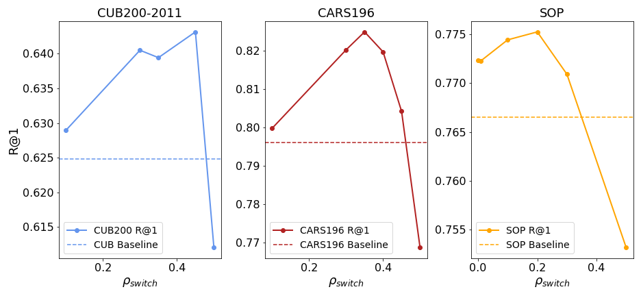
Figure 8: Analysis of the influence of $p_{\text{switch}}$ on Recall@1 using margin loss with $\beta=0.6$. Dashed lines denote performance without $\rho$-regularization.

Appendix C Visual comparison of DML objectives on benchmarks

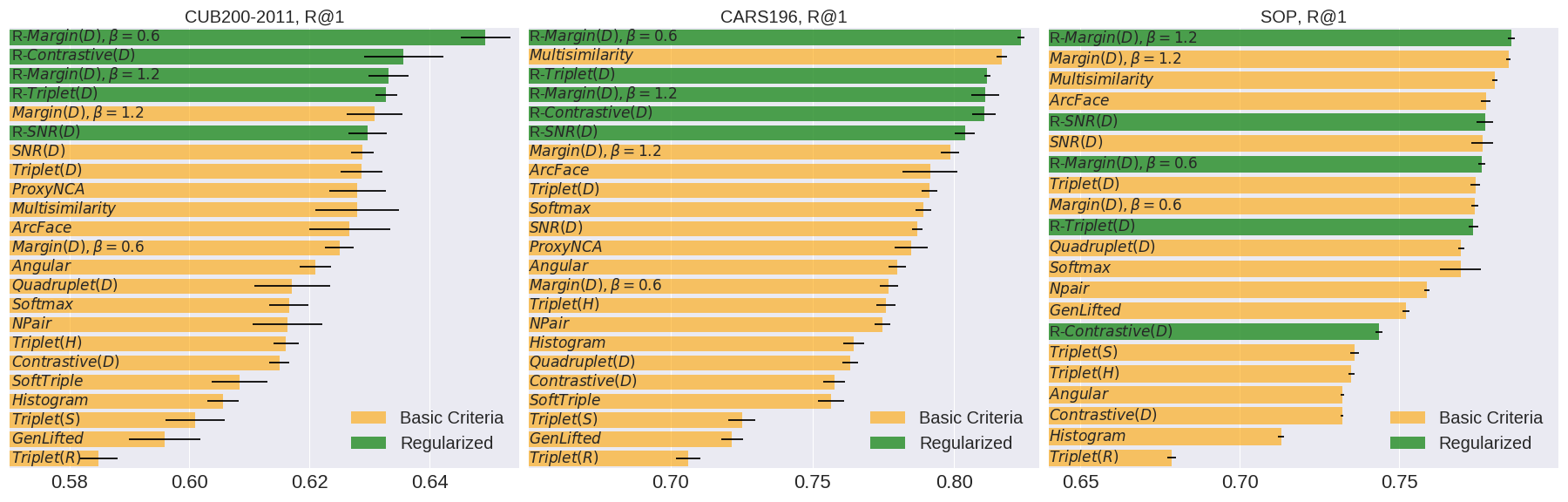
Figure 9: Mean recall performance and standard deviation of various DML objective functions trained with (green) and without (orange) our proposed regularization.

This figure is the full version of the first page figure (Fig. 1). It qualitatively supports the saturation of performance noted in section 4 and table 2.

Appendix D Correlation between performance and spectral decay $\rho$

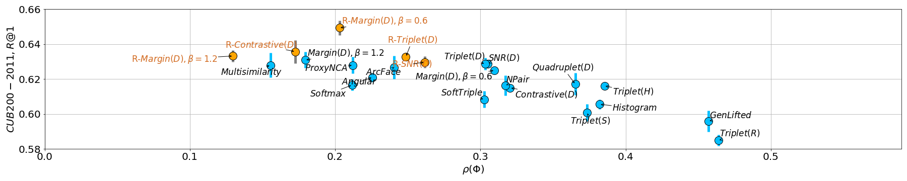
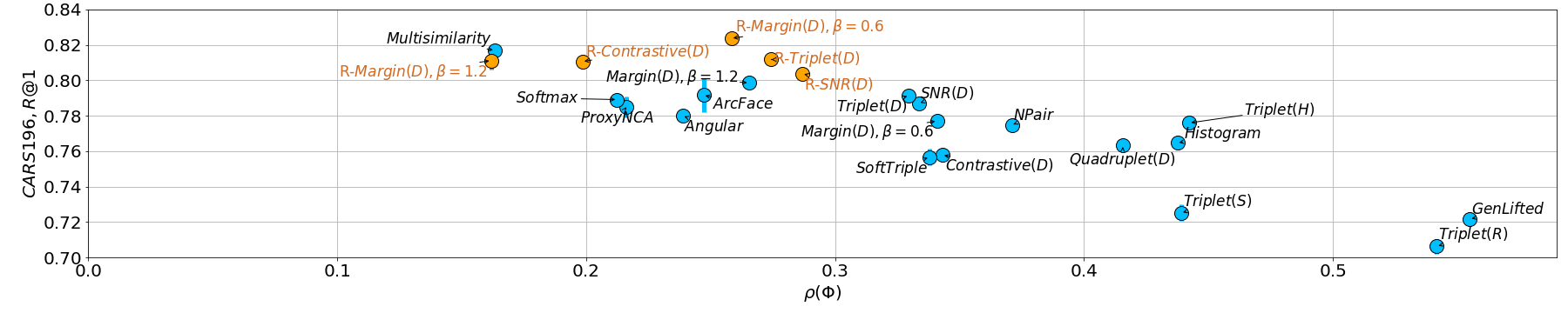
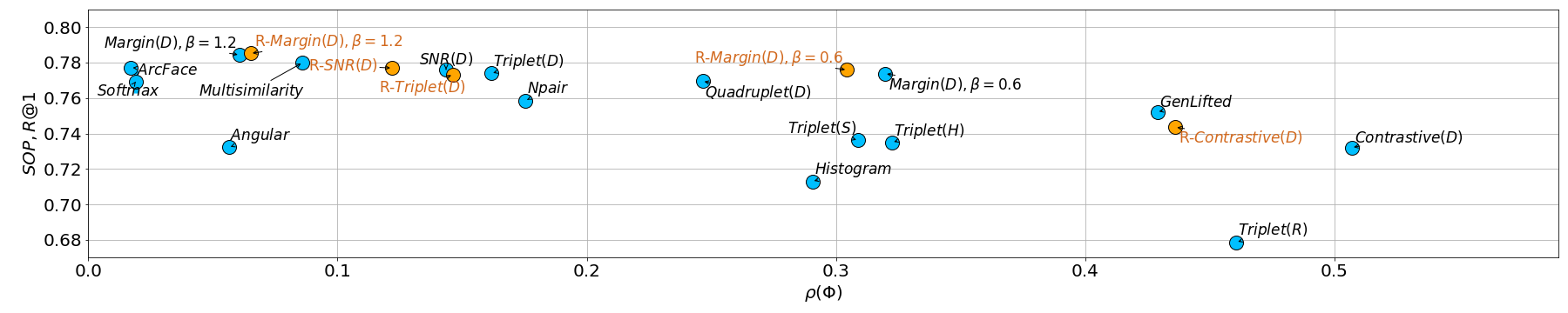
Figure 10: Relation between $\rho(\Phi)$ and generalization performance on Recall@1 for models trained with (orange) and without (blue) $\rho$-regularization. We report mean results and error-bars (gray). When error is small, bars are covered.

Similar to Fig. 5 (rightmost) in the main paper, we now provide a more detailed illustration in Fig. 10 comparing the performance of the training objectives and their corresponding spectral decay $\rho(\Phi)$. For ranking losses, we further include the results using $\rho$-regularization while training, which further shows that in each case a gain in performance is related to a decrease of $\rho(\Phi)$. Especially the contrastive loss (Hadsell et al., 2006) greatly profits from our proposed regularization, as also indicated by the analysis of the singular value spectra (cf. Fig. 8 of main paper). Its large gains, more then $5\%$ on the CARS196 dataset, is well explained by comparison of its training objective with those of triplet-based formulations. The latter optimizes over relative positive ($d_{\phi}(x_{a},x_{p})$)) and negative distances ($d_{\phi}(x_{a},x_{n})$) up to a fixed margin $\gamma$, which counteracts a compression of the embedding space to a certain extend. On the other hand, the constrastive loss, while controlling only the negative distances by $\gamma$, is able to perform an unconstrained contraction of entire classes, which facilitates overly compressed embedding spaces $\Phi$.

Appendix E Analysis of per-class singular value spectra

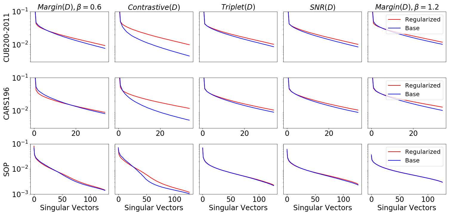
Figure 11: Averaged class-conditioned spectra of singular values for models trained with (red) and without (blue) $\rho$-regularization for various ranking-based loss functions.

In Sec. 5 of our main paper we analyze generalization in DML by considering the decay of the singular value spectrum over all embedded samples $\Phi_{\mathcal{X}}$. Thus, we analyze the general compression of the entire embedding space $\Phi$ as unseen test classes can be projected anywhere in $\Phi$, in contrast to Verma et al. (2018) which conduct a class-conditioned analysis for i.i.d. classification problems. In order to show that the effect of $\rho$-regularization (as shown in Fig. 8 in main paper) is also reflected in the class-conditioned singular value spectrum, we perform SVD on $\Phi_{y_{l}}$ and subsequently average over all classes $y_{l}\in\mathcal{Y}$. Fig. 11 compares the sorted, first $35$ singular values for both, models trained with and without $\rho$-regularization. We clearly see that the regularization decreases the average decay of singular values similar to the total singular value spectra shown in the main paper.

Appendix F Comparison to state-of-the-art approaches on SOP dataset

Approach	Architecture	Dim	R@1	R@10	R@100	NMI
DVML(Lin et al., 2018)	GoogLeNet	512	70.2	85.2	93.8	90.8
HTL(Ge, 2018)	Inception-BN	512	74.8	88.3	94.8	-
MIC(Roth et al., 2019)	ResNet50	128	77.2	89.4	95.6	90.0
D&C(Sanakoyeu et al., 2019)	ResNet50	128	75.9	88.4	94.9	90.2
Rank(Wang et al., 2019b)	Inception-BN	1536	79.8	91.3	96.3	90.4
ABE(Kim et al., 2018)	GoogLeNet	512	76.3	88.4	94.8	-
Margin (ours)(Wu et al., 2017)	ResNet50	128	78.4	-	-	90.4

Table 3: Comparison to the state-of-the-art DML methods on SOP(Oh Song et al., 2016). Dim denotes the dimensionality of $\phi_{\theta}$.

In this section we provide a detailed comparison between current state-of-the-art DML approaches and our strongest baseline model, margin loss (D, $\beta=1.2$) (Wu et al., 2017), on the SOP dataset in Tab. 6. The results for these approaches are taken from their public manuscripts. We observe that our baseline model outperforms each of the models using varying architectures, but especially other ResNet50-based implementations. While R50 proves to be a stronger base network (cf. Fig. 2 of main paper) than GoogLeNet based model, improvements over MIC and D&C using the same backbone by at least $0.9\%$ and methods based on the similarly strong Inception-BN showcase the relevance of a well-defined baseline. Additionally, even though Rank and ABE employ considerable more powerful network ensembles, our carefully motivated baseline exhibits competitive performance.

Appendix G 2D Toy Examples

For our toy examples, we use a fully-connected network with two 30 neuron layers. Both input and embedding dimension are 2D, while the latter is normalized onto the unit circle. Each of the four training and test lines contain 15 samples taken from either the diagonal or vertical/horizontal line segments, respectively. We train the networks both with and without regularization for $200$ iterations, a batchsize of $24$ and learning rate of $0.03$ using a standard contrastive loss (eq. 1) with margin $\gamma=0.1$. For regularisation, we set $p_{\text{switch}}=0.001$. Similar to Fig.6 in the main paper, Fig. 12 shows another 2D toy example based on vertical lines which again demonstrates the effect of compression and of our proposed $\rho$-regularization. The example consists of four training lines that are separable only by their $x$-coordinate and a test set of lines which are separable by their $y$-coordinate. As we observe, the test samples are collapsed onto a single point in the non-regularized embedding space, thus can not be distinguished. In contrast, the regularized representation allows us to separate the test classes and, further, exhibits a decreased decay in the singular value spectrum.

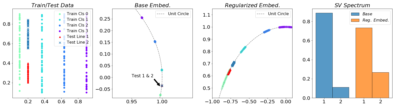
Figure 12: Toy example based on horizontally discriminative training data, where to goal is to generalize to vertically discriminative test data. (Leftmost) training and test data. (Mid-left) A small, normalized two-layer fully-connected network trained with standard contrastive loss fails to separate both test classes as it never has to utilize vertical discrimination. (Mid-right) The regularized embedding successfully separates the test classes by introducing additional features and decreasing the spectral decay. (Rightmost) Singular value spectra of training embeddings learned with and without regularization.

Appendix H Influence of Manifold Mixup on DML

Now, we examine the effect of applying the regularization proposed in ManifoldMixup (Verma et al., 2018) on the DML transfer learning setting. As ManifoldMixup has been proposed to increase the compression of a learned representation in the context of standard supervised classification, it is expected to decrease the performance of DML models. For that, we train three different DML models on the CUB200-2011 dataset: (1) Normalized Softmax, (2) Triplet with Distance Sampling and (3) Margin loss with $\beta=0.6$ and Distance Sampling. For (1), the implementation directly follows the standard implementation noted in Verma et al. (2018). For the ranking-based training objectives, we perform mixup in our ResNet50 and generate the mixed class labels, which consequently have either one (if image from the same class are mixed) or two entries (if images from different classes are mixed). Per (mixed) anchor embedding, this gives rise to up to two possible sets of triplets, for which we compute the loss and weigh it by the respective mixup coefficient $\lambda_{k}$:

$$\mathcal{L}_{tripl}^{\text{Mix}}=\frac{1}{b}\sum_{k=1}^{2}\sum^{b}_{\begin{subarray}{c}(a,p,n)\in\mathcal{T}^{k}\\ y_{a}=y_{p}\neq y_{n}\end{subarray}}\lambda_{k}\cdot\left[d_{e}(\phi^{\lambda}_{a},\phi^{\lambda}_{p})-d_{e}(\phi^{\lambda}_{a},\phi^{\lambda}_{n})+\gamma\right]_{+}$$ (31)

where $\mathcal{T}^{k}$ denotes the set of triplets given the $k$-th mixup class-label entry and $\lambda_{k}$ the respective interpolation value. We use the notation $\phi^{\lambda}_{x}$ to denote that we now operate on mixup embeddings. For training, we use the standard hyperparameters as described in Sec. 4.1. of the main paper and a mixup-$\alpha$ of $2$ to sample the interpolation values $\lambda\sim\beta(\alpha,\alpha)$ (see Verma et al. (2018)).
The results after rerunning baselines and mixup-variants are shown in Fig. 13. As expected, applying ManifoldMixup leads to more compressed representations (indicated by a stronger spectral decay and lower $\rho(\Phi)$-scores) at the cost of reduced generalization performance. This holds both for the spectrum across the fully embedded dataset as well as on a class level.

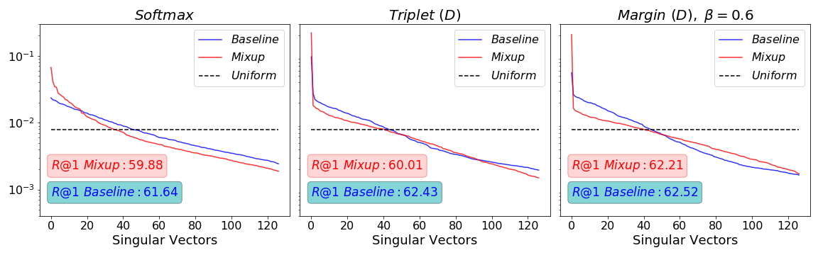
(a) Singular Value Spectrum for all embeddings

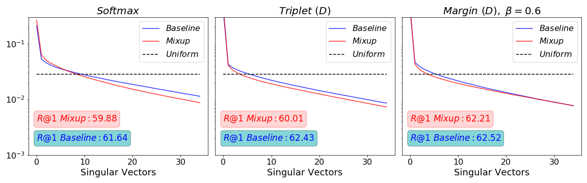
(b) Singular Value Spectrum for per-class embeddings

Figure 13: Evaluation of Mixup Influence on zero-shot generalization under heavy distribution shift.

Appendix I Detailed Results

This section contains detailed results per method and evaluation metric for the method comparisons (Tab. 2 in the main paper) and evaluation of batch-creation methods (Fig. 3 in main paper). The resp. tables for the method comparisons are Tab. 4 for CUB200-2011 (Wah et al., 2011), Tab. 5 for CARS196 (Krause et al., 2013) and Tab. 6 for Stanford Online Products (SOP) (Oh Song et al., 2016). In addition, the switch probability $p_{\text{switch}}$ for each regularised method is noted as well. The batch-creation methods are evaluated in detail in Tab. 7 for CUB200-2011, Tab. 8 for CARS196 and Tab. 9 for SOP.

CUB200-2011(Wah et al., 2011)
Approach	R@1	R@2	F1	mAP@C	mAP@1000	NMI
Imagenet	$43.77$	$57.56$	$19.14$	$9.48$	$14.62$	$52.91$
Angular	$62.10\pm 0.27$	$73.68\pm 0.39$	$37.53\pm 0.13$	$22.06\pm 0.20$	$30.56\pm 0.27$	$67.59\pm 0.26$
ArcFace	$62.67\pm 0.67$	$74.38\pm 0.25$	$37.33\pm 0.51$	$23.05\pm 0.43$	$31.62\pm 0.68$	$67.66\pm 0.38$
Contrastive (D)	$61.50\pm 0.17$	$72.95\pm 0.32$	$35.40\pm 0.75$	$23.46\pm 0.18$	$32.38\pm 0.21$	$66.45\pm 0.27$
GenLifted	$59.59\pm 0.60$	$71.63\pm 0.38$	$34.86\pm 0.16$	$22.03\pm 0.14$	$30.30\pm 0.13$	$65.63\pm 0.14$
Histogram	$60.55\pm 0.26$	$72.08\pm 0.20$	$33.88\pm 0.56$	$22.65\pm 0.20$	$31.24\pm 0.27$	$65.26\pm 0.23$
Multisimilarity	$62.80\pm 0.70$	$74.37\pm 0.52$	$39.03\pm 0.63$	$22.58\pm 0.37$	$30.92\pm 0.49$	$\mathbf{68.55\pm 0.38}$
Margin (D, $\beta=0.6$)	$62.50\pm 0.24$	$74.15\pm 0.33$	$36.34\pm 0.61$	$23.83\pm 0.20$	$32.90\pm 0.29$	$67.02\pm 0.37$
Margin (D, $\beta=1.2$)	$63.09\pm 0.46$	$74.41\pm 0.37$	$38.36\pm 0.66$	$23.61\pm 0.31$	$32.63\pm 0.40$	$68.21\pm 0.33$
NPair	$61.63\pm 0.58$	$73.33\pm 0.42$	$37.29\pm 0.42$	$22.16\pm 0.29$	$30.83\pm 0.30$	$67.64\pm 0.37$
ProxyNCA	$62.80\pm 0.48$	$74.03\pm 0.15$	$36.20\pm 0.73$	$23.94\pm 0.37$	$33.13\pm 0.59$	$66.93\pm 0.38$
Quadruplet (D)	$61.71\pm 0.63$	$73.26\pm 0.33$	$35.74\pm 0.62$	$23.20\pm 0.24$	$31.87\pm 0.29$	$66.60\pm 0.41$
SNR (D)	$62.88\pm 0.18$	$74.33\pm 0.26$	$36.91\pm 0.42$	$23.48\pm 0.14$	$32.24\pm 0.21$	$67.16\pm 0.25$
SoftTriple	$60.83\pm 0.47$	$71.61\pm 0.58$	$32.16\pm 0.50$	$22.43\pm 0.29$	$31.33\pm 0.29$	$64.27\pm 0.36$
Softmax	$61.66\pm 0.33$	$73.31\pm 0.39$	$35.94\pm 0.59$	$22.19\pm 0.20$	$30.67\pm 0.26$	$66.77\pm 0.36$
Triplet (D)	$62.87\pm 0.35$	$74.31\pm 0.28$	$37.30\pm 0.32$	$23.59\pm 0.12$	$32.64\pm 0.13$	$67.53\pm 0.14$
Triplet (R)	$58.48\pm 0.31$	$70.51\pm 0.24$	$31.95\pm 0.44$	$21.12\pm 0.10$	$29.08\pm 0.12$	$63.84\pm 0.30$
Triplet (S)	$60.09\pm 0.49$	$71.75\pm 0.27$	$34.46\pm 0.54$	$22.49\pm 0.26$	$31.40\pm 0.39$	$65.59\pm 0.29$
Triplet (H)	$61.61\pm 0.21$	$72.94\pm 0.34$	$35.10\pm 0.37$	$22.63\pm 0.23$	$31.22\pm 0.27$	$65.98\pm 0.41$
R-Contrastive (D)	$63.57\pm 0.66$	$74.57\pm 0.63$	$37.70\pm 0.53$	$23.54\pm 0.37$	$32.40\pm 0.66$	$67.63\pm 0.31$
R-Margin (D, $\beta=0.6$)	$\mathbf{64.93\pm 0.42}$	$\mathbf{75.58\pm 0.25}$	$\mathbf{38.93\pm 0.54}$	$\mathbf{24.11\pm 0.20}$	$\mathbf{33.38\pm 0.27}$	$68.36\pm 0.32$
R-Margin (D, $\beta=1.2$)	$63.32\pm 0.33$	$74.80\pm 0.27$	$38.09\pm 0.97$	$22.80\pm 0.46$	$31.44\pm 0.67$	$67.91\pm 0.66$
R-SNR (D)	$62.97\pm 0.32$	$74.66\pm 0.06$	$38.25\pm 0.41$	$23.13\pm 0.23$	$32.23\pm 0.47$	$68.04\pm 0.34$
R-Triplet (D)	$63.28\pm 0.18$	$74.97\pm 0.28$	$38.03\pm 0.77$	$23.28\pm 0.28$	$32.36\pm 0.47$	$67.86\pm 0.51$

Table 4: Comparison of DML setups for CUB200-2011. We report all relevant performance metrics. Training is done over 150 epochs.

CARS196(Krause et al., 2013)
Approach	R@1	R@2	F1	mAP@C	mAP@1000	NMI
Imagenet	$36.39$	$48.11$	$8.90$	$4.03$	$6.92$	$37.96$
Angular	$78.00\pm 0.32$	$85.97\pm 0.18$	$36.40\pm 0.75$	$22.18\pm 0.35$	$29.29\pm 0.37$	$66.48\pm 0.44$
ArcFace	$79.16\pm 0.97$	$87.02\pm 0.54$	$36.36\pm 1.97$	$23.44\pm 0.68$	$31.36\pm 0.99$	$66.99\pm 1.08$
Contrastive (D)	$75.78\pm 0.39$	$84.17\pm 0.27$	$33.10\pm 0.63$	$23.19\pm 0.33$	$30.43\pm 0.51$	$64.04\pm 0.13$
GenLifted	$72.17\pm 0.38$	$81.94\pm 0.30$	$32.46\pm 0.43$	$21.66\pm 0.24$	$28.66\pm 0.31$	$63.75\pm 0.35$
Histogram	$76.47\pm 0.38$	$84.50\pm 0.36$	$33.04\pm 0.67$	$23.21\pm 0.10$	$30.31\pm 0.14$	$64.15\pm 0.36$
Multisimilarity	$81.68\pm 0.19$	$88.86\pm 0.14$	$40.95\pm 0.72$	$24.22\pm 0.27$	$31.92\pm 0.44$	$\mathbf{69.43\pm 0.38}$
Margin (D, $\beta=0.6$)	$77.70\pm 0.32$	$85.67\pm 0.19$	$35.04\pm 0.49$	$24.08\pm 0.27$	$31.99\pm 0.29$	$65.29\pm 0.32$
Margin (D, $\beta=1.2$)	$79.86\pm 0.33$	$87.46\pm 0.20$	$38.44\pm 0.64$	$24.72\pm 0.21$	$32.50\pm 0.28$	$67.36\pm 0.34$
NPair	$77.48\pm 0.28$	$85.73\pm 0.18$	$35.88\pm 0.40$	$23.15\pm 0.25$	$30.70\pm 0.14$	$66.55\pm 0.19$
ProxyNCA	$78.48\pm 0.58$	$86.20\pm 0.50$	$34.66\pm 0.48$	$23.82\pm 0.36$	$31.86\pm 0.34$	$65.76\pm 0.22$
Quadruplet (D)	$76.34\pm 0.27$	$84.67\pm 0.23$	$34.28\pm 0.88$	$23.49\pm 0.32$	$31.30\pm 0.48$	$64.79\pm 0.50$
SNR (D)	$78.69\pm 0.19$	$86.44\pm 0.22$	$35.88\pm 0.71$	$24.20\pm 0.43$	$32.17\pm 0.60$	$65.84\pm 0.52$
SoftTriple	$75.66\pm 0.46$	$83.72\pm 0.29$	$31.07\pm 0.56$	$22.90\pm 0.25$	$30.42\pm 0.31$	$62.66\pm 0.16$
Softmax	$78.91\pm 0.27$	$86.66\pm 0.23$	$35.51\pm 0.85$	$22.81\pm 0.14$	$29.84\pm 0.13$	$66.35\pm 0.30$
Triplet (D)	$79.13\pm 0.27$	$86.74\pm 0.17$	$35.89\pm 0.25$	$24.38\pm 0.18$	$32.26\pm 0.25$	$65.90\pm 0.18$
Triplet (R)	$70.63\pm 0.43$	$80.43\pm 0.26$	$29.02\pm 0.47$	$19.48\pm 0.20$	$25.97\pm 0.28$	$61.09\pm 0.27$
Triplet (S)	$72.51\pm 0.47$	$81.53\pm 0.29$	$31.61\pm 0.41$	$21.63\pm 0.26$	$28.32\pm 0.56$	$62.84\pm 0.41$
Triplet (H)	$77.60\pm 0.33$	$85.63\pm 0.27$	$34.71\pm 0.31$	$23.84\pm 0.13$	$31.31\pm 0.15$	$65.37\pm 0.26$
R-Contrastive (D)	$81.06\pm 0.41$	$88.06\pm 0.21$	$37.72\pm 0.84$	$24.55\pm 0.34$	$32.53\pm 0.43$	$67.27\pm 0.46$
R-Margin (D, $\beta=0.6$)	$\mathbf{82.37\pm 0.13}$	$\mathbf{89.14\pm 0.12}$	$\mathbf{39.28\pm 0.41}$	$\mathbf{25.67\pm 0.32}$	$\mathbf{34.57\pm 0.30}$	$68.66\pm 0.47$
R-Margin (D, $\beta=1.2$)	$81.11\pm 0.49$	$88.20\pm 0.22$	$38.76\pm 0.94$	$24.17\pm 0.50$	$31.60\pm 0.79$	$67.72\pm 0.79$
R-SNR (D)	$80.38\pm 0.35$	$87.95\pm 0.37$	$38.62\pm 0.47$	$24.72\pm 0.15$	$33.02\pm 0.23$	$67.60\pm 0.20$
R-Triplet (D)	$81.17\pm 0.11$	$88.43\pm 0.18$	$38.72\pm 0.31$	$25.27\pm 0.22$	$33.18\pm 0.48$	$67.79\pm 0.23$

Table 5: Comparison of DML setups for CARS196. We report all relevant performance metrics. Training is done over 150 epochs.

Stanford Online Products(Oh Song et al., 2016)
Approach	R@1	R@2	F1	mAP@C	mAP@1000	NMI
Imagenet	48.65	53.82	11.97	17.47	18.58	58.64
Angular	$73.22\pm 0.07$	$78.14\pm 0.06$	$34.20\pm 0.07$	$36.96\pm 0.07$	$40.76\pm 0.08$	$89.53\pm 0.01$
ArcFace	$77.71\pm 0.15$	$82.23\pm 0.09$	$37.15\pm 0.13$	$41.20\pm 0.11$	$45.76\pm 0.14$	$90.09\pm 0.03$
Contrastive (D)	$73.21\pm 0.04$	$77.87\pm 0.04$	$35.66\pm 0.14$	$37.43\pm 0.05$	$41.21\pm 0.06$	$89.78\pm 0.02$
GenLifted	$75.21\pm 0.12$	$80.25\pm 0.04$	$35.93\pm 0.09$	$39.03\pm 0.09$	$43.06\pm 0.14$	$89.84\pm 0.01$
Histogram	$71.30\pm 0.10$	$76.18\pm 0.08$	$31.58\pm 0.14$	$34.88\pm 0.10$	$38.55\pm 0.13$	$88.93\pm 0.02$
Multisimilarity	$77.99\pm 0.09$	$82.64\pm 0.08$	$36.75\pm 0.18$	$41.52\pm 0.07$	$46.23\pm 0.08$	$90.00\pm 0.02$
Margin (D, $\beta=0.6$)	$77.38\pm 0.11$	$81.78\pm 0.12$	$\mathbf{39.04\pm 0.16}$	$41.69\pm 0.14$	$45.92\pm 0.17$	$\mathbf{90.45\pm 0.03}$
Margin (D, $\beta=1.2$)	$78.43\pm 0.07$	$82.83\pm 0.09$	$38.63\pm 0.18$	$42.43\pm 0.12$	$46.90\pm 0.16$	$90.40\pm 0.03$
Npair	$75.86\pm 0.08$	$80.73\pm 0.06$	$35.40\pm 0.15$	$39.09\pm 0.10$	$43.22\pm 0.11$	$89.79\pm 0.03$
Quadruplet (D)	$76.95\pm 0.10$	$81.54\pm 0.05$	$37.43\pm 0.14$	$40.82\pm 0.13$	$45.04\pm 0.12$	$90.14\pm 0.02$
SNR (D)	$77.61\pm 0.34$	$82.34\pm 0.31$	$37.17\pm 0.37$	$41.47\pm 0.38$	$46.03\pm 0.47$	$90.10\pm 0.08$
Softmax	$76.92\pm 0.64$	$81.34\pm 0.63$	$36.01\pm 0.71$	$40.23\pm 0.78$	$44.29\pm 0.78$	$89.82\pm 0.15$
Triplet (D)	$77.39\pm 0.15$	$82.03\pm 0.08$	$36.98\pm 0.11$	$41.02\pm 0.12$	$45.64\pm 0.14$	$90.06\pm 0.02$
Triplet (R)	$67.86\pm 0.14$	$73.02\pm 0.11$	$28.98\pm 0.12$	$31.92\pm 0.17$	$35.46\pm 0.20$	$88.35\pm 0.04$
Triplet (S)	$73.61\pm 0.14$	$78.36\pm 0.14$	$33.65\pm 0.13$	$37.11\pm 0.06$	$41.24\pm 0.06$	$89.35\pm 0.02$
Triplet (H)	$73.50\pm 0.09$	$78.38\pm 0.06$	$33.01\pm 0.20$	$36.85\pm 0.05$	$40.64\pm 0.07$	$89.25\pm 0.03$
R-Contrastive (D)	$74.36\pm 0.11$	$78.85\pm 0.11$	$36.39\pm 0.07$	$38.45\pm 0.14$	$42.60\pm 0.14$	$89.94\pm 0.02$
R-Margin (D, $\beta=0.6$)	$77.58\pm 0.11$	$81.93\pm 0.10$	$38.87\pm 0.19$	$41.74\pm 0.12$	$46.02\pm 0.12$	$90.42\pm 0.03$
R-Margin (D, $\beta=1.2$)	$\mathbf{78.52\pm 0.10}$	$\mathbf{82.95\pm 0.07}$	$38.36\pm 0.16$	$\mathbf{42.55\pm 0.10}$	$\mathbf{46.77\pm 0.11}$	$90.33\pm 0.02$
R-SNR (D)	$77.69\pm 0.25$	$82.46\pm 0.17$	$36.78\pm 0.36$	$41.44\pm 0.31$	$45.74\pm 0.38$	$90.02\pm 0.06$
R-Triplet (D)	$77.33\pm 0.14$	$82.01\pm 0.12$	$36.63\pm 0.20$	$40.91\pm 0.12$	$45.57\pm 0.14$	$89.98\pm 0.04$

Table 6: Comparison of DML setups for Stanford Online Products. We report all relevant performance metrics.. Training is done over 100 epochs.

CUB200-2011(Wah et al., 2011)
Approach	R@1	R@2	F1	mAP@C	NMI
Histogram, SPC-2	$57.92\pm 0.26$	$69.74\pm 0.03$	$31.21\pm 0.18$	$21.27\pm 0.28$	$63.26\pm 0.18$
Histogram, SPC-4	$57.88\pm 0.35$	$70.18\pm 0.28$	$31.15\pm 0.17$	$21.39\pm 0.26$	$63.37\pm 0.12$
Histogram, SPC-8	$57.87\pm 0.40$	$70.09\pm 0.41$	$31.72\pm 0.09$	$21.56\pm 0.07$	$63.51\pm 0.13$
Histogram, DDM	$58.22\pm 0.33$	$70.61\pm 0.26$	$32.08\pm 0.21$	$21.69\pm 0.26$	$63.55\pm 0.20$
Histogram, GC	$57.51\pm 0.40$	$69.64\pm 0.25$	$30.98\pm 0.43$	$21.16\pm 0.25$	$63.08\pm 0.18$
Histogram, SPC-R	$57.62\pm 0.11$	$69.37\pm 0.22$	$30.82\pm 0.29$	$21.03\pm 0.12$	$63.03\pm 0.28$
Histogram, FRD	$58.36\pm 0.19$	$70.79\pm 0.31$	$32.12\pm 0.29$	$21.67\pm 0.21$	$63.81\pm 0.24$
Margin (D), SPC-2	$62.66\pm 0.28$	$73.98\pm 0.08$	$37.77\pm 0.51$	$23.40\pm 0.22$	$67.76\pm 0.19$
Margin (D), SPC-4	$62.37\pm 0.25$	$74.05\pm 0.23$	$37.84\pm 0.30$	$23.34\pm 0.16$	$67.90\pm 0.15$
Margin (D), SPC-8	$62.04\pm 0.12$	$73.87\pm 0.22$	$37.03\pm 0.44$	$23.21\pm 0.29$	$67.36\pm 0.20$
Margin (D), DDM	$62.50\pm 0.23$	$74.31\pm 0.24$	$37.90\pm 0.41$	$23.32\pm 0.19$	$68.00\pm 0.25$
Margin (D), GC	$62.61\pm 0.26$	$74.29\pm 0.27$	$37.84\pm 0.83$	$23.43\pm 0.23$	$67.81\pm 0.46$
Margin (D), SPC-R	$62.36\pm 0.39$	$74.14\pm 0.36$	$37.62\pm 0.55$	$23.23\pm 0.28$	$67.47\pm 0.25$
Margin (D), FRD	$62.64\pm 0.34$	$74.08\pm 0.34$	$38.11\pm 0.69$	$23.37\pm 0.21$	$67.87\pm 0.33$
MultiSimilarity, SPC-2	$62.46\pm 0.25$	$74.13\pm 0.13$	$38.61\pm 0.42$	$22.26\pm 0.14$	$68.00\pm 0.20$
MultiSimilarity, SPC-4	$62.95\pm 0.12$	$74.61\pm 0.02$	$38.39\pm 0.37$	$22.66\pm 0.12$	$68.29\pm 0.22$
MultiSimilarity, SPC-8	$62.73\pm 0.19$	$74.22\pm 0.05$	$37.18\pm 0.07$	$22.82\pm 0.12$	$67.46\pm 0.07$
MultiSimilarity, DDM	$62.57\pm 0.31$	$74.49\pm 0.25$	$38.58\pm 0.70$	$22.31\pm 0.16$	$68.25\pm 0.32$
MultiSimilarity, GC	$62.65\pm 0.24$	$74.21\pm 0.28$	$38.79\pm 0.20$	$22.35\pm 0.11$	$68.08\pm 0.29$
MultiSimilarity, SPC-R	$62.36\pm 0.32$	$74.10\pm 0.33$	$37.99\pm 0.39$	$22.32\pm 0.22$	$68.01\pm 0.20$
MultiSimilarity, FRD	$63.19\pm 0.31$	$74.88\pm 0.27$	$38.70\pm 0.57$	$23.02\pm 0.22$	$68.24\pm 0.26$
NPair, SPC-2	$60.52\pm 0.88$	$73.12\pm 0.86$	$36.51\pm 0.55$	$22.12\pm 0.23$	$66.79\pm 0.55$
NPair, SPC-4	$59.80\pm 0.20$	$71.42\pm 0.29$	$34.23\pm 0.55$	$21.59\pm 0.17$	$65.31\pm 0.41$
NPair, SPC-8	$58.22\pm 0.07$	$70.29\pm 0.02$	$33.07\pm 0.38$	$20.84\pm 0.09$	$64.29\pm 0.11$
NPair, DDM	$60.13\pm 0.05$	$72.03\pm 0.15$	$35.24\pm 0.42$	$21.69\pm 0.01$	$66.05\pm 0.32$
NPair, GC	$60.85\pm 0.44$	$72.90\pm 0.52$	$36.13\pm 0.68$	$22.12\pm 0.16$	$66.71\pm 0.40$
NPair, SPC-R	$61.32\pm 0.07$	$73.08\pm 0.26$	$36.45\pm 0.19$	$22.28\pm 0.17$	$66.87\pm 0.25$
NPair, FRD	$61.23\pm 0.15$	$73.01\pm 0.17$	$36.26\pm 0.26$	$22.34\pm 0.17$	$67.04\pm 0.22$
ProxyNCA, SPC-2	$62.67\pm 0.43$	$73.96\pm 0.36$	$35.66\pm 0.26$	$23.64\pm 0.52$	$66.88\pm 0.29$
ProxyNCA, SPC-4	$62.50\pm 0.48$	$73.64\pm 0.47$	$35.46\pm 0.62$	$23.50\pm 0.44$	$66.59\pm 0.32$
ProxyNCA, SPC-8	$62.49\pm 0.39$	$74.07\pm 0.31$	$35.44\pm 0.60$	$23.90\pm 0.54$	$66.56\pm 0.32$
ProxyNCA, DDM	$62.63\pm 0.00$	$73.68\pm 0.00$	$36.35\pm 0.00$	$24.50\pm 0.00$	$67.08\pm 0.00$
ProxyNCA, GC	$62.97\pm 0.53$	$74.03\pm 0.50$	$36.67\pm 0.96$	$24.17\pm 0.43$	$67.15\pm 0.51$
ProxyNCA, SPC-R	$62.99\pm 0.84$	$74.07\pm 0.42$	$36.61\pm 0.77$	$23.96\pm 0.39$	$67.26\pm 0.78$
ProxyNCA, FRD	$63.12\pm 0.51$	$74.36\pm 0.31$	$37.37\pm 0.58$	$24.42\pm 0.30$	$67.54\pm 0.46$
Softmax, SPC-2	$61.51\pm 0.28$	$73.29\pm 0.23$	$35.36\pm 0.55$	$22.02\pm 0.07$	$66.43\pm 0.30$
Softmax, SPC-4	$61.55\pm 0.50$	$73.51\pm 0.22$	$35.72\pm 0.12$	$22.08\pm 0.15$	$66.63\pm 0.20$
Softmax, SPC-8	$61.55\pm 0.49$	$73.29\pm 0.24$	$35.35\pm 0.34$	$22.16\pm 0.03$	$66.22\pm 0.30$
Softmax, DDM	$61.72\pm 0.78$	$72.99\pm 0.30$	$36.65\pm 1.02$	$22.67\pm 0.35$	$66.79\pm 0.29$
Softmax, GC	$61.32\pm 0.43$	$72.84\pm 0.29$	$36.58\pm 0.46$	$22.51\pm 0.32$	$66.83\pm 0.11$
Softmax, SPC-R	$61.58\pm 0.23$	$73.30\pm 0.23$	$35.38\pm 0.49$	$21.89\pm 0.13$	$66.46\pm 0.32$
Softmax, FRD	$61.52\pm 0.69$	$72.75\pm 0.63$	$35.98\pm 0.89$	$22.23\pm 0.37$	$66.48\pm 0.36$
Triplet (R), SPC-2	$58.44\pm 0.89$	$70.42\pm 0.41$	$31.94\pm 0.57$	$20.72\pm 0.12$	$63.98\pm 0.22$
Triplet (R), SPC-4	$58.67\pm 0.43$	$70.79\pm 0.32$	$32.18\pm 0.45$	$20.86\pm 0.25$	$64.24\pm 0.35$
Triplet (R), SPC-8	$58.04\pm 0.23$	$70.22\pm 0.29$	$32.26\pm 0.18$	$20.67\pm 0.15$	$63.74\pm 0.09$
Triplet (R), DDM	$58.08\pm 0.45$	$70.00\pm 0.15$	$31.58\pm 0.33$	$20.65\pm 0.07$	$63.56\pm 0.08$
Triplet (R), GC	$58.42\pm 0.13$	$70.26\pm 0.13$	$31.78\pm 0.17$	$20.70\pm 0.07$	$63.96\pm 0.13$
Triplet (R), SPC-R	$58.33\pm 0.38$	$70.50\pm 0.28$	$31.32\pm 0.23$	$20.91\pm 0.10$	$63.50\pm 0.17$
Triplet (R), FRD	$58.00\pm 0.00$	$69.95\pm 0.15$	$31.42\pm 0.11$	$20.33\pm 0.19$	$63.46\pm 0.01$

Table 7: CUB200-2011: Comparison of Batch-Sampling methods for various loss functions and sampling methods.

CARS(Krause et al., 2013)
Approach	R@1	R@2	F1	mAP@C	NMI
Histogram, SPC-2	$67.24\pm 1.04$	$77.37\pm 0.85$	$28.93\pm 0.65$	$19.89\pm 0.49$	$60.82\pm 0.59$
Histogram, SPC-4	$67.40\pm 0.53$	$77.53\pm 0.43$	$28.54\pm 0.74$	$19.85\pm 0.24$	$60.97\pm 0.58$
Histogram, SPC-8	$67.53\pm 0.77$	$77.69\pm 0.56$	$29.14\pm 0.76$	$20.04\pm 0.35$	$61.22\pm 0.38$
Histogram, DDM	$66.57\pm 0.49$	$76.93\pm 0.53$	$27.99\pm 0.41$	$19.55\pm 0.28$	$60.46\pm 0.38$
Histogram, GC	$66.36\pm 0.76$	$76.88\pm 0.57$	$27.70\pm 0.55$	$19.04\pm 0.47$	$60.40\pm 0.45$
Histogram, SPC-R	$64.34\pm 0.65$	$75.43\pm 0.49$	$27.07\pm 0.75$	$18.37\pm 0.26$	$59.90\pm 0.75$
Histogram, FRD	$67.06\pm 0.18$	$77.18\pm 0.22$	$28.19\pm 0.81$	$19.65\pm 0.22$	$60.31\pm 0.29$
Margin (D), SPC-2	$79.79\pm 0.40$	$87.27\pm 0.36$	$38.78\pm 0.48$	$24.84\pm 0.28$	$67.59\pm 0.24$
Margin (D), SPC-4	$79.73\pm 0.08$	$87.18\pm 0.11$	$38.29\pm 0.41$	$25.13\pm 0.21$	$67.48\pm 0.46$
Margin (D), SPC-8	$78.93\pm 0.23$	$86.71\pm 0.18$	$37.18\pm 0.29$	$24.51\pm 0.37$	$66.83\pm 0.24$
Margin (D), DDM	$80.13\pm 0.38$	$87.53\pm 0.12$	$38.26\pm 0.24$	$24.65\pm 0.12$	$67.32\pm 0.26$
Margin (D), GC	$80.22\pm 0.16$	$87.44\pm 0.03$	$37.91\pm 0.71$	$24.82\pm 0.34$	$67.14\pm 0.39$
Margin (D), SPC-R	$80.06\pm 0.48$	$87.37\pm 0.30$	$38.17\pm 1.01$	$24.54\pm 0.21$	$67.26\pm 0.37$
Margin (D), FRD	$80.23\pm 0.20$	$87.73\pm 0.10$	$38.59\pm 0.59$	$25.18\pm 0.12$	$67.56\pm 0.21$
MultiSimilarity, SPC-2	$81.59\pm 0.18$	$88.92\pm 0.07$	$40.79\pm 0.69$	$24.35\pm 0.25$	$69.63\pm 0.50$
MultiSimilarity, SPC-4	$81.78\pm 0.13$	$88.97\pm 0.13$	$41.02\pm 0.23$	$25.15\pm 0.16$	$69.47\pm 0.12$
MultiSimilarity, SPC-8	$81.32\pm 0.05$	$88.28\pm 0.10$	$39.09\pm 0.71$	$25.54\pm 0.23$	$68.36\pm 0.42$
MultiSimilarity, DDM	$81.77\pm 0.29$	$88.77\pm 0.24$	$40.94\pm 0.32$	$23.80\pm 0.06$	$69.26\pm 0.24$
MultiSimilarity, GC	$81.63\pm 0.11$	$88.72\pm 0.22$	$40.38\pm 0.21$	$24.27\pm 0.27$	$69.36\pm 0.22$
MultiSimilarity, SPC-R	$81.52\pm 0.16$	$88.74\pm 0.16$	$40.66\pm 0.31$	$24.67\pm 0.17$	$69.63\pm 0.22$
MultiSimilarity, FRD	$81.70\pm 0.18$	$88.96\pm 0.19$	$41.74\pm 0.39$	$24.25\pm 0.10$	$69.56\pm 0.17$
NPair, SPC-2	$76.35\pm 0.23$	$84.79\pm 0.17$	$35.72\pm 0.49$	$23.45\pm 0.10$	$66.22\pm 0.09$
NPair, SPC-4	$73.57\pm 0.15$	$82.76\pm 0.20$	$33.94\pm 0.21$	$22.83\pm 0.15$	$64.96\pm 0.18$
NPair, SPC-8	$71.97\pm 0.35$	$81.98\pm 0.30$	$32.69\pm 0.40$	$22.57\pm 0.15$	$63.99\pm 0.22$
NPair, DDM	$76.02\pm 0.32$	$84.47\pm 0.03$	$35.35\pm 0.07$	$23.40\pm 0.03$	$66.11\pm 0.11$
NPair, GC	$76.09\pm 0.11$	$84.64\pm 0.24$	$35.03\pm 0.26$	$23.23\pm 0.19$	$65.83\pm 0.15$
NPair, SPC-R	$75.79\pm 0.09$	$84.64\pm 0.12$	$35.14\pm 0.44$	$23.07\pm 0.13$	$65.91\pm 0.22$
NPair, FRD	$75.83\pm 0.49$	$84.49\pm 0.25$	$35.65\pm 0.70$	$23.32\pm 0.36$	$66.08\pm 0.53$
ProxyNCA, SPC-2	$78.48\pm 0.61$	$85.97\pm 0.39$	$34.82\pm 0.58$	$23.85\pm 0.38$	$65.74\pm 0.15$
ProxyNCA, SPC-4	$78.48\pm 0.61$	$85.94\pm 0.25$	$34.90\pm 0.57$	$23.77\pm 0.20$	$65.55\pm 0.44$
ProxyNCA, SPC-8	$78.08\pm 0.20$	$85.84\pm 0.28$	$33.35\pm 1.17$	$23.30\pm 0.25$	$65.26\pm 0.62$
ProxyNCA, DDM	$78.43\pm 0.30$	$86.30\pm 0.26$	$34.72\pm 0.65$	$23.62\pm 0.20$	$65.84\pm 0.32$
ProxyNCA, GC	$78.14\pm 0.55$	$85.92\pm 0.42$	$34.72\pm 0.34$	$23.43\pm 0.23$	$65.60\pm 0.28$
ProxyNCA, SPC-R	$78.45\pm 0.23$	$86.19\pm 0.21$	$35.18\pm 0.75$	$23.91\pm 0.19$	$66.19\pm 0.39$
ProxyNCA, FRD	$78.43\pm 0.06$	$87.09\pm 0.15$	$34.78\pm 0.43$	$23.72\pm 0.08$	$65.70\pm 0.15$
Softmax, SPC-2	$79.76\pm 0.26$	$87.70\pm 0.30$	$35.94\pm 0.33$	$24.04\pm 0.29$	$67.57\pm 0.27$
Softmax, SPC-4	$79.42\pm 0.39$	$87.47\pm 0.20$	$35.80\pm 0.59$	$23.91\pm 0.30$	$67.30\pm 0.37$
Softmax, SPC-8	$79.53\pm 0.38$	$87.30\pm 0.22$	$35.22\pm 0.64$	$24.03\pm 0.22$	$67.03\pm 0.29$
Softmax, DDM	$79.23\pm 0.32$	$87.40\pm 0.29$	$35.38\pm 0.59$	$23.52\pm 0.21$	$67.02\pm 0.27$
Softmax, GC	$79.22\pm 0.36$	$87.38\pm 0.36$	$35.50\pm 0.59$	$23.55\pm 0.25$	$67.24\pm 0.15$
Softmax, SPC-R	$79.53\pm 0.18$	$87.71\pm 0.09$	$36.71\pm 0.23$	$24.12\pm 0.26$	$67.79\pm 0.39$
Softmax, FRD	$79.25\pm 0.41$	$87.49\pm 0.48$	$35.36\pm 0.21$	$23.47\pm 0.26$	$67.12\pm 0.18$
Triplet (R), SPC-2	$69.73\pm 0.47$	$79.74\pm 0.28$	$28.58\pm 0.28$	$19.03\pm 0.19$	$60.64\pm 0.38$
Triplet (R), SPC-4	$69.86\pm 0.49$	$79.91\pm 0.51$	$28.84\pm 0.18$	$19.11\pm 0.08$	$60.97\pm 0.16$
Triplet (R), SPC-8	$69.32\pm 0.23$	$79.43\pm 0.64$	$28.38\pm 0.11$	$19.09\pm 0.03$	$60.63\pm 0.17$
Triplet (R), DDM	$69.78\pm 0.25$	$79.87\pm 0.35$	$28.07\pm 0.41$	$18.78\pm 0.32$	$60.38\pm 0.24$
Triplet (R), GC	$69.34\pm 0.29$	$79.41\pm 0.18$	$28.68\pm 0.78$	$18.89\pm 0.30$	$60.87\pm 0.36$
Triplet (R), SPC-R	$69.01\pm 0.38$	$79.33\pm 0.16$	$27.90\pm 0.28$	$18.43\pm 0.33$	$60.43\pm 0.26$
Triplet (R), FRD	$69.55\pm 0.58$	$79.52\pm 0.54$	$28.70\pm 0.75$	$18.77\pm 0.35$	$60.83\pm 0.51$

Table 8: CARS196: Comparison of Batch-Sampling methods for various loss functions and sampling methods.

Stanford Online-Products(Oh Song et al., 2016)
Approach	R@1	R@2	F1	mAP	NMI
Histogram, SPC-2	$69.52\pm 0.10$	$74.57\pm 0.09$	$30.49\pm 0.05$	$33.20\pm 0.07$	$88.69\pm 0.01$
Histogram, SPC-4	$70.13\pm 0.24$	$75.17\pm 0.21$	$31.05\pm 0.00$	$33.85\pm 0.13$	$88.82\pm 0.01$
Histogram, DDM	$69.36\pm 0.06$	$74.39\pm 0.09$	$30.47\pm 0.13$	$33.20\pm 0.03$	$88.69\pm 0.01$
Histogram, GC	$68.42\pm 0.22$	$73.66\pm 0.15$	$30.03\pm 0.25$	$32.49\pm 0.24$	$88.58\pm 0.05$
Histogram, SPC-R	$59.06\pm 0.19$	$64.72\pm 0.06$	$22.74\pm 0.14$	$25.16\pm 0.07$	$86.90\pm 0.03$
Histogram, FRD	$69.71\pm 0.19$	$74.84\pm 0.17$	$30.65\pm 0.21$	$33.45\pm 0.07$	$88.71\pm 0.05$
Margin (D), SPC-2	$78.28\pm 0.08$	$82.69\pm 0.03$	$38.28\pm 0.11$	$42.36\pm 0.11$	$90.34\pm 0.03$
Margin (D), SPC-4	$77.51\pm 0.14$	$81.91\pm 0.13$	$37.52\pm 0.34$	$41.41\pm 0.22$	$90.19\pm 0.06$
Margin (D), DDM	$77.90\pm 0.13$	$82.28\pm 0.23$	$37.61\pm 0.68$	$41.82\pm 0.26$	$90.22\pm 0.11$
Margin (D), GC	$75.77\pm 0.40$	$80.40\pm 0.41$	$35.45\pm 0.63$	$39.55\pm 0.43$	$89.72\pm 0.13$
Margin (D), SPC-R	$68.28\pm 0.08$	$73.37\pm 0.09$	$25.64\pm 0.23$	$31.31\pm 0.13$	$87.55\pm 0.05$
Margin (D), FRD	$78.18\pm 0.18$	$82.60\pm 0.18$	$38.25\pm 0.53$	$42.20\pm 0.31$	$90.34\pm 0.20$
MultiSimilarity, SPC-2	$77.80\pm 0.07$	$82.47\pm 0.06$	$36.37\pm 0.08$	$41.31\pm 0.02$	$89.93\pm 0.03$
MultiSimilarity, SPC-4	$77.90\pm 0.13$	$82.53\pm 0.04$	$36.98\pm 0.10$	$41.51\pm 0.05$	$90.06\pm 0.06$
MultiSimilarity, DDM	$77.85\pm 0.03$	$82.60\pm 0.05$	$36.57\pm 0.22$	$41.35\pm 0.12$	$89.96\pm 0.06$
MultiSimilarity, GC	$76.51\pm 0.23$	$81.28\pm 0.17$	$35.24\pm 0.28$	$39.92\pm 0.27$	$89.67\pm 0.06$
MultiSimilarity, SPC-R	$72.16\pm 0.38$	$76.12\pm 0.23$	$31.77\pm 0.17$	$35.01\pm 0.17$	$88.25\pm 0.05$
MultiSimilarity, FRD	$77.97\pm 0.17$	$82.60\pm 0.22$	$36.44\pm 0.31$	$41.54\pm 0.27$	$89.95\pm 0.03$
NPair, SPC-2	$75.42\pm 0.16$	$80.36\pm 0.14$	$34.60\pm 0.29$	$38.49\pm 0.27$	$89.63\pm 0.06$
NPair, SPC-4	$70.42\pm 0.24$	$75.90\pm 0.25$	$32.60\pm 0.37$	$34.81\pm 0.21$	$89.11\pm 0.06$
NPair, DDM	$74.12\pm 0.32$	$79.20\pm 0.29$	$33.39\pm 0.54$	$36.99\pm 0.35$	$89.42\pm 0.09$
NPair, GC	$74.37\pm 0.31$	$79.27\pm 0.36$	$33.55\pm 0.67$	$37.47\pm 0.49$	$89.39\pm 0.14$
NPair, SPC-R	$68.23\pm 0.04$	$73.45\pm 0.04$	$28.26\pm 0.15$	$31.80\pm 0.02$	$88.19\pm 0.02$
NPair, FRD	$75.50\pm 0.41$	$80.43\pm 0.43$	$35.36\pm 0.52$	$38.98\pm 0.30$	$89.77\pm 0.13$
Softmax, SPC-2	$78.12\pm 0.21$	$82.39\pm 0.16$	$38.12\pm 0.21$	$42.17\pm 0.13$	$90.00\pm 0.09$
Softmax, SPC-4	$77.81\pm 0.28$	$82.21\pm 0.19$	$38.16\pm 0.17$	$42.12\pm 0.14$	$90.08\pm 0.02$
Softmax, DDM	$77.39\pm 0.33$	$81.67\pm 0.26$	$37.64\pm 0.26$	$41.97\pm 0.20$	$89.66\pm 0.10$
Softmax, GC	$78.50\pm 0.29$	$82.47\pm 0.24$	$38.68\pm 0.27$	$42.37\pm 0.31$	$90.22\pm 0.16$
Softmax, SPC-R	$78.38\pm 0.19$	$82.46\pm 0.10$	$38.64\pm 0.13$	$42.29\pm 0.30$	$90.31\pm 0.16$
Softmax, FRD	$77.58\pm 0.22$	$81.93\pm 0.23$	$38.01\pm 0.43$	$42.23\pm 0.19$	$90.08\pm 0.06$
Triplet (R), SPC-2	$66.86\pm 0.36$	$72.06\pm 0.28$	$27.38\pm 0.29$	$30.78\pm 0.23$	$88.01\pm 0.09$
Triplet (R), SPC-4	$67.13\pm 0.45$	$72.29\pm 0.39$	$27.46\pm 0.15$	$30.99\pm 0.18$	$88.02\pm 0.04$
Triplet (R), DDM	$66.96\pm 0.11$	$72.18\pm 0.10$	$27.47\pm 0.02$	$30.79\pm 0.01$	$88.01\pm 0.01$
Triplet (R), GC	$66.61\pm 0.14$	$71.75\pm 0.03$	$27.49\pm 0.22$	$30.44\pm 0.04$	$87.99\pm 0.03$
Triplet (R), SPC-R	$61.12\pm 0.02$	$66.39\pm 0.04$	$23.02\pm 0.09$	$26.07\pm 0.15$	$86.95\pm 0.01$
Triplet (R), FRD	$67.00\pm 0.22$	$72.04\pm 0.15$	$27.32\pm 0.16$	$30.79\pm 0.20$	$87.95\pm 0.10$

Table 9: SOP: Comparison of Batch-Sampling methods for various loss functions and sampling methods.

References

- Achille & Soatto (2016) Achille, A. and Soatto, S. Information dropout: Learning optimal representations through noisy computation, 2016.
- Agarwal et al. (2005) Agarwal, P. K., Har-Peled, S., and Varadarajan, K. R. Geometric approximation via coresets. Combinatorial and computational geometry, 52:1–30, 2005.
- Alemi et al. (2016) Alemi, A. A., Fischer, I., Dillon, J. V., and Murphy, K. Deep variational information bottleneck, 2016.
- Belghazi et al. (2018) Belghazi, M. I., Baratin, A., Rajeswar, S., Ozair, S., Bengio, Y., Courville, A., and Hjelm, R. D. Mine: Mutual information neural estimation, 2018.
- Bellet (2013) Bellet, A. Supervised metric learning with generalization guarantees, 2013.
- Bellet & Habrard (2015) Bellet, A. and Habrard, A. Robustness and generalization for metric learning. Neurocomputing, 151:259–267, Mar 2015. ISSN 0925-2312. doi: 10.1016/j.neucom.2014.09.044. URL http://dx.doi.org/10.1016/j.neucom.2014.09.044.
- Bouchacourt et al. (2018) Bouchacourt, D., Tomioka, R., and Nowozin, S. Multi-level variational autoencoder: Learning disentangled representations from grouped observations. In AAAI 2018, 2018.
- Bouthillier et al. (2019) Bouthillier, X., Laurent, C., and Vincent, P. Unreproducible research is reproducible. In International Conference on Machine Learning, pp. 725–734, 2019.
- Brock et al. (2018) Brock, A., Donahue, J., and Simonyan, K. Large scale GAN training for high fidelity natural image synthesis. CoRR, abs/1809.11096, 2018. URL http://arxiv.org/abs/1809.11096.
- Cakir et al. (2019) Cakir, F., He, K., Xia, X., Kulis, B., and Sclaroff, S. Deep metric learning to rank. In The IEEE Conference on Computer Vision and Pattern Recognition (CVPR), June 2019.
- Chen et al. (2017) Chen, W., Chen, X., Zhang, J., and Huang, K. Beyond triplet loss: a deep quadruplet network for person re-identification. In Proceedings of the IEEE Conference on Computer Vision and Pattern Recognition, 2017.
- Deng et al. (2009) Deng, J., Dong, W., Socher, R., Li, L.-J., Li, K., and Fei-Fei, L. ImageNet: A Large-Scale Hierarchical Image Database. In IEEE Conference on Computer Vision and Pattern Recognition (CVPR), 2009.
- Deng et al. (2018) Deng, J., Guo, J., Xue, N., and Zafeiriou, S. Arcface: Additive angular margin loss for deep face recognition, 2018.
- Ge (2018) Ge, W. Deep metric learning with hierarchical triplet loss. In Proceedings of the European Conference on Computer Vision (ECCV), pp. 269–285, 2018.
- Goyal et al. (2019) Goyal, A., Islam, R., Strouse, D., Ahmed, Z., Botvinick, M., Larochelle, H., Bengio, Y., and Levine, S. Infobot: Transfer and exploration via the information bottleneck, 2019.
- Goyal et al. (2017) Goyal, P., Dollár, P., Girshick, R., Noordhuis, P., Wesolowski, L., Kyrola, A., Tulloch, A., Jia, Y., and He, K. Accurate, large minibatch sgd: Training imagenet in 1 hour. arXiv preprint arXiv:1706.02677, 2017.
- Hadsell et al. (2006) Hadsell, R., Chopra, S., and LeCun, Y. Dimensionality reduction by learning an invariant mapping. In Proceedings of the IEEE Conference on Computer Vision and Pattern Recognition, 2006.
- Harwood et al. (2017) Harwood, B., Kumar, B., Carneiro, G., Reid, I., Drummond, T., et al. Smart mining for deep metric learning. In Proceedings of the IEEE International Conference on Computer Vision, pp. 2821–2829, 2017.
- He et al. (2016) He, K., Zhang, X., Ren, S., and Sun, J. Deep residual learning for image recognition. In Proceedings of the IEEE conference on computer vision and pattern recognition, pp. 770–778, 2016.
- Hermans et al. (2017) Hermans, A., Beyer, L., and Leibe, B. In defense of the triplet loss for person re-identification, 2017.
- Heusel et al. (2017) Heusel, M., Ramsauer, H., Unterthiner, T., Nessler, B., and Hochreiter, S. Gans trained by a two time-scale update rule converge to a local nash equilibrium, 2017.
- Hu et al. (2014) Hu, J., Lu, J., and Tan, Y. Discriminative deep metric learning for face verification in the wild. In 2014 IEEE Conference on Computer Vision and Pattern Recognition, 2014.
- Huai et al. (2019) Huai, M., Xue, H., Miao, C., Yao, L., Su, L., Chen, C., and Zhang, A. Deep metric learning: The generalization analysis and an adaptive algorithm. In Proceedings of the Twenty-Eighth International Joint Conference on Artificial Intelligence, IJCAI-19, pp. 2535–2541. International Joint Conferences on Artificial Intelligence Organization, 7 2019. doi: 10.24963/ijcai.2019/352. URL https://doi.org/10.24963/ijcai.2019/352.
- Ioffe & Szegedy (2015) Ioffe, S. and Szegedy, C. Batch normalization: Accelerating deep network training by reducing internal covariate shift. International Conference on Machine Learning, 2015.
- Jacob et al. (2019) Jacob, P., Picard, D., Histace, A., and Klein, E. Metric learning with horde: High-order regularizer for deep embeddings. In The IEEE Conference on Computer Vision and Pattern Recognition (CVPR), 2019.
- Jegou et al. (2011) Jegou, H., Douze, M., and Schmid, C. Product quantization for nearest neighbor search. IEEE transactions on pattern analysis and machine intelligence, 33(1):117–128, 2011.
- Jiang* et al. (2020) Jiang*, Y., Neyshabur*, B., Krishnan, D., Mobahi, H., and Bengio, S. Fantastic generalization measures and where to find them. In International Conference on Learning Representations, 2020. URL https://openreview.net/forum?id=SJgIPJBFvH.
- Johnson & Guestrin (2018) Johnson, T. B. and Guestrin, C. Training deep models faster with robust, approximate importance sampling. In Bengio, S., Wallach, H., Larochelle, H., Grauman, K., Cesa-Bianchi, N., and Garnett, R. (eds.), Advances in Neural Information Processing Systems 31, pp. 7265–7275. Curran Associates, Inc., 2018.
- Keskar et al. (2016) Keskar, N. S., Mudigere, D., Nocedal, J., Smelyanskiy, M., and Tang, P. T. P. On large-batch training for deep learning: Generalization gap and sharp minima. arXiv preprint arXiv:1609.04836, 2016.
- Kim et al. (2018) Kim, W., Goyal, B., Chawla, K., Lee, J., and Kwon, K. Attention-based ensemble for deep metric learning. In Proceedings of the European Conference on Computer Vision (ECCV), 2018.
- Kingma & Ba (2015) Kingma, D. P. and Ba, J. Adam: A method for stochastic optimization. 2015.
- Krause et al. (2013) Krause, J., Stark, M., Deng, J., and Fei-Fei, L. 3d object representations for fine-grained categorization. In Proceedings of the IEEE International Conference on Computer Vision Workshops, pp. 554–561, 2013.
- Krogh & Hertz (1992) Krogh, A. and Hertz, J. A. A simple weight decay can improve generalization. In Advances in Neural Information Processing Systems. 1992.
- Lin et al. (2018) Lin, X., Duan, Y., Dong, Q., Lu, J., and Zhou, J. Deep variational metric learning. In The European Conference on Computer Vision (ECCV), September 2018.
- Liu et al. (2017) Liu, W., Wen, Y., Yu, Z., Li, M., Raj, B., and Song, L. Sphereface: Deep hypersphere embedding for face recognition. IEEE Conference on Computer Vision and Pattern Recognition (CVPR), 2017.
- Lloyd (1982) Lloyd, S. P. Least squares quantization in pcm. IEEE Trans. Information Theory, 28:129–136, 1982.
- Manning et al. (2010) Manning, C., Raghavan, P., and Schütze, H. Introduction to information retrieval. Natural Language Engineering, 16(1):100–103, 2010.
- Milbich et al. (2020a) Milbich, T., Roth, K., Bharadhwaj, H., Sinha, S., Bengio, Y., Ommer, B., and Cohen, J. P. Diva: Diverse visual feature aggregation for deep metric learning. 2020a.
- Milbich et al. (2020b) Milbich, T., Roth, K., Brattoli, B., and Ommer, B. Sharing matters for generalization in deep metric learning, 2020b.
- Mirzasoleiman et al. (2020) Mirzasoleiman, B., Bilmes, J., and Leskovec, J. Coresets for accelerating incremental gradient methods, 2020. URL https://openreview.net/forum?id=SygRikHtvS.
- Misra & van der Maaten (2019) Misra, I. and van der Maaten, L. Self-supervised learning of pretext-invariant representations, 2019.
- Movshovitz-Attias et al. (2017) Movshovitz-Attias, Y., Toshev, A., Leung, T. K., Ioffe, S., and Singh, S. No fuss distance metric learning using proxies. In Proceedings of the IEEE International Conference on Computer Vision, pp. 360–368, 2017.
- Musgrave et al. (2020) Musgrave, K., Belongie, S., and Lim, S.-N. A metric learning reality check, 2020.
- Oh Song et al. (2016) Oh Song, H., Xiang, Y., Jegelka, S., and Savarese, S. Deep metric learning via lifted structured feature embedding. In Proceedings of the IEEE Conference on Computer Vision and Pattern Recognition, pp. 4004–4012, 2016.
- Opitz et al. (2018) Opitz, M., Waltner, G., Possegger, H., and Bischof, H. Deep metric learning with bier: Boosting independent embeddings robustly. IEEE transactions on pattern analysis and machine intelligence, 2018.
- Paszke et al. (2017) Paszke, A., Gross, S., Chintala, S., Chanan, G., Yang, E., DeVito, Z., Lin, Z., Desmaison, A., Antiga, L., and Lerer, A. Automatic differentiation in pytorch. In NIPS-W, 2017.
- Qian et al. (2019) Qian, Q., Shang, L., Sun, B., Hu, J., Li, H., and Jin, R. Softtriple loss: Deep metric learning without triplet sampling. 2019.
- Roth & Brattoli (2019) Roth, K. and Brattoli, B. Deep-metric-learning-baselines. https://github.com/Confusezius/Deep-Metric-Learning-Baselines, 2019.
- Roth et al. (2019) Roth, K., Brattoli, B., and Ommer, B. Mic: Mining interclass characteristics for improved metric learning. In Proceedings of the IEEE International Conference on Computer Vision, pp. 8000–8009, 2019.
- Roth et al. (2020) Roth, K., Milbich, T., and Ommer, B. Pads: Policy-adapted sampling for visual similarity learning, 2020.
- Rubner et al. (2000) Rubner, Y., Tomasi, C., and Guibas, L. J. The earth mover’s distance as a metric for image retrieval. Int. J. Comput. Vision, 40(2):99–121, November 2000. ISSN 0920-5691. doi: 10.1023/A:1026543900054. URL https://doi.org/10.1023/A:1026543900054.
- Sanakoyeu et al. (2019) Sanakoyeu, A., Tschernezki, V., Buchler, U., and Ommer, B. Divide and conquer the embedding space for metric learning. In The IEEE Conference on Computer Vision and Pattern Recognition (CVPR), 2019.
- Schroff et al. (2015) Schroff, F., Kalenichenko, D., and Philbin, J. Facenet: A unified embedding for face recognition and clustering. In Proceedings of the IEEE conference on computer vision and pattern recognition, pp. 815–823, 2015.
- Shwartz-Ziv & Tishby (2017) Shwartz-Ziv, R. and Tishby, N. Opening the black box of deep neural networks via information, 2017.
- Sinha et al. (2019) Sinha, S., Zhang, H., Goyal, A., Bengio, Y., Larochelle, H., and Odena, A. Small-gan: Speeding up gan training using core-sets. arXiv preprint arXiv:1910.13540, 2019.
- Smith et al. (2017) Smith, S. L., Kindermans, P.-J., Ying, C., and Le, Q. V. Don’t decay the learning rate, increase the batch size. arXiv preprint arXiv:1711.00489, 2017.
- Sohn (2016) Sohn, K. Improved deep metric learning with multi-class n-pair loss objective. In Advances in Neural Information Processing Systems, pp. 1857–1865, 2016.
- Szegedy et al. (2015) Szegedy, C., Liu, W., Jia, Y., Sermanet, P., Reed, S., Anguelov, D., Erhan, D., Vanhoucke, V., and Rabinovich, A. Going deeper with convolutions. In Proceedings of the IEEE conference on computer vision and pattern recognition, pp. 1–9, 2015.
- Tishby & Zaslavsky (2015) Tishby, N. and Zaslavsky, N. Deep learning and the information bottleneck principle, 2015.
- Ustinova & Lempitsky (2016) Ustinova, E. and Lempitsky, V. Learning deep embeddings with histogram loss. In Advances in Neural Information Processing Systems, 2016.
- Verma et al. (2018) Verma, V., Lamb, A., Beckham, C., Najafi, A., Mitliagkas, I., Courville, A., Lopez-Paz, D., and Bengio, Y. Manifold mixup: Better representations by interpolating hidden states, 2018.
- Wah et al. (2011) Wah, C., Branson, S., Welinder, P., Perona, P., and Belongie, S. The caltech-ucsd birds-200-2011 dataset. 2011.
- Wang et al. (2017) Wang, J., Zhou, F., Wen, S., Liu, X., and Lin, Y. Deep metric learning with angular loss. In Proceedings of the IEEE International Conference on Computer Vision, pp. 2593–2601, 2017.
- Wang et al. (2019a) Wang, X., Han, X., Huang, W., Dong, D., and Scott, M. R. Multi-similarity loss with general pair weighting for deep metric learning, 2019a.
- Wang et al. (2019b) Wang, X., Hua, Y., Kodirov, E., Hu, G., Garnier, R., and Robertson, N. M. Ranked list loss for deep metric learning. The IEEE Conference on Computer Vision and Pattern Recognition (CVPR), 2019b.
- Wu et al. (2017) Wu, C.-Y., Manmatha, R., Smola, A. J., and Krahenbuhl, P. Sampling matters in deep embedding learning. In Proceedings of the IEEE International Conference on Computer Vision, pp. 2840–2848, 2017.
- Xuan et al. (2018) Xuan, H., Souvenir, R., and Pless, R. Deep randomized ensembles for metric learning. In Proceedings of the European Conference on Computer Vision (ECCV), pp. 723–734, 2018.
- Yu et al. (2018) Yu, B., Liu, T., Gong, M., Ding, C., and Tao, D. Correcting the triplet selection bias for triplet loss. In Proceedings of the European Conference on Computer Vision (ECCV), pp. 71–87, 2018.
- Yuan et al. (2019) Yuan, T., Deng, W., Tang, J., Tang, Y., and Chen, B. Signal-to-noise ratio: A robust distance metric for deep metric learning. The IEEE Conference on Computer Vision and Pattern Recognition (CVPR), 2019.
- Zhai & Wu (2018) Zhai, A. and Wu, H.-Y. Classification is a strong baseline for deep metric learning, 2018.
- Zheng et al. (2019) Zheng, W., Chen, Z., Lu, J., and Zhou, J. Hardness-aware deep metric learning. The IEEE Conference on Computer Vision and Pattern Recognition (CVPR), 2019.