Prescriptions for Correcting Ultraviolet-Based Redshifts for Luminous Quasars at High Redshift

Abstract

High-redshift quasars typically have their redshift determined from rest-frame ultraviolet (UV) emission lines. However, these lines, and more specifically the prominent C iv $\lambda 1549$ emission line, are typically blueshifted yielding highly uncertain redshift estimates compared to redshifts determined from rest-frame optical emission lines. We present near-infrared spectroscopy of 18 luminous quasars at $2.15<z<3.70$ that allows us to obtain reliable systemic redshifts for these sources. Together with near-infrared spectroscopy of an archival sample of 44 quasars with comparable luminosities and redshifts, we provide prescriptions for correcting UV-based redshifts. Our prescriptions reduce velocity offsets with respect to the systemic redshifts by $\sim 140$ km s^-1 and reduce the uncertainty on the UV-based redshift by $\sim 25\%$ with respect to the best method currently used for determining such values. We also find that the redshifts determined from the Sloan Digital Sky Survey Pipeline for our sources suffer from significant uncertainties, which cannot be easily mitigated. We discuss the potential of our prescriptions to improve UV-based redshift corrections given a much larger sample of high redshift quasars with near-infrared spectra.

1. Introduction

The best practical indicators for a quasar’s systemic redshift ($z_{\rm sys}$) lie in the rest-frame optical band, particularly the prominent [O iii] $\lambda 5007$, Mg ii $\lambda 2800$, and the Balmer emission lines (e.g., Boroson, 2005; Shen et al., 2016). However, at high-redshift ($z\gtrsim 0.8$), $\approx 10^{5}$ quasars typically have their $z_{\rm sys}$ values determined from rest-frame ultraviolet (UV) spectra since only $0.1\%$ of these quasars have corresponding rest-frame optical information from near-infrared (NIR) spectra (e.g., Schneider et al., 2010; Pâris et al., 2017, 2018). Unfortunately, the UV-based $z_{\rm sys}$ estimates are highly inaccurate and imprecise given that the UV emission lines are usually blueshifted by up to $\approx 3000$ km s^-1 (e.g., Gaskell, 1982; Tytler & Fan, 1992; Gibson et al., 2009; Shen et al., 2016). Mitigating these biases requires identifying robust corrections to UV-based redshifts.
Reliable redshift estimates are needed for multiple reasons. For example, accurate redshift estimates provide information on the kinematics of the outflowing material in the vicinity of the supermassive black hole, which likely impacts the star formation rate in the quasar’s host galaxy (e.g., Hopkins & Elvis, 2010). Additionally, various cosmological studies utilize conversions between redshift differences and distances (e.g., Hogg, 1999; Zhao et al., 2019). In this context, a velocity offset of 500 km s^-1 corresponds to a comoving distance of $\approx 5h^{-1}$ Mpc at $z=2.5$, which can impact our understanding of, e.g., quasar clustering as velocity offsets can be misinterpreted to be distances in the redshift direction (e.g., Font-Ribera et al., 2013; Prochaska et al., 2013).
The Sloan Digital Sky Survey (SDSS; York et al., 2000) provides observed-frame optical spectra and redshifts forhundreds of thousands of quasars. The redshifts determined for these quasars stem from a cross-correlation by a composite quasar template spectrum provided by Vanden Berk et al. (2001). However, these estimates become increasingly uncertain in high-redshift quasars because mostly rest-frame UV emission lines are present in the optical band. The first meaningful correction to these UV-based redshifts was achieved by Hewett, & Wild (2010, hereafter HW10). They achieved this by introducing a two-part linear relation between the absolute magnitude and redshift of quasars. A more recent improvement to the HW10 method was achieved by Mason et al. (2017, hereafter M17), by comparing [O iii]-based $z_{\rm sys}$ values with the spectral properties of the C iv $\lambda 1549$ emission line for 45 quasars with $z\gtrsim 2.2$.
In this work, we expand on the M17 method by adding high quality NIR spectra of 18 quasars at $2.15<z<3.70$. We perform multiple regression analyses and provide improved prescriptions for correcting a variety of UV-based redshifts when the C iv line is available in the spectrum. This paper is organized as follows. In Section 2, we describe our sample selection, observations, and data analysis. In Section 3, we present our spectroscopic measurements and in Section 4 we discuss our results. Our conclusions are presented in Section 5. Throughout this paper, we compute luminosity distances using $H_{0}=70$ km s^-1 Mpc^-1, $\Omega_{\rm M}=0.3$, and $\Omega_{\Lambda}=0.7$ (e.g., Spergel et al., 2007).

Table 1Observation Log

				$H$	$K$		Net Exp.
Quasar	$z$	$z_{\rm ref}\tablenotemark{a}$	$z_{\rm sys}\tablenotemark{b}$	(mag)	(mag)	Obs. Date	(s)
SDSS J013435.67$-$093102.9	2.225	1	2.214	14.8	13.6	2016 Aug 25	2880
SDSS J014850.64$-$090712.8	3.303	1	3.329	16.7	15.5	2016 Sep 19	4800
SDSS J073607.63$+$220758.9	3.464	2	3.445	16.1	14.9	2016 Sep 20	3840
$\cdots$	$\cdots$	$\cdots$	$\cdots$	$\cdots$	$\cdots$	2016 Sep 22	3840
SDSS J142243.02$+$441721.2	3.530	1	3.651	15.2	14.4	2016 Sep 7	1920
SDSS J153750.10$+$201035.7	3.413	3	3.413	15.7	15.4	2016 Sep 22	3840
SDSS J153830.55$+$085517.0	3.563	1	3.550	15.6	14.6	2016 Sep 19	1920
SDSS J154359.43$+$535903.1	2.379	1	2.364	15.0	14.2	2016 Sep 21	2880
SDSS J154446.33$+$412035.7	3.551	1	3.567	15.6	15.5	2016 Sep 20	3840
SDSS J154938.71$+$124509.1	2.377	4	2.369	14.5	13.5	2016 Sep 5	1920
SDSS J155013.64$+$200154.5	2.196	1	2.188	15.1	14.2	2016 Sep 19	2400
SDSS J160222.72$+$084538.4	2.276	1	2.275	15.0	14.0	2016 Sep 6	2880
SDSS J163300.13$+$362904.8	3.575	1	3.570	15.5	15.1	2016 Sep 22	2640
SDSS J165137.52$+$400218.9	2.342	1	2.338	15.0	13.7	2016 Sep 6	2880
SDSS J172237.85$+$385951.8	3.390	2	3.367	16.0	15.3	2016 Sep 19	3840
SDSS J210524.47$+$000407.3	2.307	1	2.344	14.7	13.8	2016 Aug 26	1920
SDSS J212329.46$-$005052.9	2.268	1	2.270	14.6	13.9	2016 Sep 5	1920
SDSS J221506.02$+$151208.5	3.285	2	3.284	16.4	15.2	2016 Aug 26	3840
SDSS J235808.54$+$012507.2	3.401	2	3.389	14.7	13.8	2016 Aug 26	2880

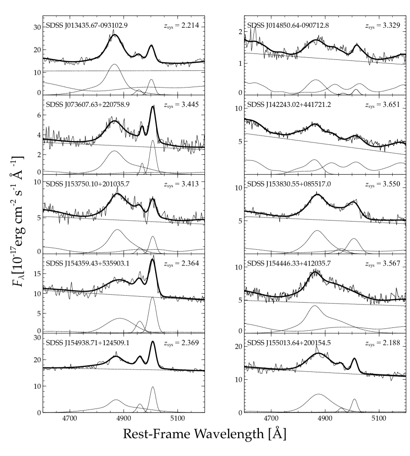
Figure 1.— NIR spectra of $2.15<z<3.70$ quasars. The spectrum in each panel is given by a thin solid line. The fit to each individual feature, Fe ii, H$\beta$, and [O iii] where applicable, and the linear continuum are indicated by dashed lines. The overall fit to each spectrum is given by the bold solid line.

[h]

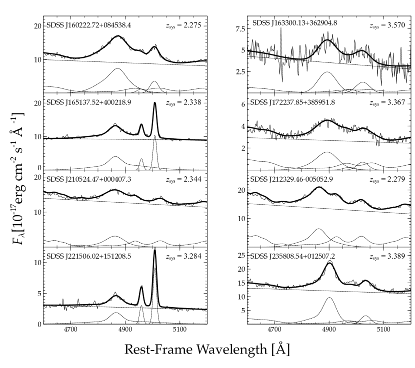
Figure 1.— (Continued.)

2. Sample Selection, Observations, and Data Analysis

We have selected a sample of 18 quasars for our investigation based upon the following criteria:

1. Availability of a flux-calibrated optical spectrum from the SDSS recorded in the Data Release 10 quasar catalog (Pâris et al., 2014).

2. Brightness in the range $m_{i}<18.5$ in order to keep the signal-to-noise (S/N) ratio of the H$\beta$ region of the respective NIR spectrum, obtained with a 3.8 m telescope, at $\approx 40$.

3. Redshift within one of the following intervals, $2.15~{}<~{}z~{}<~{}2.65$ and $3.20<z<3.70$, in which, at a minimum, the H$\beta$ and [O iii] lines can be modeled accurately within one of the near-infrared transmission windows in the $H$ or $K$ bands.

Table 2Spectral Measurements of the H$\beta$ Region and H$\alpha$

	FWHMH$\beta$	EWH$\beta$	$\lambda$peak H$\beta$	FWHM[O iii]	EW[O iii]	$\lambda$peak [O iii]	FWHMH$\alpha$	EWH$\alpha$	$\lambda$peak H$\alpha$
Quasar	(km s-1)	(Å)	(Å)	(km s-1)	(Å)	(Å)	(km s-1)	(Å)	(Å)
SDSS J013435.67$-$093102.9	4438	99.7	15656	1625	14.6	16091	2882	444	21125
SDSS J014850.64$-$090712.8	4716	33.7	21035	1513	4.3	21680	$\cdots$	$\cdots$	$\cdots$
SDSS J073607.63$+$220758.9	6876	94.3	21625	1640	31.6	22256	$\cdots$	$\cdots$	$\cdots$
SDSS J142243.02$+$441721.2	4563	39.9	22607	$\cdots$	$\cdots$	$\cdots$	$\cdots$	$\cdots$	$\cdots$
SDSS J153750.10$+$201035.7	5107	69.5	21516	1613	14.6	22094	$\cdots$	$\cdots$	$\cdots$
SDSS J153830.55$+$085517.0	5512	70.8	22161	3192	26.1	22782	$\cdots$	$\cdots$	$\cdots$
SDSS J154359.43$+$535903.1	8301	54.3	16495	1835	28.6	16843	7495	543	22171
SDSS J154446.33$+$412035.7	7235	132.4	22202	$\cdots$	$\cdots$	$\cdots$	$\cdots$	$\cdots$	$\cdots$
SDSS J154938.71$+$124509.1	5495	42.4	16408	1544	15.4	16866	5550	374	22139
SDSS J155013.64$+$200154.5	6539	61.9	15544	1325	7.5	15960	5178	391	20962
SDSS J160222.72$+$084538.4	6676	122.3	15951	2387	19.5	16398	5629	586	21517
SDSS J163300.13$+$362904.8	4876	57.8	22297	3768	24.6	22884	$\cdots$	$\cdots$	$\cdots$
SDSS J165137.52$+$400218.9	4405	65.6	16234	957.8	18.5	16713	4380	377	21920
SDSS J172237.85$+$385951.8	5938	67.9	21300	3028	13.9	21866	$\cdots$	$\cdots$	$\cdots$
SDSS J210524.47$+$000407.3	5331	25.3	16256	$\cdots$	$\cdots$	$\cdots$	4530	281	21975
SDSS J212329.46$-$005052.9	4500	48.1	15929	$\cdots$	$\cdots$	$\cdots$	4084	319	21540
SDSS J221506.02$+$151208.5	4059	100.0	20840	956.9	61.7	21450	$\cdots$	$\cdots$	$\cdots$
SDSS J235808.54$+$012507.2	3702	63.3	21397	2652	11.6	21974	$\cdots$	$\cdots$	$\cdots$

Spectroscopic observations of this sample were performed at the United Kingdom Infrared Telescope (UKIRT) on Mauna Kea, Hawaii. The observation log and quasar basic properties appear in Table 1.
We utilized the UKIRT Imager-Spectrometer (UIST) with a slit width of 0.24″ to maximize the resolution at the expense of potentially higher slit losses. During these observations, the telescope was nodded in an ABBA pattern in order to obtain primary background subtraction. The broad band B2 filter was used in order to obtain a wavelength range of approximately $1.395-2.506~{}\mu$m, spanning the $H$ and $K$ bands as necessary. The dispersion for these observations was $10.9$ Å pixel^-1 with a spectral resolution of $R\sim 448$. Standard stars of spectral type G and F were observed on each night alongside the quasar in order to remove the telluric features that are present in the quasars’ spectra.
The two-dimensional spectra of the quasars and the standard stars were obtained using standard IRAF routines. Each of the objects was initially pair subtracted in order to remove most of the background noise. Then, both the positive and negative residual peaks were analyzed and averaged together. During the analysis, wavelength calibration was achieved using Argon arc lamps. The hydrogen features in each standard star were removed prior to removing the telluric features from the quasars’ spectra.
Removal of the telluric features and the instrumental response from the quasar spectra was done by dividing these spectra by their respective standard star spectra. Then, any remaining cosmic ray signatures on the quasar spectra were carefully removed. Final, flux calibrated quasar spectra were obtained by multiplying these data by blackbody curves with temperatures corresponding to the spectral types of the telluric standards and by a constant factor that was determined by comparing the $H$, for $2.15<z<2.65$, or $K$, for $3.20<z<3.70$, band magnitudes from the Two Micron All Sky Survey (2MASS; Skrutskie et al., 2006) to the integrated flux across the respective band using the flux conversion factors from Table A.2 of Bessell et al. (1998). We do not rely on the telluric standards for the purpose of flux calibration given the relatively narrow slit and the differences in atmospheric conditions between the observations of the quasars and their respective standard stars. For each source, we utilized their SDSS spectrum to verify that the combined SDSS and UKIRT spectra are consistent with a typical quasar optical-UV continuum of the form $\text{f}_{\nu}\propto\nu^{-0.5}$ (Vanden Berk et al., 2001). By comparing the flux densities at the rest-frame wavelength of 5100 Å to the flux densities at the rest-frame wavelength in the region of 2000 to 3500 Å, dependent on the redshift, in the SDSS spectrum of each source, we verified that the differences between the two values were within $30\%$, indicating, at most, only modest flux variations. Such variations, over a temporal baseline of $\sim 6$ years in the rest-frame are not atypical for such luminous quasars, even if most of these variations are intrinsic as opposed to measurement errors (see, e.g., Kaspi et al., 2007).

2.1. Fitting of the UKIRT Spectra

In order to fit the H$\beta$ and H$\alpha$ spectral regions, we used a model consisting of a local, linear continuum, which is a good approximation to a power-law continuum given the relatively narrow spectral band, a broadened Boroson & Green (1992) Fe ii emission template, and a multi-Gaussian fit to the emission lines. The Fe ii template was broadened by a FWHM value that was free to vary between $2000$ and $10000$ km s^-1 and, along with the linear continuum, was removed to more accurately fit the H$\beta$ and [O iii] emission lines. The chosen FWHM to broaden the Fe ii template was determined with a least squares analysis.
We fit the H$\beta$ line using two independent Gaussians, constrained by the width and height of the emission line, simultaneously with one Gaussian for each of the [O iii] emission lines. The Gaussians assigned to the [O iii] emission lines have identical widths and their intensity ratio was fixed to $I($[O iii] $\lambda 5007)/I($[O iii] $\lambda 4959)=3$. The wavelengths of the two [O iii] components were fixed to the ratio 5007/4959. For the available H$\alpha$ features, two Gaussians were fit after a linear continuum was fit and subtracted around the emission line. We do not detect any [N ii] emission lines while fitting this region, mainly given our low spectral resolution. The Gaussians were constrained so that the line peak would lie within 1,500 km s^-1 from the wavelength that corresponded to the maximum of the emission line region, the widths could range from 0 km s^-1 to 15,000 km s^-1, and the flux density was restricted to lie within 0 and twice the maximum value of the emission line.

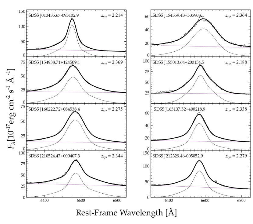
Figure 3.— NIR spectra of $2.15<z<2.65$ quasars. The spectrum in each panel is given by a thin solid line. The fit to the H$\alpha$ line and linear continuum are indicated by dashed lines. The overall fit to each spectrum is given by the bold solid line.

To estimate the uncertainties on the FWHM and rest-frame equivalent width (EW) of the emission lines, we performed the fitting by adjusting the placement of the continuum according to the noise level in the continuum (see, e.g., Shemmer & Lieber, 2015). Namely, by adjusting the local linear continuum between extremes of the noise around each emission line, we were able to derive an estimate for uncertainties on the FWHM and EW values. For all but two of the sources, the uncertainties on the values of FWHM and EW in the H$\beta$ region are on the order of $\sim 5$-$15\%$. For SDSS J014850.64$-$090712.8 and SDSS J163300.13$+$362904.8, these uncertainties are on the order of $\sim 40\%$. Similarly, the uncertainties on the FWHM and EW values for the H$\alpha$ emission line are up to $\sim 5\%$.
The uncertainties on the wavelengths of the peaks of all the emission lines are up to $\sim 300$ km s^-1. The majority of this uncertainty arises from the resolution of our spectrograph, however, our choice of a narrow slit was used to combat this. The uncertainty introduced from the pixel-wavelength calibration is minimal, averaging $\sim 5$ km s^-1. The narrow [O iii] $\lambda 5007$ emission line provided our most accurate redshift estimates, having uncertainties on wavelength measurements averaging $\sim 150$ km s^-1. The wavelength uncertainties were determined by evaluating our S/N ratio and repeated measurements of each of the emission lines.
Basic spectral properties resulting from those fits are reported in Table 2. Columns (2), (3), and (4) provide the FWHM, EW, and the observed-frame wavelength of the peak ($\lambda_{\rm peak}$) of the H$\beta$ line, respectively. Columns (5–7) and (8–10) provide similar information for the [O iii] $\lambda 5007$ and H$\alpha$ emission lines, respectively. The fits for the H$\beta$ and [O iii] emission lines appear in Figure 1, and the fits for the H$\alpha$ emission line appear in Figure 3.

2.2. Spectral Fitting of the C iv Emission Lines

In order to provide corrections to the UV-based redshifts of our sources, we fit the C iv emission lines present in their SDSS spectra. These fits appear in Figure 4. As suggested in M17, the parameters needed for the correction of the UV-based redshifts are the FWHM and EW of the C iv line, as well as the monochromatic luminosity of the continuum at a rest-frame wavelength of $1350$ Å.
The C iv emission line was fit with a local, linear continuum and two independent Gaussians under the same constraints as we report for the H$\beta$ and H$\alpha$ emission lines. The spectral properties resulting from this fitting procedure are reported in Table 3. The uncertainties in each of these measurements were determined by the same method used when evaluating the rest-frame optical emission line uncertainties. Along with this fit, the continuum luminosity, $L_{1350}$, has also been derived by measuring the continuum flux density at rest-frame $\lambda 1350$ Å and employing our chosen cosmology. These values also appear in Table 3.

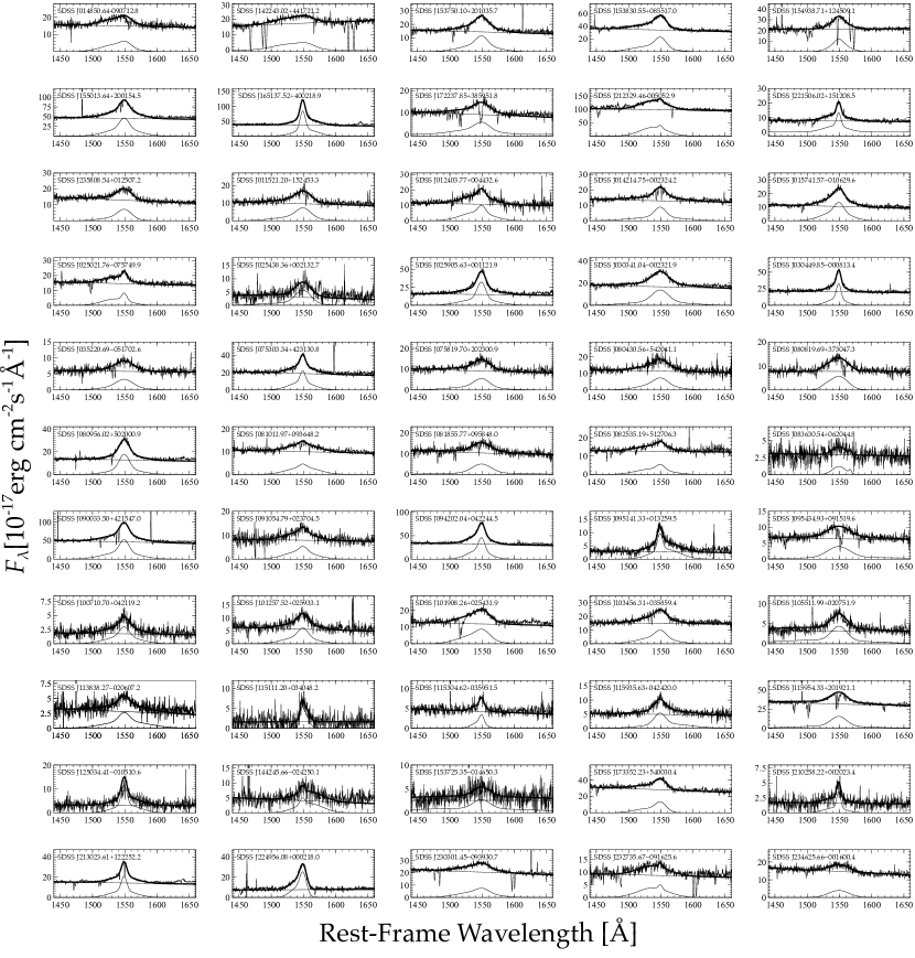
Figure 4.— C iv fits of all 55 quasars used in the regression analysis. The spectrum and fit to the C iv emission line in each panel are given by a thin solid line. The linear continuum is indicated by a dashed line. The overall fit to each spectrum is given by the bold solid line.

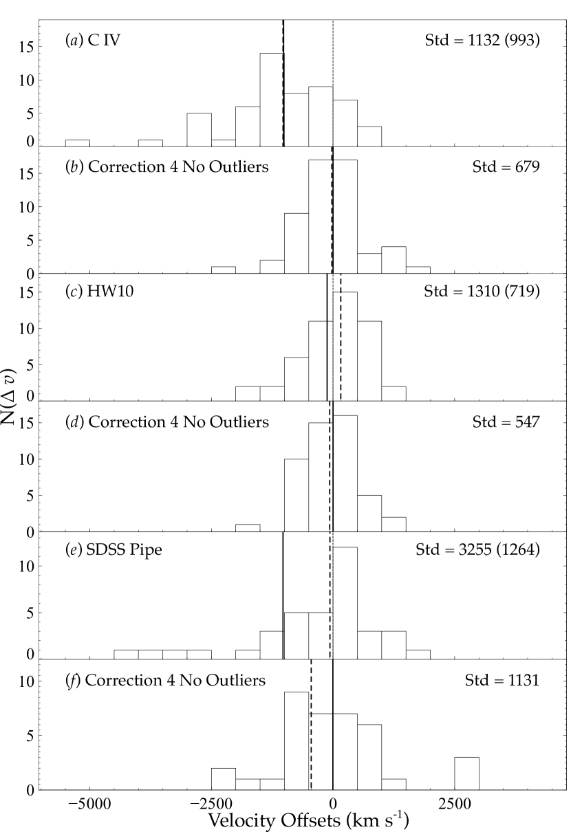
Figure 5.— Velocity offsets relative to $z_{\rm sys}$ before (panels a, c, and e) and after (panels b, d, and f) the correction provided in bold face in Table 7. The numbers reported in parentheses are the standard deviations of the original distributions without the outliers. The mean (solid line) and median (dashed line) are marked in each panel. SDSS J142243.02$+$441721.2 does not appear on the SDSS Pipe panel, for clarity, because of its abnormally large velocity offset. The outliers that were removed are discussed in Section 4.

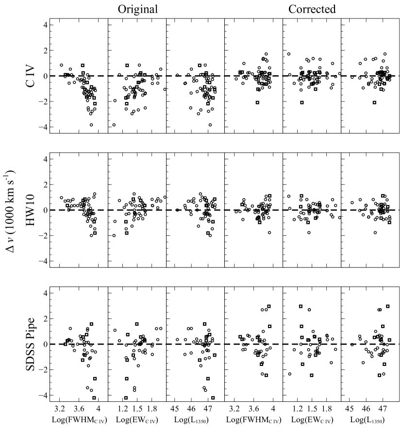
Figure 6.— The residual velocity offsets with respect to $z_{\rm sys}$ before, three leftmost panels, and after, three rightmost panels, correction are presented against our regression parameters. The corrected method displayed refers to Correction 4 without outliers reported in Table 7. Squares (circles) represent data from M17 (UKIRT; this work). The outliers discussed in Section 3.1 do not appear in this plot given their abnormally large velocity offsets.

Table 3Spectral Measurements of C iv

	FWHM	EW	log $L_{1350}$	FWHM	EW	log $L_{1350}$	$\lambda_{\rm peak}$
Quasar Name	(km s-1)	(Å)	(erg s-1)	(km s-1)	(Å)	(erg s-1)	(Å)
SDSS J013435.67$-$093102.9	1045	$\cdots$	$\cdots$	$\cdots$	$\cdots$	$\cdots$	$\cdots$
SDSS J014850.64$-$090712.8	9545	16.3	47.0	8490	19.2	47.0	6657
SDSS J073607.63$+$220758.9	$\cdots$	$\cdots$	$\cdots$	2496	10.0	46.8	6872
SDSS J142243.02$+$441721.2	12475	20.8	47.0	12326	17.9	47.0	7082
SDSS J153750.10$+$201035.7	6080	37.9	47.1	5886	33.3	47.1	6824
SDSS J153830.55$+$085517.0	5754	27.1	47.5	5279	26.2	47.4	7023
SDSS J154359.43$+$535903.1	4713	42.6	47.0	4553	36.9	46.9	5211
SDSS J154446.33$+$412035.7	15266	192.3	46.3	7350	34.4	46.6	7001
SDSS J154938.71$+$124509.1	4207	24.2	46.6	4740	19.6	46.5	5233
SDSS J155013.64$+$200154.5	4273	42.6	47.0	4858	37.4	46.9	4942
SDSS J160222.72$+$084538.4	4150	27.8	47.0	5615	30.7	47.0	5065
SDSS J163300.13$+$362904.8	6963	34.9	46.9	6614	42.0	46.8	7067
SDSS J165137.52$+$400218.9	2818	49.9	46.9	2297	45.2	46.9	5172
SDSS J172237.85$+$385951.8	$\cdots$	$\cdots$	$\cdots$	7208	31.1	46.8	6745
SDSS J210524.47$+$000407.3	12603	36.4	47.1	7990	11.9	46.8	5098
SDSS J212329.46$-$005052.9	8549	16.2	47.4	8168	18.5	47.3	5050
SDSS J221506.02$+$151208.5	$\cdots$	$\cdots$	$\cdots$	2094	35.8	46.7	6638
SDSS J235808.54$+$012507.2	$\cdots$	$\cdots$	$\cdots$	5728	20.2	47.1	6761

3. Results

Combined with the sources in M17, we have a total of 63 objects in our sample, of which, six of our UKIRT objects were excluded from further analysis due to broad absorption line (BAL) identification: these are noted in Table 1. We then remove an additional BAL quasar, SDSS J014049.18$-$083942.5, from the sample in M17. Furthermore, we have excluded SDSS J013435.67$-$093102.9 from our sample given that it is a lensed quasar and its rest-frame UV spectrum is severely attenuated by the foreground lensing galaxy (see e.g., Ofek et al., 2006). Measurements of the C iv emission line for 52 out of the 55 sources in our combined sample are available in Shen et al. (2011). The C iv FWHM and EW measurements we obtained for 40 of these sources agree to within $\sim 20\%$ with those from Shen et al. (2011); similarly, measurements of 10 of these sources agree to within $\sim 65\%$. Generally, these discrepancies are inversely proportional to the signal-to-noise ratios of the SDSS spectra and are larger in the presence of narrow absorption lines. The spectra for SDSS J025438.36$+$002132.7 and SDSS J153725.35$-$014650.3 had extremely poor signal-to-noise ratios, resulting in discrepancies of $108\%$ and $53\%$ for FWHM, and $57\%$ and $210\%$ for EW, respectively, between our measured values and the ones reported in Shen et al. (2011). Substituting our values with the ones reported in Shen et al. (2011) for these objects did not have a significant impact on further analysis.
The observed-frame wavelength of the peak of the C iv emission line was compared to the value predicted by the systemic redshift ($z_{\rm sys}$) to determine the velocity offset of this line. We determine $z_{\rm sys}$ from the line peak of the emission line with the smallest measurement uncertainty. In order, we take our systemic redshift from [O iii] ($\sim 50$ km s^-1), Mg ii ($\sim 200$ km s^-1) and H$\beta$ ($\sim 400$ km s^-1) (Shen et al., 2016). The C iv velocity offsets are shown and reported in Figure 5 and Table 4, respectively. In Table 4, we also report the redshift measurements provided for these sources in HW10 and Pâris et al. (2018, hereafter P18), where applicable. The velocity offsets introduced from these redshifts with respect to $z_{\rm sys}$ are presented in Figure 5 and Table 4. In addition to the velocity offsets for the sources in our UKIRT sample, the velocity offsets from Table 1 of M17 have been included in the following regression analysis. The C iv emission line properties for the M17 sample are reported in Table 5.
We note that the $\Delta v_{\text{C~{}{\sc iv}}}$ values used in M17 differ from the $\Delta v_{\text{C~{}{\sc iv}}}$ values we compute for the M17 sample since M17 used the $\Delta v_{\text{C~{}{\sc iv}}}$ values from Shen et al. (2011), combined with the redshift determined from the SDSS Pipeline, in order to find $z_{\text{C~{}{\sc iv}}}$. Our $\Delta v_{\text{C~{}{\sc iv}}}$ values follow directly from the measurement of $\lambda_{\rm peak}$ (C iv) and our derived $z_{\rm sys}$. The origin of the discrepancies between the two velocity offsets used stems from the uncertainty in the $\Delta v_{\text{C~{}{\sc iv}}}$ values discussed in Shen et al. (2011). The differences between the $\Delta v_{\text{C~{}{\sc iv}}}$ values we use and those used by M17 are rather small, and using the latter values do not change our results significantly.
A multiple regression analysis has been performed on the velocity offsets and the C iv emission line properties such that:

$$\begin{split}\Delta v~{}(\text{km}~{}\text{s}^{-1})=\alpha\log_{10}(\text{FWHM}_{\text{C~{}{\sc iv}}})\\ +\beta\log_{10}(\text{EW}_{\text{C~{}{\sc iv}}})+\gamma\log_{10}(L_{1350})\end{split}$$ (1)

where $\Delta v$ is the velocity offset and $\alpha$, $\beta$, and $\gamma$ are the coefficients associated with our regression analysis. The velocity offset created by each redshift derivation method was determined by the following equation

$$\begin{split}\Delta v=c\bigg{(}\frac{z_{\rm meas}-z_{\rm sys}}{1+z_{\rm sys}}\bigg{)}.\end{split}$$ (2)

Where $z_{\rm meas}$ is the redshift derived using various methods and reported in the studies indicated below. In order to derive the most reliable redshift correction, four regressions were performed using the following parameters from Equation 1:

1. $\log_{10}(\text{FWHM}_{\text{C~{}{\sc iv}}})$, $\log_{10}(\text{EW}_{\text{C~{}{\sc iv}}})$

2. $\log_{10}(\text{FWHM}_{\text{C~{}{\sc iv}}})$, $\log_{10}(L_{1350})$

3. $\log_{10}(\text{EW}_{\text{C~{}{\sc iv}}})$, $\log_{10}(L_{1350})$

4. All three parameters

In total, this regression analysis was performed on redshifts determined from: 1) the measured line peak of the C iv emission line, 2) HW10, and 3) the SDSS Pipeline. The coefficients, errors, and confidence statistics from Equation 1, determined in each of these cases, are reported in Table 6. For the confidence statistics, we report the $t$-Value (e.g., Sheskin, 2007) to determine the importance of each individual parameter.
The residuals of the velocity offsets after each correction has been determined have been analyzed, and basic statistics resulting from these residuals are listed in Table 7. The residuals before and after correction are presented in Figure 6. The residual distributions show the significant reduction in the velocity offsets before and after each correction. The corrected velocity offsets for C iv- and HW10-based redshifts are closer to zero than the corrected velocity offsets for the SDSS Pipeline-based redshift, representative of the larger $\sigma$ value associated with SDSS Pipeline redshift estimates. From evaluating the best fitting coefficients and statistics reported for each correction, we determined the correction that we consider to provide the most reliable results. This correction has been emphasized in bold face in the text.

3.1. SDSS J142243.02$+$441721.2 and SDSS J115954.33$+$201921.1

SDSS J142243.02$+$441721.2 from our UKIRT sample has significantly larger velocity offsets compared to the rest of the combined sample. The velocity offsets determined from C iv, HW10, and SDSS Pipeline are $-5097$ km s^-1, $-7740$ km s^-1, and $-16384$ km s^-1, respectively. The latter velocity offset stems from a misidentification of spectral features in the SDSS spectrum of the source as manifested by the SDSS Pipeline products. The SDSS Pipeline redshift for this source is $z=3.396$ while the SDSS Visual Inspection value is $z=3.615$. The disparity between these estimates confirms the misidentification of the emission lines by the SDSS Pipeline. Because the velocity offsets for this source had a significant impact on the regression analysis and may be misleading, we have provided the results of the regression analysis with and without this object in Table 7.
The velocity offset of SDSS J115954.33$+$201921.1 from the M17 sample, with respect to the redshift determined by the SDSS Pipeline is $-10642$ km s^-1, which is significantly larger than the respective values of the combined sample, excluding SDSS J142243.02$+$441721.2. SDSS J115954.33$+$201921.1 was also removed from the SDSS Pipeline regression as discussed further in Section 4. Here too, the disparity between the SDSS Pipeline redshift value ($z=3.330$) and the respective Visual Inspection value ($z=3.425$) indicates a misidentification of spectral features by the SDSS Pipeline.

Table 4Redshift Comparison

		$\Delta v$		$\Delta v$		$\Delta v$
Quasar	$z_{\rm\text{C~{}{\sc iv}}}\tablenotemark{a}$	(km s-1)	$z_{\rm pipe}\tablenotemark{b}$	(km s-1)	$z_{\rm HW10}\tablenotemark{c}$	(km s-1)
SDSS J013435.67$-$093102.9	2.214	$\cdots$	$\cdots$	$\cdots$	2.225	1029
SDSS J014850.64$-$090712.8	3.274	-3786	3.290	-2691	3.303	-1796
SDSS J073607.63$+$220758.9	3.436	-607	3.464	1285	$\cdots$	$\cdots$
SDSS J142243.02$+$441721.2	3.572	-5097	3.397	-16384	3.531	-7740
SDSS J153750.10$+$201035.7	3.405	-544	$\cdots$	$\cdots$	$\cdots$	$\cdots$
SDSS J153830.55$+$085517.0	3.535	-989	3.537	-856	3.563	858
SDSS J154359.43$+$535903.1	2.365	89	2.370	536	2.379	1341
SDSS J154446.33$+$412035.7	3.520	-3087	3.569	131	3.551	-1049
SDSS J154938.71$+$124509.1	2.378	801	2.355	-1244	$\cdots$	$\cdots$
SDSS J155013.64$+$200154.5	2.190	188	2.194	565	2.196	754
SDSS J160222.72$+$084538.4	2.270	-458	$\cdots$	$\cdots$	2.276	92
SDSS J163300.13$+$362904.8	3.562	-525	3.538	-2093	3.575	328
SDSS J165137.52$+$400218.9	2.339	90	2.341	270	2.342	360
SDSS J172237.85$+$385951.8	3.350	-1168	3.390	1584	$\cdots$	$\cdots$
SDSS J210524.47$+$000407.3	2.293	-4575	$\cdots$	$\cdots$	2.307	-3301
SDSS J212329.46$-$005052.9	2.255	-1376	2.233	-3395	2.269	-92
SDSS J221506.02$+$151208.5	3.285	70	3.284	0	$\cdots$	$\cdots$
SDSS J235808.54$+$012507.2	3.366	-1572	3.400	753	$\cdots$	$\cdots$

Table 5C iv Spectral Properties of the M17 Sample

			FWHM	EW	log $L_{1350}$	$\lambda_{\rm peak}$
Quasar	$z_{\rm HW10}$	$z_{\rm pipe}$	(km s-1)	(Å)	(erg s-1)	(Å)
SDSS J011521.20$+$152453.3	3.433	3.418	6236	33.3	46.6	6821
SDSS J012403.77$+$004432.6	3.827	3.836	5646	37.4	47.1	7460
SDSS J014049.18$-$083942.5	3.726	$\cdots$	4635	22.7	47.2	7285
SDSS J014214.75$+$002324.2	3.374	$\cdots$	5013	29.2	47.0	6753
SDSS J015741.57$-$010629.6	3.571	3.565	5158	45.9	46.9	7049
SDSS J025021.76$-$075749.9	3.344	3.337	5173	18.8	47.0	6715
SDSS J025438.36$+$002132.7	2.464	2.470	5998	78.8	45.8	5355
SDSS J025905.63$+$001121.9	3.377	3.372	3728	65.6	46.9	6767
SDSS J030341.04$-$002321.9	3.235	$\cdots$	6865	41.0	47.0	6524
SDSS J030449.85$-$000813.4	3.296	$\cdots$	2066	27.1	47.3	6638
SDSS J035220.69$-$051702.6	3.271	$\cdots$	6939	24.7	46.4	6578
SDSS J075303.34$+$423130.8	3.595	3.594	2804	29.4	47.3	7112
SDSS J075819.70$+$202300.9	3.753	3.743	6583	27.6	46.8	7333
SDSS J080430.56$+$542041.1	3.755	3.758	7047	28.7	46.8	7335
SDSS J080819.69$+$373047.3	3.477	3.426	7183	27.8	46.9	6910
SDSS J080956.02$+$502000.9	3.288	3.290	4240	41.9	47.0	6623
SDSS J081011.97$+$093648.2	3.387	$\cdots$	7558	21.3	46.9	6768
SDSS J081855.77$+$095848.0	3.688	3.692	7446	26.9	47.0	7213
SDSS J082535.19$+$512706.3	3.507	3.496	6839	18.7	47.1	6964
SDSS J083630.54$+$062044.8	3.387	3.413	5971	11.0	47.1	6767
SDSS J090033.50$+$421547.0	3.294	3.296	4421	40.3	47.3	6639
SDSS J091054.79$+$023704.5	3.290	3.292	6184	27.7	46.4	6618
SDSS J094202.04$+$042244.5	3.284	3.272	3208	35.0	46.9	6617
SDSS J095141.33$+$013259.5	2.419	2.425	2645	96.5	46.0	5293
SDSS J095434.93$+$091519.6	3.398	3.399	8671	41.1	46.7	6802
SDSS J100710.70$+$042119.2	2.367	2.354	4988	64.8	45.6	5199
SDSS J101257.52$+$025933.1	2.441	2.436	5106	39.9	46.1	5312
SDSS J101908.26$+$025431.9	3.379	$\cdots$	8012	34.5	47.0	6766
SDSS J103456.31$+$035859.4	3.388	3.342	5972	27.8	46.8	6767
SDSS J105511.99$+$020751.9	3.404	$\cdots$	6372	84.5	46.1	6798
SDSS J113838.27$-$020607.2	3.347	3.342	5888	46.4	46.0	6711
SDSS J115111.20$+$034048.2	2.337	2.341	2448	44.8	45.2	5170
SDSS J115304.62$+$035951.5	3.437	3.430	2379	13.6	46.6	6858
SDSS J115935.63$+$042420.0	3.456	3.457	4969	44.8	46.3	6886
SDSS J115954.33$+$201921.1	3.432	3.269	6360	24.8	47.4	6827
SDSS J125034.41$-$010510.6	2.399	2.401	2494	83.7	45.6	5252
SDSS J144245.66$-$024250.1	2.355	$\cdots$	6176	46.2	46.0	5155
SDSS J153725.35$-$014650.3	3.467	$\cdots$	8098	117.7	46.7	6872
SDSS J173352.23$+$540030.4	3.435	$\cdots$	4994	17.1	47.4	6844
SDSS J210258.22$+$002023.4	3.342	$\cdots$	1733	35.0	46.8	6723
SDSS J213023.61$+$122252.2	3.279	$\cdots$	2596	33.6	47.0	6615
SDSS J224956.08$+$000218.0	3.323	3.309	2994	64.0	46.8	6677
SDSS J230301.45$-$093930.7	3.470	$\cdots$	8425	18.7	47.3	6898
SDSS J232735.67$-$091625.6	3.470	$\cdots$	8378	27.3	46.5	6582
SDSS J234625.66$-$001600.4	3.281	$\cdots$	7172	10.5	47.1	6892

Note. — The $z_{\rm sys}$ values used in determining the velocity offsets are reported in Column 3 of Table 1 in M17.

Table 6Correction Coefficients

Correction	Equation	Coefficients	Value	Error	$t$-Value
C iv	$\alpha\log_{10}(\text{FWHM}_{\text{C~{}{\sc iv}}})+\beta\log_{10}(\text{EW}_{\text{C~{}{\sc iv}}})$	$\alpha$	-1301	195	-6.68
		$\beta$	2501	472	5.29
	$\alpha\log_{10}(\text{FWHM}_{\text{C~{}{\sc iv}}})+\gamma\log_{10}(L_{1350})$	$\alpha$	-3966	600	-6.61
		$\gamma$	293	48	6.14
	$\beta\log_{10}(\text{EW}_{\text{C~{}{\sc iv}}})+\gamma\log_{10}(L_{1350})$	$\beta$	2058	601	3.43
		$\gamma$	-88	20	-4.50
	$\alpha\log_{10}(\text{FWHM}_{\text{C~{}{\sc iv}}})+\beta\log_{10}(\text{EW}_{\text{C~{}{\sc iv}}})+\gamma\log_{10}(L_{1350})$	$\alpha$	-3670	549	-6.68
		$\beta$	1604	450	3.57
		$\gamma$	217	48	4.53
HW10	$\alpha\log_{10}(\text{FWHM}_{\text{C~{}{\sc iv}}})+\beta\log_{10}(\text{EW}_{\text{C~{}{\sc iv}}})$	$\alpha$	-1069	254	-4.22
		$\beta$	2517	612	4.11
	$\alpha\log_{10}(\text{FWHM}_{\text{C~{}{\sc iv}}})+\gamma\log_{10}(L_{1350})$	$\alpha$	-3191	869	-3.67
		$\gamma$	251	69	3.63
	$\beta\log_{10}(\text{EW}_{\text{C~{}{\sc iv}}})+\gamma\log_{10}(L_{1350})$	$\beta$	2219	715	3.10
		$\gamma$	-75	24	-3.18
	$\alpha\log_{10}(\text{FWHM}_{\text{C~{}{\sc iv}}})+\beta\log_{10}(\text{EW}_{\text{C~{}{\sc iv}}})+\gamma\log_{10}(L_{1350})$	$\alpha$	-2834	819	-3.46
		$\beta$	1877	652	2.88
		$\gamma$	161	71	2.26
SDSS Pipe	$\alpha\log_{10}(\text{FWHM}_{\text{C~{}{\sc iv}}})+\beta\log_{10}(\text{EW}_{\text{C~{}{\sc iv}}})$	$\alpha$	-2380	785	-3.03
		$\beta$	5087	1891	2.69
	$\alpha\log_{10}(\text{FWHM}_{\text{C~{}{\sc iv}}})+\gamma\log_{10}(L_{1350})$	$\alpha$	-8024	2732	-2.94
		$\gamma$	613	216	2.83
	$\beta\log_{10}(\text{EW}_{\text{C~{}{\sc iv}}})+\gamma\log_{10}(L_{1350})$	$\beta$	4732	2240	2.11
		$\gamma$	-176	74	-2.39
	$\alpha\log_{10}(\text{FWHM}_{\text{C~{}{\sc iv}}})+\beta\log_{10}(\text{EW}_{\text{C~{}{\sc iv}}})+\gamma\log_{10}(L_{1350})$	$\alpha$	-6814	2830	-2.41
		$\beta$	3114	2212	1.41
		$\gamma$	416	255	1.63

4. Discussion

The results of our multiple regression analysis indicate that the most reliable redshift is obtained by correcting the HW10-based redshift employing the FWHM and EW of the C IV line, the monochromatic luminosity at rest-frame 1350 Å, and the respective coefficients listed under the fourth correction to the HW10 method from Table 6. Using this correction, and removing SDSS J142243.02$+$441721.2 from the analysis (see Sec. 3.1), we were able to reduce the uncertainty on the redshift determination from 731 km s^-1 to 543 km s^-1, yielding an improvement of $\sim 25\%$ with respect to the HW10-based redshifts; similarly, the mean systematic offset of the redshift determination is reduced from $-137$ km s^-1 to $+1$ km s^-1 (see Table 7). For comparison, utilizing only the M17 sample of 44 sources, the uncertainty on the HW10-based redshifts is reduced by $\sim 20\%$. The addition of the five sources from our UKIRT sample that have HW10-based redshifts, comprising a $\sim 10\%$ increase in the number of sources with respect to the M17 sample, therefore helped to further reduce the uncertainty on the HW10-based redshifts from $\sim 20\%$ to $\sim 25\%$. We anticipate that by utilizing a more representative of several hundred high-redshift quasars, we will be able to further improve these uncertainties significantly and the results will become increasingly less biased to small number statistics (e.g., Matthews et al., in prep.).
We note that, when we include the source with the highly discrepant $\Delta v_{\text{C~{}{\sc iv}}}$ value, SDSS J142243.02$+$441721.2, in the regression analysis, the best redshift estimates are obtained from the corrected C iv-based redshifts (see Table 7). In this case, the mean systematic redshift offsets reduces from $-1023$ km s^-1 to $-8$ km s^-1 and the uncertainty on the redshifts determination decreases from 1135 km s^-1 to 746 km s^-1 (a $\sim 34\%$ improvement).
As it is apparent, even with this sample of 55 quasars, the methods to determine redshift using rest-frame UV features provide uncertainties as large as $\approx 500-700$ km s^-1. As reported in the first row of each section of Table 7, the uncorrected redshift determinations are significantly inaccurate and imprecise. C iv-based redshifts have a mean systematic offset of $\sim 1000$ km/s (a blueshift) and a similar value for $\sigma$ (the standard deviation). The HW10 method further improves these C iv-based redshifts by reducing the systematic offsets by $\sim 900$ km s^-1 and $\sigma$ by $\sim 300$ km s^-1. Our prescription further reduces the systematic offset by an additional $\sim 100$ km s^-1 and reduces $\sigma$ by an additional $\sim 200-300$ km s^-1. Using the SDSS Pipeline redshift estimate, determined from a principal component analysis on multiple features of a spectrum simultaneously (e.g., Bolton et al., 2012), the mean systematic velocity offset for our combined sample is the largest and extends beyond $1000$ km s^-1 with a standard deviation of $1324$ km s^-1. Overall, albeit utilizing a smaller combined sample with respect to the samples we use for C iv- and HW10-based redshifts, the redshifts determined from the SDSS Pipeline provide the least reliable results (see Table 7). Our best correction applied to these redshifts improves the mean systematic velocity offset by $\sim 1000$ km s^-1, similar to the improvement achieved for C iv-based redshifts, but yields only a modest improvement in $\sigma$ which remains large.
In order to test the validity of our method, we have preformed the same regression described in the text on the M17 sources ($\sim 80\%$ of our combined sample) and applied it to the remaining sources acquired from UKIRT. The C iv velocity offsets were used in the regression since this sample was the largest of the three UV-based redshift estimates. Prior to correction, the sample of 10 UKIRT sources had a mean, median and $\sigma$ of $-641$ km s^-1, $-690$ km s^-1, and $952$ km s^-1 respectively. After running the regression on the M17 sample and applying the new correction to the UKIRT sources, the mean, median and $\sigma$ improved to $474$ km s^-1, $376$ km s^-1, and $772$ km s^-1 respectively, demonstrating the validity of our method.
The SDSS Pipeline redshift estimate, as noted in P18, is subject to highly uncertain redshift determinations due to lower signal-to-noise ratios or unusual objects. As seen in our relatively small sample, large redshift discrepancies are apparent particularly in two of the 39 objects that we have with available SDSS Pipeline-based redshifts. In each case, the velocity offsets are $>10^{4}$ km s^-1 and, when included in the regression analysis, it nearly tripled the uncertainty on the redshift determination. The most robust redshift determination methods involve a correction based on the C iv spectral properties and UV continuum luminosity to either C iv- or HW10-based redshifts. P18 also provides a redshift based off of visual inspection, $z_{\rm VI}$. We find that this estimate, where available, provides a much more reliable redshift estimate than the one provided by the SDSS Pipeline. The mean systematic offset for this redshift estimate is $-290$ km s^-1 with a standard deviation of $762$ km s^-1.
Regarding the two sources with extremely large velocity offsets, SDSS J142243.02$+$441721.2 and SDSS J115954.33$+$201921.1, we note that our best corrections for their UV-based redshifts provide only modest improvements to the redshift determinations, and that their negative velocity offsets (i.e., blueshifts) take on positive velocity offsets (i.e., redshifts), after the correction is applied. The velocity offsets for SDSS J142243.02$+$441721.2 improve from $-5097$ km s^-1 to $2300$ km s^-1, $-7740$ km s^-1 to $6016$ km s^-1, and $-16384$ km s^-1 to $11848$ km s^-1 for C iv-, HW10-, and SDSS Pipeline-based redshift estimates, respectively. Similarly, the velocity offsets for SDSS J115954.33$+$201921.1 changed from $-1264$ km s^-1 to $-58$ km s^-1, $407$ km s^-1 to $-656$ km s^-1, and $-10642$ km s^-1 to $8720$ km s^-1, respectively. While most of the corrected velocity offsets are closer to zero, they do not improve appreciably and still affect the statistics significantly.
The origin for the abnormally large velocity offset of the SDSS Pipeline redshift of SDSS J115954.33$+$201921.1 most likely stems from the misidentification of the emission lines in the SDSS spectra by the SDSS Pipeline, as discussed in 3.1. As for SDSS J142243.02$+$441721.2, the origin of the large velocity offset of the C iv-based redshift is intrinsic to the quasar and this should not be confused with the coincidental abnormally large velocity offset stemming from the failure of the SDSS Pipeline to correctly identify the UV spectral features (see Sec. 3.1). Our measured velocity offset of the C iv line ($-5097$ km s^-1) is consistent, within the errors, with the value reported in Table 6 of Vietri et al. (2018) for the source ($-4670$ km s^-1). Such sources may point to additional spectral parameters that should be taken into account in future prescriptions for UV-based redshift corrections. While such objects may be rare ($\lesssim 5$% in our combined sample), their potential effects on future redshift estimates should be scrutinized to ensure that redshift corrections for the general quasar population are not skewed. The difficulty in correcting the UV-based redshift of SDSS J142243.02$+$441721.2 is also manifested by the HW10-based redshift which is unable to improve the estimate but rather provides a larger velocity offset ($-7740$ km s^-1) with respect to the C iv-based value ($-5097$ km s^-1).
With our combined sample of 55 high-redshift quasars, we verify large velocity offsets between UV-based redshift estimates and $z_{\rm sys}$. Our calibrations to the UV-based redshift estimates can be used to establish more reliable estimates for $z_{\rm sys}$ when working with high-redshift quasars in the optical band. This effort will lead to more reliable constraints on a range of measurements that require precise distances for quasars.

5. Conclusions

In the coming decade, $\approx 10^{6}$ high-redshift ($z\gtrsim 0.8$) quasars will have their redshifts determined through large spectroscopic surveys conducted in the visible band (i.e., rest-frame UV band), e.g., the DESI survey (e.g., Levi et al., 2013; DESI Collaboration et al., 2016). Many of these quasars, at $1.5\lesssim z\lesssim 6.0$, will have the prominent C iv emission line covered in their spectra. The spectral properties of this line can provide a valuable means for correcting UV-based redshifts as we have shown in this work.

Table 7Correction Statistics

Model	Mean	Median	$\sigma$	Skew
C iv	-1016	-1028	1132 (993)	-1.11
C iv 1	-20	-194	885 (792)	0.55
C iv 2	-3	18	837 (755)	0.66
C iv 3	1	-80	1022 (905)	0.67
C iv 4	0	-24	750 (679)	0.37
HW10	-121	159	1310 (719)	-4.09
HW 1	-14	-116	1123 (575)	3.86
HW 2	-2	-97	1157 (638)	3.38
HW 3	1	-73	1195 (621)	3.98
HW 4	1	-68	1067 (547)	3.59
SDSS Pipe	-1029	-63	3255 (1264)	-3.45
Pipe 1	-31	-558	2954 (1161)	2.78
Pipe 2	-8	-578	2928 (1165)	2.66
Pipe 3	-2	-697	3072 (1200)	3.03
Pipe 4	-3	-449	2851 (1131)	2.54

Note. — Bold results are presented in Figure 5. The $\sigma$ reported in parenthesis is the standard deviation once outliers have been removed. For C iv and HW10, only SDSS J142243.02$+$441721.2 was removed. For SDSS Pipe, SDSS J142243.02$+$441721.2 and SDSS J115954.33$+$201921.1 were removed.

Using a sample of 55 quasars, our prescription for correcting UV-based redshifts yields a mean systematic velocity offset which is consistent with zero and further improves the uncertainty on the redshift determination by $\sim 25-35$% with respect to the method of HW10. We also find that UV-based redshifts derived from the SDSS Pipeline provide the least reliable results, and the associated uncertainties with respect to $z_{\rm sys}$ cannot be reduced appreciably. With a larger, uniform sample of high-redshift quasars with NIR spectroscopy (e.g., Matthews et al., in prep.), we plan to improve the reliability of our redshift estimates further and search for additional spectral properties that may further improve these estimates.
We show that the uncertainties on UV-based redshifts for the majority of high-redshift quasars can be reduced considerably by obtaining NIR spectroscopy of a larger sample of sources and using the [O iii]-based systemic redshift to inform a C iv-based regression analysis. The reduction in redshift uncertainties is particularly useful for a range of applications involving accurate cosmological distances.

6. Acknowledgments

We gratefully acknowledge the financial support by National Science Foundation grants AST-1815281 (C. D., O. S.), and AST-1815645 (M. S. B., A. D. M.). A.D.M. was supported by the Director, Office of Science, Office of High Energy Physics of the U.S. Department of Energy under Contract No. DE-AC02-05CH1123 and Award No. DE-SC0019022. This research has made use of the NASA/IPAC Extragalactic Database (NED), which is operated by the Jet Propulsion Laboratory, California Institute of Technology, under contract with the National Aeronautics and Space Administration, as well as NASA’s Astrophysics Data System Bibliographic Services.

References

- Bessell et al. (1998) Bessell, M. S., Castelli, F., & Plez, B. 1998, A&A, 333, 231
- Bolton et al. (2012) Bolton, A. S., Schlegel, D. J., Aubourg, É., et al. 2012, AJ, 144, 144
- Boroson (2005) Boroson, T. 2005, AJ, 130, 381.
- Boroson & Green (1992) Boroson, T. A., & Green, R. F. 1992, ApJS, 80, 109
- Chen et al. (2014) Chen, Z.-F., Qin, Y.-P., Qin, M., et al. 2014, The Astrophysical Journal Supplement Series, 215, 12.
- DESI Collaboration et al. (2016) DESI Collaboration, Aghamousa, A., Aguilar, J., et al. 2016, arXiv e-prints, arXiv:1611.00036
- Font-Ribera et al. (2013) Font-Ribera, A., Arnau, E., Miralda-Escudé, J., et al. 2013, J. Cosmology Astropart. Phys, 5, 018
- Gaskell (1982) Gaskell, C. M. 1982, ApJ, 263, 79
- Gibson et al. (2009) Gibson, R. R., Jiang, L., Brandt, W. N., et al. 2009, ApJ, 692, 758
- Hewett, & Wild (2010) Hewett, P. C., & Wild, V. 2010, MNRAS, 405, 2302.
- Hogg (1999) Hogg, D. W. 1999, arXiv e-prints, astro-ph/9905116
- Hopkins & Elvis (2010) Hopkins, P. F., & Elvis, M. 2010, MNRAS, 401, 7
- Hutchings et al. (2006) Hutchings, J. B., Cherniawsky, A., Cutri, R. M., et al. 2006, AJ, 131, 680.
- Kaspi et al. (2007) Kaspi, S., Brandt, W. N., Maoz, D., et al. 2007, ApJ, 659, 997
- Levi et al. (2013) Levi, M., Bebek, C., Beers, T., et al. 2013, arXiv:1308.0847
- Mason et al. (2017) Mason, M., Brotherton, M. S., & Myers, A. 2017, MNRAS, 469, 4675.
- Ofek et al. (2006) Ofek, E. O., Maoz, D., Rix, H.-W., et al. 2006, The Astrophysical Journal, 641, 70
- Pâris et al. (2014) Pâris, I., Petitjean, P., Aubourg, É., et al. 2014, A&A, 563, A54
- Pâris et al. (2017) Pâris, I., Petitjean, P., Ross, N. P., et al. 2017, A&A, 597, A79
- Pâris et al. (2018) Pâris, I., Petitjean, P., Aubourg, É., et al. 2018, A&A, 613, A51
- Prochaska et al. (2013) Prochaska, J. X., Hennawi, J. F., Lee, K.-G., et al. 2013, ApJ, 776, 136
- Richards et al. (2009) Richards, G. T., Myers, A. D., Gray, A. G., et al. 2009, The Astrophysical Journal Supplement Series, 180, 67.
- Shemmer & Lieber (2015) Shemmer, O., & Lieber, S. 2015, ApJ, 805, 124
- Shen et al. (2011) Shen, Y., Richards, G. T., Strauss, M. A., et al. 2011, ApJS, 194, 45.
- Shen et al. (2016) Shen, Y., Brandt, W. N., Richards, G. T., et al. 2016, ApJ, 831, 7.
- Sheskin (2007) Sheskin, D. J. 2007, Handbook of Parametric and Nonparametric Statistical Procedures, (4th ed.; Chapman & Hall/CRC)
- Schneider et al. (2010) Schneider, D. P., Richards, G. T., Hall, P. B., et al. 2010, AJ, 139, 2360
- Skrutskie et al. (2006) Skrutskie, M. F., Cutri, R. M., Stiening, R., et al. 2006, AJ, 131, 1163.
- Spergel et al. (2007) Spergel, D. N., Bean, R., Doré, O., et al. 2007, ApJS, 170, 377.
- Tytler & Fan (1992) Tytler, D., & Fan, X.-M. 1992, ApJS, 79, 1
- Vanden Berk et al. (2001) Vanden Berk, D. E., Richards, G. T., Bauer, A., et al. 2001, AJ, 122, 549.
- Vietri et al. (2018) Vietri, G., Piconcelli, E., Bischetti, M., et al. 2018, A&A, 617, A81
- York et al. (2000) York, D. G., Adelman, J., Anderson, J. E., Jr., et al. 2000, AJ, 120, 1579
- Zhao et al. (2019) Zhao, G.-B., Wang, Y., Saito, S., et al. 2019, MNRAS, 482, 3497