Storage Space Allocation Strategy for Digital Data with Message Importance

Abstract

This paper mainly focuses on the problem of lossy compression storage from the perspective of message importance when the reconstructed data pursues the least distortion within limited total storage size. For this purpose, we transform this problem to an optimization by means of the importance-weighted reconstruction error in data reconstruction. Based on it, this paper puts forward an optimal allocation strategy in the storage of digital data by a kind of restrictive water-filling. That is, it is a high efficient adaptive compression strategy since it can make rational use of all the storage space. It also characterizes the trade-off between the relative weighted reconstruction error and the available storage size. Furthermore, this paper also presents that both the users’ preferences and the special characteristic of data distribution can trigger the small-probability event scenarios where only a fraction of data can cover the vast majority of users’ interests. Whether it is for one of the reasons above, the data with highly clustered message importance is beneficial to compression storage. In contrast, the data with uniform information distribution is incompressible, which is consistent with that in information theory.

I Introduction

As growing mobile devices such as Internet of things (IoT) devices or smartphones are utilized, the contradiction between limited storage space and sharply increasing data deluge becomes increasingly serious in the era of big data [1, 2]. This exceedingly massive data makes the conventional data storage mechanisms inadequate within a tolerable time, and therefore the data storage is one of the major challenges in big data [3]. Note that, storing all the data becomes more and more dispensable nowadays, and it is also not conducive to reduce data transmission cost [4, 5]. In fact, the data compression storage is widely adopted in many applications, such as IoT [2], industrial data platform [6], bioinformatics [7], wireless networking [8]. Thus, the research on data compression storage becomes increasingly paramount and compelling nowadays.

In the conventional source coding, data compression is gotten by removing the data redundancy, where short descriptions are assigned to most frequent class [9]. Based on it, the tight bounds for lossless data compression is given. In order to further increase the compression rate, we need to use more information. A quintessential example is that we can do source coding with side information [10]. Another possible solution is to compress the data with quiet a few losses first and then reconstruct them with acceptable distortion [11, 12, 13]. In addition, the adaptive compression is adopted extensively. For example, Ref. [14] proposed an adaptive compression scheme in IoT systems, and backlog-adaptive source coding system in age of information is discussed in Ref. [15]. In fact, most previous compression methods achieved the target of compression by means of contextual data or leveraging data transformation techniques [4]. Instead of compressing data based on removing data redundancy or data correlation, as an alternative, this paper will realize this goal by reallocating storage space with taking the importance as the weight in the weighted reconstruction error to minimize the difference between the raw data and the compressed data when used by people.

Generally, users prefer to care about the crucial part of data that attracts their attentions rather than the whole data itself. Moreover, different errors may bring different costs in many real-world applications [16, 17, 18, 19]. To be specific, the distortion in the data that users care about may be catastrophic while the loss of the data that is insignificance for users is usually inessential. Therefore, we can achieve data compression by storing a fraction of data which preserves as much information as possible regarding the data that users care about [21, 20]. This paper also employs this strategy. However, there are subtle but critical differences between the compression storage strategy proposed in this paper with those in Ref. [21, 20]. In fact, Ref. [20] focused on Pareto-optimal data compression, which presents the trade-off between retained entropy and class information. However, this paper puts forward optimal compression storage strategy for digital data from the viewpoint of message importance, and it gives the trade-off between the weighted reconstruction error and the available storage size. Besides, the compression method based on message importance was preliminarily discussed in Ref. [21] to solve the big data storage problem in wireless communications, while this paper will desire to discuss the optimal storage space allocation strategy with limited storage space in general cases based on message importance. Moreover, the constraints are also different. That is, the available storage size is limited in this paper, while the total code length of all the events is given in Ref. [21]

Much of the research in the last decade suggested that the study from the perspective of message importance is rewarding to obtain new findings [22, 23, 24]. Thus, there may be effective performance improvement in storage system with taking message importance into account. For example, Ref. [25] discussed lossy image compression method with the aid of a content-weighted importance map. Since that any quantity can be seen as the importance if it agrees with the intuitive characterization of the user’s subjective concern degree of data, the cost in data reconstruction for specific user preferences is regarded as the importance in this paper, which will be used as the weight in weighted reconstruction error.

Since we desire to gain data compression by keeping only a small portion of important data and abandoning less important data, this paper mainly focuses on the case where only a fraction of data take up the vast majority of the users’ interests. Actually, this type of scenario is not rare in big data. A quintessential example should be cited that the minority subset detection is overwhelmingly paramount in intrusion detection [26, 27]. Moreover, this phenomenon is also exceedingly typical in financial crime detection systems for the fact that only a few illicit identities catch our eyes to prevent financial frauds [28]. Actually, when a certain degree of information loss can be acceptable, people prefer to take high-probability events as granted and abandon them to maximize the compressibility. This cases are referred to as small-probability event scenarios in this paper. In order to depict the message importance in small-probability event scenarios, message importance measure (MIM) was proposed in Ref. [29]. Furthermore, MIM is fairly effective in many applications in big data, such as IoT [30], mobile edge computing [31]. Besides, Ref. [32] expanded MIM to the general case, and it presented that MIM can be adopted as a special weight in designing the recommendation system. Thus, this paper will illuminate the properties of this new compression strategy with taking MIM as the importance weight.

In this paper, we firstly propose a particular storage space allocation strategy for digital data on the best effort in minimizing the importance-weighted reconstruction error when the total available storage size is provided. For digital data, we formulate this problem as an optimization problem, and present the optimal storage strategy by means of a kind of restrictive water-filling. For given available storage size, the storage size is mainly determined by the values of message importance and probability distribution of event class in data sequence. In fact, this optimal allocation strategy adaptively prefers to provide more storage size for crucial data classes in order to make rational use of resources, which is in accord with the cognitive mechanism of human beings.

Afterwards, we focus on the properties of this optimal storage space allocation strategy when the importance weights are characterized by MIM. It is noted that there is a trade-off between the relative weighted reconstruction error (RWRE) and the available storage size. The constraints on the performance of this storage system are true, and they depend on the importance coefficient and probability distribution of events classes. On the one hand, the RWRE increases with increasing of the absolute value of importance coefficient for the fact that the overwhelming majority of important information will gather in a fraction of data as the importance coefficient increases to negative/positive infinity, which suggests the influence of users’ preferences. On the other hand, the compression performance is also affected by probability distribution of event classes. In fact, the more closely the probability distribution matches the requirement of the small-probability event scenarios, the more effective this compression strategy becomes. Besides, it is also obtained that the uniform distribution is incompressible, which satisfies the conclusion in information theory [33].

The main contributions of this paper can be summarized as follows. (1) This paper proposes a new digital data compression strategy with taking message importance into account, which can help improve the design of big data storage system. (2) We illuminate the properties of this new method, which shows that there is a trade-off between the RWRE and the available storage size. (3) We find that the data with highly clustered message importance is beneficial to compression storage, while the data with uniform information distribution is incompressible.

The rest of this paper is organized as follows. The system model is introduced in Section II, including the definition of weighted reconstruction error, distortion measure, problem formulation. In Section III, we solve the problem of optimal storage space allocation in three kinds of system models and give the solutions. The properties of this optimal storage space allocation strategy based on MIM are fully discussed in Section IV. The effects of the importance coefficient and the probability of event classes on RWRE are also focused on in this section. Section V illuminate the properties of this optimal storage strategy when the importance weight is characterized by Non-parametric MIM. The numerical results are shown and discussed in Section VI, which verifies the validity of proposed results in this paper. Finally, we give the conclusion in Section VII. Besides, the main notations in this paper are listed in Table I.

TABLE I: Notations.

Notation	Description
${\emph{{x}}}=x_{1},x_{2},...,x_{K}$	The sequence of raw data
$\hat{\emph{{{x}}}}=\hat{x}_{1},\hat{x}_{2},...,\hat{x}_{k},...,\hat{x}_{K}$	The sequence of compressed data
$S_{x}$	The storage size of $x$
$D_{f}(S_{x1},S_{x2})$	The distortion measure function between $S_{x1}$ and $S_{x2}$ in data reconstruction
$n$	The number of event classes
$\{a_{1},a_{2},...,a_{n}\}$	The alphabet of raw data
$\{\hat{a}_{1},\hat{a}_{2},...,\hat{a}_{n}\}$	The alphabet of compressed data
${\emph{{W}}}=\{W_{1},W_{2},...,W_{n}\}$	The importance weight
${\emph{{P}}}=\{p_{1},p_{2},...,p_{n}\}$	The probability distribution of data class
$D({\emph{{x}}},{\emph{{W}}})$	The weighted reconstruction error
$D_{r}({\emph{{x}}},{\emph{{W}}}),D_{r}(\emph{{W}},\emph{{L}},\emph{{l}})$	The relative weighted reconstruction error
${\emph{{L}}}=L_{1},L_{2},...,L_{n}$	The storage size of raw data
${\emph{{l}}}=l_{1},l_{2},...,l_{n}$	The storage size of compressed data
$l_{i}^{*}$	The round optimal storage size of the data belonging to the $i$-th class
$T$	The maximum available storage size
$\varpi$	The importance coefficient
$\gamma_{p}$	$\gamma_{p}=\sum_{i=1}^{n}p_{i}^{2}$
$\alpha_{1}$, $\alpha_{2}$	$\alpha_{1}=\arg\mathop{\min}\nolimits_{i}p_{i}$ and $\alpha_{2}=\arg\mathop{\max}\nolimits_{i}p_{i}$
$L(\varpi,\emph{{p}})$	The message importance measure, which is given by $L(\varpi,\emph{{p}})=\ln\sum\nolimits_{i=1}^{n}{p_{i}e^{\varpi(1-p_{i})}}$
$\Delta$	The actual compressed storage size, which is given by $\Delta=L-T$
$\Delta^{*}(\delta)$	The maximum available compressed storage size for giving upper bound of the RWRE $\delta$
$\mathcal{L}({\textbf{\emph{P}}})$	The non-parametric message importance, which is given by $\mathcal{L}({\textbf{\emph{P}}})=\ln\sum\nolimits_{i=1}^{n}p_{i}e^{(1-p_{i})/p_{i}}$

II System Model

This section introduces the system model, including the definition of weighted reconstruction error, distortion measure, in order to illustrate how we formulate the lossy compression problem as an optimization problem for digital data based on message importance.

II-A Modeling Weighted Reconstruction Error Based on Importance

We consider a storage system which stores $K$ pieces of data as shown in Figure 1. Let ${\emph{{x}}}=x_{1},x_{2},...,x_{k},...,x_{K}$ be the sequence of raw data, and each data $x_{k}$ needs to take up storage space with size of $Sx_{k}$ if this data can be recovered without any distortion. After storing, the compressed data sequence is $\hat{x}_{1},\hat{x}_{2},...,\hat{x}_{k},...,\hat{x}_{K}$, and the compressed data $\hat{x}_{k}$ takes up storage space with size of $S\hat{x}_{k}$ in practice for $1\leq k\leq K$. Furthermore, we use the notation $W_{k}$ to denote the cost of the error when users use the reconstructed data. Namely, $W_{k}$ is denoted as the importance weight of data $x_{k}$ for specific user preferences. Therefore, the weighted reconstruction error is given by

$$D({\emph{{x}}},{\emph{{W}}})=\sum\nolimits_{k=1}^{K}W_{k}D_{f}(Sx_{k},S{\hat{x}}_{k}),$$ (1)

where $D_{f}(Sx_{k},S{\hat{x}}_{k})$ characterizes the distortion between the raw data and the compressed data in data reconstruction.

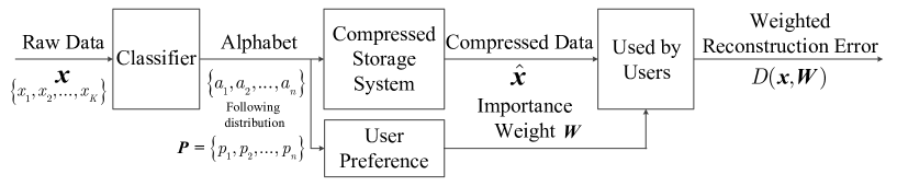
Figure 1: Pictorial representation of the system model.

Consider the situation where the data is stored by its category for easier retrieval, which can make the recommendation system based on it more effective [32]. Since that data classification becomes increasingly convenient and accurate nowadays due to the rapid development of machine learning [34, 35], this paper assumes that the event class can be easily detected and known in storage system. Moreover, assume the data which belongs to the same class has the same importance-weight and occupies the same storage size. Hence, x can be seen as a sequence of $K$ symbols from an alphabet $\{a_{1},a_{2},...,a_{n}\}$ where $a_{i}$ represent event class $i$. In this case, the weighted reconstruction error based on importance is formulated as

$$D({\emph{{x}}},{\emph{{W}}}) =\sum\nolimits_{i=1}^{n}\frac{N(a_{i}|{\emph{{x}}})}{K}W_{i}D_{f}(Sa_{i},S{\hat{a}}_{i})$$ (2)

$$=\sum\nolimits_{i=1}^{n}p_{i}W_{i}D_{f}(Sa_{i},S{\hat{a}}_{i}),$$ (2a)

where $N(a_{i}|{\emph{{x}}})$ is the number of times the $i$-class occurs in the sequence x. Let $p_{i}={N(a_{i}|{\emph{{x}}})}/{K}$ to denote the probability distribution of event class $i$ in data sequence x.

II-B Modeling Distortion between the Raw Data and the Compressed Data

In general, the data storage system is lack of storage space when faced with super-large scale of data. If there is limited storage resources which can be assigned to data, the optimization of storage resource allocation will be indispensable. To frame the problem appropriately, it is imperative to characterize the distortion between the raw data and the compressed data with specified storage size. Usually, there is no universal characterization of this distortion measure, especially in speech coding and image coding [33]. In order to facilitate the analysis and design, this paper will discuss the following special case.

We assume that the data is digital. The description of the raw data $a_{i}$ requires $L_{i}$ bits, and $a_{i}=\sum\nolimits_{j=0}^{L_{i}-1}b_{j}\times r^{j}$ where $r$ is radix ($r>1$). In particular, $L_{i}$ will approach the infinite number if $a_{i}$ is arbitrary real number. In the storage system of this paper, there is only $l_{i}$ bits assigned to it. For convenience, the smaller $L_{i}-l_{i}$ numbers is discarded, and they are random numbers in actual system. Thus, the compressed data is $\hat{a}_{i}=\sum\nolimits_{j=L_{i}-l_{i}}^{L_{i}-1}b_{j}\times r^{j}+\sum\nolimits_{j=0}^{L_{i}-l_{i}-1}b^{*}_{j}\times r^{j}$ where $b^{*}_{j}$ is a random number in $\{0,...,r-1\}$. The absolute error is $|a_{i}-\hat{a}_{i}|$, which meets

$$|a_{i}-\hat{a}_{i}|\leq r^{L_{i}-l_{i}}-1.$$ (3)

When $l_{i}=0$, which means there is no information stored, the absolute error reaches the maximum and it is $|a_{i}-\hat{a}_{i}|=r^{L_{i}}-1$. This paper defines the relative error which is normalized by the maximum absolute error as the distortion measure, which is given by

$$D_{f}(Sa_{i},S{\hat{a}}_{i})=D_{f}(L_{i},l_{i})=\frac{r^{L_{i}-l_{i}}-1}{r^{L_{i}}-1}.$$ (4)

In particular, we obtain $D_{f}(L_{i},L_{i})=0$ and $D_{f}(L_{i},0)=1$. Moreover, it is easy to check that $0\leq D_{f}(L_{i},l_{i})\leq 1$ and $D_{f}(L_{i},l_{i})$ decreases with the increasing of $l_{i}$.

To simplify the comparisons under different conditions , the weighted reconstruction error is also normalized to the RWRE. Then the RWRE is given by

$$D_{r}({\emph{{x}}},{\emph{{W}}})=D_{r}(\emph{{W}},\emph{{L}},\emph{{l}})=\frac{D({\emph{{x}}},{\emph{{W}}})}{\mathop{\max}\limits_{l_{i}}D({\emph{{x}}},{\emph{{W}}})}=\frac{\sum\nolimits_{i=1}^{n}p_{i}W_{i}D_{f}(L_{i},l_{i})}{\sum\nolimits_{i=1}^{n}p_{i}W_{i}}=\frac{\sum\nolimits_{i=1}^{n}p_{i}W_{i}\frac{r^{L_{i}-l_{i}}-1}{r^{L_{i}}-1}}{\sum\nolimits_{i=1}^{n}p_{i}W_{i}},$$ (5)

where $\emph{{L}}=\{L_{1},...,L_{n}\}$ and $\emph{{l}}=\{l_{1},...,l_{n}\}$.

II-C Problem Formulation

II-C1 General Storage System

In fact, the available storage space can then be expressed as $\sum\nolimits_{i=1}^{n}p_{i}l_{i}$. For each given target maximum available storage space constraint $\sum\nolimits_{i=1}^{n}p_{i}l_{i}\leq T$, we shall optimize storage resources allocation strategy of this system by minimizing the RWRE, which can be expressed as

$$\mathcal{P}_{1}:\,\,\mathop{\min}\limits_{l_{i}}\,\,\, D_{r}({\emph{{x}}},{\emph{{W}}})$$ (6)

s.t. $$\sum\limits_{i=1}^{n}p_{i}l_{i}\leq T$$ (6a)

$$0\leq l_{i}\leq L_{i}\,\,\textrm{for}\,\,i=1,2,...,n.$$ (6b)

The storage systems which can be characterized by Problem $\mathcal{P}_{1}$ are referred to as general storage system.

Remark 1.

In fact, this paper focuses on allocating resources by category with taking message importance into account, while the conventional source coding searches the shortest average description length of a random variable.

II-C2 Ideal Storage system

In practice, the storage size of raw data is the same frequently for ease of use. Thus, we focus on the case where the original storage size is the same for simplifying the analysis in this paper, and use $L$ to denote it (i.e., $L_{i}=L$ for $i=1,2,...,n$). As a result, we have

$$\mathop{\min}\limits_{l_{i}}D_{r}({\emph{{x}}},{\emph{{W}}})=\frac{r^{L}\mathop{\min}\limits_{l_{i}}\sum\limits_{i=1}^{n}p_{i}W_{i}{r^{-l_{i}}}}{(r^{L}-1)\sum\limits_{i=1}^{n}p_{i}W_{i}}-\frac{1}{r^{L}-1}.$$ (7)

Thus, the problem $\mathcal{P}_{1}$ can be rewritten as

$$\mathcal{P}_{2}:\,\,\mathop{\min}\limits_{l_{i}}\,\,\, \sum\limits_{i=1}^{n}p_{i}W_{i}r^{-l_{i}}$$ (8)

s.t. $$\sum\limits_{i=1}^{n}p_{i}l_{i}\leq T$$ (8a)

$$0\leq l_{i}\leq L\,\,\textrm{for}\,\,i=1,2,...,n.$$ (8b)

Since we will mainly focus on the characteristics of the solutions in Problem $\mathcal{P}_{2}$ in this paper, we use ideal storage system to represent this model in later sections of this paper.

II-C3 Quantification Storage System

A quantification storage system quantizes and stores the real data acquired from sensors in the real world. The data is usually a real number, which requires infinite number bits to describe it accurately. That is, the original storage size of each class approaches the infinite number, (i.e., $L_{i}=L\to+\infty$ for $i=1,2,...,n$), in this case. As a result, the RWRE can be rewritten as

$$D_{r}({\emph{{x}}},{\emph{{W}}})=\mathop{\lim}\limits_{L\to\infty}\left\{\frac{\sum\limits_{i=1}^{n}p_{i}W_{i}{r^{-l_{i}}}}{(1-r^{-L})\sum\limits_{i=1}^{n}p_{i}W_{i}}-\frac{1}{r^{L}-1}\right\}=\frac{\sum\limits_{i=1}^{n}p_{i}W_{i}{r^{-l_{i}}}}{\sum\limits_{i=1}^{n}p_{i}W_{i}}.$$ (9)

Therefore, the problem $\mathcal{P}_{1}$ in this case is reduced to

$$\mathcal{P}_{3}:\,\,\mathop{\min}\limits_{l_{i}}\,\,\, \sum\limits_{i=1}^{n}p_{i}W_{i}r^{-l_{i}}$$ (10)

s.t. $$\sum\limits_{i=1}^{n}p_{i}l_{i}\leq T$$ (10a)

$$l_{i}\geq 0\,\,\textrm{for}\,\,i=1,2,...,n.$$ (10b)

III Optimal Allocation Strategy with Limited Storage Space

In this section, we shall first solve the problem $\mathcal{P}_{1}$ and give the solutions. In fact, the solutions provide the optimal storage space allocation strategy for digital data on the best effort in minimizing the RWRE when the total available storage size is limited. Then, the problem $\mathcal{P}_{2}$ will be solved, whose solution characterizes the optimal storage space allocation strategy with the same original storage size. Moreover, we shall also discuss the solution in the case where the original storage size of each class approaches the infinite number by studying the problem $\mathcal{P}_{3}$.

III-A Optimal Allocation Strategy in General Storage System

Theorem 1.

For a storage system with probability distribution $(p_{1},p_{2},...,p_{n})$, $L_{i}$ is the storage size of the raw data of the class $i$ for $i=1,2,...,n$. For a given maximum available storage space $T$ ($0\leq T\leq\sum\nolimits_{i=1}^{n}p_{i}L_{i}$), when the radix is $r$ ($r>1$), the solution of Problem $\mathcal{P}_{1}$ is given by

$$l_{i}= \left\{\begin{aligned} &\quad\quad\quad\quad 0\quad\quad\quad\quad\quad\quad\quad\quad\quad\quad\quad\quad\quad\,\,\,\,\,\,\,\textit{if}\,\,l_{i}<0,\\ &\frac{\ln(\ln r)+\ln W_{i}-\ln(1-r^{-L_{i}})-\ln\lambda^{*}}{\ln r}\quad\quad\textit{if}\,\,0\leq l_{i}\leq L_{i},\\ &\quad\quad\quad\quad L_{i}\quad\quad\quad\quad\quad\quad\quad\quad\quad\quad\quad\quad\quad\,\,\,\,\,\textit{if}\,\,l_{i}>L_{i},\end{aligned}\right.$$ (11)

where $\lambda^{*}$ is chosen so that $\sum\nolimits_{i=1}^{n}p_{i}l_{i}=T$.

Proof.

By means of Lagrange multipliers and Karush-Kuhn-Tucher conditions, when ignoring the constant $\sum\nolimits_{i=1}^{n}p_{i}W_{i}$, we set up the functional

$${\nabla_{l}}\left\{{\sum\limits_{i=1}^{n}p_{i}W_{i}\frac{r^{L_{i}-l_{i}}-1}{r^{L_{i}}-1}}+\lambda^{*}(\sum\limits_{i=1}^{n}p_{i}l_{i}-T)+\mu_{1}(l_{1}-L_{1})+...+\mu_{n}(l_{n}-L_{n})\right\}=0$$ (12)

$$\sum\limits_{i=1}^{n}p_{i}l_{i}-T=0$$ (12a)

$$\mu_{i}(l_{i}-L_{i})=0\,\,\textrm{for}\,\,i=1,2,...,n$$ (12b)

$$l_{i}-L_{i}\leq 0\,\,\textrm{for}\,\,i=1,2,...,n$$ (12c)

$$\mu_{i}\geq 0\,\,\textrm{for}\,\,i=1,2,...,n$$ (12d)

$$l_{i}\geq 0\,\,\textrm{for}\,\,i=1,2,...,n$$ (12e)

Hence, we obtain

$$l_{i}=\frac{\ln p_{i}+\ln(\ln r)+\ln W_{i}-\ln(1-r^{-L_{i}})-\ln(\lambda^{*}p_{i}+\mu_{i})}{\ln r}.$$ (13)

First, it is easy to check that Equation (12b)-(12d) hold when $\mu_{i}=0$ and $l_{i}\leq L_{i}$. Hence, we have

$$l_{i}=\frac{\ln(\ln r)+\ln W_{i}-\ln(1-r^{-L_{i}})-\ln\lambda^{*}}{\ln r}.$$ (14)

Second, if $l_{i}$ in Equation (13) is larger than $L_{i}$, we will have $\mu_{i}>0$ and $l_{i}=L_{i}$ due to Equation (12b)-(12d).

Third, if $l_{i}<0$, we will let $l_{i}=0$ according to Equation (12e).

Moreover, $\lambda^{*}$ is chosen so that $\sum\nolimits_{i=1}^{n}p_{i}l_{i}=T$ due to Equation (12a).

Therefore, based on the discussion above, we get Equation (11) in order to ensure $0\leq l_{i}\leq L_{i}$. ∎

Remark 2.

Let ${\tilde{N}}$ be the number of $l_{i}$ which meets $0\leq l_{i}\leq L_{i}$ and $\{I_{j},j=1,2,...,\tilde{N}\}$ is part of the sequence of $\{1,2,...,N\}$ which satisfies $0\leq{\ln(\ln r)+\ln W_{I_{j}}-\ln(1-r^{-L_{I_{j}}})-\ln\lambda^{*}}\leq L_{I_{j}}{\ln r}$. Furthermore, $\{T_{j},j=1,2,...,\tilde{N}_{L}\}$ is used to denote the part of the sequence of $\{1,2,...,N\}$ which satisfies ${\ln(\ln r)+\ln W_{T_{j}}-\ln(1-r^{-L_{T_{j}}})-\ln\lambda^{*}}>L_{T_{j}}{\ln r}$.

Substituting Equation (11) in the constraint $\sum\nolimits_{i=1}^{n}p_{i}l_{i}=T$, we have

$$\ln\lambda^{*}=\ln\ln r+\frac{\sum\nolimits_{j=1}^{\tilde{N}}p_{I_{j}}\ln W_{I_{j}}-\sum\nolimits_{j=1}^{\tilde{N}}p_{I_{j}}\ln(1-r^{-L_{I_{j}}})-\ln r(T-\sum\nolimits_{j=1}^{\tilde{N}_{L}}p_{T_{j}}L_{T_{j}})}{\sum\nolimits_{j=1}^{\tilde{N}}p_{I_{j}}}.$$ (15)

Hence, for $0\leq l_{i}\leq L$, we obtain

$$l_{i}=\frac{T-\sum\nolimits_{j=1}^{\tilde{N}_{L}}p_{T_{j}}L_{T_{j}}}{\sum\nolimits_{j=1}^{\tilde{N}}p_{I_{j}}}+\frac{\ln W_{i}}{\ln r}-\frac{{\sum\nolimits_{j=1}^{\tilde{N}}p_{I_{j}}\ln W_{I_{j}}}}{\ln r{\sum\nolimits_{j=1}^{\tilde{N}}p_{I_{j}}}}+\frac{{\sum\nolimits_{j=1}^{\tilde{N}}p_{I_{j}}\ln(1-r^{-L_{I_{j}}})}}{\ln r{\sum\nolimits_{j=1}^{\tilde{N}}p_{I_{j}}}}.$$ (16)

In fact, $T$, $p_{i}$, $r$, $L_{i}$ are usually constraints for a given recommendation system, and therefore $l_{i}$ is only determined by the second and the third items on the right side of Equation (16), which means the storage size depends on the message importance and the probability distribution of class for given available storage size.

Remark 3.

Since the actual compressed storage size $l^{*}_{i}$ must be integer, the actual storage size allocation strategy is

$$l^{*}_{i}=\min\left({\left\lfloor\frac{T-\sum\nolimits_{j=1}^{\tilde{N}_{L}}p_{T_{j}}L_{T_{j}}}{\sum\nolimits_{j=1}^{\tilde{N}}p_{I_{j}}}+\frac{\ln W_{i}}{\ln r}-\frac{{\sum\nolimits_{j=1}^{\tilde{N}}p_{I_{j}}\ln W_{I_{j}}}}{\ln r{\sum\nolimits_{j=1}^{\tilde{N}}p_{I_{j}}}}+\frac{{\sum\nolimits_{j=1}^{\tilde{N}}p_{I_{j}}\ln(1-r^{-L_{I_{j}}})}}{\ln r{\sum\nolimits_{j=1}^{\tilde{N}}p_{I_{j}}}}\right\rfloor}^{+},L\right),$$ (17)

where $(x)^{+}$ is equal to $x$ when $x\geq 0$, and it is zero when $x<0$. In addition, $\lfloor x\rfloor$ is the largest integer smaller than or equal to $x$.

III-B Optimal Allocation Strategy in Ideal Storage System

Then, we pay attention to the case where the original storage size is the same for simplifying the analysis. Based on Theorem 1, we get the following corollary in ideal storage system.

Corollary 1.

For a storage system with probability distribution $(p_{1},p_{2},...,p_{n})$, the original storage size of each class is the same, which is given by $L_{i}=L$ for $i=1,2,...,n$. For a given maximum available storage space $T$ ($0\leq T\leq L$), when the radix is $r$ ($r>1$), the solution of Problem $\mathcal{P}_{2}$ is given by

$$l_{i}= \left\{\begin{aligned} &\quad\quad 0\quad\quad\quad\quad\quad\quad\quad\,\,\,\,\quad\,\,\textrm{if}\,\,l_{i}<0,\\ &\frac{\ln(\ln r)+\ln W_{i}-\ln\lambda}{\ln r}\quad\,\,\,\,\textrm{if}\,\,0\leq l_{i}\leq L,\\ &\quad\quad L\quad\quad\quad\quad\quad\quad\quad\,\,\,\,\,\quad\textrm{if}\,\,l_{i}>L,\end{aligned}\right.$$ (18)

where $\lambda$ is chosen so that $\sum\nolimits_{i=1}^{n}p_{i}l_{i}=T$.

Proof.

Let $\lambda=\lambda^{*}(1-r^{-L})$ and $L_{i}=L$ for $i=1,2,...,n$. Substituting them in Equation (11), we find that $l_{i}$ in this case can be rewritten as Equation (18). ∎

Substituting Equation (18) in the constraint $\sum\nolimits_{i=1}^{n}p_{i}l_{i}=T$, we obtain

$$\ln\lambda=\ln\ln r+\frac{\sum\nolimits_{j=1}^{\tilde{N}}p_{I_{j}}\ln W_{I_{j}}-\ln r(T-T_{N_{L}})}{\sum\nolimits_{j=1}^{\tilde{N}}p_{I_{j}}},$$ (19)

where $\tilde{N}$, $\tilde{N}_{L}$, $I_{j}$, $T_{j}$ is still given by Remark 2 with letting $\lambda^{*}=\lambda^{*}(1-r^{-L})$. In addition, $T_{N_{L}}=\sum\nolimits_{j=1}^{\tilde{N}_{L}}p_{T_{j}}L$. Hence, for $0\leq l_{i}\leq L$, we obtain

$$l_{i}=\frac{T-T_{N_{L}}}{\sum\nolimits_{j=1}^{\tilde{N}}p_{I_{j}}}+\frac{\ln W_{i}}{\ln r}-\frac{{\sum\nolimits_{j=1}^{\tilde{N}}p_{I_{j}}\ln W_{I_{j}}}}{\ln r{\sum\nolimits_{j=1}^{\tilde{N}}p_{I_{j}}}}.$$ (20)

Remark 4.

Since the actual compressed storage size $l^{*}_{i}$ must be integer, the actual storage size allocation strategy is

$$l^{*}_{i}=\min\left({\left\lfloor\frac{T-T_{N_{L}}}{\sum\nolimits_{j=1}^{\tilde{N}}p_{I_{j}}}+\frac{\ln W_{i}}{\ln r}-\frac{{\sum\nolimits_{j=1}^{\tilde{N}}p_{I_{j}}\ln W_{I_{j}}}}{\ln r{\sum\nolimits_{j=1}^{\tilde{N}}p_{I_{j}}}}\right\rfloor}^{+},L\right).$$ (21)

Remark 5.

When ${\tilde{N}}=n$, $0\leq l_{i}\leq L$ always holds for $1\leq i\leq n$, and the actual storage size is given by

$$l^{*}_{i}=\left\lfloor T+\frac{\ln W_{i}-{\sum\nolimits_{i=1}^{n}p_{i}\ln W_{i}}}{\ln r}\right\rfloor.$$ (22)

In order to illustrate the geometric interpretation of this algorithm, we might as well take

$$\beta=\frac{\ln\ln r-\ln\lambda}{\ln r},$$ (23)

and the optimal storage size can be simplified to

$$l_{i}= \left\{\begin{aligned} &\quad\quad 0,\quad\quad\quad\quad\quad\quad\quad\,\,\,\,\textrm{if}\,\,\beta-\frac{\ln(1/W_{i})}{\ln r}<0.\\ &\beta-\frac{\ln(1/W_{i})}{\ln r}\quad\quad\,\,\,\quad\quad\textrm{if}\,\,0\leq\beta-\frac{\ln(1/W_{i})}{\ln r}\leq L.\\ &\quad\quad L,\quad\quad\quad\quad\quad\quad\quad\,\,\,\,\textrm{if}\,\,\beta-\frac{\ln(1/W_{i})}{\ln r}>L.\end{aligned}\right.$$ (24)

The monotonicity of optimal storage size with respect to importance weight is discussed in the following theorem.

Theorem 2.

Let $(p_{1},p_{2},...,p_{n})$ be a probability distribution and ${{\textrm{W}}}={W_{1},...,W_{n}}$ be importance weights. $L$ and $r$ are fixed positive integers ($r>1$). The solution of Problem $\mathcal{P}_{2}$ meets: $l_{i}\geq l_{j}$ if $W_{i}>W_{j}$ for $\forall i,j\in\{1,2,...,n\}$.

Proof.

Refer to the Appendix A-A. ∎

This gives rise to a kind of restrictive water-filling, which is presented in Figure 2. Choose a constant $\beta$ so that $\sum\nolimits_{i=1}^{n}p_{i}l_{i}=T$. The storage size depends on the difference between $\beta$ and $\frac{\ln(1/W_{i})}{\ln r}$. In Figure 2, we obtain that $\beta$ characterizes the height of water surface, and $\frac{\ln(1/W_{i})}{\ln r}$ determines the bottom of the pool. Actually, no storage space is assigned to the data with this difference less than zero. When the difference is in the interval $[0,L]$, this difference is exactly the storage size. Furthermore, the storage size will be truncated to $L$ bits if the difference is larger than $L$. Compared with the conventional water-filling, the lowest height of the bottom of the pool is constricted in this restrictive water-filling.

Remark 6.

The restrictive water-filling in Figure 2 is summarized as follows.

• For the data with extremely small message importance, $\frac{\ln(1/W_{i})}{\ln r}$ is so large that the bottom of the pool is above the water surface. Thus, the storage size of this kind of data is zero.

• For the data with small message importance, $\frac{\ln(1/W_{i})}{\ln r}$ is large, and therefore the bottom of the pool is high. Thus, the storage size of this kind of data is small.

• For the data with large message importance, $\frac{\ln(1/W_{i})}{\ln r}$ is small, and therefore the bottom of the pool is low. Thus, the storage size of this kind of data is large.

• For the data with extremely large message importance, $\frac{\ln(1/W_{i})}{\ln r}$ is so small that the bottom of the pool is constricted in order to truncate the storage size to $L$.

Thus, this optimal storage space allocation strategy is a high efficiency adaptive storage allocation algorithm for the fact that it can make rational use of all the storage space according to message importance to minimize the RWRE.

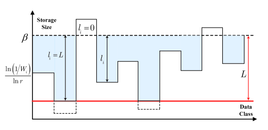
Figure 2: Restrictive water-filling for optimal storage size.

This solution can be gotten by means of recursive algorithm in practice, which is shown in Algorithm 1, where we define an auxiliary function as

$$f(i,\emph{{W}},\emph{{p}},L,T,r,K_{\min},K_{\max})=\frac{T}{\sum\nolimits_{j=K_{\min}}^{K_{\max}}p_{j}}+\frac{\ln W_{i}}{\ln r}-\frac{{\sum\nolimits_{j=K_{\min}}^{K_{\max}}p_{j}\ln W_{j}}}{\ln r{\sum\nolimits_{j=K_{\min}}^{K_{\max}}p_{j}}}.$$ (25)

Algorithm 1 Storage Space Allocation Algorithm

0:    The message importance, $\emph{{W}}=\{W_{i},i=1,2,...,n\}$ (Sort it to satisfy $W_{1}\geq W_{2}\geq...\geq W_{n}$) The probability distribution of source, $\emph{{P}}=\{p_{i},i=1,2,...,n\}$ The original storage size, $L$ The maximum available storage space, $T$ The radix, $r$ The auxiliary variables, $K_{\min},K_{\max}$ (Let $K_{\min}=1,K_{\max}=n$ as the original values)

0:     The compressed code length, $\emph{{l}}=\{l_{i},i=K_{\min},...,K_{\max}\}$ Denote the following algorithm as $\{l_{K_{\min}},...,l_{K_{\max}}\}=\phi(\emph{{W}},\emph{{P}},L,T,r,K_{\min},K_{\max})$

1:  ${l_{i}}^{\prime}\leftarrow f(i,\emph{{W}},\emph{{P}},L,T,r,K_{\min},K_{\max})$ for $i=K_{\min},...,K_{\max}$      $\vartriangleright$ See Equation (25)

2:  if $\forall t\in\{K_{\min},...,K_{\max}\}$ such that $0\leq l_{t}^{\prime}\leq L$ and $\sum\nolimits_{i=K_{\min}}^{K_{\max}}p_{i}l_{i}^{\prime}=T$

3:  ${l_{i}}\leftarrow{l_{i}}^{\prime}$ for $i=K_{\min},...,K_{\max}$

4:  else  if $K_{\max}>K_{\min}$

5:     ${l_{i}}^{(1)}\leftarrow L$ for $i=1,..,K_{\min}-1$

6:     ${l_{i}}^{(1)}\leftarrow 0$ for $i=K_{\max},...,n$

7:     ${l_{i}}^{(1)}\leftarrow\phi(\emph{{W}},\emph{{P}},L,T,r,K_{\min},K_{\max}-1)$ for $i=K_{\min},...,K_{\max}-1$

8:     $\epsilon^{(1)}=D_{r}(\emph{{W}},L,\emph{{l}}^{(1)})$                  $\vartriangleright$ See Equation (5)

9:     ${l_{i}}^{(2)}\leftarrow L$ for $i=1,..,K_{\min}$

10:     ${l_{i}}^{(2)}\leftarrow 0$ for $i=K_{\max}+1,...,n$

11:     $T^{\prime}\leftarrow T-p_{K_{\min}}L$

12:     ${l_{i}}^{(2)}\leftarrow\phi(\emph{{W}},\emph{{P}},L,T^{\prime},r,K_{\min}+1,K_{\max})$ for $i=K_{\min}+1,...,K_{\max}$

13:     $\epsilon^{(2)}=D_{r}(\emph{{W}},L,\emph{{l}}^{(2)})$                  $\vartriangleright$ See Equation (5)

14:       if $\epsilon^{(1)}\geq\epsilon^{(2)}$

15:         ${l_{i}}\leftarrow{l_{i}}^{(1)}$ for $i=1,2,...,n$

16:       else

17:         ${l_{i}}\leftarrow{l_{i}}^{(2)}$ for $i=1,2,...,n$

18:       end

19:     else

20:     ${l_{i}}\leftarrow L$ for $i=1,..,K_{\min}-1$

21:     ${l_{i}}\leftarrow 0$ for $i=K_{\min}+1,...,n$

22:     ${l_{K_{\min}}}\leftarrow(T-\sum\nolimits_{i=1}^{K_{\min}-1}p_{i}L)/p_{K_{\min}}$

23:     end

24:  end

25:  return  $l_{i}$ for $i=K_{\min},...,K_{\max}$

III-C Optimal Allocation Strategy in Quantification Storage System

Corollary 2.

For a given maximum available storage space $T$ ($T\geq 0$), when probability distribution is $(p_{1},p_{2},...,p_{n})$ and the radix is $r$ ($r>1$), the solution of Problem $\mathcal{P}_{3}$ is given by

$$l_{i}=\left(\frac{\ln(\ln r)+\ln W_{i}-\ln\lambda}{\ln r}\right)^{+},$$ (26)

where $\lambda$ is chosen so that $\sum\nolimits_{i=1}^{n}p_{i}l_{i}=T$.

Proof.

Let $L\to\infty$ in Corollary 1, the solutions in Equation (18) can be simplified to Equation (26). ∎

In fact, the optimal storage space allocation strategy in this case can be seen as a kind of water-filling, which gets rid of the constraint on the lowest height of the bottom of the pool.

IV Property of Optimal Storage Strategy Based on Message Importance Measure

Considering that the ideal storage system can capture most of characteristics of the lossy compression storage model in this paper, we focus on the property of optimal storage strategy in it in this section for ease of analyzing. Specifically, we ignore rounding and adopt $l_{i}$ in Equation (18) as the optimal storage size of the $i$-th class in this section. Moreover, we focus on a special kind of the importance weight. Namely, MIM is adopted as the importance weight in this paper, for the fact that it can effectively measure the cost of the error in data reconstruction in the small-probability event scenarios [21, 30].

IV-A Normalized MIM

In order to facilitate comparison under different parameters, the normalized MIM is used and we can write

$$W_{i}=\frac{e^{\varpi(1-p_{i})}}{\sum\nolimits_{j=1}^{n}e^{\varpi(1-p_{j})}},$$ (27)

where $\varpi$ is the importance coefficient.

Actually, it is easy to check that $0\leq W_{i}\leq 1$ for $i=1,2,...,n$. Moreover, it is obvious that the sum of those in all event classes is one.

IV-A1 Positive Importance Coefficient

For positive importance coefficient (i.e., $\varpi>0$), let $\alpha_{1}=\arg\mathop{\min}\limits_{i}p_{i}$ and assume $p_{\alpha_{1}}<p_{i}$ for $i\neq\alpha_{1}$. The derivation of it with respect to the importance coefficient is

$$\frac{\partial W_{\alpha_{1}}}{\partial\varpi}=\frac{\sum\nolimits_{j=1}^{n}(p_{j}-p_{\alpha_{1}})e^{\varpi(2-p_{\alpha_{1}}-p_{j})}}{{\left(\sum\nolimits_{j=1}^{n}e^{\varpi(1-p_{j})}\right)}^{2}}\geq 0.$$ (28)

Therefore, $W_{\alpha_{1}}$ increases as $\varpi$ increases. In particular, as $\varpi$ approaches positive infinity, we have

$$\mathop{\lim}\limits_{\varpi\to+\infty}W_{\alpha_{1}}= \mathop{\lim}\limits_{\varpi\to+\infty}\frac{e^{\varpi(1-p_{\alpha_{1}})}}{\sum\nolimits_{j=1}^{n}e^{\varpi(1-p_{j})}}$$ (29)

$$= \mathop{\lim}\limits_{\varpi\to+\infty}\frac{e^{\varpi(1-p_{\alpha_{1}})}}{e^{\varpi(1-p_{\alpha_{1}})}+\sum\nolimits_{j\neq\alpha_{1}}e^{\varpi(1-p_{j})}}$$ (29a)

$$= \mathop{\lim}\limits_{\varpi\to+\infty}\frac{1}{1+\sum\nolimits_{j\neq\alpha_{1}}e^{\varpi(p_{\alpha_{1}}-p_{j})}}$$ (29b)

$$= 1.$$ (29c)

Obviously, $\mathop{\lim}\limits_{\varpi\to+\infty}W_{i}=0$ for $i\neq\alpha_{1}$.

Remark 7.

As $\varpi$ approaches positive infinity, the importance weight with the smallest probability is one and others are all zero, which means only a fraction of data almost owns almost all of the critical information that users care about in the viewpoint of this message importance.

IV-A2 Negative Importance Coefficient

When importance coefficient is negative (i.e., $\varpi<0$), let $\alpha_{2}=\arg\mathop{\max}\limits_{i}p_{i}$ and assume $p_{\alpha_{2}}>p_{i}$ for $i\neq\alpha_{2}$. The derivation of it with respect to the importance coefficient is

$$\frac{\partial W_{\alpha_{2}}}{\partial\varpi}=\frac{\sum\nolimits_{j=1}^{n}(p_{j}-p_{\alpha_{2}})e^{\varpi(2-p_{\alpha_{2}}-p_{j})}}{{\left(\sum\nolimits_{j=1}^{n}e^{\varpi(1-p_{j})}\right)}^{2}}\leq 0.$$ (30)

Therefore, $W_{\alpha_{1}}$ decreases as $\varpi$ increases. In particular, as $\varpi$ approaches negative infinity, we have

$$\mathop{\lim}\limits_{\varpi\to-\infty}W_{\alpha_{2}}= \mathop{\lim}\limits_{\varpi\to-\infty}\frac{e^{\varpi(1-p_{\alpha_{2}})}}{\sum\nolimits_{j=1}^{n}e^{\varpi(1-p_{j})}}$$ (31)

$$= \mathop{\lim}\limits_{\varpi\to-\infty}\frac{e^{\varpi(1-p_{\alpha_{2}})}}{e^{\varpi(1-p_{\alpha_{2}})}+\sum\nolimits_{j\neq\alpha_{2}}e^{\varpi(1-p_{j})}}$$ (31a)

$$= \mathop{\lim}\limits_{\varpi\to-\infty}\frac{1}{1+\sum\nolimits_{j\neq\alpha_{2}}e^{\varpi(p_{\alpha_{2}}-p_{j})}}$$ (31b)

$$= 1.$$ (31c)

Obviously, $\mathop{\lim}\limits_{\varpi\to-\infty}W_{i}=0$ for $i\neq\alpha_{2}$.

Remark 8.

As $\varpi$ approaches negative infinity, the importance weight with the biggest probability is one and others are all zero. If the biggest probability is not too big, the majority of message importance can also be included in not too much data.

IV-B Optimal Storage Size for Each Class

Assume ${\tilde{N}}=n$ and ignore rounding, due to Equation (22), we obtain

$$l_{i}= T+\frac{\ln\frac{e^{\varpi(1-p_{i})}}{\sum\nolimits_{j=1}^{n}e^{\varpi(1-p_{j})}}-\sum\limits_{i=1}^{n}{p_{i}\ln\frac{e^{\varpi(1-p_{i})}}{\sum\nolimits_{j=1}^{n}e^{\varpi(1-p_{j})}}}}{\ln r}$$ (32)

$$= T+\frac{\varpi}{\ln r}({\gamma_{p}}-p_{i}),$$ (32a)

where $\gamma_{p}$ is an auxiliary variable and it is given by

$$\gamma_{p}=\sum\limits_{i=1}^{n}p_{i}^{2}.$$ (33)

In fact, its natural logarithm is the minus Rényi entropy of order two, i.e., $\gamma_{p}=e^{-H_{2}(\emph{{P}})}$ where $H_{2}(\emph{{P}})$ is the Rényi entropy $H_{\alpha}(\cdot)$ when $\alpha=2$ [36]. Furthermore, we have the following lemma on $\gamma_{p}$.

Lemma 1.

Let $(p_{1},p_{2},...,p_{n})$ be a probability distribution, then we have

$$\frac{1}{n} \leq\gamma_{p}\leq 1,$$ (34)

$$-\frac{1}{4} \leq\gamma_{p}-p_{i}\leq 1.$$ (34a)

Proof.

Refer to the Appendix A-B. ∎

Thus, we find $l_{i}>T$ if $(1/n-p_{i})\varpi>0$. Besides, we obtain $l_{i}=T$ when $p_{i}=\gamma_{p}$.

Theorem 3.

Let $(p_{1},p_{2},...,p_{n})$ be a probability distribution and $W_{i}={e^{\varpi(1-p_{i})}}/{\sum\nolimits_{j=1}^{n}e^{\varpi(1-p_{j})}}$ be importance weight. The optimal storage size in ideal storage system has the following properties:

1. $l_{i}\geq l_{j}$ if $p_{i}<p_{j}$ for $\forall i,j\in\{1,2,...,n\}$ when $\varpi>0$;

2. $l_{i}\leq l_{j}$ if $p_{i}<p_{j}$ for $\forall i,j\in\{1,2,...,n\}$ when $\varpi<0$.

Proof.

Refer to the Appendix A-C. ∎

Remark 9.

Due to [30], the data with smaller probability usually possesses larger importance when $\varpi>0$, while the data with larger probability usually possesses larger importance when $\varpi<0$. Therefore, this optimal allocation strategy makes rational use of all the storage space by providing more storage size for paramount data and less storage size for insignificance data. It agrees with the intuitive idea, which is that users generally are more concerned about the data that they need rather than the whole data itself.

Lemma 2.

Let $(p_{1},p_{2},...,p_{n})$ be a probability distribution and $r$ be radix. $L$ and $T$ are integers, and $T<L$. If $\varpi$ meets $0\leq T+{\varpi(\gamma_{p}-p_{i})}/{\ln r}\leq L$, then we have ${\tilde{N}}=n$.

Proof.

According to Equation (32a) and constraint $0\leq T+{\varpi(\gamma_{p}-p_{i})}/{\ln r}\leq L$, we obtain $0\leq l_{i}\leq L$ for $\forall i\in\{1,2,...,n\}$. In this case, ${\tilde{N}}=n$. ∎

In fact, when $\varpi\geq 0$, due to Equation (32a) and Lemma 1, we obtain

$$0\leq T-\frac{\varpi}{4\ln r}\leq T+\frac{\varpi(\gamma_{p}-p_{i})}{\ln r} \leq T+\frac{\varpi}{\ln r}\leq L.$$ (35)

Similarly, when $\varpi<0$, we have

$$0\leq T+\frac{\varpi}{\ln r}\leq T+\frac{\varpi(\gamma_{p}-p_{i})}{\ln r} \leq T-\frac{\varpi}{4\ln r}\leq L.$$ (36)

According to Equation (35) and Equation (36), we find ${\tilde{N}}=n$ always holds If $\max(4\ln r(T-L),-T/\ln r)\leq\varpi\leq\min(4T\ln r,\ln r(L-T))$.

IV-C Relative Weighted Reconstruction Error

For convenience, $D({\emph{{x}}},\varpi)$ is used to denote $D({\emph{{x}}},{\emph{{W}}})$. Due to Equation (7), we have

$$D_{r}({\emph{{x}}},\varpi)=\frac{1}{r^{L}-1}\left({\frac{\sum\nolimits_{i=1}^{n}p_{i}e^{\varpi(1-p_{i})}r^{L-l_{i}}}{\sum\nolimits_{i=1}^{n}p_{i}e^{\varpi(1-p_{i})}}-1}\right).$$ (37)

If $T$ is zero, then we will have $l_{i}=0$ for $i=1,2,...,n$. In this case, $D_{r}({\emph{{x}}},\varpi)=1$. On the contrary, $D_{r}({\emph{{x}}},\varpi)=0$ when $l_{i}=L$ for $i=1,2,...,n$.

Theorem 4.

$D_{r}({{\textbf{x}}},\varpi)$ has the following properties:

1. $D_{r}({{\textbf{x}}},\varpi)$ is monotonically decreasing with $\varpi$ in $(0,+\infty)$;

2. $D_{r}({{\textbf{x}}},\varpi)$ is monotonically increasing with $\varpi$ in $(-\infty,0)$;

3. $D_{r}({{\textbf{x}}},\varpi)\leq D_{r}({{\textbf{x}}},0)=(r^{L-T}-1)/(r^{L}-1)$.

Proof.

Refer to the Appendix A-D. ∎

Remark 10.

As shown in Remark 7 and Remark 8, the overwhelming majority of important information will gather in a fraction of data as the importance coefficient increases to negative/positive infinity. Therefore, we can heavily reduce the storage space with extremely small of RWRE with the increasing of the absolute value of importance coefficient. In fact, this special characteristic of weight reflects the effect of users’ preference. That is, it is beneficial for data compression that the data that users care about is highly clustered. Moreover, when $\varpi=0$, all the importance weight is the same, which leads to the incompressibility for the fact that there is no special characteristic of weight for users to make rational use of storage space.

In the following part of this section, we will discuss the case where $0\leq T+{\varpi(\gamma_{p}-p_{i})}/{\ln r}\leq L$, which means all $l_{i}$ can be given by Equation (32a) and $n=\tilde{N}$ due to Lemma 2. In this case, substituting Equation (32a) in Equation (7), the RWRE is

$$D_{r}({\emph{{x}}},\varpi)=\frac{e^{\varpi(1-\gamma_{p})}r^{\Delta}}{(r^{L}-1)\sum\nolimits_{i=1}^{n}{p_{i}e^{\varpi(1-p_{i})}}}-\frac{1}{r^{L}-1},$$ (38)

where $\Delta=L-T$, which characterizes the actual compressed storage space.

Since that $0\leq T+{\varpi(\gamma_{p}-p_{i})}/{\ln r}\leq L$, we have

$$\frac{\varpi(\gamma_{p}-p_{\alpha_{1}})}{\ln r}\leq L-T\leq L-\frac{\varpi(p_{\alpha_{2}}-\gamma_{p})}{\ln r}$$ (39)

Hence,

$$\delta_{1}=\frac{e^{\varpi(1-p_{\alpha_{1}})}}{(r^{L}-1)\sum\nolimits_{i=1}^{n}{p_{i}e^{\varpi(1-p_{i})}}}-\frac{1}{r^{L}-1}\leq D_{r}({\emph{{x}}},\varpi)\leq\frac{e^{\varpi(1-p_{\alpha_{2}})}r^{L}}{(r^{L}-1)\sum\nolimits_{i=1}^{n}{p_{i}e^{\varpi(1-p_{i})}}}-\frac{1}{r^{L}-1}=\delta_{2}.$$ (40)

Theorem 5.

For a given storage system with the probability distribution of data sequence ${\textbf{P}}=(p_{1},p_{2},...,p_{n})$, let $L$, $r$ be fixed positive integers ($r>1$), and $\varpi$ meets $0\leq T+{\varpi(\gamma_{p}-p_{i})}/{\ln r}\leq L$ for $i=1,2,...,n$. For giving upper bound of the RWRE $\delta$ ($\delta_{1}\leq\delta\leq\delta_{2}$ where $\delta_{1}$ and $\delta_{1}$ is defined in Equation (40)), the maximum available compressed storage size $\Delta^{*}(\delta)$ is given by

$$\Delta^{*}(\delta) =\frac{\ln\left(1+\delta(r^{L}-1)\right)+L(\varpi,{\textbf{P}})-\varpi+\varpi\gamma_{p}}{\ln r}$$ (41)

$$\geq\frac{\ln\left(1+\delta(r^{L}-1)\right)}{\ln r},$$ (41a)

where $L(\varpi,{\textbf{P}})=\ln\sum\nolimits_{i=1}^{n}{p_{i}e^{\varpi(1-p_{i})}}$, and the equality of (41a) holds if the probability distribution of data sequence is uniform distribution or the importance coefficient is zero.

Proof.

It is easy to check that ${\tilde{N}}=n$ according to Lemma 2 for the fact that $0\leq T+{\varpi(\gamma_{p}-p_{i})}/{\ln r}\leq L$. Let $D({\emph{{x}}},\varpi)\leq\delta$. By means of Equation (38), we solve this inequality and obtain

$$\Delta\leq\frac{\ln\left(1+\delta(r^{L}-1)\right)+L(\varpi,\emph{{p}})-\varpi+\varpi\gamma_{p}}{\ln r}=\Delta^{*}(\delta),$$ (42)

where $L(\varpi,\emph{{p}})=\ln\sum\nolimits_{i=1}^{n}{p_{i}e^{\varpi(1-p_{i})}}$. Then we have the following inequality:

$$\Delta^{*}(\delta)\overset{(a)}{\geq}\frac{\ln\left(1+\delta(r^{L}-1)\right)+\ln{e^{\sum\nolimits_{i=1}^{n}p_{i}\varpi(1-p_{i})}}-\varpi+\varpi\gamma_{p}}{\ln r}=\frac{\ln\left(1+\delta(r^{L}-1)\right)}{\ln r},$$

where $(a)$ follows from Jensen’s inequality. Since the exponential function is strictly convex, the equality holds only if $\varpi(1-p_{i})$ is constant everywhere, which means $(p_{1},p_{2},...,p_{n})$ is uniform distribution or importance coefficient $\varpi$ is zero. ∎

Remark 11.

In conventional source coding, the encoding length depends on the entropy of sequence, and a sequence is incompressible if its probability distribution is uniform distribution [33]. In Theorem 5, the uniform distribution is also worst case, since the system achieves the minimum compressed storage size. Although the focus is different, they both show that the uniform distribution is detrimental for compression.

Furthermore, it is also noted that

$$\Delta^{*}(\delta)\leq\Delta^{*}(\delta_{2})=L+\frac{\varpi(\gamma_{p}-p_{\alpha_{2}})}{\ln r}\leq L,$$ (43)

for the fact that $\gamma_{p}\leq p_{\alpha_{2}}$. In order to make $\Delta^{*}(\delta_{2})$ approaches $L$, $\gamma_{p}-p_{\alpha_{2}}$ should be as close to zero as possible in the range which $0\leq T+{\varpi(\gamma_{p}-p_{i})}/{\ln r}\leq L$ for $i=1,2,...,n$ holds.

When the importance coefficient is constant, for two probability distributions P and Q, if $L(\varpi,\emph{{P}})+\varpi\gamma_{p}>L(\varpi,\emph{{Q}})+\varpi\gamma_{q}$, then we will obtain $\Delta^{*}$ in P is larger than that in Q. In fact, $L(\varpi,\emph{{p}})$ is defined as MIM in [29], and $\gamma_{p}=e^{-H_{2}(\emph{{P}})}$ [36]. Thus, the maximum available compressed storage size is under the control of MIM and Rényi entropy of order two. For typical small-probability event scenarios where there is a exceedingly small probability, the MIM is usually large, and $\gamma_{p}$ is also not small simultaneously with big probability. Therefore, $\Delta^{*}(\delta)$ is usually large in this case. As a result, much more compressed storage space can be gotten in typical small-probability event scenarios while compared to that in uniform probability distribution. Namely, the data can compressed by means of the characteristic of the typical small-probability events, which may help to improve the design of practical storage systems in big data.

V Property of Optimal Storage Strategy Based on Non-parametric Message Importance Measure

In this section, we define the importance weight based on the form of non-parametric message importance measure (NMIM) to characterize the RWRE [21]. Then, the importance weight in this section is given by

$$W_{i}=\frac{e^{{(1-p_{i})}/{p_{i}}}}{\sum\nolimits_{j=1}^{n}e^{{(1-p_{j})}/{p_{j}}}}.$$ (44)

Due to Equation (21), the optimal storage size in ideal storage system by this importance weight is given by

$$l^{*}_{i} =\min\left({\left\lfloor\frac{T-T_{N_{L}}}{\sum\limits_{j=1}^{\tilde{N}}p_{I_{j}}}+\frac{1}{p_{i}\ln r}-\frac{1}{\ln r}-\frac{\ln\sum\limits_{j=1}^{n}e^{{(1-p_{j})}/{p_{j}}}}{\ln r}-\frac{{\sum\limits_{j=1}^{\tilde{N}}(1-p_{I_{j}}-p_{I_{j}}\ln\sum\limits_{j=1}^{n}e^{{(1-p_{j})}/{p_{j}}})}}{\ln r{\sum\limits_{j=1}^{\tilde{N}}p_{I_{j}}}}\right\rfloor}^{+},L\right)$$

$$=\min\left({\left\lfloor\frac{T-T_{N_{L}}}{\sum\limits_{j=1}^{\tilde{N}}p_{I_{j}}}+\frac{1}{p_{i}\ln r}-\frac{{\tilde{N}}}{\ln r{\sum\limits_{j=1}^{\tilde{N}}p_{I_{j}}}}\right\rfloor}^{+},L\right).$$ (45)

For two probabilities $p_{i}$ and $p_{j}$, if $p_{i}<p_{j}$, then we will have $W_{i}>W_{j}$. Thus, we obtain $l_{i}^{*}\geq l_{j}^{*}$ according to Theorem 2.

Assume ${\tilde{N}}=n$ and ignore rounding, due to Equation (22), we obtain

$$l^{*}_{i}=T+\frac{1}{p_{i}\ln r}-\frac{n}{\ln r}.$$ (46)

Let $0\leq l_{i}\leq L$, we find

$$\frac{1}{n+(L-T)\ln r}\leq p_{i}\leq \left\{\begin{aligned} &\frac{1}{n-T\ln r}\quad\textrm{if}\,\,\,n>T\ln r.\\ &1\,\,\,\,\,\,\quad\quad\quad\quad\textrm{if}\,\,\,n\leq T\ln r.\\ \end{aligned}\right.$$ (47)

Generally, this constraint does not invariably hold, and therefore we usually do not have ${\tilde{N}}=n$.

Substituting Equation (44) in Equation (9), the RWRE is given by

$$D_{r}({\emph{{x}}},{\emph{{W}}})=\frac{\sum\nolimits_{i=1}^{n}p_{i}e^{(1-p_{i})/p_{i}}{r^{-l_{i}}}}{\sum\nolimits_{i=1}^{n}p_{i}e^{(1-p_{i})/p_{i}}}.$$ (48)

For the quantification storage system as shown in $\mathcal{P}_{3}$ in this section, if the maximum available storage size satisfies $n\leq T\ln r$, arbitrary probability distribution will make Equation (47) hold, which means ${\tilde{N}}=n$. In this case, the RWRE can be expressed as

$$D_{r}({\emph{{x}}},{\emph{{W}}})=e^{n-1-\mathcal{L}({\textbf{\emph{P}}})}r^{-T},$$ (49)

where $\mathcal{L}({\textbf{\emph{P}}})=\ln\sum\nolimits_{i=1}^{n}p_{i}e^{(1-p_{i})/p_{i}}$, which is defined as the NMIM [21].

It is noted that $D_{r}({\emph{{x}}},{\emph{{W}}})=0$ as $T$ approaches positive infinity. Since $n\leq T\ln r$, we find $D_{r}({\emph{{x}}},{\emph{{W}}})\leq r^{-1-\mathcal{L}({\textbf{\emph{P}}})}$. Furthermore, since that $\mathcal{L}({\textbf{\emph{P}}})\geq n-1$ according to Ref. [21], we obtain $D_{r}({\emph{{x}}},{\emph{{W}}})\leq r^{-n}$. Let $D_{r}({\emph{{x}}},{\emph{{W}}})\leq\delta$, we have

$$T\geq\frac{n-1-\mathcal{L}({\textbf{\emph{P}}})-\ln\delta}{\ln r}.$$ (50)

Furthermore, due to Ref. [21], $\mathcal{L}({\textbf{\emph{P}}})\approx\ln p_{\alpha_{1}}e^{\frac{1-p_{\alpha_{1}}}{p_{\alpha_{1}}}}$ when $p_{\alpha_{1}}$ is small. Hence, for small $p_{\alpha_{1}}$, the RWRE in this case can be reduced to

$$D_{r}({\emph{{x}}},{\emph{{W}}})\approx\frac{e^{n-1/p_{\alpha_{1}}}}{p_{\alpha_{1}}}r^{-T}.$$ (51)

It is easy to check that $D_{r}({\emph{{x}}},{\emph{{W}}})$ increases as $p_{\alpha_{1}}$ increases in this case.

Obviously, for a giving RWRE, the minimum required storage size for the quantification storage system decreases with increasing of $\mathcal{L}({\textbf{\emph{P}}})$. That is to say, the data with large NMIM will get large compression ratio. In fact, the NMIM in the typical small-probability event scenarios is generally large according to Ref. [21]. Thus, this compression strategy is effective in the typical small-probability event scenarios.

VI Numerical Results

We now present numerical results to validate the results in this paper. For ease of illustrating, we ignore rounding and adopt $l_{i}$ in (18) as the optimal storage size of the $i$-th class.

VI-A Optimal Storage Size Based on MIM in Ideal Storage System

The broken line graph of the optimal storage size is shown in Figure 3, when the probability distribution is $P=(0.03,0.07,0.1395,0.2205,0.25,0.29)$. In fact, $0.2205\approx\gamma_{P}$ and $1/n\approx 0.167$. The available storage size $T$ is $4$ bits, and the original storage size of each data is $10$ bits. The importance coefficients are given by $\varpi_{1}=-35,\varpi_{2}=-10,\varpi_{3}=0,\varpi_{4}=10,\varpi_{5}=35$ respectively. Some observations can be obtained. When $\varpi>0$, the optimal storage size of the $i$-th class decreases with the increasing of its probability. On the contrary, the optimal storage size of the $i$-th class increases as its probability increases when $\varpi<0$. Besides, the optimal storage size is invariably $T$ ($T=4$) when $\varpi=0$. Furthermore, $l_{i}$ increases as $\varpi$ increases for $i=1,2,3$, and it decreases with $\varpi$ for $i=5,6$. For small importance coefficient ($\varpi_{2},\varpi_{3},\varpi_{4}$), $0<l_{i}<L$ holds for $i=1,2,...,6$, and $l_{4}$ is extremely close to $T$ ($T=4$).

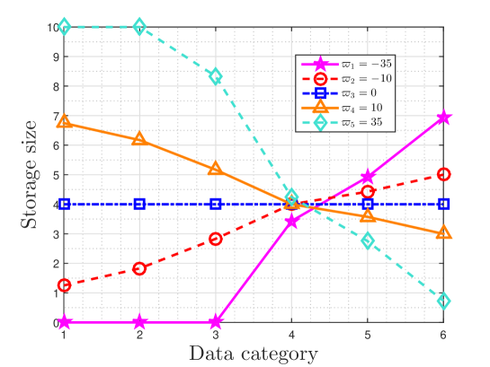
Figure 3: Broken line graph of optimal storage size with the probability distribution $(0.03,0.07,0.1395,0.2205,0.25,0.29)$, for giving maximum available storage size $T=4$ and original storage size $L=10$.

VI-B The Property of the RWRE Based on MIM in Ideal Storage System

Then we focus on the properties of the RWRE. The available storage size $T$ is varying from $0$ to $8$ bits, and the original storage size of each data is $16$ bits. Figure 4 and Figure 5 both present the relationship between the RWRE and the available storage size $\Delta$ with the probability distribution $(0.031,0.052,0.127,0.208,0.582)$.

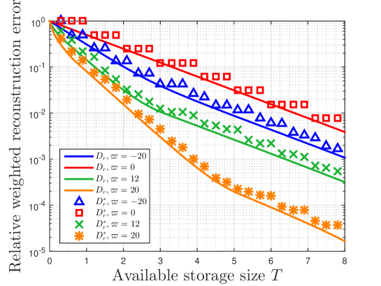
Figure 4: RWRE versus available storage size $T$ with the probability distribution $(0.031,0.052,0.127,0.208,0.582)$ in the case of the value of importance coefficient $\varpi=-20,0,-12,20$. $D_{r}$ is acquired by substituting Equation (18) in Equation (37), while $D_{r}^{*}$ is obtained by substituting Equation (21) in Equation (37).

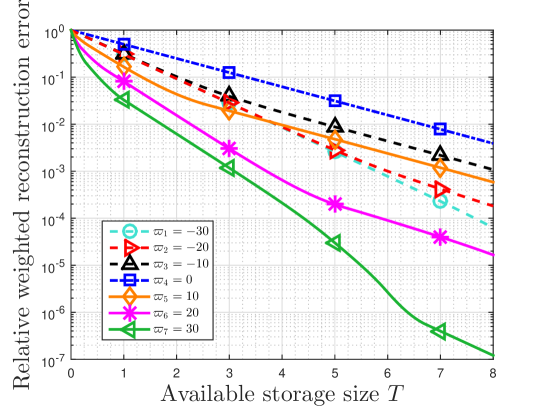
Figure 5: RWRE $D_{r}({\emph{{x}}},\varpi)$ versus available storage size $T$ with the probability distribution $(0.031,0.052,0.127,0.208,0.582)$ in the case of the value of importance coefficient $\varpi=-30,-20,-10,0,10,20,30$.

Figure 4 focuses on the error of RWRE by rounding number with different importance coefficient $\varpi$ ($\varpi=-20,0,-12,20$). In Figure 4, the RWRE $D_{r}$ is acquired by substituting Equation (18) in Equation (37), while the RWRE $D_{r}^{*}$ is obtained by substituting Equation (21) in Equation (37). In this figure, $D_{r}^{*}$ has tierd descent as the available storage size increases, while $D_{r}$ monotonically decreases with increasing of the available storage size. Figure 4 shows that $D_{r}$ is always less than or equal to $D_{r}^{*}$ and they are very close to each other for the same importance coefficient, which means that $D_{r}$ can be used as the lower bound of $D_{r}^{*}$ to reflect the characteristics of $D_{r}^{*}$.

Furthermore, some other observations can be obtained in Figure 5. For the same $T$, the RWRE increases as $\varpi$ increases when $\varpi<0$, while the RWRE decreases with increasing of $\varpi$ when $\varpi>0$. Besides, the RWRE is the largest when $\varpi=0$. It is also observed that the RWRE always decreases with increasing of $T$ for giving $\varpi$. Besides, for any importance coefficient, the RWRE will be $1$ if available storage size is zero. Generally, there is a trade-off between the RWRE and the available storage size, and the results in this paper propose an alternative lossy compression strategy based on message importance.

Then let the importance coefficient $\varpi$ be $5$ and the available storage size $T$ be varying from $2$ to $8$ bits. In addition, the original storage size is still $16$ bits. Besides, the compressed storage size is given by $\Delta=L-T$. In this case, Figure 6 shows that the RWRE versus compressed storage size $\Delta$ for different probability distributions. The probability distributions and some auxiliary variables are listed in Table II. Obviously, all probability distributions satisfy $0\leq T+{\varpi(\gamma_{p}-p_{i})}/{\ln r}\leq L$. It is observed that the RWRE always increases with increasing of $\Delta$ for a giving probability distribution. Some other observations are also obtained. For the same $\Delta$, the RWRE of uniform distribution is the largest all the time. Furthermore, if the RWRE is required to be less than a specified value, which is exceedingly common in actual system in order to make the difference between the raw data and the stored data accepted, the maximum available compressed storage space increases with increasing of $L(\varpi,\emph{{P}})+\varpi e^{-H_{2}(\emph{{P}})}$. Besides, the maximum available compressed storage space is the smallest in uniform distribution. As an example, when the RWRE is required to be smaller than $0.01$, the maximum available compressed storage space of $P_{1}$, $P_{2}$, $P_{3}$, $P_{4}$, $P_{5}$ is $11.85$, $10.97$, $9.99$, $9.73$, $9.36$ respectively. In particular, the maximum available compressed storage size in uniform distribution is the smallest, which suggests the data with uniform distribution is incompressible.

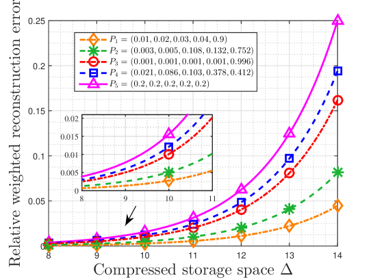
Figure 6: RWRE $D_{r}({\emph{{x}}},\varpi)$ vs. compressed storage size $\Delta$ with importance coefficient $\varpi=5$.

TABLE II: The auxiliary variables in ideal storage system.

Variable	Probability distribution	${\varpi(\gamma_{p}-p_{\alpha_{1}})}/{\ln r}$	${\varpi(\gamma_{p}-p_{\alpha_{2}})}/{\ln r}$	$L(\varpi,\emph{{P}})+\varpi e^{-H_{2}(\emph{{P}})}$
$P_{1}$	$(0.01,0.02,0.03,0.04,0.9)$	5.7924	-0.6276	6.7234
$P_{2}$	$(0.003,0.007,0.108,0.132,0.752)$	4.2679	-1.1350	6.1305
$P_{3}$	$(0.001,0.001,0.001,0.001,0.996)$	7.1487	-0.0287	5.4344
$P_{4}$	$(0.021,0.086,0.103,0.378,0.412)$	2.2367	-0.5838	5.2530
$P_{5}$	$(0.2,0.2,0.2,0.2,0.2)$	0	0	5

VI-C The Property of the RWRE Based on NMIM in Quantification Storage System

Afterwards, Figure 7 presents the relationship between the RWRE and available storage size $T$ for different probability distributions in the quantification storage system. The probability distributions and some auxiliary variables are listed in Table III. Some observations can be obtained. First, the RWRE always decreases with increasing of the available storage size for a giving probability distribution, and there is a trade-off between the RWRE and the available storage size. When the available storage size is small ($T<n/\ln r$), the RWRE decreases largely compared to the case where $T$ is large. Besides, when the maximum available storage size is large ($T>n/\ln r$), the difference between these RWRE remains the same at logarithmic Y-axis. In fact, according to Equation (49), this difference between two probabilities in this figure is the difference of NMIM divided by $\log 10$. As an example, the difference between ${\textbf{\emph{P}}}_{1}$ and ${\textbf{\emph{P}}}_{4}$ in this figure is 30, which satisfies this conclusion for the fact that $(\mathcal{L}({\textbf{\emph{P}}}_{1})-\mathcal{L}({\textbf{\emph{P}}}_{4}))/\log 10\approx 30$. Moreover, the RWRE in ${\textbf{\emph{P}}}_{1}$ is very close to that in ${\textbf{\emph{P}}}_{2}$, and the minimum probabilities in these two probability distributions are the same, i.e., $p_{\alpha_{1}}=0.007$. It suggests that the data with the same minimum probability will have the same compression performance no matter how the distribution changes, if the minimum probability is small. In addition, it is also observed that the RWRE decreases as NMIM $\mathcal{L}({\textbf{\emph{P}}})$ increases for the same $T$, which means this compression strategy is effective in the large NMIM cases.

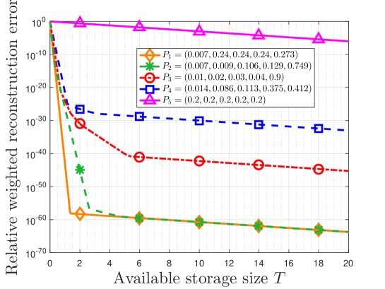
Figure 7: RWRE versus the available storage size $T$.

TABLE III: The auxiliary variables in quantification storage system.

Variable	Probability distribution	$p_{\alpha_{1}}$	$\mathcal{L}({\textbf{\emph{P}}})$
$P_{1}$	$(0.007,0.24,0.24,0.24,0.273)$	0.007	136.8953
$P_{2}$	$(0.007,0.009,0.106,0.129,0.749)$	0.007	136.8953
$P_{3}$	$(0.01,0.02,0.03,0.04,0.9)$	0.01	94.3948
$P_{4}$	$(0.014,0.086,0.113,0.375,0.412)$	0.014	66.1599
$P_{5}$	$(0.2,0.2,0.2,0.2,0.2)$	0.2	4.0000

VII Conclusion

In this paper, we focused on the problem of lossy compression storage from the perspective of message importance when the reconstructed data pursues the least error with certain restricted storage size. We started with importance-weighted reconstruction error to model the compression storage system, and formulated this problem as an optimization problem for digital data based on it. We gave the solutions by a kind of restrictive water-filling, which presented a alternative way to design an effective storage space adaptive allocation strategy. In fact, this optimal allocation strategy prefers to provide more storage size for crucial event classes in order to make rational use of resources, which agrees with the individuals’ cognitive mechanism.

Then, we presented the properties of this strategy based on MIM detailedly. It is obtained that there is a trade-off between the RWRE and available storage size. Moreover, the compression performance of this storage system improves as the absolute value of importance coefficient increases. This is due to the fact that a fraction of data can contain the overwhelming majority of useful information that exerts a tremendous fascination on users as the importance coefficient approaches negative/positive infinity, which suggests that the users’ interest is highly-concentrated. On the other hand, the probability distribution of event classes also has effect on the compression results. When the useful information is only highly enriched in only a small portion of raw data naturally from the viewpoint of users, such as the small-probability event scenarios, it is obvious that we can compress the data greatly with the aid of this characteristics of distribution. Besides, the properties of storage size and RWRE based on non-parametric MIM were also discussed. In fact, the RWRE in the data with uniform information distribution was invariably the largest in any case. Therefore, this paper harbors the idea that the data with uniform information distribution is incompressible, which satisfies the results in information theory.

Proposing more general distortion measure between the raw data and the compressed data, which is no longer only apply to digital data, and using it to acquire the high-efficiency lossy data compression systems from the perspective of message importance are of our future interests.

Appendix A

A-A Proof of Theorem 2

In fact, Equation (24) can be rewritten as

$$l_{i}= \left\{\begin{aligned} &\quad\quad 0\quad\quad\quad\quad\quad\quad\quad\,\,\,\,\,\,\textrm{if}\,\,W_{i}<e^{-\beta\ln r}.\\ &\beta-\frac{-\ln W_{i}}{\ln r}\quad\quad\quad\,\,\quad\quad\textrm{if}\,\,e^{-\beta\ln r}\leq W_{i}\leq e^{(L-\beta)\ln r}.\\ &\quad\quad L\quad\quad\quad\quad\quad\quad\quad\,\,\,\,\,\,\textrm{if}\,\,W_{i}>e^{(L-\beta)\ln r}.\end{aligned}\right.$$ (52)

When $W_{i}>W_{j}$, we have

$$l_{i}-l_{j}= \left\{\begin{aligned} &0\quad\quad\quad\quad\quad\quad\quad\,\,\,\textrm{if}\,\,\,p_{i}>e^{(L-\beta)\ln r},\,\,\,p_{j}>e^{(L-\beta)\ln r}.\\ &L-\beta-\frac{\ln W_{j}}{\ln r}\quad\,\,\,\,\,\textrm{if}\,\,\,p_{i}>e^{(L-\beta)\ln r},\,\,\,e^{-\beta\ln r}\leq p_{j}\leq e^{(L-\beta)\ln r}.\\ &L\quad\quad\quad\quad\quad\quad\,\,\,\,\,\,\,\,\textrm{if}\,\,\,p_{i}>e^{(L-\beta)\ln r},\,\,\,p_{j}<e^{-\beta\ln r}.\\ &\frac{\ln W_{i}-\ln W_{j}}{\ln r}\quad\,\,\,\,\,\,\textrm{if}\,\,\,e^{-\beta\ln r}\leq p_{i}\leq e^{(L-\beta)\ln r},\,\,\,e^{-\beta\ln r}\leq p_{j}\leq e^{(L-\beta)\ln r}.\\ &\beta-\frac{-\ln W_{i}}{\ln r}\quad\quad\,\,\,\,\textrm{if}\,\,\,e^{-\beta\ln r}\leq p_{i}\leq e^{(L-\beta)\ln r},\,\,\,p_{j}<e^{-\beta\ln r}.\\ &0\quad\quad\quad\quad\quad\quad\quad\,\,\,\textrm{if}\,\,\,p_{i}<e^{-\beta\ln r},\,\,\,p_{j}<e^{-\beta\ln r}.\end{aligned}\right.$$ (53)

Due to Equation (8b), we obtain that $0\leq\beta-\frac{-\ln W_{i}}{\ln r}\leq L$, and therefore $L-\beta-\frac{\ln W_{j}}{\ln r}\geq 0$. Besides, it is easy to check that $\frac{\ln W_{i}-\ln W_{j}}{\ln r}$ since that $W_{i}>W_{j}$. Thus, $l_{i}-l_{j}\geq 0$ if $W_{i}>W_{j}$ for $\forall i,j\in\{1,2,...,n\}$. The proof is completed.

A-B Proof of Lemma 1

(1) For $\gamma_{p}$, it is noted that

$$\sum\limits_{i=1}^{n}{p_{i}^{2}}=\frac{1}{n}\left({\sum\limits_{i=1}^{n}{p_{i}^{2}}\sum\limits_{i=1}^{n}{1^{2}}}\right)\geq\frac{1}{n}{{\left(\sum\limits_{i=1}^{n}{p_{i}}\right)}^{2}}=\frac{1}{n},$$ (54)

where the equality holds only if $(p_{1},p_{2},...,p_{n})$ is uniform distribution. Moreover,

$$\sum\nolimits_{i=1}^{n}{p_{i}^{2}}\leq\sum\nolimits_{i=1}^{n}{p_{i}}=1,$$ (55)

where the equality holds only if there is only $p_{t}=1$ ($t\in\{1,2,...,n\}$) and $p_{k}=0$ for $k\neq t$.

(2) For $\gamma_{p}-p_{i}$, we have $\sum\nolimits_{i=1}^{n}p_{i}^{2}-p_{i}\leq\sum\nolimits_{i=1}^{n}p_{i}^{2}\leq 1$. We have equality if and only if $p_{t}=1$ and $p_{i}=0$ for $i\neq t$. Therefore, we only need to check $\sum\nolimits_{i=1}^{n}p_{i}^{2}-p_{i}\geq-1/4$.

First, if $n=1$, we obtain $\sum\nolimits_{i=1}^{n}p_{i}^{2}-p_{i}=0$.

Second, if $n=2$, we obtain $\sum\nolimits_{i=1}^{n}p_{i}^{2}-p_{i}=2(p_{1}-3/4)^{2}-1/8$. It is easy to check that $\sum\nolimits_{i=1}^{n}p_{i}^{2}-p_{i}\geq-1/8$.

Third, if $n>3$, we use the method of Lagrange multipliers. Let

$$J(p)=\sum\limits_{j=1}^{n}p_{j}^{2}-p_{i}-\lambda(\sum\limits_{j=1}^{n}p_{j}-1).$$ (56)

Setting the derivative to $0$, we obtain

$$2p^{*}_{j}-\lambda =0\,\,\,\textrm{for}\,j\neq i$$ (57)

$$2p^{*}_{j}-1-\lambda =0\,\,\,\textrm{for}\,j=i.$$ (57a)

Substituting $p^{*}_{j}$ in the constraint $\sum\nolimits_{j=1}^{n}p^{*}_{j}=1$, we have

$$\frac{\lambda(n-1)}{2}+\frac{\lambda+1}{2}=1.$$ (58)

Hence, we find $\lambda=1/n$ and

$$p^{*}_{j}= \left\{\begin{aligned} &\frac{n+1}{2n}\quad\quad\textrm{if}\,\,j=i,\\ &\frac{1}{2n}\quad\quad\,\quad\textrm{if}\,\,j\neq i.\end{aligned}\right.$$ (59)

In this case, we get

$$\sum\limits_{j=1}^{n}p_{j}^{2}-p_{i}={\frac{n-1}{4n^{2}}}+\frac{{(n+1)}^{2}}{4n^{2}}-\frac{n+1}{2n}=\frac{-n^{2}+n}{4n^{2}}\geq-\frac{1}{4}.$$ (60)

Thus, Lemma 1 is proved.

A-C Proof of Theorem 3

(1) First, let $p_{i}<p_{j}$ when $\varpi>0$. It is noted that

$$W_{i}=\frac{e^{\varpi(1-p_{i})}}{\sum\nolimits_{k=1}^{n}e^{\varpi(1-p_{k})}}>\frac{e^{\varpi(1-p_{j})}}{\sum\nolimits_{k=1}^{n}e^{\varpi(1-p_{k})}}=W_{j}.$$ (61)

Therefore, we find $l_{i}\geq l_{j}$ since that $W_{i}>W_{j}$, due to Theorem 2.

(2) Second, let $p_{i}<p_{j}$ when $\varpi<0$. It is noted that

$$W_{i}=\frac{e^{\varpi(1-p_{i})}}{\sum\nolimits_{k=1}^{n}e^{\varpi(1-p_{k})}}<\frac{e^{\varpi(1-p_{j})}}{\sum\nolimits_{k=1}^{n}e^{\varpi(1-p_{k})}}=W_{j}.$$ (62)

Therefore, we find $l_{i}\leq l_{j}$ since that $W_{i}<W_{j}$, due to Theorem 2. The proof is completed.

A-D Proof of Theorem 4

We define an auxiliary function as

$$f(\varpi)=\frac{\sum\nolimits_{i=1}p_{i}e^{\varpi(1-p_{i})}r^{-l_{i}}}{\sum\nolimits_{j=1}^{n}p_{j}e^{\varpi(1-p_{j})}}.$$ (63)

According to Equation (37), it is noted that the the monotonicity of $D_{r}({\emph{{x}}},\varpi)$ with respect to $\varpi$ is the same with that of $f(\varpi)$.

Without loss of generality, let $l_{i}$ of $p_{i}$ be

$$l_{i}= \left\{\begin{aligned} &\quad\quad\,L\quad\quad\quad\quad\quad\quad\quad\,\,\,\,\,\,\textrm{if}\,\,i=1,2,...,t_{1},\\ &\frac{\ln(\ln r)+\ln W_{i}-\ln\lambda}{\ln r}\quad\textrm{if}\,\,i=t_{1}+1,...,t_{2},\\ &\quad\quad\,0\quad\quad\quad\quad\quad\quad\quad\,\,\,\,\,\,\,\textrm{if}\,\,i=t_{2}+1,t_{2}+2,...,n,\end{aligned}\right.$$ (64)

where $\lambda$ is given by Equation (19) where $\{T_{j},j=1,...,\tilde{N}_{L}\}=\{1,2,...,t_{1}\}$ and $\{I_{j},j=1,...,\tilde{N}\}=\{t_{1}+1,...,t_{2}\}$.

The derivation of $l_{i}$ with respect to $\varpi$ is given by

$$l^{\prime}_{i}= \left\{\begin{aligned} &\frac{\sum\nolimits_{k=t_{1}+1}^{t_{2}}p_{k}(p_{k}-p_{i})}{\ln r(\sum\nolimits_{k=t_{1}+1}^{t_{2}}p_{k})}\quad\,\textrm{if}\,\,\,i=t_{1}+1,...,t_{2}.\\ &\quad\quad 0\quad\quad\quad\quad\quad\quad\,\,\,\quad\textrm{else}.\end{aligned}\right.$$ (65)

Hence,

$$f^{\prime}(\varpi) =\frac{\sum\nolimits_{i}{\sum\nolimits_{j}p_{i}p_{j}{e^{\varpi(2-p_{i}-p_{j})}}r^{-l_{i}}(p_{j}-p_{i}-l^{\prime}_{i}\ln r)}}{{\left(\sum\nolimits_{j}p_{j}e^{\varpi(1-p_{j})}\right)}^{2}}=\frac{F_{1}+F_{2}}{{\left(\sum\nolimits_{j}p_{j}e^{\varpi(1-p_{j})}\right)}^{2}},$$ (66)

where $F_{1}=\sum\nolimits_{j}p_{i}p_{j}{e^{\varpi(2-p_{i}-p_{j})}}r^{-l_{i}}(p_{j}-p_{i})$ and $F_{2}=\sum\nolimits_{j}p_{i}p_{j}{e^{\varpi(2-p_{i}-p_{j})}}r^{-l_{i}}(-l^{\prime}_{i}\ln r)$.

(1) When $\varpi>0$, we have

$$F_{1} =\sum\limits_{p_{j}<p_{i}}p_{i}p_{j}{e^{\varpi(2-p_{i}-p_{j})}}r^{-l_{i}}(p_{j}-p_{i})+\sum\limits_{p_{j}>p_{i}}p_{i}p_{j}{e^{\varpi(2-p_{i}-p_{j})}}r^{-l_{i}}(p_{j}-p_{i})$$ (67)

$$\leq\sum\limits_{p_{j}<p_{i}}p_{i}p_{j}{e^{\varpi(2-p_{i}-p_{j})}}r^{-l_{j}}(p_{j}-p_{i})+\sum\limits_{p_{j}>p_{i}}p_{i}p_{j}{e^{\varpi(2-p_{i}-p_{j})}}r^{-l_{i}}(p_{j}-p_{i})$$ (67a)

$$=\sum\limits_{p_{j}<p_{i}}p_{i}p_{j}{e^{\varpi(2-p_{i}-p_{j})}}r^{-l_{j}}(p_{j}-p_{i})+\sum\limits_{p_{i}>p_{j}}p_{i}p_{j}{e^{\varpi(2-p_{i}-p_{j})}}r^{-l_{j}}(p_{i}-p_{j})$$ (67b)

$$=\sum\limits_{p_{j}<p_{i}}M_{i,j}r^{-l_{j}}(p_{j}-p_{i}+p_{i}-p_{j})$$ (67c)

$$=0.$$ (67d)

In fact, if $p_{i}>p_{j}$, then we will have $l_{i}\leq l_{j}$ due to Theorem 3. Thus, $r^{-l_{i}}(p_{j}-p_{i})\leq r^{-l_{j}}(p_{j}-p_{i})$ in this case. With taking $p_{i}p_{j}{e^{\varpi(2-p_{i}-p_{j})}}\geq 0$ into account, we have Equation (67a). Equation (67b) is obtained by exchanging the notation of subscript in the second item.

For $t_{1}<i\leq t_{2}$ and $1\leq j\leq n$, we have

$$F_{2} =\sum\limits_{i=t_{1}+1}^{t_{2}}\sum\limits_{j=1}^{n}p_{i}p_{j}{e^{\varpi(2-p_{i}-p_{j})}}r^{-l_{i}}(-l^{\prime}_{i}\ln r)$$ (68)

$$=\sum\limits_{i=t_{1}+1}^{t_{2}}\sum\limits_{j=1}^{n}p_{i}p_{j}{e^{\varpi(1-p_{j})-\ln\ln r+\ln\lambda}}(-l^{\prime}_{i}\ln r)$$ (68a)

$$=\sum\limits_{j=1}^{n}\left(p_{j}B_{j}\left(\sum\limits_{i=t_{1}+1}^{t_{2}}p_{i}(-l^{\prime}_{i}\ln r)\right)\right)$$ (68b)

$$=\sum\limits_{j=1}^{n}\left(p_{j}B_{j}\left(\frac{\sum\limits_{i=t_{1}+1}^{t_{2}}p_{i}^{2}\sum\limits_{k=t_{1}+1}^{t_{2}}p_{k}-\sum\limits_{k=t_{1}+1}^{t_{2}}p_{k}^{2}\sum\limits_{i=t_{1}+1}^{t_{2}}p_{i}}{\sum\limits_{k=t_{1}+1}^{t_{2}}p_{k}}\right)\right)$$ (68c)

$$=0,$$ (68d)

where $B_{j}={\textrm{exp}\{{\varpi(1-p_{j})-\ln\ln r+\ln\lambda}}\}$.

Based on the discussions above, we have

$$f^{\prime}(\varpi) =\frac{F_{1}+F_{2}}{{\left(\sum\nolimits_{i=1}^{n}p_{i}e^{\varpi(1-p_{i})}\right)}^{2}}\leq 0.$$ (69)

Since that $f^{\prime}(\varpi)\leq 0$ when $\varpi>0$, $D_{r}({\emph{{x}}},\varpi)$ is monotonically decreasing with $\varpi$ in $(0,+\infty)$.

(2) Similarly, when $\varpi<0$, if $0<p_{j}<p_{i}$, then we will have $l_{i}>l_{j}$ due to Theorem 3. Thus, $r^{-l_{i}}(p_{j}-p_{i})\geq r^{-l_{j}}(p_{j}-p_{i})$ in this case. With taking $p_{i}p_{j}{e^{\varpi(2-p_{i}-p_{j})}}\geq 0$ into account, we have

$$F_{1} \geq\sum\limits_{p_{j}<p_{i}}p_{i}p_{j}{e^{\varpi(2-p_{i}-p_{j})}}r^{-l_{j}}(p_{j}-p_{i})+\sum\limits_{p_{j}>p_{i}}p_{i}p_{j}{e^{\varpi(2-p_{i}-p_{j})}}r^{-l_{i}}(p_{j}-p_{i})$$ (70)

$$=\sum\limits_{p_{j}<p_{i}}p_{i}p_{j}{e^{\varpi(2-p_{i}-p_{j})}}r^{-l_{j}}(p_{j}-p_{i})+\sum\limits_{p_{i}>p_{j}}p_{i}p_{j}{e^{\varpi(2-p_{i}-p_{j})}}r^{-l_{j}}(p_{i}-p_{j})$$ (70a)

$$=\sum\limits_{p_{j}<p_{i}}M_{i,j}r^{-l_{j}}(p_{j}-p_{i}+p_{i}-p_{j})$$ (70b)

$$=0,$$ (70c)

where Equation (70a) is obtained by exchanging the notation of subscript in the second item.

Besides, $F_{2}$ is still given by Equation (68), and $F_{2}=0$. As a result, $f^{\prime}(\varpi)\geq 0$ when $\varpi<0$. Therefore $D_{r}({\emph{{x}}},\varpi)$ is monotonically increasing with $\varpi$ in $(-\infty,0)$.

(3) When $\varpi=0$, the storage size $l_{i}$ for $i=1,2,...,n$ will be all equal to $T$, and therefore $D_{r}({\emph{{x}}},0)=(r^{L-T}-1)/(r^{L}-1)$. Based on the discussion in (1) and (2), we obtain $D_{r}({\emph{{x}}},\varpi)\leq D_{r}({\emph{{x}}},0)$. The proof is completed.

References

• [1] M. Chen, S. Mao, Y. Zhang, and V. C. Leung, Big data: related technologies, challenges and future prospects,   Heidelberg: Springer, 2014.
• [2] H. Cai, B. Xu, L. Jiang, and A. Vasilakos, “IoT-based big data storage systems in cloud computing: perspectives and challenges,” IEEE Internet of Things Journal, vol. 4, no. 1, pp. 75–87, Feb. 2017.
• [3] H. Hu, Y. Wen, T. Chua, and X. Li, “Toward scalable systems for big data analytics: a technology tutorial,” IEEE Access, vol. 2, pp. 652–687, Jun. 2014.
• [4] D. Dong, and J. Herbert, “Content-aware partial compression for textual big data analysis in hadoop,” IEEE Trans. Big Data, vol. 4, no. 4, pp. 459–472, Dec. 2018.
• [5] J. Park, H. Park, and Y. Choi, “Data compression and prediction using machine learning for industrial IoT,” in IEEE ICOIN, Chiang Mai, Thailand, Jan. 2018, pp. 818–820.
• [6] D. Geng, C. Zhang, C. Xia, X. Xia, Q. Liu, and X. Fu, “Big data-based improved data acquisition and storage system for designing industrial data platform,” IEEE Access, vol. 7, pp. 44574 - 44582, Apr. 2019.
• [7] Ö. Nalbantoglu, D. Russell, and K. Sayood, “Data compression concepts and algorithms and their applications to bioinformatics,” Entropy, vol. 12, pp. 34–52, 2010.
• [8] X. Cao, L. Liu, Y. Cheng, and X. Shen, “Towards energy-efficient wireless networking in the big data era: A survey,” IEEE Communications Surveys & Tutorials, vol. 20, no. 1, pp. 303–332, Nov. 2017.
• [9] C.E. Shannon, “A mathematical theory of communication,” Bell Syst. Tech. J., vol. 27, pp. 379–423, 1948.
• [10] Y. Oohama, “Exponential strong converse for source coding with side information at the decoder,” Entropy, vol. 20, doi.org/10.3390/e20050352, 2018.
• [11] F. Pourkamali-Anaraki and S. Becker, “Preconditioned data sparsification for big data with applications to pca and k-means,” IEEE Trans. Inf. Theory, vol. 63, no. 5, pp. 2954–2974, May. 2017.
• [12] I. E. Aguerri and A. Zaidi, “Lossy compression for compute-and-forward in limited backhaul uplink multicell processing,” IEEE Trans. Commun., vol. 64, no. 12, pp. 5227–5238, Dec. 2016.
• [13] T. Cui, L. Chen, and T. Ho, “Distributed distortion optimization for correlated sources with network coding,” IEEE Trans. Commun., vol. 60, no. 5, pp. 1336–1344, May 2012.
• [14] A. Ukil, S. Bandyopadhyay, A. Sinha, and A. Pal, “Adaptive Sensor Data Compression in IoT systems: Sensor data analytics based approach,” in Proc. IEEE ICASSP, Brisbane, Australia, April 2015, pp. 5515–5519.
• [15] J. Zhong, R.D. Yates, and E. Soljanin, “Backlog-adaptive compression: Age of information,” in Proc. IEEE ISIT, Aachen, Germany, June 2017, pp. 566–570.
• [16] C. Elkan, “The foundations of cost-sensitive learning,” in Proc. International Joint Conference on Artificial Intelligence, Seattle, USA, Aug. 2001, pp. 973-978.
• [17] Z. Zhou and X. Liu, “Training cost-sensitive neural networks with methods addressing the class imbalance problem,” IEEE Trans. Knowl. Data Eng., vol. 18, no. 1, pp. 63-77, Jan. 2006.
• [18] S. Lomax and S. Vadera, “A survey of cost-sensitive decision tree induction algorithms,” ACM Computing Surveys (CSUR), vol. 45, no. 2, pp. 16:1-16:35, Feb. 2013.
• [19] B. Masnick and J. Wolf, “On linear unequal error protection codes,” IEEE Trans. Inf. Theory, vol. 3, no. 4, pp. 600–607, Oct. 1967.
• [20] M. Tegmark, and T. Wu, “Pareto-optimal data compression for binary classification tasks,” Entropy, vol. 22, doi.org/10.3390/e22010007, 2020.
• [21] S. Liu, R. She, P. Fan, and K. B. Letaief, “Non-parametric message importance measure: Storage code design and transmission planning for big data,” IEEE Trans. Commun.,, vol. 66, no. 11, pp. 5181 - 5196, Nov. 2018.
• [22] J. Ivanchev, H. Aydt, and A. Knoll, “Information maximizing optimal sensor placement robust against variations of traffic demand based on importance of nodes,” IEEE Trans. Intell. Transp. Syst., vol. 17, no. 3, pp. 714–725, Mar. 2016.
• [23] T. Kawanaka, S. Rokugawa, and H. Yamashita, “Information security in communication network of memory channel considering information importance,” in Proc. IEEE IEEM, Singapore, Singapore, Dec. 2017, pp. 1169–1173.
• [24] K. Sun, and D. Wu, “Unequal error protection for video streaming using delay-aware fountain codes,” in Proc. IEEE ICC, Paris, France, May 2017, pp. 1–6.
• [25] M. Li, W. Zuo, S. GU, D. Zhao, and D. Zhang, “Learning convolutional networks for content-weighted image compression,” in Proc. IEEE CVPR, Salt Lake City, USA, June 2018, pp. 3214–3223.
• [26] X. Zhang and X. Hao, “Research on intrusion detection based on improved combination of K-means and multi-level SVM,” in Proc. IEEE ICCT, Chengdu, China, Oct. 2017, pp. 2042–2045.
• [27] M. Li, “Application of cart decision tree combined with pca algorithm in intrusion detection,” in Proc. IEEE ICSESS, Beijing, China, Nov. 2017, pp. 38-41.
• [28] M.S. Beasley, J.V. Carcello, D.R. Hermanson, and P.D. Lapides, “Fraudulent financial reporting: Consideration of industry traits and corporate governance mechanisms,” Accounting Horizons, vol. 14, no. 234, pp. 441–454, 2000.
• [29] P. Fan, Y. Dong, J. Lu, and S. Liu, “Message importance measure and its application to minority subset detection in big data,” in Proc. IEEE Globecom Workshops, Washington, Dec. 2016, pp. 1–5.
• [30] R. She, S. Liu, S. Wan, K. Xiong, and P. Fan, “Importance of small probability events in big data: information measures, applications, and challenges,” IEEE Access, vol. 7, pp. 100363–100382, Jul. 2019.
• [31] R. She, S. Liu, and P. Fan, “Recognizing Information Feature Variation: Message Importance Transfer Measure and Its Applications in Big Data,” Entropy, vol. 20, no. 6, pp. 1–20, May 2018.
• [32] S. Liu, Y. Dong, P. Fan, R. She, and S. Wan, “Matching users’ preference under target revenue constraints in data recommendation systems,” Entropy, vol. 21, no. 401, doi.org/10.3390/e21020205, 2019.
• [33] T. M. Cover and J. A. Thomas, Elements of information theory, 2nd ed.,   New Jersey, the USA: Wiley, 2006.
• [34] C. C. Aggarwal, Data Classification: Algorithms and Applications,    Boca Raton, FL, USA: CRC Press, 2014.
• [35] J. Salvador–Meneses, Z. Ruiz–Chavez, and J. Garcia–Rodriguez, “Compressed kNN: k-nearest neighbors with data compression,” Entropy, vol. 21, doi:10.3390/e21030234, 2019.
• [36] T. Van Erven and P. Harremoës, “Rényi divergence and kullback-leibler divergence,” IEEE Trans. Inf. Theory, vol. 60, no. 7, pp. 3797–3820, Jul. 2014.