Convexification numerical algorithm for a 2D inverse scattering problem with backscatter data

Abstract

This paper is concerned with the inverse scattering problem which aims to determine the spatially distributed dielectric constant coefficient of the 2D Helmholtz equation from multifrequency backscatter data associated with a single direction of the incident plane wave. We propose a globally convergent convexification numerical algorithm to solve this nonlinear and ill-posed inverse problem. The key advantage of our method over conventional optimization approaches is that it does not require a good first guess about the solution. First, we eliminate the coefficient from the Helmholtz equation using a change of variables. Next, using a truncated expansion with respect to a special Fourier basis, we approximately reformulate the inverse problem as a system of quasilinear elliptic PDEs, which can be numerically solved by a weighted quasi-reversibility approach. The cost functional for the weighted quasi-reversibility method is constructed as a Tikhonov-like functional that involves a Carleman Weight Function. Our numerical study shows that, using a version of the gradient descent method, one can find the minimizer of this Tikhonov-like functional without any advanced a priori knowledge about it.

Keywords. inverse scattering, numerical reconstruction, convexification, backscatter data, Carleman weight function, coefficient identification

AMS subject classification. 35R30, 78A46, 65C20

1 Introduction

Consider the scattering problem for a penetrable inhomogeneous medium in $\mathbb{R}^{2}$. Below ${x}=(x_{1},x_{2})^{T}\in\mathbb{R}^{2}.$ We assume that the scattering object, which occupies a bounded domain in $\mathbb{R}^{2}$, is characterized by the spatially distributed dielectric constant $\varepsilon_{r}(x)=1+a(x)$, where the function $a(x)$ has a compact support. In this paper we are particularly interested in the case of $a(x)\geq 0$ that typically appears in applications of non-destructive testing and explosive detection, see for instance [8, 18, 17] for a similar assumption. Suppose that the object is illuminated by the downward propagating incident plane wave $u_{\mathrm{in}}(x,k)=\exp(ik(d_{1}x_{1}+d_{2}x_{2}))$, where $d_{1}^{2}+d_{2}^{2}=1,d_{2}<0$, the propagation direction $(d_{1},d_{2})^{T}$ is fixed, and $k$ is the wavenumber. Then there arises the scattered wave, and the total wave $u(x,k)$ which is the sum of the incident wave and the scattered wave is governed by the Helmholtz equation as

$$\Delta u+k^{2}(1+a(x))u=0,\quad x\in\mathbb{R}^{2},$$ (1)

$$\lim_{|x|\rightarrow\infty}|x|\left(\frac{\partial(u-u_{\mathrm{in}})}{\partial|x|}-ik(u-u_{\mathrm{in}})\right)=0.$$ (2)

The scattered wave $u-u_{\mathrm{in}}$ satisfies the Sommerfeld radiation condition (2), which guarantees that it behaves like a spherically outgoing wave far away from the scattering object. It is well known that the scattering problem (1)–(2) has a unique solution $u$, see [11]. Now let $R>0$ and consider

$$\Omega=(-R,R)^{2},\quad\Gamma=(-R,R)\times\{R\}.$$

Assume that the scatterer as well as the support of the coefficient $a(x)$ are contained in $\Omega$, and that these objects do not intersect with $\partial\Omega$. Let $\underline{k}$ and $\overline{k}$ be positive constants such that $\underline{k}<\overline{k}$. We consider the following inverse problem.

Inverse Problem. Assume that we are given the multi-frequency backscatter Cauchy data

$$g_{0}(x,k) :=u(x,k),\quad\text{for }{x}\in\Gamma,k\in[\underline{k},\overline{k}],$$ (3)

$$g_{1}(x,k) :=\frac{\partial u}{\partial x_{2}}(x,k),\quad\text{for }{x}\in\Gamma,k\in[\underline{k},\overline{k}],$$ (4)

where the total wave $u(x,k)$ is generated by incident plane waves with a fixed propagation direction. Determine the function $a(x)$ in (1) for $x\in\Omega$, see also Figure 1 for a schematic diagram of the measurement arrangement in the inverse problem.

Uniqueness theorem for this inverse problem can be currently proven only in the case when the right hand side of equation (1) does not equal to zero in $\overline{\Omega}$. This can be done by the so-called Bukhgeim-Klibanov method, which was originated in [8] and is based on applications of Carleman estimates to coefficient inverse problems, see, e.g. [5, 28, 19] for this method. In addition, uniqueness of the approximate problem can be proven when the truncated Fourier series for (1) is used for that approximation, see, e.g. Theorem 3.2 in [15].

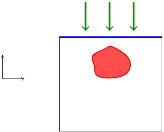
Figure 1: Schematic of the inverse scattering from a penetrable bounded object characterized by the function $a(x)$. The incident plane wave propagates downward toward the scattering object. The backscatter data are measured on the top boundary $\Gamma$ of the computational domain $\Omega$.

This inverse problem belongs to a wider class of coefficient inverse scattering problems which in general aim to recover information about the coefficient $a(x)$ (e.g. its support and/or its values) from the knowledge of the scattered wave generated by a number of incident waves. Inverse scattering problems occur in many applications, including non-destructive testing, explosive detection, medical imaging, radar imaging and geophysical exploration. There is a vast literature about theoretical results and numerical solution to inverse scattering problems, see for instance [11] and references therein. Due to the interest of this paper, we discuss only some numerical methods. The conventional approach is based on the optimization based methods, see, e.g. [2, 10, 13, 14, 12]. However, it is well known that these methods may suffer from multiple local minima and ravines and their convergence analysis is also unknown in many situations. An important attempt in overcoming the drawbacks of the optimization based methods is the qualitative approach which aims to compute the geometry of the scattering object or the support of the coefficient $a(x)$. We refer to [9, 16, 11] and references therein for the development of qualitative methods in solving inverse scattering problems. Although one may be able to avoid local minima or the use of advanced a priori information of the solution, still only geometrical information of the scatterer can be reconstructed with qualitative methods. Furthermore, these methods typically require muti-static data which are sometimes not available in practical applications.

The numerical method proposed in this paper is an extended study from a recent new approach called globally convergent numerical methods (GCNM) for solving coefficient inverse problems. We say that a numerical method for a nonlinear ill-posed problem converges globally if there is a rigorous guarantee that it delivers points in a sufficiently small neighborhood of the exact solution of this problem without any advanced knowledge of this neighborhood. The GCNM typically aims to reconstruct a coefficient in an inverse scattering problem using scattering data either for a single direction of the incident plane wave, or, most recently, for many locations of the point source but at a fixed single frequency [15]. An interesting feature of GCNM is that in all cases the data are non over-determined. The latter means that the number $m$ of free variables in the data equals the number $n$ of free variables in the unknown coefficient, $m=n$. The main advantage of the GCNM is that any version of it avoids the local minimum problem suffered by optimization based methods. Still, any version of GCNM holds the above indicated global convergence property. We refer to [5, 27, 33, 29, 34] and references therein for theoretical results as well as numerical and experimental data study of the first type of GCNM.

The method of this paper is inspired by the second type of the GCNM, which is called convexification. The development of the convexification has started in 1995 and 1997 by Klibanov [18, 17] and continued since then in [6, 28, 22]. However, those were mostly analytical works since some obstacles existed at that time on the path to the numerical implementation, although see some numerical results for the one-dimensional case in [28]. Fortunately, in 2017 the work [1] has eliminated those obstacles. This generated a number of more recent publications on the convexification [25, 24, 21, 26, 23, 15], which contain both a rigorous convergence analysis and numerical results. In particular, publications [25, 24] are about the verification of the convexification on experimental data.

The central idea of the convexification is to construct of a globally convex weighted Tikhonov-like functional with the Carleman Weight Function in it. The idea of the use of the Carleman Weight Function is an unexpected consequence of the original idea of the Bukhgeim-Klibanov method [8], which was originally aimed only for proofs of uniqueness theorems for coefficient inverse problems. The final step of the convergence analysis of the convexification consists in the proof of the global convergence of the gradient projection method to the exact solution, as long as the level of noise in the data tends to zero. We also refer to another version of the convexification, which has started in the work [3] and has been continued in [4, 7, 31]. Carleman Weight Functions are also a crucial element of these works. The main difference between these publications and our method is that it is assumed in [3, 4, 7, 31] that the initial condition in a hyperbolic/parabolic PDE is not vanishing in $\overline{\Omega}$, which unlike our case of the zero right hand side of equation (1).

As to this present paper, our first step is to eliminate the coefficient from the Helmholtz equation using a change of variables. Next, using a truncated Fourier expansion for a function generated by the total wave field, we approximately reformulate the inverse problem as the Cauchy problem for a system of quasilinear elliptic PDEs. The Cauchy boundary data are as follows: on a part of the boundary both Dirichlet and Neumann boundary data are given and no data are given on the rest of the boundary. We then propose a weighted quasi-reversibility method to solve the problem. Inspired by the concept of the convexification, the cost functional in that weighted quasi-reversibility method contains a Carleman Weight Function. This function plays the decisive role in the numerical performance of the method. A method of gradient descent type is explored to find the global minimizer of the cost functional without using any advanced a priori information about it.

Comparing with the above cited recent works on the convexification, the new features of this work are that firstly our algorithm exploits the new Fourier basis in [21] to solve a multi-dimensional inverse problem for the Helmholtz equation with multifrequency data and a single direction of the incident plane wave. The latter is mostly related to [25] in which, however, only the one-dimensional version of the inverse problem has been studied. Using the new Fourier basis from [21], the 3D inverse problem for the Helmholtz equation with data generated by a moving source (at a fixed frequency) has been also studied in [15]. Secondly, a modification during the iteration of the gradient descent method is applied to help the cost functional converge faster. More precisely, we solve the direct problem to update some functions during the iterations of the gradient descent method. Thirdly, unlike the previous works [25, 24, 21, 26, 23, 15], the reconstruction algorithm proposed in this paper works without using any data completion process, and the numerical study covers challenging cases of scattering objects of different shapes which are characterized by different values of the dielectric constant. We also want to mention that the implementation of the method uses a full $H^{2}$ term instead of $L^{2}$ or $H^{1}$ terms as in the previous works cited above and does not need any cut-off and averaging procedures during the iteration in the algorithm.

The convergence analysis of the method of this paper will be addressed in an incoming publication. To be more precise, we now roughly (i.e. without some details) specify what kind of theorems will be proven in that publication. Analogs of these theorems for the one-dimensional case can be found in [25]. Those theorems claim:

1. The strict convexity of the weighted Tikhonov-like functional $\mathcal{J}(W)$ in (19) on the ball $B(M)\subset\mathcal{X}$ of the radius $M$, see (17) and (18). The strict convexity will be proven for sufficiently large values of the parameter $\lambda\geq\lambda(M)\geq 1$ in the Carleman Weight Function (20).

2. Existence and uniqueness of the minimizer of the functional $\mathcal{J}(W)$ on $\overline{B(M)}$ for $\lambda\geq\lambda(M)$.

3. Convergence of the gradient projection method of the minimization of the functional $\mathcal{J}(W)$ on $\overline{B(M)}$ to the exact solution of that approximate coefficient inverse problem if starting from an arbitrary point of $B(M)$. That convergence takes place as long as the level of noise in the data tends to zero.

Since the radius $M>0$ of the ball $B(M)$ is an arbitrary number, then this is the desired global convergence property, as defined above. Note that even though the theory requires the parameter $\lambda$ to be sufficiently large, the numerical experience of this and all previous publications about the convexification [25, 24, 21, 26, 23, 15] shows that actually reasonable values of $\lambda$ provide accurate solutions of considered inverse problems.

The paper is structured as follows. The second section is dedicated to the formulation of the inverse problem as an approximate quasilinear elliptic PDE system. The numerical reconstruction method for solving the inverse problem is proposed in Section 3. The implementation and numerical examples of the reconstruction method are presented in Section 4. Finally, Section 5 contains a summary discussion of this work.

2 An approximate elliptic PDE formulation

In this section we reduce our inverse problem to the Cauchy problem for a system of quasilinear elliptic PDEs that we will be studying using a quasi-reversibility approach in the next section. The main ideas for deriving the formulation are using truncated Fourier expansion in $L^{2}(\underline{k},\overline{k})$ and eliminating the coefficient $a(x)$ from the scattering problem. Setting $k_{0}=(\underline{k}+\overline{k})/2$ we first need the following important Fourier basis of $L^{2}(\underline{k},\overline{k})$ that was introduced in [21]

$$\psi_{n}(k)=(k-k_{0})^{n-1}e^{k-k_{0}},\quad k\in(\underline{k},\overline{k}),\quad n=1,2,\dots$$

Applying the Gram–Schmidt process to $(\psi_{n})$ we obtain an orthonormal basis $\left\{\Phi_{n}\right\}_{n=1}^{\infty},$ which has the following properties, also, see [21]:
i) $\Phi_{n}\in C^{\infty}[\underline{k},\overline{k}]$ for all $n=1,2,...$
ii) The matrix $D=[d_{mn}]$, where $m,n=1,\dots,N$ and

$$d_{mn}=\int_{\underline{k}}^{\overline{k}}\Phi_{n}^{\prime}(k)\Phi_{n}(k)dk,$$

is invertible with $d_{mn}=1$ for $m=n$ and $d_{mn}=0$ for $m>n$.

Now setting

$$p(x,k)=\frac{u(x,k)}{u_{\mathrm{in}}(x,k)},$$ (5)

and substituting in (1) we obtain

$$\Delta p(x,k)+k^{2}a(x)p(x,k)-2ik\partial_{x_{2}}p(x,k)=0.$$ (6)

Now suppose that $p(x,k)$ is nonzero for all $x\in\Omega,k\in[\underline{k},\overline{k}]$. We define $v(x,k)$ as

$$v(x,k)=\frac{\log(p(x,k))}{k^{2}},$$ (7)

where $\log$ is the principal logarithm. We also assume that $v(x,k)$ is continuous and differentiable for all $x\in\Omega,k\in[\underline{k},\overline{k}]$. We refer to [15, 24, 23] for the definition of the complex logarithm for a similar change of variables using a high frequency asymptotic behavior for the total field in $\mathbb{R}^{3}$. Next, this definition was extended in [15] to non high values of $k$ as long as $v(x,k)\neq 0$ for those values. To what we know, that asymptotic behavior is not established yet for the two-dimensional case. At the same time, in our numerical studies, we do not see any discontinuity problem with the principal $\log$.

Using (7) we substitute $p=\exp(k^{2}v)$ in (6) and rewrite (6) in terms of $v(x,k)$ as follows

$$\Delta v(x,k)+k^{2}\nabla v(x,k)\cdot\nabla v(x,k)-2ik\partial_{x_{2}}v(x,k)+a(x)=0.$$ (8)

We now eliminate $a(x)$ by differentiating (8) with respect to $k$

$$\Delta(\partial_{k}v)+2k\nabla v\cdot\nabla(v+k\partial_{k}v)-2i\left(\partial_{x_{2}}v+k\partial_{x_{2}}\partial_{k}v\right)=0.$$ (9)

Let $N\in\mathbb{N}$ be sufficiently large. We approximate the function $v(x,k)$ in (7) and its partial derivative $\partial_{k}v(x,k)$ using the truncated Fourier series as

$$v(x,k)=\sum_{n=1}^{N}v_{n}(x)\Phi_{n}(k),\quad\partial_{k}v(x,k)=\sum_{n=1}^{N}v_{n}(x)\Phi_{n}^{\prime}(k),$$ (10)

where the coefficients $v_{n}(x)$ are given by

$$v_{n}(x)=\int_{\underline{k}}^{\overline{k}}v(x,k)\Phi_{n}(k)dk.$$ (11)

Using two truncated series (10), we approximate (9) by

$$\sum_{n=1}^{N}\Phi_{n}^{\prime}(k)\Delta v_{n}(x)+2k\sum_{n=1}^{N}\sum_{l=1}^{N}\Phi_{n}(k)(\Phi_{l}(k)+k\Phi_{l}^{\prime}(k))\nabla v_{n}(x)\cdot\nabla v_{l}(x)$$

$$-2i\sum_{n=1}^{N}(\Phi_{n}(k)+k\Phi_{n}^{\prime}(k))\partial_{x_{2}}v_{n}(x) =0.$$

For each $m=1,\dots,N$, multiplying both sides of the above equation by $\Phi_{m}(k)$ and integrating with respect to $k$ over $[\underline{k},\overline{k}]$, we obtain

$$\sum_{n=1}^{N}\left(\int_{\underline{k}}^{\overline{k}}\Phi_{m}(k)\Phi_{n}^{\prime}(k)dk\right)\Delta v_{n}(x)\\ +\sum_{n=1}^{N}\sum_{l=1}^{N}\left(2k\int_{\underline{k}}^{\overline{k}}\Phi_{m}(k)\Phi_{n}(k)\left[\Phi_{l}(k)+k\Phi_{l}^{\prime}(k)\right]dk\right)\nabla v_{n}(x)\cdot\nabla v_{l}(x)\\ -\sum_{n=1}^{N}\left(2i\int_{\underline{k}}^{\overline{k}}\Phi_{m}(k)\left[\Phi_{n}(k)+k\Phi_{n}^{\prime}(k)\right]dk\right)\partial_{x_{2}}v_{n}(x)=0.$$ (12)

Considering two $N\times N$ matrices defined as

$$D =(d_{mn}),\quad d_{mn}=\int_{\underline{k}}^{\overline{k}}\Phi_{m}(k)\Phi_{n}^{\prime}(k)dk,$$

$$S =(s_{mn}),\quad s_{mn}=-2i\int_{\underline{k}}^{\overline{k}}\Phi_{m}(k)\left[\Phi_{n}(k)+k\Phi_{n}^{\prime}(k)\right]dk,$$

and an $N\times N$ block matrix $B=(B_{mn})$, each block $B_{mn}=(b_{mn}^{(l)})_{l}$ is an $N\times 1$ matrix defined as

$$b_{mn}^{(l)}=2k\int_{\underline{k}}^{\overline{k}}\Phi_{m}(k)\Phi_{n}(k)\left[\Phi_{l}(k)+k\Phi_{l}^{\prime}(k)\right]dk,$$

we can rewrite (12) as a system of PDEs for the vector valued function $V(x)=[v_{1}(x)\ v_{2}(x)\ \dots\ v_{N}(x)]^{T}$

$$D\Delta V(x)+B\partial_{x_{1}}V(x)\bullet\partial_{x_{1}}V(x)+B\partial_{x_{2}}V(x)\bullet\partial_{x_{2}}V(x)+S\partial_{x_{2}}V(x)=0.$$ (13)

Here the operator $\bullet$ is defined as follows: If $P=(P_{m})$ is an $N\times 1$ block matrix, each block $P_{m}$ is an $N$-dimensional column vector and $V$ is an $N$-dimensional column vector then $P\bullet V$ is an $N$-dimensional column vector given by

$$P\bullet V=\begin{bmatrix}P_{1}\cdot V\\ P_{2}\cdot V\\ \vdots\\ P_{N}\cdot V\end{bmatrix}.$$

Defining

$$\mathcal{Q}(V)=D\Delta V+B\partial_{x_{1}}V\bullet\partial_{x_{1}}V+B\partial_{x_{2}}V\bullet\partial_{x_{2}}V+S\partial_{x_{2}}V,$$

we are able to approximately reformulate the inverse problem as the Cauchy problem for the following system of quasilinear elliptic PDEs:

$$\mathcal{Q}(V) =0\quad\text{in}\ \Omega,$$ (14)

$$V =G_{0}\quad\text{on}\ \Gamma,$$ (15)

$$\partial_{x_{2}}V =G_{1}\quad\text{on}\ \Gamma,$$ (16)

where $G_{0}$ and $G_{1}$ can be computed from the given boundary data $g_{0}$ and $g_{1}$ in (3)–(4) using (5), (7) and (11). If we can find $V$ by solving problem (14)–(16), the coefficient of interest $a(x)$ can be approximately recovered from (8).

Remark 1

We emphasize that the reconstruction algorithm we study in the next section for solving problem (14)–(16) only needs the backscatter data on $\Gamma$. In contrast, the convexification method of above cited papers [25, 24, 21, 26, 23, 15], one has to artificially complete the backscatter data on the other boundaries of $\Omega$ for a better stability of computations. On the other hand, the forthcoming analytical results that are mentioned in Introduction for this paper are valid with the Carleman Weight Function (20) only if the Dirichlet data for the system (14) are known on the entire boundary $\partial\Omega$ rather than just on its part $\Gamma$, i.e. they are valid for those completed data. Thus, our claim in the first sentence of this Remark is based only on our numerical observation and is not supported by the theory. Nevertheless, this numerical observation emphasizes the stability property of our method.

Remark 2

It is well known that the Cauchy problem for an elliptic equation is unstable. Thus, we actually construct a regularization method of solving this problem for our case. A similar numerical method was constructed in [20] for ill-posed Cauchy problems for a wide class of single quasilinear PDEs, including the elliptic one. However, the Carleman Weight Function used in [20] for the elliptic case is inconvenient for the numerical implementation since it depends on two large parameters, instead of just one in our case of (20).

3 A numerical reconstruction algorithm

We solve problem (14)–(16) using the weighted quasi-reversibility method. We first make a change of variables to have homogeneous boundary conditions on $\Gamma$. Let $F$ be a vector valued function which satisfies the boundary conditions (15)–(16). We call $F$ the data carrier and its construction is detailed in the numerical study section. Assuming $V$ is the solution of problem (14)–(16), we define

$$W=V-F.$$

Then $W$ satisfies the homogeneous boundary conditions on $\Gamma$, that is,

$$W=\partial_{x_{2}}W=0\quad\text{on}\ \Gamma.$$

Define the function space $\mathcal{X}$ as

$$\mathcal{X}=\left\{W\in[H^{2}(\Omega)]^{N},\ W=\partial_{x_{2}}W=0\ \text{on}\ \Gamma\right\}$$ (17)

with its associated norm

$$\lVert W\rVert_{\mathcal{X}}=\left(\sum_{n=1}^{N}\lVert w_{n}\rVert_{H^{2}(\Omega)}^{2}\right)^{\frac{1}{2}},\quad\text{where }W(x)=[w_{1}(x)\ w_{2}(x)\ \dots\ w_{N}(x)]^{T}.$$

Let $M>0$ be an arbitrary number. Define the ball $B(M)\subset\mathcal{X}$ as

$$B(M)=\left\{W\in\mathcal{X}:\left\|W\right\|_{\mathcal{X}}<M\right\}\subset\mathcal{X}.$$ (18)

Next, we define the weighted Tikhonov-like functional $\mathcal{J}:B(M)\rightarrow\mathbb{R}$ as

$$\mathcal{J}(W)=\int_{\Omega}\lvert\mathcal{Q}(W+F)\rvert^{2}\varphi^{2}dx+\rho\lVert W\rVert_{\mathcal{X}}^{2}+\alpha_{1}\int_{\Gamma}\lvert W\rvert^{2}dx+\alpha_{2}\int_{\Gamma}\left|\partial_{x_{2}}{W}\right|^{2}dx,$$ (19)

where

$$\varphi(x)=e^{-\lambda(x_{2}-s)^{2}}$$ (20)

is a Carleman Weight function and $\lambda\geq 1$ and $s>R$ are constants. From our numerical experience, the regularization terms involving $\alpha_{1}$ and $\alpha_{2}$ help us obtain better stability for the computation although they are not needed in the theory of convexification methods in previous studies [25, 24, 21, 26, 23, 15]. Below we focus on the minimization of the functional $\mathcal{J}(W)$ on the ball $B(M)\subset\mathcal{X}$ defined in (18). As stated in Introduction, the use of the Carleman Weight Function is inspired by convexification methods whose different versions are described in the above cited publications. For the Carleman Weight Function $\varphi$ in (20), a Carleman estimate for the Laplacian has been proved in [26], where the Dirichlet boundary condition is given on the entire boundary of $\Omega$, which requires an artificial complement of the backscatter data given only on the part $\Gamma$ of $\partial\Omega$. Actually, assigning the Dirichlet data on the entire boundary $\partial\Omega$, one provides an additional stability property to the method. Recall that (see Remark 1) it is our numerical observation that our algorithm only requires the backscatter data on the top boundary $\Gamma$ of $\Omega$.

An interesting numerical observation is that our algorithm converges and provides better reconstruction results with the Carleman Weight Function, as compared with the case when this function is absent in (19), i.e. when $\lambda=0$ in (20): compare Figure 2 and Figure 3 for numerical results with and without the Carleman Weight Function. The two parameters $\lambda$ and $s$ along with the regularization parameters $\rho$, $\alpha_{1}$, $\alpha_{2}$ will be chosen numerically in the implementation of the algorithm. We find the solution $W$ as the global minimizer of $\mathcal{J}(W)$ using a method of gradient descent type. We point out that even though we can prove the global convergence on $B(M)$ of the gradient projection method rather than of the gradient descent method, still our numerical observation is that the latter method has good convergence properties. The same observation took place in all previous publications about the convexification where numerical results were presented [25, 24, 21, 26, 23, 15]. This is a quite useful observation since the numerical implementation of the gradient descent method is much simpler than the one of the gradient projection method.

In the following we describe our numerical algorithm for finding the coefficient $a(x)$ for the inverse problem in (3)–(4), in which finding the minimizer $W$ of $\mathcal{J}(W)$ is one of the main components of the algorithm.

Remark 3

In this algorithm, we recall that the capital letter notations, for example $W(x)=[w_{1}(x)\ w_{2}(x)\ \dots\ w_{N}(x)]^{T}$, are vector valued functions whose components are Fourier coefficients of the corresponding scalar function

$$w(x,k)=\sum_{n=1}^{N}w_{n}(x)\Phi_{n}(k)$$

with the normal letter notations. We also prescribe a tolerance which forces our iteration to stop after the cost functional no longer decreases much. The tolerance will be chosen numerically in the implementation of the algorithm.

The numerical reconstruction algorithm

Step 1.

Construct the data carrier $F$. Set the initial guess $V_{0}:=F$ then proceed into the main iteration (Step 2).

Step 2a.

Set $W_{n}:=V_{n}-F$, compute the cost functional $\mathcal{J}(W_{n})$ and its gradient $\nabla\mathcal{J}(W_{n})$.

• If $n\geq 1$ and $|\mathcal{J}(W_{n})-\mathcal{J}(W_{n-1})|<tolerance$, stop the iteration and move to Step 3.

• Otherwise proceed to Step 2b.

Step 2b.

• Set $\tilde{W}_{n}:=W_{n}-\varepsilon\nabla\mathcal{J}(W_{n})$, where the gradient descent step size $\varepsilon$ is chosen numerically.

• Set $\tilde{V}_{n}:=\tilde{W}_{n}+F$ and compute the corresponding scalar function $\tilde{v}_{n}$.

• Compute $a_{n}(x)$ from $\tilde{v}_{n}$ using the real part of (8) with $k=\underline{k}$.

• Compute $u(x,k)$ by solving the direct problem (1)–(2) with $a(x):=a_{n}(x)$, and set $u_{n+1}(x,k):=u(x,k)$.

• Compute $v_{n+1}(x,k)$ from $u_{n+1}(x,k)$ using (5) and (7), and then compute $V_{n+1}$.

• Set $n:=n+1$ and return to Step 2a.

Step 3.

Set $V:=V_{n}$, compute $v(x,k)$ from $V$ and compute $a(x)$ using the real part of (8) with $k=\underline{k}$.

Remark 4

We observe from the numerical performance of the algorithm that solving the direct problem to update $V_{n}$ helps the cost functional decrease faster with respect to iterations. This is important to the algorithm since the cost functional decreases very slowly after the first iteration without this update.

4 Numerical study

In this section, we describe some important details of the numerical implementation of the above algorithm and present some numerical reconstruction results. The first step of the algorithm is to construct the data carrier $F$. Recall that our computational domain $\Omega=(-R,R)^{2}$. For $0<\xi<R$, define the $\chi_{0}(t),$

$$\chi_{0}(t)=\left\{\begin{array}[]{ll}\text{exp}\left(-\frac{R}{t+\xi}\right),&t>-\xi\\ 0,&t\leq-\xi\end{array}\right.$$

and then set

$$\chi(t)=\frac{\chi_{0}(t)}{\chi_{0}(t)+\chi_{0}(R-t-2\xi)}.$$

Then $\chi(t)=0$ for $-R<t\leq-\xi$, $\chi(t)=1$ for $R-\xi\leq t<R$, and $\chi$ is a smooth transition from $0$ to $1$ on $[-\xi,R-\xi]$. Set

$$f(x,k)=\left[\tilde{g}_{0}(x,k)+(x_{2}-R)\tilde{g}_{1}(x,k)\right]\chi(x_{2}),$$

where $\tilde{g}_{0}$ and $\tilde{g}_{1}$ are the Cauchy data for $v(x,k)$, which means $v=\tilde{g}_{0}$ on $\Gamma$ and $\partial_{x_{2}}v=\tilde{g}_{1}$ on $\Gamma$. Obviously, these data can be computed from the data $g_{0}$ and $g_{1}$ in (3)–(4) using the relation between $u$ and $v$ in (5) and (7). Then the function $f$ satisfies the boundary conditions $f=\tilde{g}_{0}$ on $\Gamma$ and $\partial_{x_{2}}f=\tilde{g}_{1}$ on $\Gamma$. Thus, the corresponding vector valued function $F(x)=[f_{1}(x)\ f_{2}(x)\ \dots\ f_{N}(x)]^{T}$ containing the Fourier coefficients of $f$ with respect to that truncated Fourier basis satisfies the boundary conditions (15)–(16). Actually by the definition of $\chi$ the function $f(x,k)$ is zero in $(-R,-\xi]$, which means that we mainly seek for the scattering object in the upper part $(-R,R)\times[-\xi,R)$ of the square $\Omega$ since the Cauchy data are given on the top boundary $\Gamma$. Indeed, since the Cauchy problem (14)–(16) is unstable, then it is unlikely that even after the regularization, which we do here, one could image scattering objects well, if they are located far from the measurement side $\Gamma$. For the parameter $\xi$ we choose $\xi=R/10$ in the numerical implementation.

For the implementation of the algorithm, we first discretize the computational domain $\Omega$ into $(N_{x}+1)\times(N_{x}+1)$ uniform grid points $x_{ij}=(x_{j},y_{i}),1\leq i,j\leq N_{x}+1$, where the mesh size is $h_{x}$. The wave number interval $[\underline{k},\overline{k}]$ is divided into $N_{k}$ uniform subintervals, where $k_{1},k_{2},\dots,k_{N_{k}}$ are the midpoints and $h_{k}$ is the length of each subinterval. Define the lined up index as follows

$$\mathfrak{m}=\mathfrak{m}(i,j,r)=i+(j-1)(N_{x}+1)+(r-1)(N_{x}+1)^{2},\quad 1\leq i,j\leq N_{x}+1,\ 1\leq r\leq N.$$

In this section, using the lined up index $\mathfrak{m,}$ we write vector valued functions at grid points $x_{ij}$ as a column vector without changing notations. For instance, for $U(x)=[u_{1}(x)\ u_{2}(x)\ \dots\ u_{N}(x)]^{T}$, we have

$$U=[u_{\mathfrak{m}}],\quad 1\leq\mathfrak{m}\leq(N_{x}+1)^{2}N,$$

where

$$u_{\mathfrak{m}}=u_{\mathfrak{m}(i,j,r)}=u_{r}(x_{ij}).$$

Let $\hat{W}=W+F$ and set $W=[w_{\mathfrak{m}}]$ and $\hat{W}=[\hat{w}_{\mathfrak{m}}]$. The weighted Tikhonov-like functional $\mathcal{J}$ in (19) is discretized using finite differences as

$$\mathcal{J}(W) =h_{x}^{2}\sum_{m=1}^{N}\sum_{j=2}^{N_{x}}\sum_{i=2}^{N_{x}}\left|\sum_{r=1}^{N}\left[\frac{d_{mr}}{h_{x}^{2}}\left(\hat{w}_{\mathfrak{m}(i+1,j,r)}+\hat{w}_{\mathfrak{m}(i-1,j,r)}+\hat{w}_{\mathfrak{m}(i,j+1,r)}+\hat{w}_{\mathfrak{m}(i,j-1,r)}-4\hat{w}_{\mathfrak{m}(i,j,r)}\right)\right.\right.$$

$$\quad+\sum_{s=1}^{N}\frac{b_{mr}^{s}}{h_{x}^{2}}\left(\hat{w}_{\mathfrak{m}(i,j+1,r)}-\hat{w}_{\mathfrak{m}(i,j,r)}\right)\left(\hat{w}_{\mathfrak{m}(i,j+1,s)}-\hat{w}_{\mathfrak{m}(i,j,s)}\right)$$

$$\quad+\sum_{s=1}^{N}\frac{b_{mr}^{s}}{h_{x}^{2}}\left(\hat{w}_{\mathfrak{m}(i+1,j,r)}-\hat{w}_{\mathfrak{m}(i,j,r)}\right)\left(\hat{w}_{\mathfrak{m}(i+1,j,s)}-\hat{w}_{\mathfrak{m}(i,j,s)}\right)$$

$$\quad+\left.\left.\frac{s_{mr}}{h_{x}}\left(\hat{w}_{\mathfrak{m}(i+1,j,r)}-\hat{w}_{\mathfrak{m}(i,j,r)}\right)\right]\varphi(x_{ij})\right|^{2}$$

$$+\rho h_{x}^{2}\sum_{m=1}^{N}\sum_{j=1}^{N_{x}+1}\sum_{i=1}^{N_{x}+1}\left|w_{\mathfrak{m}(i,j,m)}\right|^{2}$$

$$+\rho h_{x}^{2}\sum_{m=1}^{N}\sum_{j=2}^{N_{x}}\sum_{i=2}^{N_{x}}\left[\left|\frac{w_{\mathfrak{m}(i,j+1,m)}-w_{\mathfrak{m}(i,j,m)}}{h_{x}}\right|^{2}+\left|\frac{w_{\mathfrak{m}(i+1,j,m)}-w_{\mathfrak{m}(i,j,m)}}{h_{x}}\right|^{2}\right.$$

$$\quad+\left|\frac{w_{\mathfrak{m}(i,j+1,m)}-2w_{\mathfrak{m}(i,j,m)}+w_{\mathfrak{m}(i,j-1,m)}}{h_{x}^{2}}\right|^{2}+\left|\frac{w_{\mathfrak{m}(i+1,j,m)}-2w_{\mathfrak{m}(i,j,m)}+w_{\mathfrak{m}(i-1,j,m)}}{h_{x}^{2}}\right|^{2}$$

$$\quad+\left.2\left|\frac{w_{\mathfrak{m}(i+1,j+1,m)}-w_{\mathfrak{m}(i-1,j+1,m)}-w_{\mathfrak{m}(i+1,j-1,m)}+w_{\mathfrak{m}(i-1,j-1,m)}}{h_{x}^{2}}\right|^{2}\right]$$

$$+\alpha_{1}h_{x}\sum_{m=1}^{N}\sum_{j=1}^{N_{x}+1}\left|w_{\mathfrak{m}(N_{x}+1,j,m)}\right|^{2}+\alpha_{2}h_{x}\sum_{m=1}^{N}\sum_{j=2}^{N_{x}}\left|\frac{w_{\mathfrak{m}(N_{x}+1,j,m)}-w_{\mathfrak{m}(N_{x},j,m)}}{h_{x}}\right|^{2}.$$

We now describe how to compute $\nabla\mathcal{J}(W)$ for complex valued vector function $W$. Recall that if $z$ is a complex variable, $\mathbf{z}=(z_{1},z_{2},\dots,z_{M})$ is a complex vector and $h(\mathbf{z})$ is a complex valued function then we have (see [30])

$$i.\quad\frac{\partial}{\partial z}|z|^{2}=\frac{\partial}{\partial z}(z\bar{z})=\bar{z},$$

$$ii.\quad\frac{\partial h}{\partial\mathbf{z}}(\mathbf{z})=\left[\frac{\partial h}{\partial z_{1}}\ \frac{\partial h}{\partial z_{2}}\ \dots\ \frac{\partial h}{\partial z_{M}}\right],$$

$$iii.\quad\nabla h(\mathbf{z})=\left(\overline{\frac{\partial h}{\partial\mathbf{z}}(\mathbf{z})}\right)^{T}.$$

Thus, by the chain rule we have

$$\frac{\partial}{\partial\mathbf{z}}|h|^{2}(\mathbf{z})=\overline{h(\mathbf{z})}\ \frac{\partial h}{\partial\mathbf{z}}(\mathbf{z}).$$

Treating $\mathcal{J}(W)$ as a function of $(N_{x}+1)^{2}N$ complex variables and applying all of the above to each of its summands, we are able to compute $\frac{\partial\mathcal{J}}{\partial W}(W)$ and thus obtain $\nabla\mathcal{J}(W)$ using ($iii$).

We need a numerical solver for the direct problem (1)–(2) in Step 2b of the reconstruction algorithm and to generate synthetic scattering data for the numerical study. It is well known that the direct problem (1)–(2) is equivalent to the Lippmann-Schwinger integral equation

$$u(x,k)=u_{\mathrm{in}}(x,k)+k^{2}\int_{\Omega}\frac{i}{4}H_{0}^{(1)}(k\lvert x-y\rvert)a(y)u(y,k)dy,$$ (21)

where $H_{0}^{(1)}$ is the Hankel function of the first kind of order 0, see [11]. We exploit the numerical method studied in [35] to solve this integral equation to generate the Cauchy data $g_{0}(x,k)$ and $g_{1}(x,k)$ for the inverse problem. Note that the numerical method studied in [35] assumes smooth coefficients. Its extension to the case of discontinuous coefficients is studied in [32] which can be adapted to our discontinuous coefficient examples in this section. We also add an artificial random noise to the data

$$g_{j}(x,k)=g_{j}(x,k)+\delta\lVert g_{j}\rVert_{L^{2}}\mathcal{N}_{j}(x,k),\quad j=0,1,$$

where $\delta$ is the noise level and $\mathcal{N}_{j}$ are functions taking random complex values and satisfy $\lVert\mathcal{N}_{j}\rVert_{L^{2}}=1$. We consider $5\%$ noise in the Cauchy backscatter data which means $\delta=0.05$ in our numerical examples.

In all numerical examples presented in this section the computational domain is chosen as $\Omega=(-0.8,0.8)^{2}$, where $N_{x}=28$. This means $\Omega$ is uniformly discretized into $29^{2}$ points. The interval of wave numbers is $k\in[\underline{k},\overline{k}]=[0.5,2]$, where $N_{k}=50$. We have found that $N=4$ in (10) is sufficient for the Fourier series truncation, also, see [15] for a similar choice. We generate the multifrequency data for the incident plane wave

$$u_{\mathrm{in}}(x)=e^{-ikx_{2}},\quad k\in[0.5,2].$$

In the Carleman Weight Function $\varphi(x)$ (20), we choose $\lambda=5,s=1.$ This means that

$$\varphi(x)=e^{-5(x_{2}-1)^{2}}.$$

This choice was made by trial and error, so as choices of all other parameters used in this section. We refer to works on the convexification [25, 24, 21, 26, 23, 15] for choices of smaller $\lambda\in\left[1,3\right]$. As to our choice of $\lambda,$ it seems to give us the optimal results for our numerical examples of this section. The step size $\varepsilon$ of the gradient descent method and the regularization parameters $\rho,\alpha_{1},\alpha_{2}$ were chosen as:

$$\varepsilon=\alpha_{1}=10^{-3},\quad\rho=\alpha_{2}=10^{-5}.$$

The tolerance number of the iterations is set up to be $10^{-3}$. It happens in all our numerical examples that the algorithm stops within 10 iterations. One can observe in the numerical examples that the value of the minimized functional $\mathcal{J}(W)$ does not change much after 8 or 9 iterations. Since we are interested in $a(x)\geq 0$, in the final iteration we assign $a(x)$ to be zero in the area in which it takes negative values. By our numerical experience, this area is typically below the reconstructed scatterer.

It is important to mention that the initial guess $W_{0}\equiv 0$ for $W$ in all numerical examples below. This goes along well with our theory (to be published) which guarantees that our algorithm converges to the correct solution starting from any point of the ball $B(M)$ defined in (18), see item 3 in the end of Introduction. This certainly a significant advantage of our method, compared with locally convergent optimization approaches, which typically need a strong a priori knowledge of the scatterer. Such a knowledge, however, is rarely available in applications.

4.1 Numerical example 1

In this example we consider a single scattering disk characterized by the coefficient $a(x)$ which equals 3 inside the disk and zero elsewhere. We can see from the reconstruction result in Figure 2 that the location and and the maximal value of $a(x)$ are well reconstructed. It seems to us that the shape of the scattering object is not well-reconstructed because the backscatter data are generated by incident plane waves with a fixed direction, also, see [33, 34, 24, 23] for similar results. Convergence of the algorithm can be observed from Figure 2(b). From our numerical experience the cost functional $\mathcal{J}$ does not decrease much after 8 or 9 iterations, see also Figure 2(b).

Now with the numerical result in Figure 3 we want to indicate the importance of the Carleman Weight Function for our numerical algorithm. The algorithm does not converge when the cost functional $\mathcal{J}$ does not involve the Carleman weight function. Firstly, the error between the cost functionals at two consecutive iterations is never smaller than the tolerance number $10^{-3}$ like what we have when the Carleman Weight Function is present. Therefore, the iterations do not stop with the chosen tolerance. Secondly, the cost functional $\mathcal{J}$ starts to increase after a certain number of iterations. Figure 3(a) presents the reconstruction result at the sixth iteration where the cost functional obtains its smallest value among 20 iterations. However, this result is not as good as that of Figure 2(c) where the Carleman Weight Function is involved. Indeed, the artifact in Figure 3(a) is slightly stronger and the reconstructed maximal value is 3.2157 while the maximal value of the reconstruction in Figure 2(c) is 3.0014. Also for the next examples, the reconstruction results are always better with the presence of the Carleman Weight Function in the cost functional.

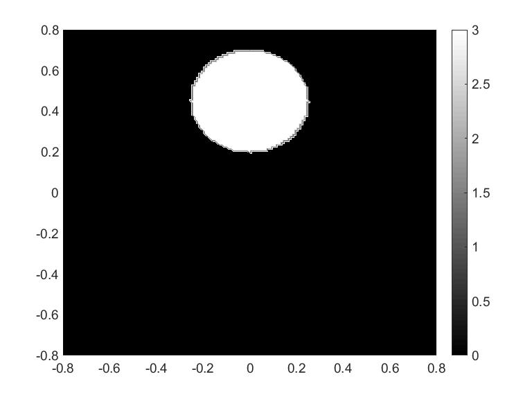
(a) True $a(x)$

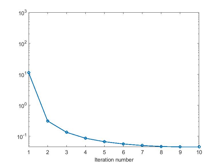
(b) The cost functional

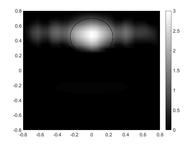
(c) Reconstruction

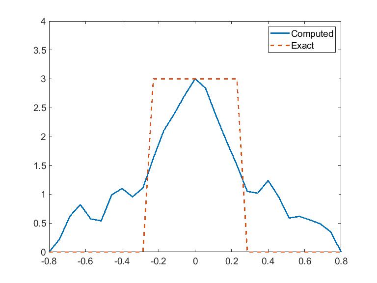
(d) View at $x_{2}=0.45$

Figure 2: Reconstruction of one scattering disk characterized by $a(x)=3$.

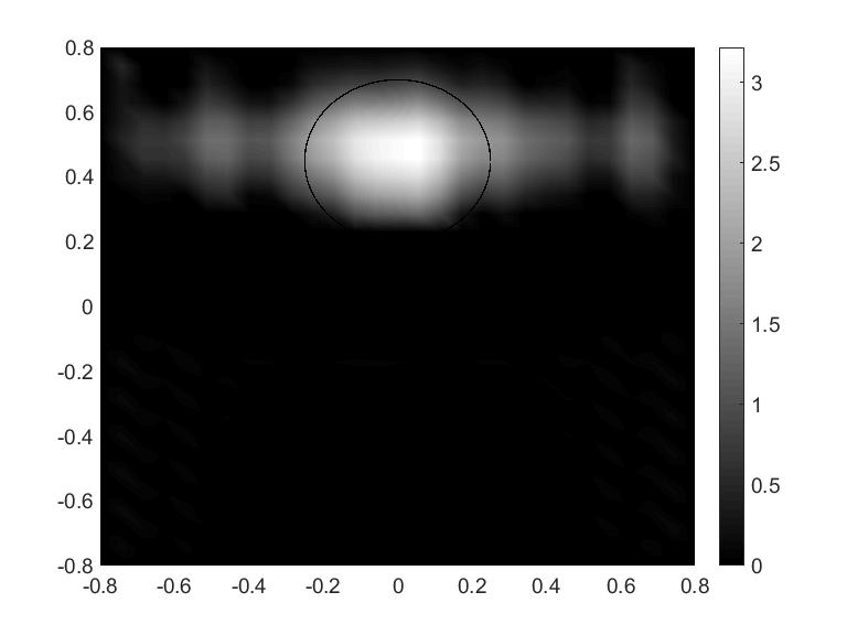
(a) Reconstruction result at the 6th iteration

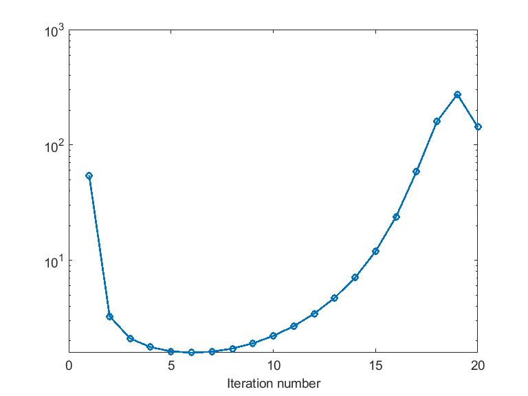
(b) The cost functional

Figure 3: Reconstruction of the scattering disk in Figure 2(a) in which the cost functional does not involve the Carleman Weight Function.

4.2 Numerical example 2

In this example we consider the case of two scattering disks. In the first case in Figure 4(a) two similar scattering disks are considered. The reconstruction result in Figure 4(c) again shows that the algorithm is able to reconstruct very well the location and the maximal values of $a(x)$ in this case. The cost functional decreases well within ten iterations, see Figure 4(b). The case of Figure 5(a) is more challenging since the maximal values of $a(x)$ in each scattering disk are different. However, the algorithm can provide reasonable reconstruction results in Figures 5(c). One can clearly see the locations of the scattering disks as well as two different maximal values of $a(x)$ on each disk. We point out the algorithm in this case can reconstruct the scatterer consisting of two components without using any a priori knowledge about the number of components of the scatterer.

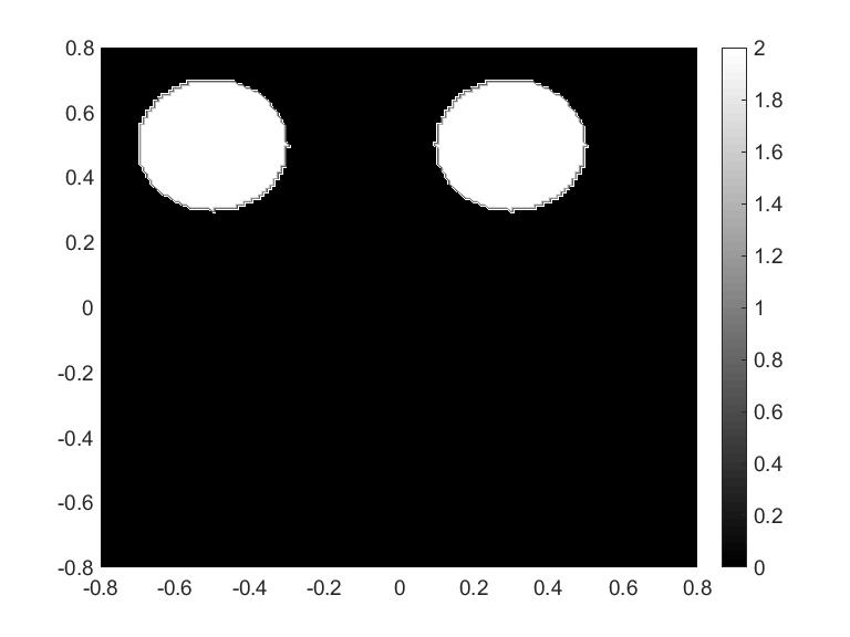
(a) True $a(x)$

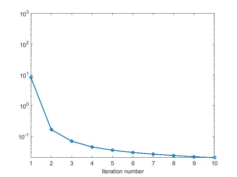
(b) The cost functional

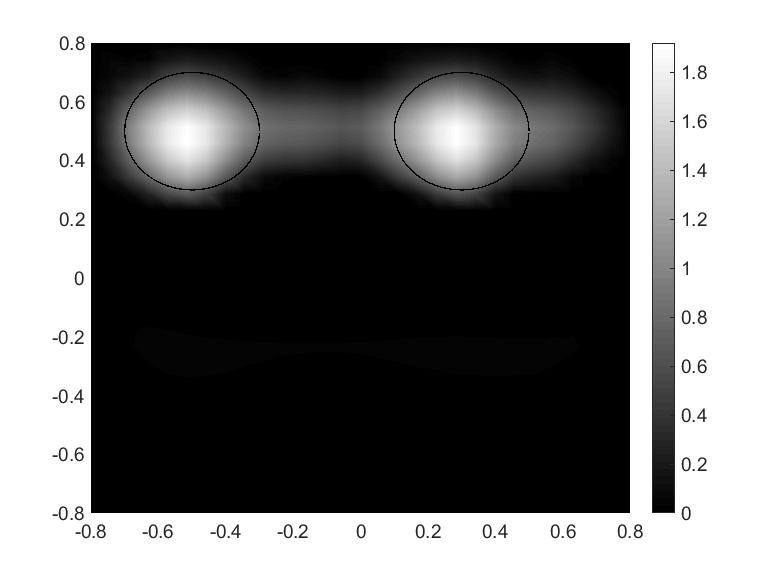
(c) Reconstruction

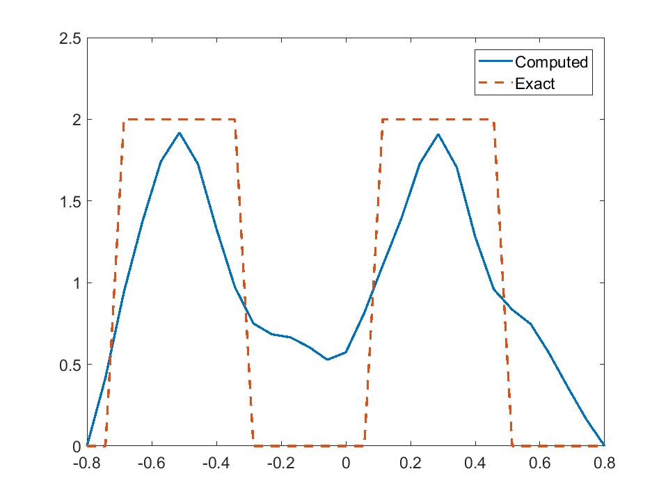
(d) View at $x_{2}=0.45$.

Figure 4: Reconstruction of two similar scattering disks characterized by the coefficient $a(x)=2$.

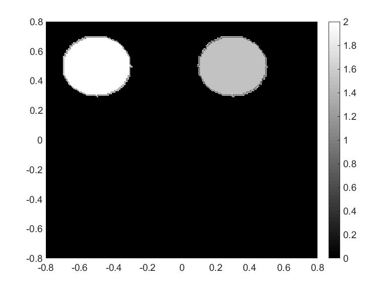
(a) True $a(x)$

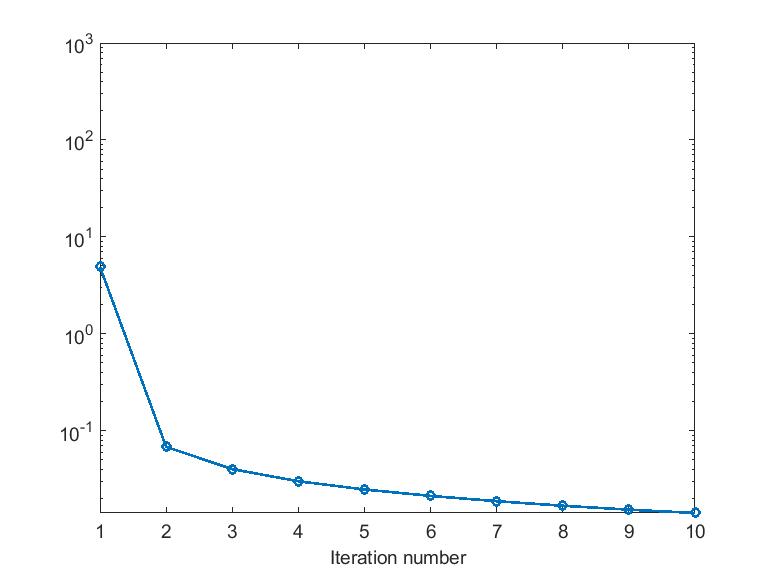
(b) The cost functional

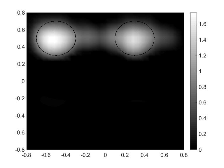
(c) Reconstruction

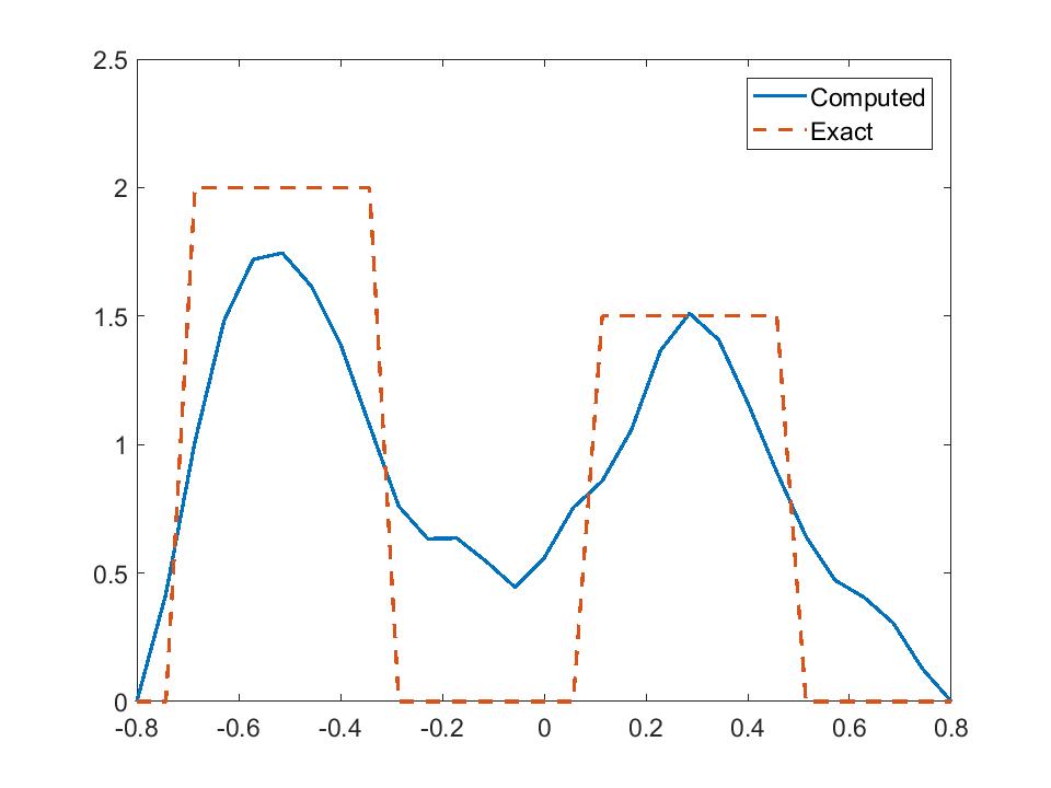
(d) View at $x_{2}=0.45$

Figure 5: Reconstruction of two scattering disks with different values. The coefficient $a(x)=2$ in the left scattering disk and $a(x)=1.5$ in the right scattering disk.

4.3 Numerical example 3

In this example we consider the case of the coefficient $a(x)$ which has different values in scattering objects of different shapes. This case is thus more challenging than those of the first two examples. The scatterer in Figure 6(a) consists of a scattering disk in which $a(x)=2$ and a scattering rectangle in which $a(x)=1.5$. The reconstruction result in Figure 6(c) shows that the algorithm again can compute the location of the scatterer and the maximal values of $a(x)$ in each scattering object. Particularly, we can also see pretty well a difference between the shape of the disk and the rectangle in the reconstruction. The scatterer in Figure 7(a) consists of two scattering disks in which $a(x)=2$ and a scattering rectangle in which $a(x)=1.5$. The reconstruction result in Figure 7(c) provides the location and maximal values of the scattering objects. However, the resolution of the reconstruction in this case is not as good as that of the case of two objects since three scattering objects are placed quite close to each other.

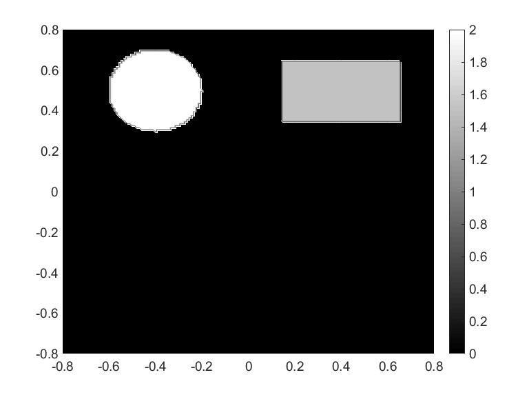
(a) True $a(x)$

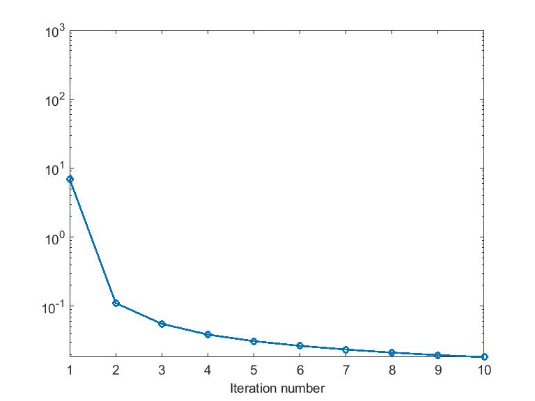
(b) The cost functional

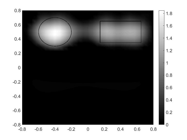
(c) Reconstruction

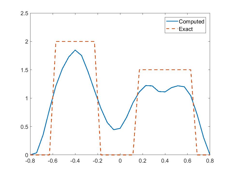
(d) View at $x_{2}=0.45$

Figure 6: Reconstruction of scattering objects with different shapes and values. The coefficient $a(x)=2$ in the left scattering object and $a(x)=1.5$ in the right scattering object.

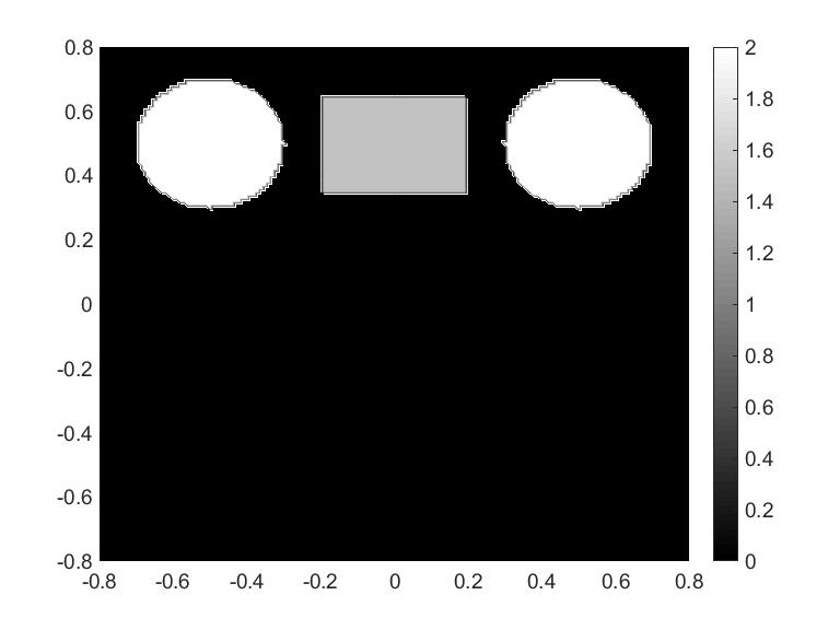
(a) True $a(x)$

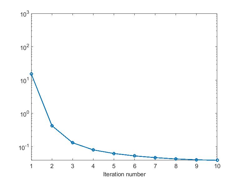
(b) The cost functional

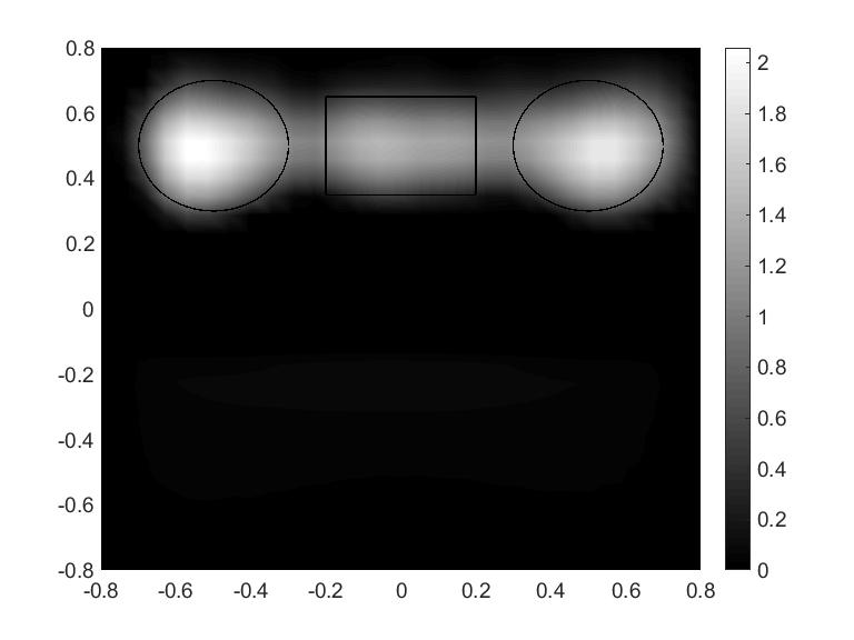
(c) Reconstruction

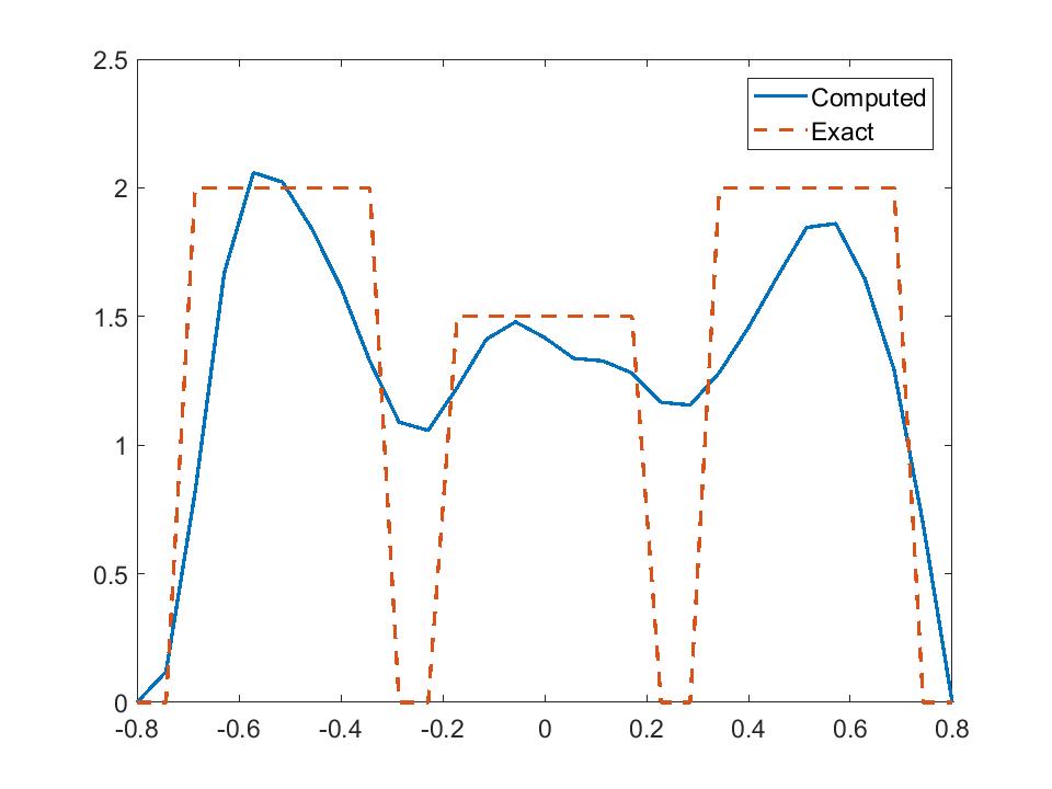
(d) View at $x_{2}=0.45$

Figure 7: Reconstruction of three scattering objects with different shapes and values. The coefficient $a(x)=2$ in the scattering disks and $a(x)=1.5$ in the scattering rectangle.

5 Summary

We have proposed a new version of the convexification numerical reconstruction method for solving the coefficient inverse scattering problem with multifrequency backscatter data associated with a single direction of the incident plane wave. This method relies on an approximate reformulation of the problem as the Cauchy problem for a system of coupled quasilinear elliptic PDEs. The main ingredients for deriving this formulation are the elimination of the coefficient from Helmholtz equation and the use of truncated Fourier expansion for the total field. To solve the quasilinear elliptic PDE system, we use a weighted quasi-reversibility method in which a Carleman Weight Function is included in the weighted Tikhonov-like functional. The numerical results show that our method is able to efficiently compute the solution without using any a priori information about it. We have shown that values of the dielectric constants of scatterers as well as locations of scatterers can be well reconstructed. However, shapes are not reconstructed well. On the other hand, the recent publication [15] shows that all three components of scatterers can be accurately reconstructed in the case when the point source moves along a straight line and frequency is fixed.

Overall, the main advantage of our algorithm, so as other above cited versions of the convexification method, is its rigorously guaranteed global convergence, as opposed to the local convergence of the conventional optimization methods, see Introduction for the definition of the global convergence. Theoretical analysis of the algorithm as well as its three-dimensional extension will be addressed in forthcoming publications. That theoretical analysis will consists in detailed proofs of results announced in items 1-3 of Introduction.

Acknowledgement. The authors are grateful to Loc Nguyen and Khoa Vo from the University of North Carolina at Charlotte for helpful discussions. The first and second authors are partially supported by NSF grant DMS-1812693. The third author is supported by US Army Research Laboratory and US Army Research Office grant W911NF-19-1-0044.

References

- [1] A. B. Bakushinsky, M. V. Klibanov, N. A. Koshev, Carleman weight functions for a globally convergent numerical method for ill-posed Cauchy problems for some quasilinear PDEs, Nonlinear Analysis: Real World Applications 34 (2017) 201–224.
- [2] A. B. Bakushinsky, M. Y. Kokurin, Iterative Methods for Approximate Solutions of Inverse Problems, Springer Verlag, 2004.
- [3] L. Baudouin, M. de Buhan, S. Ervedoza, Convergent algorithm based on carleman estimates for the recovery of a potential in the wave equation, SIAM J. Numer. Anal. 55 (2017) 1578–1613.
- [4] L. Baudouin, M. de Buhan, S. Ervedoza, A. Osses, Carleman-based reconstruction algorithm for the waves, preprint, https://hal.archives-ouvertes.fr/hal-02458787.
- [5] L. Beilina, M. V. Klibanov, Approximate Global Convergence and Adaptivity for Coefficient Inverse Problems, Springer, New York, 2012.
- [6] L. Beilina, M. V. Klibanov, Globally strongly convex cost functional for a coefficient inverse problem, Nonlinear Anal. Real World Appl. 22 (2015) 272–288.
- [7] M. Boulakia, M. de Buhan, E. Schwindt, Numerical reconstruction based on carleman estimates of a source term in a reaction-diffusion equation, preprint, https://hal.archives-ouvertes.fr/hal-02185889.
- [8] A. L. Bukhgeim, M. V. Klibanov, Global uniqueness of a class of multidimensional inverse problems, Soviet Math. Dokl. 24 (1981) 244–247.
- [9] F. Cakoni, D. Colton, Qualitative Methods in Inverse Scattering Theory. An Introduction., Springer, Berlin, 2006.
- [10] G. Chavent, Nonlinear Least Squares for Inverse Problems: Theoretical Foundations and Step-by-Step Guide for Applications, Scientic Computation, Springer, New York, 2009.
- [11] D. L. Colton, R. Kress, Inverse acoustic and electromagnetic scattering theory, 3rd ed., Springer, 2013.
- [12] H. W. Engl, M. Hanke, A. Neubauer, Regularization of inverse problems, Kluwer Acad. Publ., Dordrecht, Netherlands, 1996.
- [13] A. Goncharsky, S. Romanov, A method of solving the coefficient inverse problems of wave tomography, Comput. Math. Appl. 77 (2019) 967–980.
- [14] A. Goncharsky, S. Romanov, S. Seryozhnikov, Low-frequency ultrasonic tomography: mathematical methods and experimental results, Moscow University Physics Bulletin 74 (2019) 43–51.
- [15] V. Khoa, M. V. Klibanov, L. Nguyen, Convexification for a 3D inverse scattering problem with the moving point source, Submitted (arXiv:1911.10289).
- [16] A. Kirsch, N. Grinberg, The Factorization Method for Inverse Problems, Oxford Lecture Series in Mathematics and its Applications 36, Oxford University Press, 2008.
- [17] M. Klibanov, Global convexity in a three-dimensional inverse acoustic problem, SIAM J. Math. Anal. 28 (1997) 1371–1388.
- [18] M. Klibanov, O. Ioussoupova, Uniform strict convexity of a cost functional for three-dimensional inverse scattering problem, SIAM J. Appl. Math. 26 (1995) 147–179.
- [19] M. V. Klibanov, Carleman estimates for global uniqueness, stability and numerical methods for coefficient inverse problems, J. Inverse Ill-Posed Probl. 21 (2013) 477–560.
- [20] M. V. Klibanov, Carleman weight functions for solving ill-posed cauchy problems for quasilinear pdes, Inverse Problems 31 (2015) 125007.
- [21] M. V. Klibanov, Convexification of restricted Dirichlet-to-Neumann map, J. Inverse Ill-Posed Probl. 25 (2017) 669–685.
- [22] M. V. Klibanov, V. G. Kamburg, Globally strictly convex cost functional for an inverse parabolic problem, Math. Meth. Appl. Sci.. 39 (2015) 930–940.
- [23] M. V. Klibanov, A. E. Kolesov, Convexification of a 3-D coefficient inverse scattering problem, Comput. Math. Appl. 77 (2019) 1681–1702.
- [24] M. V. Klibanov, A. E. Kolesov, D.-L. Nguyen, Convexification method for an inverse scattering problem and its performance for experimental backscatter data for buried objects, SIAM J. Imaging Sci. 12 (2019) 576–603.
- [25] M. V. Klibanov, A. E. Kolesov, A. Sullivan, L. Nguyen, A new version of the convexification method for a 1D coefficient inverse problem with experimental data, Inverse Problems 34 (2018) 115014.
- [26] M. V. Klibanov, J. Li, W. Zhang, Convexification for the inversion of a time dependent wave front in a heterogeneous medium, SIAM J. Appl. Math. 79 (2019) 1722–1747.
- [27] M. V. Klibanov, D.-L. Nguyen, L. H. Nguyen, H. Liu, A globally convergent numerical method for a 3D coefficient inverse problem with a single measurement of multi-frequency data, Inverse Probl. Imaging 12 (2018) 493–523.
- [28] M. V. Klibanov, A. Timonov, Carleman Estimates for Coefficient Inverse Problems and Numerical Applications, VSP, Utrecht, 2004.
- [29] A. E. Kolesov, M. V. Klibanov, L. H. Nguyen, D.-L. Nguyen, N. T. Thành, Single measurement experimental data for an inverse medium problem inverted by a multi-frequency globally convergent numerical method, Appl. Numer. Math. 120 (2017) 176–196.
- [30] K. Kreutz-Delgado, The Complex Gradient Operator and the CR Calculus, Tech. rep., ArXiv:0906.4835v1 (2009).
- [31] T. T. Le, L. H. Nguyen, A convergent numerical method to recover the initial condition of nonlinear parabolic equations from lateral cauchy data, preprint, arXiv: 1910.05584.
- [32] A. Lechleiter, D.-L. Nguyen, A trigonometric Galerkin method for volume integral equations arising in TM grating scattering, Adv. Comput. Math. 40 (2014) 1–25.
- [33] D.-L. Nguyen, M. V. Klibanov, L. Nguyen, A. E. Kolesov, M. A. Fiddy, H. Liu, Numerical solution for a coefficient inverse problem with multi-frequency experimental raw data by a globally convergent algorithm, J. Comput. Phys. 345 (2017) 17–32.
- [34] D.-L. Nguyen, M. V. Klibanov, L. H. Nguyen, M. Fiddy, Imaging of buried objects from multi-frequency experimental data using a globally convergent inversion method, J. Inverse Ill-Posed Probl. 26 (2018) 501–522.
- [35] J. Saranen, G. Vainikko, Periodic integral and pseudodifferential equations with numerical approximation, Springer, 2002.