Re-evaluating scaling methods
for distributed parallel systems

Abstract

The paper explains why Amdahl’s Law shall be interpreted specifically for distributed parallel systems and why it generated so many debates, discussions, and abuses. We set up a general model and list many of the terms affecting parallel processing. We scrutinize the validity of neglecting certain terms in different approximations, with special emphasis on the famous scaling laws of parallel processing. We clarify that when using the right interpretation of terms, Amdahl’s Law is the governing law of all kinds of parallel processing. Amdahl’s Law describes among others the history of supercomputing, the inherent performance limitation of the different kinds of parallel processing and it is the basic Law of the ’modern computing’ paradigm, that the computing systems working under extreme computing conditions are desperately needed.

I Introduction

Amdahl in his famous paper [1], even in the title, wanted to draw the attention to that (as he has coined the wording) the Single Processor Approach (SPA) seriously shall limit the achievable computing performance, given that ”the organization of a single computer has reached its limits” and attempted to explain why it was so. Unfortunately, his successors nearly completely misunderstood his intention. Rather than developing ”interconnection of a multiplicity of computers in such a manner as to permit cooperative solution” the followers used his idea only to derive the limitations of computing systems built from components manufactured for the SPA. The successors constructed his famous formula as well, and unfortunately, attributed an inadequate meaning to its terms. The quick technical development suppressed the real intention and meaning of the Law. When the computing needs and possibilities reached the point where the the precise meaning of the Law matters, the incorrect interpretation attributed to its terms did not describe the experiences, giving way to different other ’laws’ and scaling modes. With the proper interpretation, however, we show ”that Amdahl’s Law is one of the few fundamental laws of computing” [2]. Not only of computing, but of all – even computing unrelated – partly parallelized otherwise sequential activities. This paper discusses only the consequences of the idea on scaling of computer systems constructed in SPA; for the idea he was thinking about, see [3, 4, 5].

In section II, the considered scaling methods are shortly reviewed, and some of their consequences discussed. Section II-A, describes Amdahl’s idea shortly: and introduces his famous formula using our notations. In section II-B, we scrutinize the basic idea of the massively parallel processing, Gustafson’s idea. In section II-C we discuss the ”modern scaling law” [6], based on the the recently introduced ”modern computing” [7]; essentially Amdahl’s idea applied to the modern computing systems.

Section III introduces a (by intention strongly simplified and non-technical) model of the parallelized sequential processing. The model visualizes the meaning of the ”parallelizable portion” and enables us to draw the region of validity of the ”strong” and ”weak” scaling methods. As those scaling methods and principles are relevant to all fields of parallel and distributed processing, we demonstrate the application of the presented formalism for different tasks in section IV.

II The scaling methods

The scaling methods used in the field are necessarily approximations to the general model presented in section III. We discuss the nature and validity of those approximations, furthermore introduce the notations and the formalism.

II-A Amdahl’s Law

Amdahl’s Law (called also the ’strong scaling’) is usually formulated with an equation such as

$$S^{-1}=(1-\alpha)+\alpha/N$$ (1)

where $N$ is the number of parallelized code fragments, $\alpha$ is the ratio of the parallelizable fraction to the total (so $(1-\alpha)$ is the ”serial percentage”), $S$ is a measurable speedup. That is, Amdahl’s Law considers a fixed-size problem, and the $\alpha$ portion of the task is distributed to the fellow processors.

When calculating the speedup, one calculates

$$S=\frac{(1-\alpha)+\alpha}{(1-\alpha)+\alpha/N}=\frac{N}{N\cdot(1-\alpha)+\alpha}$$ (2)

However, as expressed in [8]: ”Even though Amdahl’s Law is theoretically correct, the serial percentage is not practically obtainable.” That is, concerning $S$ there is no doubt that it corresponds to the ratio of the measured execution times, for the non-parallelized and the parallelized case, respectively. But, what is the exact interpretation of $\alpha$, and how can it be used?

Unfortunately, Amdahl used $\alpha$ with the meaning ”the fraction of the the number of instructions which permit parallelism” in Fig. 1 he used as an illustration in his paper. The illustration refers to the case when ”around a point corresponding to 25% data management overhead and 10% of the problem operations forced to be sequential”. At that ”point”, there is no place to discuss more subtle details of the performance affecting factors (otherwise mentioned by Amdahl, such as ”boundaries are likely to be irregular; interiors are inhomogenous; computations required may be dependent on the states of the variables at each point; propagation rates of different physical effects may be quite different; the rate of convergence or convergence at all may be strongly dependent on sweeping through the array along different axes on succeeding passes”). It is worth to notice that Amdahl has foreseen issues with ”sparse” calculations (or in general: the role of data transfer); furthermore that the physical size of the computer and the interconnection of the computing units also matters. The latter is crucial in the case of distributed systems.

However, at that time (unlike today [9, 10]) the execution time was strictly determined by the number of the executed instructions. What he wanted to say was ”the fraction of the time spent with executing the instructions which permit parallelism” (at other places the correct expression ”the fraction of the computational load” was used). This (unfortunately formulated) phrase ”has caused nearly three decades of confusion in the parallel processing community. This confusion disappears when we use processing times in the formulations” [8]. On one side, the researchers guessed that Amdahl’s Law was valid only for software (for the executed instructions), and on the other side the other affecting factors, he mentioned but did not discuss in details, were forgotten.

As expressed correctly in [8]: ”For example, if the serial percentage is to be derived from computational experiments, i.e., recording the total parallel elapsed time and the parallel-only elapsed time, then it can contain all overheads, such as communication, synchronization, input/output and memory access. The law offers no help to separate these factors. On the other hand, if we obtain the serial percentage by counting the number of total serial and parallel instructions in a program, then all other overheads are excluded. However, in this case, the predicted speedup may never agree with the experiments.”

Really, one can express $\alpha$ from Eq. (1) in terms measurable experimentally as

$$\alpha=\frac{N}{N-1}\frac{S-1}{S}$$ (3)

That is this $\alpha_{eff}$ value, the effective parallel portion, can be derived from the experimental data for the individual cases. Also, it is useful to express the efficiency with the pseudo-experimentally measurable

$${\color[rgb]{1,.5,0}\leavevmode\hbox to46.65pt{\vbox to19.07pt{\text{[drawing]}}}}=\frac{S}{N}={\color[rgb]{1,.5,0}\leavevmode\hbox to59.67pt{\vbox to25.85pt{\text{[drawing]}}}}=\frac{R_{Max}}{R_{Peak}} E(\large N,\alpha) \frac{1}{{\color[rgb]{1,0,0}\Large N}\cdot(1-\alpha)+\alpha} E(\large N,\alpha) \frac{1}{{\color[rgb]{1,0,0}\Large N}\cdot(1-\alpha)+\alpha}$$ (4)

data, because for many parallelized sequential systems (including the TOP500 supercomputers) the efficiency (as $R_{Max}/R_{Peak}$) and the number of processors $N$ are provided. Reversing the relation, the value of $\alpha_{eff}$ can be calculated as

$${\color[rgb]{1,.5,0}\leavevmode\hbox to42.77pt{\vbox to17.07pt{\text{[drawing]}}}}={\color[rgb]{1,.5,0}\leavevmode\hbox to43.04pt{\vbox to23.9pt{\text{[drawing]}}}} \alpha(E,N) \frac{E\cdot N-1}{E\cdot(N-1)} \alpha(E,N) \frac{E\cdot N-1}{E\cdot(N-1)}$$ (5)

As seen, the efficiency is a two-parameter function (the corresponding surface is shown in Fig. 1), demonstratively underpinning that ”This decay in performance is not a fault of the architecture, but is dictated by the limited parallelism” [11] and that the properly interpreted Amdahl’s Law perfectly describes its dependence on its variables. This proper interpretation also means that Amdahl’s Law (after the pinpointing given in section II-C) shall describe the behavior of systems using a variety of parallelism, see section IV.

II-B Gustafson’s Law

Partly because of the outstanding achievements of the parallelization technology, partly because of the issues around the practical utilization of Amdahl’s Law, the ’weak scaling’ (also called Gustafson’s Law [12]) was also introduced, meaning that the computing resources grow proportionally with the task size. Its formulation was (using our notations)

$$S=(1-\alpha)+\alpha\cdot N$$ (6)

Similarly to the Amdahl’s Law, the efficiency can be derived for the Gustafson’s Law as (compare to Eq. (4))

$${\color[rgb]{1,.5,0}\leavevmode\hbox to42.21pt{\vbox to17.07pt{\text{[drawing]}}}}=\frac{S}{N}={\color[rgb]{1,.5,0}\leavevmode\hbox to45.97pt{\vbox to23.9pt{\text{[drawing]}}}} E(N,\alpha) \alpha+\frac{(1-\alpha)}{N} E(N,\alpha) \alpha+\frac{(1-\alpha)}{N}$$ (7)

From these equations immediately follows that the speedup (the parallelization gain) increases linearly with the number of processors, without limitation. This conclusion was launched amid much fanfare. They imply, however, some more immediate conclusions, such as

• some speedup can be measured even if no processor is present

• the efficiency slightly increases with the number of processors $N$ (the more processors, the better efficacy)

• the non-parallelizable portion of the job either shrinks as the number of processors grows, or despite that, that portion is non-parallelizable, the system distributes it between the $N$ processors

• executing the extra instructions needed by the first processor to organize the joint work needs no time

• all non-payload computing contributions such as communication (including network transfer), synchronization, input/output and memory access take no time

However, an error was made in deriving Eq. (6): the $N-1$ processors are idle waiting while the first one is executing the sequential-only portion. Because of this, the time that serves as the base for calculating the speedup in the case of using $N$ processors

$$T_{N} =(1-\alpha)_{processing}+\alpha\cdot N{\color[rgb]{1,0,0}+(1-\alpha)\cdot(N-1)_{idle}}$$

$$=(1-\alpha)\cdot N+\alpha\cdot N$$

$$=N$$

For the meaning of the terms in [12], the author used the wording ”is the amount of time spent (by a serial processor)”.

That is, before fixing the arithmetic error, impossible conclusions follow, after fixing it, the conceptual error comes to light: the weak scaling assumes that the single-processor efficiency can be transferred to the parallelized sequential subsystems without loss, i.e., that the efficacy of a system comprising $N$ single-thread processors remains the same than that of a single-thread processor. This statement strongly contradicts the experienced ’efficiency’ of the parallelized systems, not speaking about the ’different efficiencies’ [6], see also Fig. 1.

That is, the Gustafson’s Law is simply a misinterpretation of the argument $\alpha$: a simple function form transforms Gustafson’ Law to Amdahl’s Law [8]. After making that transformation, the two (apparently very different) laws become identical. However, as suspected by [8]: ”Gustafson’s formulation gives an illusion that as if N can increase indefinitely”. This illusion led to the moon-shot of targeting to build supercomputers with computing performance well above the feasible (and reasonable) size and may lead to false conclusions in the case of using clouds. The ’real scaling’ also explains why one could not reveal this illusion for decades and why it provoked decades-long debates in the community.

II-C Real scaling

The role of $\alpha$ was theoretically established [13] and the phenomenon itself, that the efficiency (in contrast with Eq. (7)) decreases as the number of the processing units increases, is known since decades [11] (although it was not formulated in the functional form given by Eq. (4)). In the past decades, the theory faded; mainly due to the quick development of the parallelization technology and single-processor performance. The community used the ’weak scaling’ approximation to calculate the expected performance values, in many cases outside its range of validity. The ’gold rush’ for building exascale computers finally made obvious that under the extreme conditions represented by the need of millions of processors the used ’weak scaling’ leads to false conclusions: it ”can be seen in our current situation where the historical ten-year cadence between the attainment of megaflops, teraflops, and petaflops has not been the case for exaflops” [14]. It looks like, however, that in the feasibility studies of supercomputing using parallelized sequential systems an analysis whether building computers of such size is feasible (and reasonable) remained out of sight either in USA [15, 16] or in EU [17] or in Japan [18] or in China [19].

Figure 1 depicts the two-parameter efficiency surface stemming out from Amdahl’s law (see Eq. (4)). On the surface, some measured efficiencies of the present top supercomputers are also depicted, just to illustrate some general rules. To validate the model described in section III the data of the rigorously verified supercomputer database [20] was used, as described in [6]. The High Performance Linpack (HPL) efficiencies are sitting on the surface, while the corresponding High Performance Conjugate Gradients (HPCG) values are much below those values. The conclusion drawn here was that ”the supercomputers have two different efficiencies” [21], because one cannot explain the experience in the frame of the ”classic computing paradigm”.

The $Taihulight$ and $K~{}computer$ stand out from the ”millions core” middle group. Thanks to its 0.3M cores, $K~{}computer$ has the best efficiency for the $HPCG$ benchmark, while $Taihulight$ with its 10M cores the worst one. The middle group follows the rules [6]. For $HPL$ benchmark: the more cores, the lower efficiency. For $HPCG$ benchmark: the ”roofline” [22] of that communication intensity was already reached, all computers have about the same efficiency.

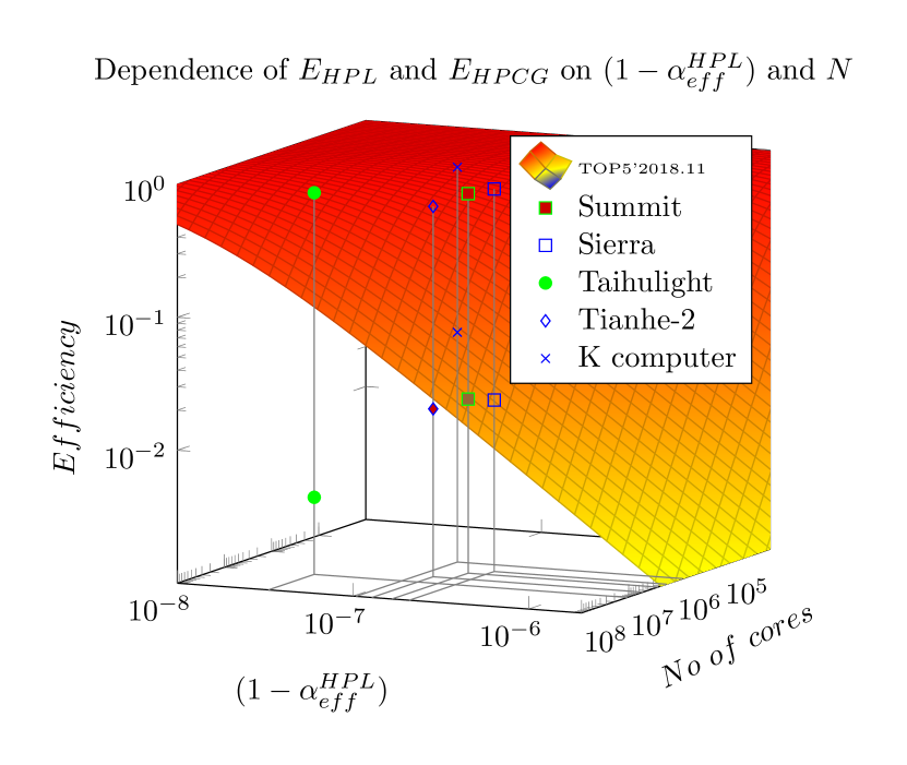
Figure 1: The 2-parameter efficiency surface (in function of the parallelization efficiency measured by benchmark HPL and the number of the processing elements) as concluded from Amdahl’s Law (see Eq. (4)), in the first order approximation. Some sample efficiency values for some selected supercomputers are shown, measured with benchmarks HPL and HPCG, respectively.

According to Eq. (4) the efficiency can be interpreted in terms of $\alpha$ and $N$, and the payload performance of a parallelized sequential computing system can be calculated as

$$P(N,\alpha)=\frac{N\cdot P_{single}}{{N\cdot\left(1-\alpha\right)+\alpha}}$$ (8)

This simple formula explains why the payload performance is not a linear function of the nominal performance and why in the case of very good parallelization ($(1-\alpha)\ll 1$) and low $N$, one cannot notice the nonlinearity. The functional form of the dependence discovers a surprising analogy shown in details in Table I and Fig 2.

TABLE I: The analogy of adding speeds in physics and adding performances in computing, in the classic and modern paradigm, respectively. In both cases a correction term is introduced, that provides noticeable effect only at extremely large values.

Physics Computing Adding of speeds Adding of performance Classic Classic $v(t)={\color[rgb]{0,0,1}t\cdot a}$ $Perf_{total}(N)={\color[rgb]{0,0,1}N\cdot P_{single}}$ t = time N = number of cores a = acceleration $P_{single}=$ Single-performance n = optical density communication c = Light Speed $\alpha$ = parallelism Modern (relativistic) Modern (Amdahl-aware) [7], see Eq. (4) $v(t)=\frac{t\cdot a}{{\color[rgb]{1,.5,0}\leavevmode\hbox to52.83pt{\vbox to23.4pt{\text{[drawing]}}}}}$ $P(N)=\frac{N\cdot P_{single}}{{\color[rgb]{1,.5,0}\leavevmode\hbox to65.05pt{\vbox to17.2pt{\text{[drawing]}}}}}$

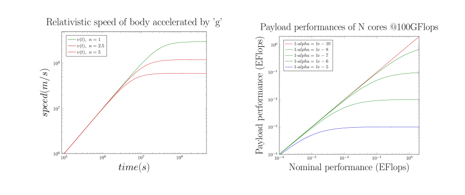
Figure 2: The analogy between how the speed of light changes the linearity of speed dependence at extremely large speed values and that how the value of performance changes the linearity of performance dependence at extremely large performance values.

The right side of Fig. 2 reveals why the nonlinearity of the dependence of the payload performance on the nominal performance was not noticeable earlier: in the age of $1K$ processors, the effect was thousands of times smaller than in the age of $1M$ processors, and the increase seemed to be linear. But anyhow: although one can use the ’weak scaling’ up to around up to a few PFlops (and low communication intensity), it is surely not valid any more. How much the nonlinearity manifests, depends on the type of the workload of the computing system [6]. That is, according Eq. (8) defines the ’real scaling’. The linear approximation (according to the ’weak scaling’) is not valid any more, although it was a good approximation at lower performance values and for shorter extrapolation distances.

Notice that in this section, we assumed that $\alpha$ does not depend on $N$. This assumption is undoubtedly valid for low number of processors, and unquestionably not valid for the cutting-edge supercomputers. That is, as discussed below, the bad news is that the increase of the payload performance is not linear in the function of nominal performance (as would be expected based on ’weak scaling’), but has a performance limit at which it saturates (according to the first-order approximation) or starts to decrease (according to the second-order approximation). The parallelized sequential processing has different rules of game [11], [7]: the performance gain (”the speedup”) has its inherent bounds [6].

III A non-technical model of parallelized sequential operation

To understand why the different ’scaling’ methods are approximations with a limited range of validity; we set up a simple non-technical model.

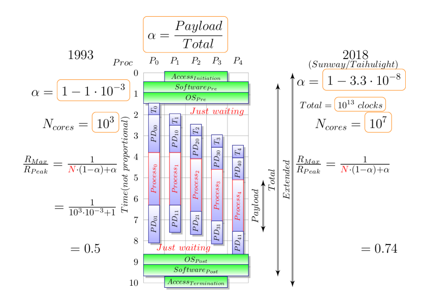
Figure 3: A non-technical, simplified model of parallelized sequential computing operations. The contributions of the model component $XXX$ to $\alpha$ (sometimes used as $\alpha_{eff}$ to emphasize that it is an effective, empirical value) will be denoted by $\alpha_{eff}^{XXX}$ in the text. Notice the different nature of those contributions. They have only one common feature: they all consume time. The vertical scale displays the actual activity for processing units shown on the horizontal scale.

The speedup measurements are simple time measurements (although they need careful handling and proper interpretation, see good textbooks such as [23]): a benchmark executes a standardized set of machine instructions (a large number of times), and divides the known number of operations by the measurement time; for both the single-processor and the distributed parallelized sequential systems. In the latter case, however, the joint work must also be organized, implemented with additional machine instructions and additional execution time, forming an overhead. This additional activity is the origin of the inherent efficiency of the parallelized sequential systems: one of the processors orchestrates the joint operation, the others are idle waiting. At this point, the ”dark performance” appears: the processing units are ready to operate, consume power, but do not make any payload work.

A closer analysis revealed that one of the essential prerequisites to applying Amdahl’s Law is not strictly fulfilled even by the Amdahl’s Law. The reason is that ”It requires the serial algorithm to retain its structure such that the same number of instructions are processed by both the serial and the parallel implementations for the same input” [8]. Because of this, Amdahl’s Law itself is an approximation. In its original form, we can call it the first order approximation to Amdahl’s Law. The approximation takes that compared to the non-parallelizable payload work, organizing the joint work is negligible. The validity of this assumption is limited to a very low number of cores and a relatively high ratio of overhead. Recall that in the age of Amdahl, the non-payload workload ratio was in the range of dozens of percent, so some extra work did not make a considerable difference. Today, as we discuss below, the ratio of the overhead is by orders of magnitude lower, while the number of cores is by orders of magnitude higher (see also the parameters of the different configuration in Fig. 3). This latter aspect we consider as the second order approximation to Amdahl’s Law; for more details see [6].

Amdahl’s idea is to put everything that we cannot parallelize, i.e., distribute between the fellow processing units, into the sequential-only fraction. In the spirit of this idea, for describing the parallel operation of sequentially working units, we prepared the model depicted in Figure 3. The technical implementations of the different parallelization methods show up virtually infinite variety [24], so we present here a (by intention) strongly simplified model. The non-parallelizable contributions are virtually classified (sometimes contracted) and shown as general contribution terms in the figure. In this way, the model is general enough to discuss some case studies of parallelly working systems qualitatively, neglecting different contributions as possible. One can convert the model to a technical (quantitative) one via interpreting the contributions in technical terms, although with some obvious limitations.

As Figure 3 shows, in the parallel operating mode (in addition to the calculation, furthermore the communication of data between the processing units) both the software (in this sense: computation and communication, including data access) and the hardware (interconnection, accelerator latency) contribute to the execution time, i.e., one must consider both of those components in Amdahl’s Law. This statement is not new, again: see [1, 8].

The non-parallelizable (i.e. apparently sequential) part comprises contributions from Hardware (HW), Operating System (OS), Software (SW) and Propagation Delay (PD) (the ”propagation rates of different physical effects”), and also some access time is needed for reaching the parallelized system. This separation is rather conceptual than strict, although dedicated measurements can reveal their role, at least approximately. Some features can be implemented in either SW or HW, or shared between them, and also some sequential activities may happen partly parallel with each other. The relative weights of the contributions are very different for different parallelized systems, and even within those cases depend on many specific factors, so in every single parallelization case, it requires a careful analysis. The SW activity represents what was assumed by Amdahl as the total sequential fraction. What did not yet exist in the age of Amdahl, the non-determinism of the modern HW systems [9] [10] also contributes to the non-parallelizable portion of the task: the slowest unit defines the resulting execution time of the parallelly working processing elements. Also, notice that optimization possibilities are present in the system; for example, see in Fig. 3 how the contribution of classes propagation delay and looping delay can be combined to achieve a better timing.

Our model assumes no interaction between the processes running on the parallelized systems in addition to the necessary minimum: starting and terminating the otherwise independent processes, which take parameters at the beginning and return a result at the end. It can, however, be trivially extended to the more general case when processes must share some resources (like a database, which shall provide different records for the different processes), either implicitly or explicitly. The concurrent objects have their inherent sequentiality [25], and the synchronization and communication between those objects considerably increase [26] the non-parallelizable portion (i.e., contribution to $(1-\alpha_{eff}^{SW})$ or $(1-\alpha_{eff}^{OS})$), so in the case of the massive number of processors, special attention must be devoted to their role on the efficiency of the application on the parallelized system.

In the case of distributed systems, the physical size of the computing system also matters: the processor, connected to the first one with a cable of length of dozens of meters, must spend several hundred clock cycles with waiting, only because of the finite speed of propagation of light, topped by the latency time and hoppings of the interconnection (not mentioning geographically distributed computer systems, such as some clouds, connected through general-purpose networks). This aspect is completely neglected in the ’weak scaling’ approximation. Detailed calculations are given in [27].

After reaching a certain number of processors, there is no more increase in the payload fraction when adding more processors: the first fellow processor already finished the task and is idle waiting, while the last one is still idle waiting for the start command. One can increase this limiting number by organizing the processors into clusters; then, the first computer must speak directly only to the head of the cluster. Another way is to distribute the job near to the processing units, either inside the processor [28] or using processors to let do the job by the processing units of a GPGPU.

This looping contribution is not considerable (and so: not noticeable) at a low number of processing units, but can be a dominating factor at a high number of processing units. This ”high number” was a few dozens at the time of writing the paper [11], today it may be in the order of a few millions. Considering the effect of the looping contribution is the borderline between the first and second-order approximations in modeling the performance: the housekeeping keeps growing with the growing number of processors, while the resulting performance does not increase anymore. Even, the housekeeping gradually becomes the dominating factor of the performance limitation, and leads to a decrease in the payload performance: ”there comes a point when using more processors …increases the execution time rather than reducing it” [11]. That is, the first-order approximation results only in saturated performance; the second-order approximation leads to reaching an inflection point followed by decreasing performance and efficiency.

IV Application fields

According to the model, one expects $(1-\alpha_{eff})$ to describe the fraction of the total (even unintended or only apparently) sequential part in any HW/SW system, and it is a sensitive measure of disturbances and inefficiencies of parallelization [27]. This value can be used as the merit to compare setups, computers manufactured in different ages with different technologies, conditions of network operation, the algorithm for communication within a closed chip, SW load balancing.

In this section (except section IV-E) we assume that the parallelized computing system is accessible in a negligible time, and that the parallelized system under study is properly defined. We do not care whether the one-time contributions (such as initiating the data structures and starting the calculations) are done by the user SW or by the OS; furthermore we assume that we repeat the payload calculation so many times that we can neglect the one-time contributions.

Figure 4: Relative speedup (left side) and ($1-\alpha_{eff}$) (right side) values, measured running the audio and radar processing on different number of cores. [29]

IV-A Load balancing compiler

Today, mainly because of the more and more widespread utilization of multi-core processors, more and more applications are considered to be re-implemented in multi-core aware form. Because it is a serious (and expensive!) effort, before deciding to start such a re-implementation, one needs to guess the speed gain. After finishing the re-implementation, it would be desirable to measure whether we achieved the goal. A method to find out during development, whether we can increase further parallelization using a reasonable amount of development work, would be highly desirable. The achievable speed gain depends on both the structure of the code and the hardware architecture, so one must scrutinize all those aspects.

A compiler making load balancing of an originally sequential code for different number of cores is described and validated in paper [29], by running the executable code on platforms having different numbers of cores. In terms of efficiency, the results they presented have common features and can be discussed together.

The left subfigure of Fig. 4 (Fig 8 in [29]) displays their results in function of the number of cores, using the figure of merit the authors used, the efficiency $E$ (see Equ. (4)). The data displayed in the figures are derived simply through reading back diagram values from the mentioned figures in [29], so they may not be accurate. However, they are accurate enough to support our conclusions.

Their first example shows the results of implementing parallelized processing of an audio stream manually, with an initial (first attempt), and more careful (having already experienced programmers) implementation. For the two different processings of audio streams, using efficiency $E$ as merit enables only to claim a qualitative statement about load balancing, that ”The higher number of parallel processes in Audio-2 gives better results”, because the Audio-2 diagram decreases less steeply than Audio-1. In the first implementation, where the programmer had no previous experience with parallelization, the efficiency quickly drops with the increasing number of cores. In the second round, with experiences from the first implementation, the loss is much less, so $1-E$ rises less speedily.

Their second example is processing radar signals. Without switching in their compiler the load balancing optimization on, the slope of the $1-E$ diagram line is much more significant. It seems to be unavoidable that as the number of cores increases, the efficiency (according to Eq. (4)) decreases, even at such a low number of cores. Both examples leave the questions open whether further improvements are possible or whether the parallelization is uniform in function of the number of cores.

In the right subfigure of Fig. 4 (Fig. 10 in [29]) the diagrams show the $(1-\alpha_{eff})$ values, derived from the same data. In contrast with the left side, these values are nearly constant (at least within the measurement data readback error) which means that the derived merit value is characteristic of the system. By recalling Equ. (1) one can identify this parameter as the resulting non-parallelizable part of the activity, which – even with careful balancing – one cannot distribute between the cores, and cannot be reduced.

In the light of this, one can conclude that both the programmer in the case of audio stream and the compiler in the case of radar signals correctly identified and reduced the amount of non-parallelizable activity. The $\alpha_{eff}$ is practically constant in function of the number of cores, nearly all optimization possibilities found and they hit the wall due to the unavoidable contribution of non-parallelizable software contributions. The better parallelization leads to lower $(1-\alpha_{eff})$ values, and less scatter in the function of the number of cores. The uniformity of the values also make highly probable, that in the case of audio streams further optimization can be done, at least for 6-core and 8-core systems, while the processing of radar signals reached its bounds.

Note that we must not compare the absolute values for analyzing different programs: they represent the sequential-only part of two programs, which may be different. It looks like that the $(1-\alpha_{eff})$ imperfectness can be reduced to about $10^{-1}$ with software methods of parallelization.

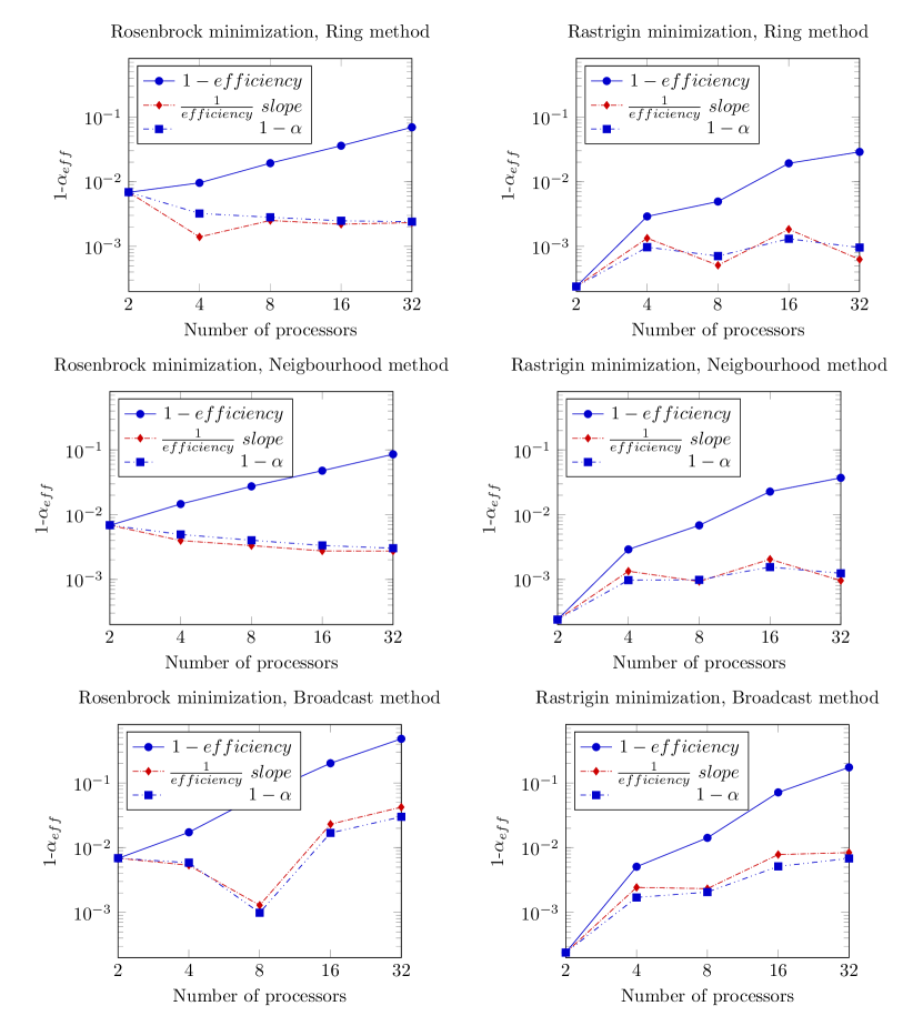
Figure 5: Comparing efficiency, efficiency slope and $\alpha_{eff}$ for different communication strategies when running two minimization task on SoC by [30]

IV-B Measuring the efficiency of the on-chip networking

It is not a trivial task to find out the subtle points of on-chip networking, because of both the limited accessibility and the low number of processing units. The merit developed here, however, can also help in that case; although the available non-dedicated measurements enable us to draw only conclusions of limited accuracy.

In [30] the authors compare different communication strategies their Particle Swarm Optimization (PSO) uses when minimizing Rosenbrock’s function and Rastrigin’s functions, respectively. From their data, we calculated the corresponding $\alpha_{eff}$ values and displayed them in Fig. 5. The fluctuations seen in the figure show the limitations of the (otherwise excellent) measurement precision; for this type of investigation, one would need much longer measurement time.

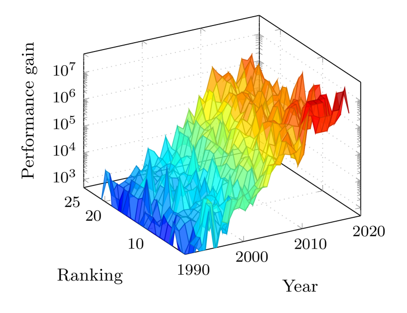
Figure 6: The history of supercomputing in terms of performance gain

The contribution of the OS cannot be separated, again, from SW contribution. Although the precision of the available data does not enable to make a detailed analysis of the behavior of the scaling and to qualify the communication method exhaustively, some observations we can make. When utilizing only two cores, the variety of ways to communicate is minimal. In this case, all communication methods delivered the same $\alpha_{eff}$ value, proving the self-consistency of both the model and the measurement. The values of $\alpha_{eff}$ ($5*10^{-3}$ and $2*10^{-4}$) deviate considerably for the two minimization methods, however. We attribute this deviation to the different structures ($\alpha_{eff}^{SW}$) of the two applications. As the diagrams of the Rastrigin method show, the contribution due to the propagation delay can be in the order of $1*10^{-3}$; which is considerable for the Rastrigin method, but not for the Rosenbrock method. The reason why for higher core numbers is that $\alpha_{eff}$ is nearly constant in the case of the first two communication methods: one of the contributions dominates; although for the Rastrigin method $\alpha_{eff}^{SW}$, while for the Rastrigin method $\alpha_{eff}^{communication}$ is the dominating term.

A bit different is the case for the broadcast-type communication, for both types of minimization methods: the resulting $(1-\alpha_{eff})$ increases with the increasing number of cores. Here the reason is that the number of collisions (and so the time spent with waiting for repeating) increases with the number of cores. This contribution increasingly dominates for the Rastrigin case and increases moderately the already high $(1-\alpha_{eff})$ value at a high number of cores, while at a low number of cores the $(1-\alpha_{eff}^{SW})$ value persists in dominating for the Rosenbrock case.

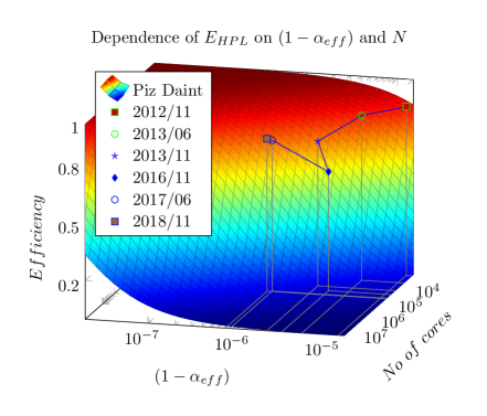
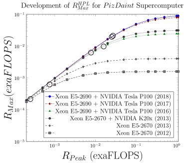
Figure 7: The history of supercomputer Piz Daint in terms of efficiency and payload performance. The left subfigure shows how the efficiency changed as the developers proceeded towards higher performance. The right subfigure shows the reported performance data (the bubbles), together with the diagram line calculated from the value as described above. Compare the value ot the diagram line to the measured performance data in the next reported stage.

IV-C The history of supercomputing

The TOP500 database [20] provides all needed data to calculate $\alpha$, independently from the date of manufacturing, technology, manufacturer, number, and kind of processors. We can use the parallelization efficiency in studying (among others) the history of supercomputing.

During the past quarter of a century, the proportion of the contributions changed considerably: today the number of processors is thousands of times higher than it was a quarter of a century ago. The growing physical size and the higher processing speed increased the role of the propagation overhead, furthermore the large number of processing units strongly amplified the role of the looping overhead. As a result of the technical development, the phenomenon on the performance limitation [11] returned in a technically different form at a much higher number of processors. As discussed, except for an extremely high number of processors, it can be assumed that $\alpha$ is independent from the number of processors. Equ. (5) can be used to derive quickly the value of $\alpha$ from the values of parameters $R_{Max}/R_{Peak}$ and the number of cores $N$.

IV-D The effect technology change in supercomputing

As expressed by Eq. (8), the resulting performance of parallelized computing systems depends on both the single-processor performance and performance gain (mainly the perfectness of the parallelization). To separate these two factors, Fig. 6 displays the performance gain of the supercomputers in the function of their year of construction and the ranking in the given year. The ”hillside” reflects the enormous development of the parallelization technology. Unfortunately, the different individual factors (such as interconnection quality, using accelerators and clustering, or using slightly different computing paradigm) cannot be separated in this way, although even in this figure some limited validity conclusions can be drawn.

One can localize two ’plateaus’ before the year 2000 and after the year 2015, unfortunately, underpinning Amdahl’s Law and refuting Gustafson’s Law. The values between 2000 and 2010 demonstrate the development of the interconnection technology (for a more detailed analysis, see Fig. 6 in [6]). Before 2010 running the benchmark on a top supercomputer was a communication-bound task. Since 2015 it is a computing-bound task. The appearance of accelerators around 2011 caused some ’humps’, and both the excellent clustering and using ’cooperating cores’ [28] increased the achieved performance gain. The wide variety of technical components, manufacturers, interconnections, processors, accelerators, does not enable us to make more detailed connections.

Fortunately, both the validity of the ’real scaling’ and the accuracy of the merit in predicting the future performance values can be demonstrated. The supercomputers usually do not have a long lifespan and several documented stages. One of the rare exceptions is the supercomputer Piz Daint. The documented lifetime spans over 6 years, and during that time, a different number of cores, without and with acceleration, using different accelerators, were used.

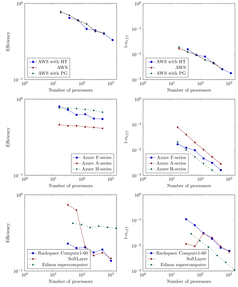
Figure 8: The effect of neglecting the access time when measuring efficiency of some cloud services

Figure 7 depicts the performance and efficiency values published during its lifetime, together with the diagram lines predicting (at the time of making the prediction) the values at the higher nominal performance values. The left subfigure shows how the changes made in the configuration affected the efficiency (the timeline starts in the top right corner, and a line connects the consecutive stages).

In the right subfigure, the bubbles represent data published in the adjacent editions of the TOP500 lists, the diagram lines crossing them are the predictions made from that snapshot. We can compare the predicted values to the value published in the next list. It is especially remarkable that introducing GPGPU acceleration resulted only in a slight increase (in good agreement with [32] and [31]) compared to the value expected based purely on the increase of the number of cores. Between the samplings more than one parameter was changed, that is, we cannot demonstrate the net effect of a change. However, the measured data sufficiently underpin our limited validity conclusions and show that the theory correctly describes the tendency of the development of the performance and the efficiency. The predicted performance values are also reasonably accurate.

Introducing a GPU accelerator is a one-time performance increase step [31], and cannot be taken into account by the theory. Notice that introducing the accelerator increased the payload performance, but decreased the efficiency (copying data from one address space to another increases latency). Changing the accelerator to another type with slightly higher performance (but higher latency due to the larger GPGPU memory) caused a slight decrease in the efficiency.

IV-E The effect of not considering the access time

In [33] the authors benchmarked some commercially available cloud services, fortunately using HPL benchmark. Fig. 8 shows on the left side the efficiency (i.e. $\frac{R_{Max}}{R_{P}eak}$), on the right side, the $(1-\alpha)$ values, in the function of the number of processors in the used configuration. One can immediately notice on one side that the values of $\frac{R_{Max}}{R_{P}eak}$ are considerably lower than unity, even for a very low number of cores. On the other side, the $(1-\alpha)$ values steeply decrease as the number of cores increases, although the model contains only contributions which may only increase as the number of cores increases.

The benchmark HPL characterizes the setup, so the benchmark is chosen correctly. When acquiring measurement data, in the case of clouds, the access time must also be considered, see Fig. 3. If one measures the time on the client’s computer (and this is what is possible using those services), one uses the time Extended in the calculation in place of Total. That is, the ’device under test’ is chosen improperly.

This artifact is responsible for both mentioned differences. The efficiency measured in this way would not achieve 100 % even on a system comprising only one single processor. Since $\alpha$ measures the average utilization of processors, this foreign contribution is divided by the number of processors, so with increasing the number of processors, the relative weight of this foreign contribution decreases, causing to decrease the calculated value of $(1-\alpha)$. Since the access is provided through the Internet where the operation is stochastic, the measurements cannot be as accurate as in purpose-built systems. Some qualitative conclusions of limited validity, however, can be drawn even from those data.

At such a low number of processors neither of the contributions depending on the processor number is considerable, so one can expect that in the case of correct measurement $(1-\alpha)$ would be constant. So, extrapolating the diagram lines of $(1-\alpha)$ to the value corresponding to a one-processor system, one can see that both for Edison supercomputer and Azure A series grid (and maybe also Rackspace) the expected value is approaching unity (but obviously below it). From the slope of the curve (increasing the denominator 1000 times, $(1-\alpha)$ reduces to $10^{-3}$), and one can even find out that $(1-\alpha)$ should be around $10^{-3}$. Based on these data, one can agree with the conclusion that –on a good grid– benchmark HPCG can run as effectively as on the supercomputer they used. One should note, however, that $(1-\alpha)$ is about 3 orders of magnitude better for TOP500 class supercomputers, but this makes a difference only for HPL class benchmarks and only at a large number of processors. This conclusion can be misleading: whether a high-performance cloud can replace a supercomputer in solving a task, strongly depends on the number of cores, because of the different $\alpha$ values.

Note that in the case of AWS grids and Azure F series the $\alpha_{eff}^{OS+SW}$ starts at about $10^{-1}$, and this is reflected by the fact that their efficiency drops quickly as the number of the cores increases. Interesting to note that ranking based on $\alpha$ is just the opposite of the ranking based on efficiency (and strongly correlates with the price of the service).

One can also extrapolate the efficiency values to the point corresponding to one core only. In the case of measurement with no such artifact, the backprojected efficiency value should be around unity. If the measurement artifact is present, it is not the case; the values deviate by a factor up to 2. The back-projected $(1-\alpha)$ values are much more consistent: they tend to hit the value of unity. Sometimes it is lower (meaning some other, foreign, performance loss), but in no case higher than unity.

V Conclusion

The scaling methods, mainly due to their simplicity, can be useful when applied in the range of their validity. Given that they are approximations, we must scrutinize the validity of the omissions periodically. The approximations to the performance of parallelized sequential systems routinely deployed the ’weak scaling’ method to estimate the payload performance of future, ever-larger scale system; without scrutinizing the validity of the method under the current technical situation. However, using this approximation (the incremental development) led to unexpected phenomena, failed supercomputers and unexpectedly low efficiency of the systems. The ’real scaling’ is in complete agreement with the experiences and measured values.

References

- [1] G. M. Amdahl, “Validity of the Single Processor Approach to Achieving Large-Scale Computing Capabilities,” in AFIPS Conference Proceedings, vol. 30, 1967, pp. 483–485.
- [2] J. M. Paul and B. H. Meyer, “Amdahl’s Law Revisited for Single Chip Systems,” International Journal of Parallel Programming, vol. 35, no. 2, pp. 101–123, Apr 2007.
- [3] J. Végh, “Introducing the Explicitly Many-Processor Approach,” Parallel Computing, vol. 75, pp. 28 – 40, 2018.
- [4] J. Végh, “EMPAthY86: A cycle accurate simulator for Explicitly Many-Processor Approach (EMPA) computer.” jul 2016. [Online]. Available: https://github.com/jvegh/EMPAthY86
- [5] ——, “A configurable accelerator for manycores: the Explicitly Many-Processor Approach,” ArXiv e-prints, Jul. 2016. [Online]. Available: http://adsabs.harvard.edu/abs/2016arXiv160701643V
- [6] J. Végh, “Finally, how many efficiencies the supercomputers have?” The Journal of Supercomputing,2020. [Online]. Available: 10.1007/s11227-020-03210-4
- [7] J. Végh and A. Tisan, “The need for modern computing paradigm: Science applied to computing,” in 2019 International Conference on Computational Science and Computational Intelligence (CSCI). IEEE, 2019, p. In print. [Online]. Available: http://arxiv.org/abs/1908.02651
- [8] Y. Shi, “Reevaluating Amdahl’s Law and Gustafson’s Law,” https://www.researchgate.net/publication/ 228367369_Reevaluating_Amdahl’s_law_and_Gustafson’s_law, 1996.
- [9] V. Weaver, D. Terpstra, and S. Moore, “Non-determinism and overcount on modern hardware performance counter implementations,” in Performance Analysis of Systems and Software (ISPASS), 2013 IEEE International Symposium on, April 2013, pp. 215–224.
- [10] P. Molnár and J. Végh, “Measuring Performance of Processor Instructions and Operating System Services in Soft Processor-Based Systems,” in 18th Internat. Carpathian Control Conf. ICCC, 2017, pp. 381–387.
- [11] J. P. Singh, J. L. Hennessy, and A. Gupta, “Scaling parallel programs for multiprocessors: Methodology and examples,” Computer, vol. 26, no. 7, pp. 42–50, Jul. 1993.
- [12] J. L. Gustafson, “Reevaluating Amdahl’s Law,” Commun. ACM, vol. 31, no. 5, pp. 532–533, May 1988.
- [13] A. H. Karp and H. P. Flatt, “Measuring Parallel Processor Performance,” Commun. ACM, vol. 33, no. 5, pp. 539–543, May 1990.
- [14] M. Feldman, “Exascale Is Not Your Grandfather’s HPC,” https://www.nextplatform.com/2019/10/22/exascale-is-not-your-grandfathers-hpc/, 2019.
-
[15]
US Government NSA and DOE, “A Report from the NSA-DOE Technical Meeting on
High Performance Computing,” https://www.nitrd.gov/
nitrdgroups/images/b/b4/NSA_DOE_HPC_TechMeetingReport.pdf, December 2016. - [16] R. F. Service, “Design for U.S. exascale computer takes shape,” Science, vol. 359, pp. 617–618, 2018.
- [17] European Commission, “Implementation of the Action Plan for the European High-Performance Computing strategy,” http://ec.europa.eu/newsroom/dae/document.cfm? doc_id=15269, 2016.
- [18] Extremtech, “ Japan Tests Silicon for Exascale Computing in 2021.” https://www.extremetech.com/computing/ 272558-japan-tests-silicon-for-exascale-computing -in-2021, 2018.
- [19] Liao, Xiang-ke et al, “Moving from exascale to zettascale computing: challenges and techniques,” Frontiers of Information Technology & Electronic Engineering, vol. 19, no. 10, p. 1236–1244, Oct 2018. [Online]. Available: https://doi.org/10.1631/FITEE.1800494
- [20] TOP500, “November 2017 list of supercomputers,” https://www.top500.org/lists/2017/11/, 2017.
- [21] IEEE Spectrum, “Two Different Top500 Supercomputing Benchmarks Show Two Different Top Supercomputers,” https://spectrum.ieee.org/tech-talk/computing/hardware/two-different-top500-supercomputing- benchmarks-show -two -different-top-supercomputers, 2017.
- [22] S. Williams, A. Waterman, and D. Patterson, “Roofline: An insightful visual performance model for multicore architectures,” Commun. ACM, vol. 52, no. 4, pp. 65–76, Apr. 2009.
- [23] D. Patterson and J. Hennessy, Eds., Computer Organization and design. RISC-V Edition. Morgan Kaufmann, 2017.
- [24] K. Hwang and N. Jotwani, Advanced Computer Architecture: Parallelism, Scalability, Programmability, 3rd ed. Mc Graw Hill, 2016.
- [25] F. Ellen, D. Hendler, and N. Shavit, “On the Inherent Sequentiality of Concurrent Objects,” SIAM J. Comput., vol. 43, no. 3, p. 519–536, 2012.
- [26] L. Yavits, A. Morad, and R. Ginosar, “The effect of communication and synchronization on Amdahl’s law in multicore systems,” Parallel Computing, vol. 40, no. 1, pp. 1–16, 2014.
- [27] J. Végh and P. Molnár, “How to measure perfectness of parallelization in hardware/software systems,” in 18th Internat. Carpathian Control Conf. ICCC, 2017, pp. 394–399.
- [28] F. Zheng, H.-L. Li, H. Lv, F. Guo, X.-H. Xu, and X.-H. Xie, “Cooperative computing techniques for a deeply fused and heterogeneous many-core processor architecture,” Journal of Computer Science and Technology, vol. 30, no. 1, pp. 145–162, Jan 2015.
- [29] W. Sheng, S. Schürmans, M. Odendahl, M. Bertsch, V. Volevach, R. Leupers, and G. Ascheid, “A compiler infrastructure for embedded heterogeneous MPSoCs,” Parallel Computing, vol. 40, pp. 51–68, 2014.
- [30] L. de Macedo Mourelle, N. Nedjah, and F. G. Pessanha, Reconfigurable and Adaptive Computing: Theory and Applications. CRC press, 2016, ch. 5: Interprocess Communication via Crossbar for Shared Memory Systems-on-chip.
-
[31]
H. Simon, “Why we need Exascale and why we won’t get there by 2020,” in
Exascale Radioastronomy Meeting, ser. AASCTS2, 2014. [Online].
Available: https://www.researchgate.net/publication/261879110
_Why_we_need_Exascale_and_why_we_won’t_get_there_by_2020 - [32] V. W. Lee, C. Kim, J. Chhugani, M. Deisher, D. Kim, A. D. Nguyen, N. Satish, M. Smelyanskiy, S. Chennupaty, P. Hammarlund, R. Singhal, and P. Dubey, “Debunking the 100X GPU vs. CPU myth: An Evaluation of Throughput Computing on CPU and GPU,” in Proceedings of the 37th Annual International Symposium on Computer Architecture, ser. ISCA ’10. New York, NY, USA: ACM, 2010, pp. 451–460. [Online]. Available: http://doi.acm.org/10.1145/1815961.1816021
- [33] M. Mohammadi and T. Bazhirov, “Comparative Benchmarking of Cloud Computing Vendors with High Performance Linpack,” in Proceedings of the 2Nd International Conference on High Performance Compilation, Computing and Communications, ser. HP3C. New York, NY, USA: ACM, 2018, pp. 1–5.
- [34] E. Wustenhoff and T. S. E. Ng, “Cloud Computing Benchmark,” https://www.burstorm.com/price-performance-benchmark/1st-Continuous-Cloud-Price-Performance-Benchmarking.pdf, 2017.