Neutrino decoherence in an electron and nucleon background

Abstract

We consider the decoherence effects in the propagation of active neutrinos due to the non-forward neutrino scattering processes in a matter background composed of electrons and nucleons. We calculate the contribution to the imaginary part of the neutrino self-energy arising from such processes. Since the initial neutrino state is depleted but does not actually disappear (the initial neutrino transitions into a neutrino of a different flavor but does not decay) those processes should be associated with decoherence effects that cannot be described in terms of the coherent evolution of the state vector. Based on the formalism developed in our previous work for treating the non-forward scattering processes using the notion of the stochastic evolution of the state, we identify the jump operators, as used in the context of the master or Lindblad equation, in terms of the results of the the calculation of the non-forward neutrino scattering contribution to the imaginary part of the neutrino self-energy. As a guide to estimating the decoherence effects in situations of practical interest we give explicit formulas for the decoherence terms for different background conditions, and point out some of the salient features in particular the neutrino energy dependence. To establish contact wih previous works in which the decoherence terms are treated as phenomenological parameters, we consider the solution to the evolution equation in the two-generation case. We give formulas that are useful for estimating the effects of the decoherence terms under various conditions and environments, including the typical conditions applicable to long baseline experiments, where matter effects are important. In those contexts the effects appear to be small, and indicative that if significant decoherence effects were to be found they would be due to non-standard contributions to the decoherence terms.

1 Introduction and Summary

It is well known that neutrinos propagating through a background medium acquire an index of refraction produced by their coherent, forward scattering, interaction processes with the background particles. One approach is to calculate the real (or dispersive) part of the neutrino self-energy in the context of Thermal Field Theory (TFT)[1], from which the neutrino and antineutrino effective potential and dispersion relations can be determined[2].

The neutrino interactions with the background particles can also produce damping terms in the neutrino effective potential and index of refraction. In a previous work[3] we considered the calculation of such damping terms in a background of fermions ($f$) and scalars ($\phi$) as a consequence of processes such as $\nu+\phi\leftrightarrow f$ and $\nu+\bar{f}\leftrightarrow\bar{\phi}$, involving the coupling of neutrinos to those particles of the generic form $\bar{f}_{R}\nu_{L}\phi$. There we calculated the imaginary part (or more precisely the absorptive part) of the neutrino self-energy, from which the damping terms in the effective potential and dispersion relation were obtained.

Subsequently we pointed out that, in addition to the damping effects, those couplings induce decoherence effects in the propagation of neutrinos due to the neutrino non-forward scattering process[4]. More precisely, we considered various neutrino flavors ($\nu_{La}$) interacting with a scalar and fermion with a coupling of the form

$$L_{int}=\sum_{a}\lambda_{a}\bar{f}_{R}\nu_{La}\phi+h.c.$$ (1.1)

The scattering processes of the form $\nu_{a}+x\rightarrow\nu_{b}+x$, where $x=f,\phi$, can induce decoherence effects in the propagation of neutrinos, independently of the possible damping effects mentioned above. Our strategy there was to determine the contribution of such processes to the absorptive part of the self-energy, from which we obtained the corresponding contribution to the damping matrix $\Gamma$ by the usual method. However, in the case considered there, in which the initial neutrino state is depleted but does not actually disappear (the initial neutrino transitions into a neutrino of a different flavor but does not decay into a $f\phi$ pair, for example), we pointed out that the effects of the non-forward scattering processes are more properly interpreted in terms of decoherence phenomena rather than damping. Thus, we gave a precise prescription to identify the decoherence terms, specifically the jump operators ($L_{n}$) as used in the context of the master or Lindblad equation[5, 6, 7, 8, 9], in terms of the results of the calculation of the imaginary part of the neutrino self-energy due to the non-forward neutrino scattering processes. As usual, the formulas for the jump operators involve integrals over the momentum distribution functions of the background particles, and as a guide to estimating such decoherence effects, the relevant quantities were computed explicitly in the context of the model we considered, for several limiting cases of the momentum distribution functions of the background particles.

As a follow-up of that work on the contribution of non-forward scattering processes to the decoherence effects on the propagation of neutrinos in a thermal background, here we consider the case of the standard interactions of neutrinos with a matter (electron and nucleon) background. This is of course a realistic situation rather than a hypothetical model, with potentially important consequences for many research activities of current interest, from both theoretical and experimental perspectives.

Decoherence effects, in the framework of open systems or the Lindblad equation, have been considered in the recent neutrino physics literature in a variety of contexts[10, 11, 12, 13, 14], and in specific settings such as IceCube[15], DUNE[16], and long base line experiments[17, 18]. It has also been considered for their possible relevance in connection with quantum gravitational effects[19], and the question of $CPT$ symmetry and the Dirac vs Majorana nature of neutrinos[20, 21]. Some of these works have explored the dependence of the decoherence terms on the neutrino energy (e.g., Refs.[10, 11, 15, 18]), but they have been based on general considerations at a phenomenological level of the decoherence terms, without a precise calculation of them.

Our work is complementary to this line of work in the sense that our focus is the calculation of the decoherence terms, or more precisely the jump operators, and in this work we concentrate on the case that they arise from the Standard Model interaction of the neutrinos with the background particles of the medium in which they propagate. Our main goal is a precise prescription to determine them as used in the context of the master or Lindblad equation, from the calculation of the non-forward neutrino scattering contribution to the imaginary part of the neutrino self-energy. The result is a well-defined formula for the decoherence terms in that context, expressed in terms of integrals over the background matter fermion distribution functions and standard model couplings of the neutrino with the electron and nucleons. To establish contact with the previous works cited, we consider the solution to the evolution equation in the two-generation case, and we evaluate explicitly the decoherence parameters for different background conditions and point out some of their salient features, such as their neutrino energy dependence once the background conditions are specified.

The diagrams that contribute to the decoherence effects that we are considering are displayed in Fig. 1. In those diagrams we are labeling the neutrino lines in a generic way, leaving open the possibility that the active neutrinos may have non-standard couplings and/or may mix with non-standard (sterile) neutrinos, for example. But in our calculations for definiteness we will restrict ourselves to the case of active neutrinos with standard couplings and mixings, in which case the diagrams are labeled as shown in Fig. 2.

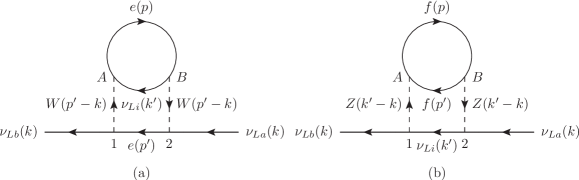
Figure 1: Two-loop diagrams for the damping term in the neutrino thermal self-energy in a matter (electron and nucleon) background. In Diagram (b) the label $f$ stands for either $e,n,p$. In principle we have to consider the various thermal vertices $A=1,2$ and $B=1,2$. However, in the heavy $W,Z$ limit, only the diagonal components of the $W,Z$ thermal propagators are non-zero and therefore only one diagram, with $A=1$ and $B=2$, must be considered. For simplicity of notation, we have labeled $k^{\prime}=p-p^{\prime}+k$.

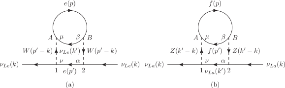
Figure 2: Same diagrams as in Fig. 1 but restricted to the case of standard neutrino couplings in the standard model. In diagram (a) only $\nu_{e}$ can participate, while in diagram (b) the neutrino line labeled $\nu_{a}$ can be anyone of the flavors $\nu_{e,\mu,\tau}$, but it only contributes to the flavor-diagonal matrix element. The rest of the symbols have the same meaning as in Fig. 1.

In Section 2 we review briefly our strategy to determine the jump operators from the results of the calculation of the absorptive part of the self-energy. This material is based on our previous work[4], and we therefore limit ourselves there to state the main points omitting some details. In Section 3 we proceed to the actual calculation as outlined in Section 2. The end result is a set of formulas for the decoherence terms, expressed as integrals over the distribution functions of the background particles. In Section 4 we consider the solution to the evolution equation in the two-generation case with the decoherence terms we have obtained, making contact with the previous in which the decoherence terms are treated as phenomenological parameters. In Section 5 we evaluate explicitly the integrals involved for some specific simple cases of the background conditions, which serve as a guide to practical applications. We use those results in Section 6 to give explicit formulas for the decoherence parameters in various environments of potential interest. We give special attention to the typical conditions applicable to long baseline experiments, where the effects appear to be small, and indicative that if significant decoherence effects were to be found they would be due to non-standard contributions to the decoherence terms. Section 7 contains our conclusions and we give in two appendices some of the details of the calculations.

2 Preliminaries

2.1 Self-energy and the damping matrix

The following material is borrowed from Ref. [4], which we summarize here for completeness. We denote by $u^{\mu}$ the velocity four-vector of the background medium and by $k^{\mu}$ the momentum of the propagating neutrino. In the background medium’s own rest frame,

$$u^{\mu}=(1,\vec{0})\,,$$ (2.1)

and in this frame we also write

$$k^{\mu}=(\omega,\vec{\kappa})\,.$$ (2.2)

Since we consider only one background medium, which can be taken to be at rest, we adopt Eqs. (2.1) and (2.2) throughout.

Let us consider first the case of one neutrino propagating in the medium, ignoring flavor mixing. The dispersion relation $\omega(\vec{\kappa})$ and the spinor of the propagating mode are determined by solving the equation

$$\left(k\hbox to0.0pt{\hss/}-\Sigma_{eff}\right)\psi_{L}(k)=0\,,$$ (2.3)

where $\Sigma_{eff}$ is the neutrino thermal self-energy, which can be decomposed in the form

$$\Sigma_{eff}=\Sigma_{r}+i\Sigma_{i}\,,$$ (2.4)

where $\Sigma_{r}$ is the dispersive part and $\Sigma_{i}$ the absorptive part. In the context of thermal field theory,

$$\Sigma_{r}=\Sigma_{11r}\equiv\frac{1}{2}(\Sigma_{11}+\overline{\Sigma}_{11})\,,$$ (2.5)

where $\Sigma_{11}$ is the $11$ element of the thermal self-energy matrix. On the other hand, $\Sigma_{i}$ is conveniently obtained from the formula

$$\Sigma_{i}=\frac{\Sigma_{12}}{2in_{F}(x_{\nu})}\,,$$ (2.6)

where $\Sigma_{12}(k)$ is the $12$ element of the neutrino thermal self-energy matrix, while

$$n_{F}(z)=\frac{1}{e^{z}+1}\,,$$ (2.7)

is the fermion distribution function, written in terms of a dummy variable $z$, and the variable $x_{\nu}$ is given by

$$x_{\nu}=\beta k\cdot u-\alpha_{\nu}\,.$$ (2.8)

$\Sigma_{11}$ and $\Sigma_{12}$ will be determined by evaluating the diagrams shown in Fig. 2.

The chirality of the interactions imply that[22]

$$\Sigma_{eff}=V^{\mu}\gamma_{\mu}L\,,$$ (2.9)

and correspondingly

$$\Sigma_{r,i}=V^{\mu}_{r,i}\gamma_{\mu}L\,,$$ (2.10)

with

$$V^{\mu}=V^{\mu}_{r}+iV^{\mu}_{i}\,.$$ (2.11)

In general both $V^{\mu}_{r,i}$ are functions of $\omega$ and $\vec{\kappa}$. Ordinarily we will omit those arguments but we will restore them when needed.

Writing the neutrino and antineutrino dispersion relations in the form

$$\omega^{(\nu,\bar{\nu})}=\omega^{(\nu,\bar{\nu})}_{r}-\frac{i\gamma^{(\nu,\bar{\nu})}}{2}\,,$$ (2.12)

$\omega^{(\nu,\bar{\nu})}_{r}$ is given by

$$\omega^{(\nu,\bar{\nu})}_{r}=\kappa+V^{(\nu,\bar{\nu})}_{eff}$$ (2.13)

where $V^{(\nu,\bar{\nu})}_{eff}$ are the effective potentials

$$V^{(\nu)}_{eff} = n\cdot V_{r}(\kappa,\vec{\kappa})=V^{0}_{r}(\kappa,\vec{\kappa})-\hat{\kappa}\cdot\vec{V}_{r}(\kappa,\vec{\kappa})\,,$$

$$V^{(\bar{\nu})}_{eff} = -n\cdot V_{r}(-\kappa,-\vec{\kappa})=-V^{0}_{r}(-\kappa,-\vec{\kappa})+\hat{\kappa}\cdot\vec{V}_{r}(-\kappa,-\vec{\kappa})\,,$$ (2.14)

with

$$n^{\mu}=(1,\hat{\kappa})\,.$$ (2.15)

On the other hand, for the imaginary part,

$$-\frac{\gamma^{(\nu)}(\vec{\kappa})}{2} = \frac{n\cdot V_{i}(\kappa,\vec{\kappa})}{1-n\cdot\left.\frac{\partial V_{r}(\omega,\vec{\kappa})}{\partial\omega}\right|_{\omega=\kappa}}\,,$$

$$-\frac{\gamma^{(\bar{\nu})}(\vec{\kappa})}{2} = \frac{n\cdot V_{i}(-\kappa,-\vec{\kappa})}{1-n\cdot\left.\frac{\partial V_{r}(\omega,-\vec{\kappa})}{\partial\omega}\right|_{\omega=-\kappa}}\,,$$ (2.16)

where $n^{\mu}$ is defined in Eq. (2.15). If the correction due to the $n\cdot\partial V_{r}(\omega,\vec{\kappa})/\partial\omega$ in the denominator can be neglected, the formulas in Eq. (2.1) reduce to

$$-\frac{\gamma^{(\nu)}(\vec{\kappa})}{2} = n\cdot V_{i}(\kappa,\vec{\kappa})\,,$$

$$-\frac{\gamma^{(\bar{\nu})}(\vec{\kappa})}{2} = n\cdot V_{i}(-\kappa,-\vec{\kappa})\,.$$ (2.17)

When we consider various neutrino flavors, the vector $V^{\mu}$ defined through Eq. (2.9) is a matrix in neutrino flavor space. Then, as shown in Ref. [4], generalization of the discussion above is that the dispersion relations of the propagating modes are determined by solving the following eigenvalue equation, in flavor-space,

$$\left(H_{r}-i\frac{\Gamma}{2}\right)\xi=\omega\xi\,,$$ (2.18)

with $H_{r}$ and $\Gamma$ being Hermitian matrices in flavor space, calculated in terms of the vector $V_{\mu}$,

$$H_{r} = \left\{\begin{array}[]{ll}\kappa+n\cdot V_{r}(\kappa,\vec{\kappa})&(\nu)\\ \kappa-n\cdot V^{\ast}_{r}(-\kappa,-\vec{\kappa})&(\bar{\nu})\end{array}\right.$$ (2.21)

$$-\frac{1}{2}\Gamma = \left\{\begin{array}[]{ll}n\cdot V_{i}(\kappa,\vec{\kappa})&(\nu)\\ n\cdot V^{\ast}_{i}(-\kappa,-\vec{\kappa})&(\bar{\nu})\end{array}\right.\,.$$ (2.24)

In coordinate space, this translates to the evolution equation

$$i\partial_{t}\xi(t)=\left(H_{r}-i\frac{\Gamma}{2}\right)\xi(t)\,.$$ (2.25)

Our purpose is to determine the contribution to $\Gamma$ due to the diagrams in Fig. 2. Our strategy is first to determine the loop-expression for $\Sigma_{i}$, which follows from the corresponding loop-expression for $\Sigma_{12}$ by means of Eq. (2.6). Then use the fact that the corresponding expression for $V^{\mu}_{i}$ is obtained by substituting the loop-expression for $\Sigma_{i}$ in the formula

$$V^{\mu}_{i}=\frac{1}{2}\mbox{Tr}\,\gamma^{\mu}\Sigma_{i}\,,$$ (2.26)

as implied by Eq. (2.10), which allows to calculate $\Gamma$ by means of Eq. (2.21). Specifically, we will denote by $\Sigma^{(W)}_{i}$ the contribution from diagram (a)in Fig. 2 and by $\Sigma^{(Z,f)}_{i}$ the contribution from diagram (b) for any of the fermions $f=e,n,p$, so that

$$\Sigma_{i}=\Sigma^{(W)}_{i}+\sum_{f=e,n,p}\Sigma^{(Z,f)}_{i}\,.$$ (2.27)

From Eqs. (2.21) and (2.26) we then obtain the loop formula for the damping matrix

$$-\frac{1}{2}\Gamma^{(\nu)} = n\cdot V^{(W)}_{i}(\kappa,\vec{\kappa})+\sum_{f=e,n,p}n\cdot V^{(Z,f)}_{i}(\kappa,\vec{\kappa})\,,$$

$$-\frac{1}{2}\Gamma^{(\bar{\nu})} = n\cdot V^{(W)\ast}_{i}(-\kappa,-\vec{\kappa})+\sum_{f=e,n,p}n\cdot V^{(Z,f)\ast}_{i}(-\kappa,-\vec{\kappa})\,.$$ (2.28)

for neutrinos and antineutrinos, respectively, where

$$V^{(Z,f)\alpha}_{i} = \frac{1}{2}\mbox{Tr}\,\gamma^{\alpha}\Sigma^{(Z,f)}_{i}\,,$$

$$V^{(W)\alpha}_{i} = \frac{1}{2}\mbox{Tr}\,\gamma^{\alpha}\Sigma^{(W)}_{i}\,,$$ (2.29)

2.2 Jump operators

Similarly to the case discussed in Ref. [4], the damping matrix in the present case, calculated from Fig. 2 as we have outlined above, arises from the non-forward neutrino scattering processes, and not from neutrino decay processes. In this case the initial neutrino state is depleted but does not actually disappear and, as we argued, the damping matrix should be associated with decoherence effects in terms of the Lindblad equation and the notion of the stochastic evolution of the state vector[5, 6, 7, 8, 9]. The idea is to assume that the evolution due to the damping effects described by $\Gamma$ is accompanied by a stochastic evolution that cannot be described by the coherent evolution of the state vector. As discussed in detail in Ref. [4] but omitting the details here, the result of this idea is that the evolution of the system in this case is described by the density matrix (in the sense that we can use it to calculate averages of quantum expectation values) that satisfies the Lindblad equation,

$$\partial_{t}\rho=-i[H_{r},\rho]+\sum_{n}\left\{L_{n}\rho L^{\dagger}_{n}-\frac{1}{2}L^{\dagger}_{n}L_{n}\rho-\frac{1}{2}\rho L^{\dagger}_{n}L_{n}\right\}\,,$$ (2.30)

where the $L_{n}$ matrices, representing the jump operators, are related to $\Gamma$ by

$$\Gamma=\sum_{n}L^{\dagger}_{n}L_{n}\,.$$ (2.31)

Indeed, as we will show, the damping matrix that we will determine by means of Eq. (2.1), can be written in the form

$$\Gamma=L^{(W)\dagger}_{e}L^{(W)}_{e}+\sum_{f=e,n,p}L^{(Z)\dagger}_{f}L^{(Z)}_{f}\,,$$ (2.32)

with well-defined expressions for the $L$ matrices in terms of integrals over the background particles distribution functions that we will obtain from the self-energy calculation.

2.3 Notation and conventions

For definiteness we state precisely the notation and conventions we use throughout. The neutral-current couplings of the interaction Lagrangian that are relevant to our calculation are given by

$$L_{Z}=-g_{Z}Z^{\mu}\left[\sum_{a}\overline{\nu}_{La}\gamma_{\mu}\nu_{La}+\overline{e}\gamma_{\mu}(a_{e}+b_{e}\gamma_{5})e+J^{(Z)}_{\mu}\right]\,,$$ (2.33)

where, in the standard model,

$$g_{Z}=g/(2\cos\theta_{W})$$ (2.34)

and

$$a_{e} = -\frac{1}{2}+2\sin^{2}\theta_{W}\,,$$

$$b_{e} = \frac{1}{2}\,.$$ (2.35)

On the other hand, $J^{(Z)}_{\mu}$ is the nucleon neutral current, which in terms of the quark fields

$$q=\left(\begin{array}[]{l}u\\ d\end{array}\right)\,,$$ (2.36)

is given by

$$J^{(Z)}_{\mu}=\overline{q}\gamma_{\mu}\frac{\tau_{3}}{2}q-\overline{q}\gamma_{\mu}\gamma_{5}\frac{\tau_{3}}{2}q-2\sin^{2}\theta_{W}J^{(em)}_{\mu}\,,$$ (2.37)

where $J^{(em)}_{\mu}$ is the electromagnetic current

$$J^{(em)}_{\mu}=\overline{q}\gamma_{\mu}\frac{\tau_{3}}{2}q+\frac{1}{6}\overline{q}\gamma_{\mu}q\,,$$ (2.38)

and $\tau_{1,2,3}$ stand for the Pauli matrices.

We introduce the nucleon ($f=n,p$) neutral-current vertex function $j^{(Z)}_{f\mu}(q)$, which is defined such that the matrix element of the neutral-current between nucleon states is given by

$$\langle f(p^{\prime})|J^{(Z)}_{\mu}(0)|f(p)\rangle=\overline{u}(p^{\prime})j^{(Z)}_{f\mu}(p-p^{\prime})u(p)\,.$$ (2.39)

We parametrize $j^{(Z)}_{f\mu}(q)$ in the form

$$j^{(Z)}_{f\mu}(q)=a_{f}\gamma_{\mu}+b_{f}\gamma_{\mu}\gamma_{5}-i\frac{c_{f}}{2m_{N}}\sigma_{\mu\nu}q^{\nu}\,.$$ (2.40)

In principle the parameters $a_{f},b_{f},c_{f}$ are $q^{2}$-dependent form factors. For our purposes we will assume that it is valid to adopt their $q^{2}=0$ limiting value. In this case,

$$a_{f} = I_{3f}-2\sin^{2}\theta_{W}Q_{f}\,,$$

$$b_{f} = -I_{3f}g_{A}\,,$$

$$c_{f} = I_{3f}[F^{(em)}_{2p}(0)-F^{(em)}_{2n}(0)]-2\sin^{2}\theta_{W}F^{(em)}_{2f}(0)\,,$$ (2.41)

where $Q_{p}=1,Q_{n}=0$, $I_{3p}=-I_{3n}=1/2$ and

$$F_{2p}^{(em)}(0) = 1.79\,,$$

$$F_{2n}^{(em)}(0) = -1.71\,.$$ (2.42)

In addition we will discard the $c_{f}$ term since it contains a factor of $q/m_{N}$ which gives a small contribution relative to the other terms. For the charged current,

$$L_{W}=-\left(\frac{g}{\sqrt{2}}\right)W^{\mu}\nu_{L}\gamma_{\mu}e_{L}+h.c.$$ (2.43)

3 Calculation of $\Gamma$ and the jump operators

3.1 Calculation of $\Sigma_{12}$

We consider first the contribution to $\Sigma_{12}(k)$ from diagram (b) in Fig. 2. In the heavy $Z$ limit, only the diagonal elements of the $Z$ propagator are non-zero, $\Delta^{(Z)}_{22\mu\nu}=-\Delta^{(Z)}_{11\mu\nu}=-g_{\mu\nu}/m^{2}_{Z}$, and therefore only the terms with $A=1,B=2$ contribute. Each fermion in the background contributes a term that we write in the form

$$-i\left(\Sigma^{(Z,f)}_{12}(k)\right)_{ba} = -2K^{(Z)}_{ba}\int\frac{d^{4}p^{\prime}}{(2\pi)^{4}}\frac{d^{4}p}{(2\pi)^{4}}\gamma^{\mu}LiS^{(\nu_{La})}_{12}(k^{\prime})\gamma^{\nu}L$$ (3.1)

$$\mbox{}\times\mbox{Tr}\,\left(\gamma_{\mu}(a_{f}+b_{f}\gamma_{5})iS^{(f)}_{12}(p^{\prime})\gamma_{\nu}(a_{f}+b_{f}\gamma_{5})iS^{(f)}_{21}(p)\right)\,,$$

where

$$K^{(Z)}_{ba}=\left(\frac{g^{4}_{Z}}{2m^{4}_{Z}}\right)\delta_{ab}=\left(\frac{g^{4}}{32m^{4}_{W}}\right)\delta_{ab}\,,$$ (3.2)

and

$$k^{\prime}\equiv p-p^{\prime}+k\,.$$ (3.3)

The corresponding expression for the contribution from diagram (a) can be obtained from Eq. (3.1) by making simple substitutions. Thus,

$$-i\left(\Sigma^{(W)}_{12}(k)\right)_{ba} = -2K^{(W)}_{ba}\int\frac{d^{4}p^{\prime}}{(2\pi)^{4}}\frac{d^{4}p}{(2\pi)^{4}}\gamma^{\mu}LiS^{(e)}_{12}(p^{\prime})\gamma^{\nu}L$$ (3.4)

$$\mbox{}\times\mbox{Tr}\,\left(\gamma_{\mu}LiS^{(\nu_{Le})}_{12}(k^{\prime})\gamma_{\nu}LiS^{(e)}_{21}(p)\right)\,,$$

where

$$K^{(W)}_{ba}=\left(\frac{g^{4}}{8m^{4}_{W}}\right)\delta_{ae}\delta_{be}\,,$$ (3.5)

which can in turn be rewritten in the form (the proof is given in Appendix A)

$$-i\left(\Sigma^{(W)}_{12}(k)\right)_{ba} = -2K^{(W)}_{ba}\int\frac{d^{4}p^{\prime}}{(2\pi)^{4}}\frac{d^{4}p}{(2\pi)^{4}}\gamma^{\mu}LiS^{(\nu_{Le})}_{12}(k^{\prime})\gamma^{\nu}L$$ (3.6)

$$\mbox{}\times\mbox{Tr}\,\left(\gamma_{\mu}LiS^{(e)}_{12}(p^{\prime})\gamma_{\nu}LiS^{(e)}_{21}(p)\right)\,.$$

Therefore, in what follows we concentrate on the evaluation of $\Sigma^{(Z,f)}_{12}(k)$ using Eq. (3.1). The results for $\Sigma^{(W)}_{12}(k)$ are obtained by making the replacements

$$K^{(Z)}_{ba} \rightarrow K^{(W)}_{ba}\,,$$

$$a_{e}=-b_{e} \rightarrow \frac{1}{2}\,,$$ (3.7)

in the results for $\Sigma^{(Z,e)}_{12}(k)$.

For the propagators of the internal fermion and neutrino lines we adopt the same formulas used in Ref. [4]. Specifically, we express the components of the $f$ propagator matrices in the form

$$S^{(f)}_{21}(p) = -2\pi i\delta(p^{2}-m^{2}_{f})\sigma^{(f)}(p)e^{x_{f}}n_{F}(x_{f})\epsilon(p\cdot u)\,,$$

$$S^{(f)}_{12}(p^{\prime}) = 2\pi i\delta(p^{\prime\,2}-m^{2}_{f})\sigma^{(f)}(p^{\prime})n_{F}(x^{\prime}_{f})\epsilon(p^{\prime}\cdot u)\,,$$ (3.8)

where

$$\sigma^{(f)}(q)=q\hbox to0.0pt{\hss/}+m_{f}\,,$$ (3.9)

$n_{F}(z)$ is the fermion distribution function defined in Eq. (2.7), $\epsilon(z)=\theta(z)-\theta(-z)$ where $\theta(z)$ is the step function, and we have defined

$$x_{f} = \beta p\cdot u-\alpha_{f}\,,$$

$$x^{\prime}_{f} = \beta p^{\prime}\cdot u-\alpha_{f}\,.$$ (3.10)

For the neutrino propagator, we neglect the effect of the non-zero neutrino masses and/or dispersion relations in the calculation of $\Sigma_{12}$ as in Ref. [4]. In this case the neutrino propagator is diagonal in flavor space, with all the elements actually being the same since all the neutrinos have the same mass (zero) and the same chemical potential. Specifically,

$$(S^{(\nu_{La})}_{12}(k^{\prime}))=2\pi i\delta(k^{\prime\,2})\sigma^{(\nu)}(k^{\prime})n_{F}(x^{\prime}_{\nu})\epsilon(k^{\prime}\cdot u)\,,$$ (3.11)

where

$$x^{\prime}_{\nu}=\beta k^{\prime}\cdot u-\alpha_{\nu}\,,$$ (3.12)

and

$$\sigma^{(\nu)}(k^{\prime})=Lk\hbox to0.0pt{\hss/}^{\prime}\,.$$ (3.13)

The distribution function for the fermion $f$ and neutrino are denoted by $f_{f}$ and $f_{\nu}$, respectively, with

$$f_{f}(\epsilon)=\frac{1}{e^{\beta\epsilon-\alpha_{f}}+1}\,,$$ (3.14)

and an analogous formula for $f_{\nu}$, while corresponding formulas for the antiparticles, $f_{\bar{f},\bar{\nu}}$, are given by reversing the sign of $\alpha_{f,\nu}$.

We will denote by $\Sigma^{(Z,f)}_{i}$ the contribution to $\Sigma_{i}$ due to the $\Sigma^{(Z,f)}_{12}$ term we are considering. That is, from Eq. (2.6),

$$\Sigma^{(Z,f)}_{i}(k)=\frac{\Sigma^{(Z,f)}_{12}}{2in_{F}(x_{\nu})}\,.$$ (3.15)

In the following steps we mimic the procedure we used in Ref. [4], and therefore we omit here some of the details. Thus, we let $k^{\prime}$ be an arbitrary four-momentum variable in the integral expression for $\Sigma^{(Z,f)}_{12}$ but insert the factor $\delta^{(4)}(k^{\prime}+p^{\prime}-p-k)$ and integrating over $k^{\prime}$. Then carrying out the integral over $k^{\prime\,0}$, with the help of the delta function,

$$\left(\Sigma^{(Z,f)}_{i}(k)\right)_{ba} = -K^{(Z)}_{ba}\int\frac{d^{4}p^{\prime}}{(2\pi)^{3}}\frac{d^{4}p}{(2\pi)^{3}}\frac{d^{3}\kappa^{\prime}}{(2\pi)^{3}2\omega_{\kappa^{\prime}}}\delta(p^{\prime\,2}-m^{2}_{f})\delta(p^{2}-m^{2}_{f})\epsilon(p\cdot u)\epsilon(p^{\prime}\cdot u)$$ (3.16)

$$\times(2\pi)^{4}\left\{\delta^{(4)}(k+p-k^{\prime}-p^{\prime})N_{\mu\nu}(p,p^{\prime})M^{\mu\nu}(k^{\prime})E_{\nu}\right.$$

$$-\left.\delta^{(4)}(k+p+k^{\prime}-p^{\prime})N_{\mu\nu}(p,p^{\prime})M^{\mu\nu}(-k^{\prime})E_{\bar{\nu}}\right\}\,,$$

where

$$M^{\mu\nu}(k^{\prime}) = \gamma^{\mu}L\sigma^{(\nu)}(k^{\prime})\gamma^{\nu}L\,,$$

$$N_{\mu\nu}(p,p^{\prime}) = \mbox{Tr}\,\left(\gamma_{\mu}(a_{f}+b_{f}\gamma_{5})\sigma^{(f)}(p^{\prime})\gamma_{\nu}(a_{f}+b_{f}\gamma_{5})\sigma^{(f)}(p)\right)\,,$$ (3.17)

and

$$E_{\nu} = n_{F}(x_{f})(1-n_{F}(x^{\prime}_{f}))-f_{\nu}(\omega_{\kappa^{\prime}})(n_{F}(x_{f})-n_{F}(x^{\prime}_{f}))\,,$$

$$E_{\bar{\nu}} = n_{F}(x^{\prime}_{f})(1-n_{F}(x_{f}))+f_{\bar{\nu}}(\omega_{\kappa^{\prime}})(n_{F}(x_{f})-n_{F}(x^{\prime}_{f}))\,,$$ (3.18)

with

$$k^{\prime\,\mu} = (\omega_{\kappa^{\prime}},\vec{\kappa}^{\prime})\,,$$

$$\omega_{\kappa^{\prime}} = |\vec{\kappa}^{\prime}|\,.$$ (3.19)

Next carrying out the integration over $p^{0},p^{\prime\,0}$ in a similar way, we obtain

$$\left(\Sigma^{(Z,f)}_{i}(k)\right)_{ba} = -K^{(Z)}_{ba}\int\frac{d^{3}p^{\prime}}{(2\pi)^{3}2E_{p^{\prime}}}\frac{d^{3}p}{(2\pi)^{3}2E_{p}}\frac{d^{3}\kappa^{\prime}}{(2\pi)^{3}2\omega_{\kappa^{\prime}}}$$ (3.20)

$$\times(2\pi)^{4}\left\{\delta^{(4)}(k+p-k^{\prime}-p^{\prime})N_{\mu\nu}(p,p^{\prime})M^{\mu\nu}(k^{\prime})E_{\nu,++}\right.$$

$$-\left.\delta^{(4)}(k-p-k^{\prime}-p^{\prime})N_{\mu\nu}(-p,p^{\prime})M^{\mu\nu}(k^{\prime})E_{\nu,-+}\right.$$

$$-\left.\delta^{(4)}(k+p+p^{\prime}-k^{\prime})N_{\mu\nu}(p,-p^{\prime})M^{\mu\nu}(k^{\prime})E_{\nu,+-}\right.$$

$$+\left.\delta^{(4)}(k+p^{\prime}-k^{\prime}-p)N_{\mu\nu}(-p,-p^{\prime})M^{\mu\nu}(k^{\prime})E_{\nu,--}\right.$$

$$-\left.\delta^{(4)}(k+p+k^{\prime}-p^{\prime})N_{\mu\nu}(p,p^{\prime})M^{\mu\nu}(-k^{\prime})E_{\bar{\nu},++}\right.$$

$$+\left.\delta^{(4)}(k+k^{\prime}-p^{\prime}-p)N_{\mu\nu}(-p,p^{\prime})M^{\mu\nu}(-k^{\prime})E_{\bar{\nu},-+}\right.$$

$$+\left.\delta^{(4)}(k+p+p^{\prime}+k^{\prime})N_{\mu\nu}(p,-p^{\prime})M^{\mu\nu}(-k^{\prime})E_{\bar{\nu},+-}\right.$$

$$-\left.\delta^{(4)}(k+p^{\prime}+k^{\prime}-p)N_{\mu\nu}(-p,-p^{\prime})M^{\mu\nu}(-k^{\prime})E_{\bar{\nu},--}\right\}\,,$$

with

$$p^{\mu}=(E_{p},\vec{p})\,,\qquad E_{p}=\sqrt{{\vec{p}}^{\;2}+m^{2}_{f}}\,,$$ (3.21)

and similarly for $p^{\prime\,\mu}$. In Eq. (3.20) we have introduced the factors $E_{\nu,\lambda\lambda^{\prime}}$ and $E_{\bar{\nu},\lambda\lambda^{\prime}}$ (with $\lambda,\lambda^{\prime}$ being $\pm$), which are defined as follows,

$$E_{\nu,\lambda\lambda^{\prime}}=\left.E_{\nu}\right|_{p^{0}=\lambda E_{p},\,p^{\prime\,0}=\lambda^{\prime}E_{p^{\prime}}}\,,$$ (3.22)

and similarly for $E_{\bar{\nu},\lambda\lambda^{\prime}}$. The explicit formulas are given in Table 1.

$E_{\nu,++}=f(1-f^{\prime})-f^{\prime}_{\nu}(f-f^{\prime})$	$\nu_{a}(k)+f(p)\leftrightarrow\nu_{a}(k^{\prime})+f(p^{\prime})$
$E_{\nu,-+}=(1-\bar{f})(1-f^{\prime})-f^{\prime}_{\nu}(1-\bar{f}-f^{\prime})$	$\nu_{a}(k)\leftrightarrow\nu_{a}(k^{\prime})+\bar{f}(p)+f(p^{\prime})$
$E_{\nu,+-}=f\bar{f}^{\prime}-f^{\prime}_{\nu}(f+\bar{f}^{\prime}-1)$	$\nu_{a}(k)+f(p)+\bar{f}(p^{\prime})\leftrightarrow\nu_{a}(k^{\prime})$
$E_{\nu,--}=(1-\bar{f})\bar{f}^{\prime}-f^{\prime}_{\nu}(\bar{f}^{\prime}-\bar{f})$	$\nu_{a}(k)+\bar{f}(p^{\prime})\leftrightarrow\nu_{a}(k^{\prime})+\bar{f}(p)$
$E_{\bar{\nu},++}=(1-f)f^{\prime}+\bar{f}^{\prime}_{\nu}(f-f^{\prime})$	$\nu_{a}(k)+\bar{\nu}_{a}(\bar{k}^{\prime})+f(p)\leftrightarrow f(p^{\prime})$
$E_{\bar{\nu},-+}=\bar{f}f^{\prime}+\bar{f}^{\prime}_{\nu}(1-\bar{f}-f^{\prime})$	$\nu_{a}(k)+\bar{\nu}_{a}(\bar{k}^{\prime})\leftrightarrow\bar{f}(p)+f(p^{\prime})$
$E_{\bar{\nu},+-}=(1-f)(1-\bar{f}^{\prime})+\bar{f}^{\prime}_{\nu}(f+\bar{f}^{\prime}-1)$	$\nu_{a}(k)+\bar{\nu}_{a}(\bar{k}^{\prime})+f(p)+\bar{f}(p^{\prime})\leftrightarrow 0$
$E_{\bar{\nu},--}=\bar{f}(1-\bar{f}^{\prime})+\bar{f}^{\prime}_{\nu}(\bar{f}^{\prime}-\bar{f})$	$\nu_{a}(k)+\bar{\nu}_{a}(\bar{k}^{\prime})+\bar{f}(p^{\prime})\leftrightarrow\bar{f}(p)$

Table 1: Correspondence between the $E_{\nu,\lambda\lambda^{\prime}}$ and $E_{\bar{\nu},\lambda\lambda^{\prime}}$ factors defined in Eq. (3.1), and the process that contributes to the $\nu(k)$ damping via Eq. (3.16). To simplify the notation we are using the shorthands shown in Eq. (3.1) for the various distribution functions.

To simplify the notation in the formulas summarized in Table 1 we have introduce the shorthands

$$f=f_{f}(E_{p}),\quad f^{\prime}=f_{f}(E_{p^{\prime}}),\quad f^{\prime}_{\nu}={f_{\nu}(\omega_{\kappa^{\prime}})}$$

$$\bar{f}=f_{\bar{f}}(E_{p}),\quad\bar{f}^{\prime}=f_{\bar{f}}(E_{p^{\prime}}),\quad\bar{f}^{\prime}_{\nu}=f_{\bar{\nu}}(\omega_{\kappa^{\prime}})\,.$$ (3.23)

The formulas for $E_{\bar{\nu},\lambda\lambda^{\prime}}$ are obtained from those for $E_{\nu,\lambda\lambda^{\prime}}$ by making the replacement $f^{\prime}_{\nu}\rightarrow(1-\bar{f}^{\prime}_{\nu})$.

As discussed in Ref. [4], each of the terms that appear within the bracket in Eq. (3.20) corresponds to a particular non-forward scattering process, and its inverse, for example

$$\nu_{a}(k)+f(p)\leftrightarrow\nu_{a}(k^{\prime})+f(p^{\prime})\,,$$ (3.24)

as well as the processes obtained by crossing $f(p),f(p^{\prime}),\nu_{a}(k^{\prime})$. For $\omega>0$, the only processes that are kinematically accessible are the one shown above, and the following one,

$$\nu_{a}(k)+\bar{f}(p^{\prime})\rightarrow\nu_{a}(k^{\prime})+\bar{f}(p)\,.$$ (3.25)

These correspond to the the first and the fourth terms, respectively, in the list of terms that appear within the bracket in Eq. (3.20). Alternatively, for $\omega<0$, the only kinematically accessible processes are

$$\bar{\nu}_{a}(k)+f(p^{\prime}) \rightarrow \bar{\nu}_{a}(k^{\prime})+f(p)\,,$$

$$\bar{\nu}_{a}(k)+\bar{f}(p) \rightarrow \bar{\nu}_{a}(k^{\prime})+\bar{f}(p^{\prime})\,,$$ (3.26)

which correspond to the fifth and eighth terms within the bracket in Eq. (3.20). In addition we will assume that there are no neutrinos or antineutrinos in the background, therefore we set $f_{\nu}$ and $f_{\bar{\nu}}$ to zero. Then,

$$\left(\Sigma^{(Z,f)}_{i}(k)\right)_{ba} = -K^{(Z)}_{ba}\int\frac{d^{3}p^{\prime}}{(2\pi)^{3}2E_{p^{\prime}}}\frac{d^{3}p}{(2\pi)^{3}2E_{p}}\frac{d^{3}\kappa^{\prime}}{(2\pi)^{3}2\omega_{\kappa^{\prime}}}$$

$$\times(2\pi)^{4}\left\{\delta^{(4)}(k+p-k^{\prime}-p^{\prime})N_{\mu\nu}(p,p^{\prime})M^{\mu\nu}(k^{\prime})\left[f_{f}(E_{p})(1-f_{f}(E_{p^{\prime}}))\right]\right.$$

$$+\left.\delta^{(4)}(k+p^{\prime}-k^{\prime}-p)N_{\mu\nu}(-p,-p^{\prime})M^{\mu\nu}(k^{\prime})\left[(1-f_{\bar{f}}(E_{p}))f_{\bar{f}}(E_{p^{\prime}})\right]\right\}\,.$$

$$+\left.\delta^{(4)}(k+p+k^{\prime}-p^{\prime})N_{\mu\nu}(p,p^{\prime})M^{\mu\nu}(k^{\prime})\left[(1-f_{f}(E_{p}))f_{f}(E_{p^{\prime}})\right]\right.$$

$$+\left.\delta^{(4)}(k+p^{\prime}+k^{\prime}-p)N_{\mu\nu}(-p,-p^{\prime})M^{\mu\nu}(k^{\prime})\left[f_{\bar{f}}(E_{p})(1-f_{\bar{f}}(E_{p^{\prime}}))\right]\right\}\,,$$

where we have used the fact that $M^{\mu\nu}(-k^{\prime})=-M^{\mu\nu}(k^{\prime})$ and, as we have mentioned, if $\omega>0$ only the first two terms in the bracket contribute, while for $\omega<0$ only the last two contribute.

3.2 Calculation of $n\cdot V_{i}$

As already stated in Section 2, the contribution to $\left(V^{\alpha}_{i}(\omega,\vec{\kappa})\right)_{ba}$, which we denote by $\left(V^{(Z,f)\alpha}_{i}(\omega,\vec{\kappa})\right)_{ba}$, is obtained by substituting Eq. (3.1) in Eq. (2.1). It then follows that the formula for $\left(V^{(Z,f)\alpha}_{i}(\omega,\vec{\kappa})\right)_{ba}$ is obtained from Eq. (3.1) by making the replacement

$$M^{\mu\nu}(k^{\prime})\rightarrow L^{\alpha\mu\nu}(k^{\prime})\,.$$ (3.28)

where

$$L^{\alpha\mu\nu}(k^{\prime}) \equiv \frac{1}{2}\mbox{Tr}\,\gamma^{\alpha}M^{\mu\nu}(k^{\prime})$$ (3.29)

$$= \frac{1}{2}\mbox{Tr}\,\gamma^{\alpha}\gamma^{\mu}L\sigma^{(\nu)}(k^{\prime})\gamma^{\nu}L$$

$$= \frac{1}{2}\mbox{Tr}\,L\gamma^{\alpha}\gamma^{\mu}k\hbox to0.0pt{\hss/}^{\prime}\gamma^{\nu}\,.$$

That is,

$$\left(V^{(Z,f)\alpha}_{i}(\omega,\vec{\kappa})\right)_{ba} = -K^{(Z)}_{ba}\int\frac{d^{3}p^{\prime}}{(2\pi)^{3}2E_{p^{\prime}}}\frac{d^{3}p}{(2\pi)^{3}2E_{p}}\frac{d^{3}\kappa^{\prime}}{(2\pi)^{3}2\omega_{\kappa^{\prime}}}$$ (3.30)

$$\times(2\pi)^{4}\left\{\delta^{(4)}(k+p-k^{\prime}-p^{\prime})N_{\mu\nu}(p,p^{\prime})L^{\alpha\mu\nu}(k^{\prime})\left[f_{f}(E_{p})(1-f_{f}(E_{p^{\prime}}))\right]\right.$$

$$+\left.\delta^{(4)}(k+p^{\prime}-k^{\prime}-p)N_{\mu\nu}(-p,-p^{\prime})L^{\alpha\mu\nu}(k^{\prime})\left[(1-f_{\bar{f}}(E_{p}))f_{\bar{f}}(E_{p^{\prime}})\right]\right.$$

$$+\left.\delta^{(4)}(k+p+k^{\prime}-p^{\prime})N_{\mu\nu}(p,p^{\prime})L^{\alpha\mu\nu}(k^{\prime})\left[(1-f_{f}(E_{p}))f_{f}(E_{p^{\prime}})\right]\right.$$

$$+\left.\delta^{(4)}(k+p^{\prime}+k^{\prime}-p)N_{\mu\nu}(-p,-p^{\prime})L^{\alpha\mu\nu}(k^{\prime})\left[f_{\bar{f}}(E_{p})(1-f_{\bar{f}}(E_{p^{\prime}}))\right]\right\}\,.$$

The traces involved in Eqs. (3.1) and (3.29) are easily evaluated by means of the standard formulas. After some straightforward algebra, this procedure leads to

$$\left(V^{(Z,f)\alpha}_{i}(\omega,\vec{\kappa})\right)_{ba} = -8K^{(Z)}_{ba}\int\frac{d^{3}p^{\prime}}{(2\pi)^{3}2E_{p^{\prime}}}\frac{d^{3}p}{(2\pi)^{3}2E_{p}}\frac{d^{3}\kappa^{\prime}}{(2\pi)^{3}2\omega_{\kappa^{\prime}}}v^{\alpha}(k^{\prime},p,p^{\prime})$$ (3.31)

$$\times(2\pi)^{4}\left\{\delta^{(4)}(k+p-k^{\prime}-p^{\prime})\left[f_{f}(E_{p})(1-f_{f}(E_{p^{\prime}}))\right]\right.$$

$$+\left.\delta^{(4)}(k+p^{\prime}-k^{\prime}-p)\left[(1-f_{\bar{f}}(E_{p}))f_{\bar{f}}(E_{p^{\prime}})\right]\right\}\,.$$

$$+\left.\delta^{(4)}(k+p+k^{\prime}-p^{\prime})\left[(1-f_{f}(E_{p}))f_{f}(E_{p^{\prime}})\right]\right.$$

$$+\left.\delta^{(4)}(k+p^{\prime}+k^{\prime}-p)\left[f_{\bar{f}}(E_{p})(1-f_{\bar{f}}(E_{p^{\prime}}))\right]\right\}\,,$$

where

$$v^{\alpha}(k^{\prime},p,p^{\prime})\equiv-m^{2}_{f}(a^{2}_{f}-b^{2}_{f})k^{\prime\,\alpha}+(a_{f}-b_{f})^{2}(k^{\prime}\cdot p^{\prime})p^{\alpha}+(a_{f}+b_{f})^{2}(k^{\prime}\cdot p)p^{\prime\,\alpha}\,.$$ (3.32)

The quantities that enter in the formula for $\Gamma$ are then,

$$n\cdot\left(V^{(Z,f)}_{i}(\kappa,\vec{\kappa})\right)_{ba} = -4K^{(Z)}_{ba}\left\{-m^{2}_{f}(a^{2}_{f}-b^{2}_{f})(I^{(f)}_{0}+I^{(\bar{f})}_{0})\right.$$ (3.33)

$$\mbox{}+\left.(a_{f}+b_{f})^{2}(I^{(f)}_{1}+I^{(\bar{f})}_{2})\right.$$

$$\mbox{}+\left.(a_{f}-b_{f})^{2}(I^{(f)}_{2}+I^{(\bar{f})}_{1})\right\}\,,$$

$$n\cdot\left(V^{(Z,f)}_{i}(-\kappa,-\vec{\kappa})\right)_{ba} = -4K^{(Z)}_{ba}\left\{-m^{2}_{f}(a^{2}_{f}-b^{2}_{f})(I^{(f)}_{0}+I^{(\bar{f})}_{0})\right.$$ (3.34)

$$\mbox{}+\left.(a_{f}+b_{f})^{2}(I^{(f)}_{2}+I^{(\bar{f})}_{1})\right.$$

$$\mbox{}+\left.(a_{f}-b_{f})^{2}(I^{(f)}_{1}+I^{(\bar{f})}_{2})\right\}\,,$$

where we have introduced the integrals $I^{(f,\bar{f})}_{0}$, which for either case ($x=f,\bar{f}$) is defined as

$$I^{(x)}_{0} = \frac{2}{\omega_{\kappa}}\int\frac{d^{3}\kappa^{\prime}}{(2\pi)^{3}2\omega_{\kappa^{\prime}}}\frac{d^{3}p^{\prime}}{(2\pi)^{3}2E_{p^{\prime}}}\frac{d^{3}p}{(2\pi)^{3}2E_{p}}$$ (3.35)

$$\times(2\pi)^{4}\delta^{(4)}(p+q-p^{\prime})f_{x}(E_{p})\left(1-f_{x}(E_{p^{\prime}})\right)k\cdot k^{\prime}\,,$$

while $I^{(f,\bar{f})}_{1,2}$ are the same integrals defined in Ref. [4], which we reproduce here for convenience,

$$I^{(x)}_{1} = \frac{2}{\omega_{\kappa}}\int\frac{d^{3}p}{(2\pi)^{3}2E_{p}}\frac{d^{3}p^{\prime}}{(2\pi)^{3}2E_{p^{\prime}}}\frac{d^{3}\kappa^{\prime}}{(2\pi)^{3}2\omega_{\kappa^{\prime}}}$$

$$\times(2\pi)^{4}\delta^{(4)}(p+k-p^{\prime}-k^{\prime})f_{x}(E_{p})\left(1-f_{x}(E_{p^{\prime}})\right)(p\cdot k^{\prime})^{2}\,,$$

$$I^{(x)}_{2} = \frac{2}{\omega_{\kappa}}\int\frac{d^{3}p}{(2\pi)^{3}2E_{p}}\frac{d^{3}p^{\prime}}{(2\pi)^{3}2E_{p^{\prime}}}\frac{d^{3}\kappa^{\prime}}{(2\pi)^{3}2\omega_{\kappa^{\prime}}}$$ (3.36)

$$\times(2\pi)^{4}\delta^{(4)}(p+k-p^{\prime}-k^{\prime})f_{x}(E_{p})\left(1-f_{x}(E_{p^{\prime}})\right)(p\cdot k)^{2}\,.$$

In these integral formulas, we understand that $k$ is set to

$$k^{\mu}=(\omega_{\kappa},\vec{\kappa})\,,$$ (3.37)

with $\omega_{\kappa}=\kappa$, and similarly for $k^{\prime}$.

3.3 Formula for $\Gamma$

We can now obtain the explicit formula for the damping matrix in terms of the integrals $I^{(x)}_{0,1,2}$. The damping matrix is given by Eq. (2.1), where $n\cdot V^{(Z,f)}_{i}(\kappa,\vec{\kappa})$ and $n\cdot V^{(Z,f)}_{i}(-\kappa,-\vec{\kappa})$ are given above in Eqs. (3.33) and (3.34) while the formulas for $n\cdot V^{(W)}(\kappa,\vec{\kappa})$ and $n\cdot V^{(W)}(-\kappa,-\vec{\kappa})$ are obtained from the corresponding formulas for $n\cdot V^{(Z,f)}_{i}$ by making the replacement indicated in Eq. (3.1). Therefore, for the neutrinos,

$$\Gamma^{(\nu)}_{ba}=\left(\frac{g^{2}}{2m^{2}_{W}}\right)^{2}\left[\gamma^{(W)}_{e}\delta_{be}\delta_{ae}+\left(\sum_{f}\gamma^{(Z)}_{f}\right)\delta_{ba}\right]\,,$$ (3.38)

where

$$\gamma^{(Z)}_{f} = -m^{2}_{f}(a^{2}_{f}-b^{2}_{f})(I^{(f)}_{0}+I^{(\bar{f})}_{0})+(a_{f}+b_{f})^{2}(I^{(f)}_{1}+I^{(\bar{f})}_{2})+(a_{f}-b_{f})^{2}(I^{(f)}_{2}+I^{(\bar{f})}_{1})\,,$$

$$\gamma^{(W)}_{e} = (I^{(e)}_{2}+I^{(\bar{e})}_{1})\,.$$ (3.39)

For the antineutrinos, the formula for $\Gamma^{(\bar{\nu})}$ is similar to Eq. (3.38), with $\gamma^{(W,Z)}_{f}\rightarrow\bar{\gamma}^{(W,Z)}_{f}$, where

$$\bar{\gamma}^{(Z)}_{f} = -m^{2}_{f}(a^{2}_{f}-b^{2}_{f})(I^{(f)}_{0}+I^{(\bar{f})}_{0})+(a_{f}+b_{f})^{2}(I^{(f)}_{2}+I^{(\bar{f})}_{1})+(a_{f}-b_{f})^{2}(I^{(f)}_{1}+I^{(\bar{f})}_{2})\,,$$

$$\bar{\gamma}^{(W)}_{e} = (I^{(e)}_{1}+I^{(\bar{e})}_{2})\,.$$ (3.40)

3.4 Formula for the jump operators and decoherence terms

As already explained in Section 2.2, the proposal for identifying the jump operators is based on writing $\Gamma$ as sum of terms of the form $L^{\dagger}L$. Looking at Eq. (2.1) we see that we can write $\Gamma$ in the form given in Eq. (2.32), with

$$(L^{(Z)}_{f})_{ba} = \left(\frac{g^{2}}{2m^{2}_{W}}\right)\sqrt{\gamma^{(Z)}_{f}}\delta_{ba}\,,$$

$$(L^{(W)}_{e})_{ba} = \left(\frac{g^{2}}{2m^{2}_{W}}\right)\sqrt{\gamma^{(W)}_{e}}\delta_{be}\delta_{ae}\,,$$ (3.41)

or in matrix notation,

$$L^{(Z)}_{f} = \left(\frac{g^{2}}{2m^{2}_{W}}\right)\sqrt{\gamma^{(Z)}_{f}}I\,,$$

$$L^{(W)}_{e} = \left(\frac{g^{2}}{2m^{2}_{W}}\right)\sqrt{\gamma^{(W)}_{e}}I_{e}\,,$$ (3.42)

where $I$ is the identity matrix and

$$I_{e}=\left(\begin{array}[]{ccc}1&0&0\\ 0&0&0\\ 0&0&0\end{array}\right)$$ (3.43)

For the antineutrinos, the result is similar, with $\gamma^{(W,Z)}_{f}\rightarrow\bar{\gamma}^{(W,Z)}_{f}$. Eq. (3.4), together with Eqs. (3.3) and (3.3) are the central results of the present work. We then assert that the damping effects of the non-forward scattering processes are properly taken into account in the context of the evolution equation for the flavor density matrix,

$$\partial_{t}\rho=-i[H_{r},\rho]+\sum_{\begin{subarray}{c}X=Z,W\\ f=e,n,p\end{subarray}}\left\{L^{(X)}_{f}\rho L^{(X)\dagger}_{f}-\frac{1}{2}L^{(X)\dagger}_{f}L^{(X)}_{f}\rho-\frac{1}{2}\rho L^{(X)\dagger}_{f}L^{(X)}_{f}\right\}\,,$$ (3.44)

with $L^{(W,Z)}_{f}$ given in Eq. (3.4). For reference, we refer to the terms involving the jump operators on the right-hand side of Eq. (3.44) as the decoherence terms.

Since the $L^{(Z)}_{f}$ terms are proportional to the identity matrix, they all drop out of Eq. (3.44). The evolution equation reduces to

$$\partial_{t}\rho=-i[H_{r},\rho]+D\,,$$ (3.45)

where

$$D=2\gamma\left\{I_{e}\rho I_{e}-\frac{1}{2}I_{e}\rho-\frac{1}{2}\rho I_{e}\right\}\,,$$ (3.46)

with

$$\gamma=\frac{1}{2}\left(\frac{g^{2}}{2m^{2}_{W}}\right)^{2}\gamma^{(W)}_{e}\,.$$ (3.47)

Thus, the decoherence terms are driven by $\gamma^{(W)}_{e}$ alone. However, it should be kept in mind that this result holds if all the neutrinos involved have the same neutral current couplings. In the presence of non-universality (e.g., neutrino mixing involving non-active neutrinos), the $L^{(Z)}_{f}$ terms are not proportional to the identity matrix and Eq. (3.45) does not hold. In Section 5 we evaluate the integrals required to determine $\gamma^{(W)}_{e}$ in some illustrative cases. Keeping the previous comment in mind, for completenesss we include those for $\gamma^{(Z)}_{f}$ as well.

4 Two-generation example

As an example application, for definiteness we consider the standard two-generation case in a normal matter background. The Wolfenstein term must be included in the Hamiltonian. Our discussion resembles the one in previous works that consider the decoherence effects, in which $\vec{D}$ is an unknown and treated at a phenomenological level. In those contexts the working assumption is that the decoherence terms are diagonal in the basis of the effective mass eigenstates. This is not the case with the $\vec{D}$ that we have obtained, and the question we address here is how to take into account to calculate the survival and transition probablities in the density matrix context.

We work in the flavor basis. The density matrix satisfies Eq. (3.45), with the initial normalization condition

$$\mbox{Tr}\,\rho(0)=1\,.$$ (4.1)

Up to a term proportional to identity matrix that does not contribute to the commutator, the Hamiltonian can be written in the form

$$H_{r}=\frac{1}{2}\vec{\sigma}\cdot\vec{h}\,,$$ (4.2)

with

$$\vec{h} = \left(\frac{\Delta m^{2}_{21}}{2\kappa}\sin 2\theta,\;0,\;-\frac{\Delta m^{2}_{21}}{2\kappa}\cos 2\theta+V_{e}\right)\,.$$ (4.3)

Here, $\Delta m^{2}_{21}=m^{2}_{2}-m^{2}_{1}$ and $V_{e}$ is the Wolfenstein potential for electron neutrinos $V_{e}=\sqrt{2}G_{F}n_{e}$, where $n_{e}$ is the total electron number density. It is convenient to write

$$\vec{h}=h\vec{n}\,,$$ (4.4)

where $h$ is the magnitude of $\vec{h}$,

$$h=\frac{\Delta^{2}_{m}}{2\kappa}\,,$$ (4.5)

with

$$\Delta^{2}_{m}\equiv\sqrt{(\Delta m^{2}_{21}\sin 2\theta)^{2}+(\Delta m^{2}_{21}\cos 2\theta-2\kappa V_{e})^{2}}\,,$$ (4.6)

and $\vec{n}$ is the unit vector along $\vec{h}$. We also introduce the vector with components

$$\vec{e}_{3}=(0,0,1)\,,$$ (4.7)

and define

$$\cos 2\theta_{m} = -\vec{e}_{3}\cdot\vec{n}=\frac{1}{\Delta^{2}_{m}}\left(\Delta m^{2}_{21}\cos 2\theta-2\kappa V_{e}\right)\,,$$

$$\sin^{2}2\theta_{m} = 1-(\vec{e}_{3}\cdot\vec{n})^{2}=\left(\frac{\Delta m^{2}_{21}\sin 2\theta}{\Delta^{2}_{m}}\right)^{2}\,.$$ (4.8)

Parametrizing $\rho$ in the form

$$\rho=\frac{1}{2}\left(\sigma_{0}\rho_{0}+\vec{\sigma}\cdot\vec{\rho}\right)\,,$$ (4.9)

where $\sigma_{0}$ is the unit matrix and $\vec{\sigma}$ the Pauli matrices, the evolution equation Eq. (3.45) gives

$$\partial_{t}\rho_{0} = 0\,,$$

$$\partial_{t}\vec{\rho} = h(\vec{n}\times\vec{\rho})+\vec{D}\,,$$ (4.10)

where

$$\vec{D}=-\frac{\gamma}{2}\vec{\rho}_{\perp}\,,$$ (4.11)

with

$$\vec{\rho}_{\perp}=\vec{\rho}-(\vec{e}_{3}\cdot\vec{\rho})\vec{e}_{3}\,.$$ (4.12)

Eq. (4) implies that $\rho_{0}$ is constant, and from Eq. (4.1)

$$\rho_{0}(t)=1\,.$$ (4.13)

To solve the equation for $\vec{\rho}$, let us consider briefly the equation with $\vec{D}=0$,

$$\partial_{t}\vec{\rho}=\vec{h}\times\vec{\rho}\,.$$ (4.14)

Decomposing $\rho$ into its longitudinal and transverse components to $\vec{n}$,

$$\vec{\rho}=\vec{\rho}_{\ell}+\vec{\rho}_{t}\,,$$ (4.15)

where

$$\vec{\rho}_{\ell} \equiv (\vec{n}\cdot\vec{\rho})\vec{n}\,,$$

$$\vec{\rho}_{t} \equiv \vec{\rho}-(\vec{n}\cdot\vec{\rho})\vec{n}\,,$$ (4.16)

Eq. (4.14) then implies that $\rho_{\ell}$ is constant,

$$\rho_{\ell}(t)=\rho_{\ell}(0)\,,$$ (4.17)

while for $\vec{\rho}_{t}$,

$$\partial_{t}\vec{\rho}_{t}=h\vec{n}\times\vec{\rho}_{t}\,.$$ (4.18)

This is easily solved,

$$\vec{\rho}_{t}=\cos(ht)\vec{\rho}_{t}(0)+\sin(ht)\vec{n}\times\vec{\rho}_{t}(0)\,,$$ (4.19)

so that

$$\vec{\rho}(t)=\vec{\rho}(0)+(\cos(ht)-1)\vec{\rho}_{t}(0)+\sin(ht)\vec{n}\times\vec{\rho}_{t}(0)\,,$$ (4.20)

Going back to Eq. (4.11), the point is that $\vec{\rho}_{\perp}$ mixes $\vec{\rho}_{\ell}$ and $\vec{\rho}_{t}$. In order to obtain a simple solution, albeit approximate but nevertheless useful, we will treat this mixing in a perturbative spirit. Thus we express $\vec{\rho}_{\perp}$ in the form

$$\vec{\rho}_{\perp}=a\vec{\rho}_{\ell}+b\vec{\rho}_{t}+OT\,,$$ (4.21)

where $OT$ stands for other terms that we assume can be neglected as a first approximation. Using Eq. (4), a simple calculation then yields

$$a = \sin^{2}2\theta_{m}\,,$$

$$b = \frac{1}{2}(1+\cos^{2}2\theta_{m})\,.$$ (4.22)

Within this approximation, Eqs. (4.11) and (4) give

$$\partial_{t}\vec{\rho}=h(\vec{n}\times\vec{\rho})-\gamma_{\ell}\vec{\rho}_{\ell}-\gamma_{t}\vec{\rho}_{t}\,,$$ (4.23)

or

$$\partial_{t}\rho_{\ell} = -\gamma_{\ell}\rho_{\ell}\,,$$

$$\partial_{t}\vec{\rho}_{t} = h(\vec{n}\times\vec{\rho}_{t})-\gamma_{t}\vec{\rho}_{t}\,,$$ (4.24)

where

$$\gamma_{\ell} = n^{2}_{1}\gamma=\gamma\sin^{2}2\theta_{m}\,,$$

$$\gamma_{t} = \frac{1}{2}(1+n^{2}_{3})\gamma=\frac{\gamma}{2}(1+\cos^{2}2\theta_{m})\,.$$ (4.25)

For $\rho_{\ell}(0)$ we then have

$$\rho_{\ell}(t)=e^{-\gamma_{\ell}t}\rho_{\ell}(0)\,.$$ (4.26)

A simple way to obtain the solution for $\vec{\rho}_{t}$ is to put $\vec{\rho}_{t}=e^{-\gamma_{t}t}\vec{\rho}^{\,\prime}_{t}$ , so that the equation for $\vec{\rho}^{\,\prime}_{t}$ becomes the same as the decoherence-free case. Thus we obtain

$$\vec{\rho}(t)=e^{-\gamma_{\ell}t}\vec{\rho}(0)+\left[e^{-\gamma_{t}t}\cos(ht)-e^{-\gamma_{\ell}t}\right]\vec{\rho}_{t}(0)+e^{-\gamma_{t}t}\sin(ht)\vec{n}\times\vec{\rho}_{t}(0)\,.$$ (4.27)

Of course for $\gamma_{\ell,t}=0$ we recover the decoherence-free solution Eq. (4.20).

As an example, suppose that initially

$$\rho(0)=\left(\begin{array}[]{cc}1&0\\ 0&0\end{array}\right)=\frac{1}{2}\left(1+\vec{\sigma}\cdot\vec{e}_{3}\right)\,,$$ (4.28)

which corresponds to $\vec{\rho}(0)=\vec{e}_{3}$. Then,

$$\vec{\rho}(t)=e^{-\gamma_{\ell}t}\vec{e}_{3}+\left[e^{-\gamma_{t}t}\cos(ht)-e^{-\gamma_{\ell}t}\right][\vec{e}_{3}-(\vec{n}\cdot\vec{e}_{3})\vec{n}]+e^{-\gamma_{t}t}\sin(ht)\vec{n}\times\vec{e}_{3}\,.$$ (4.29)

The survival and transition probabilities

$$P_{ee} = \frac{1}{2}\mbox{Tr}\,(1+\vec{\sigma}\cdot\vec{e}_{3})\rho(t))=\frac{1}{2}(1+\vec{e}_{3}\cdot\vec{\rho})\,,$$

$$P_{e\mu} = \frac{1}{2}\mbox{Tr}\,(1-\vec{\sigma}\cdot\vec{e}_{3})\rho(t)=\frac{1}{2}(1-\vec{e}_{3}\cdot\vec{\rho})\,,$$ (4.30)

can be computed using

$$\vec{e}_{3}\cdot\vec{\rho}=e^{-\gamma_{\ell}t}+\left[e^{-\gamma_{t}t}\cos(ht)-e^{-\gamma_{\ell}t}\right]\sin^{2}2\theta_{m}\,,$$ (4.31)

which yields

$$\left.\begin{array}[]{c}P_{ee}\\ P_{e\mu}\end{array}\right\}=\frac{1}{2}\pm\frac{1}{2}e^{-\gamma_{\ell}t}\pm\frac{1}{2}\left[e^{-\gamma_{t}t}\cos(ht)-e^{-\gamma_{\ell}t}\right]\sin^{2}2\theta_{m}\,.$$ (4.32)

For $\gamma_{\ell,t}=0$ they reduce to the standard decoherence-free solutions

$$P_{ee} = 1-\sin^{2}2\theta_{m}\sin^{2}(ht/2)\,,$$

$$P_{e\mu} = \sin^{2}2\theta_{m}\sin^{2}(ht/2)\,,$$ (4.33)

where $\sin^{2}2\theta_{m}$ is given in Eq. (4).

We wish to make the following observation. The approximation we have made by neglecting the mixing terms in Eq. (4.21), amounts to take

$$\vec{D}=-\gamma_{\ell}\vec{\rho}_{\ell}-\gamma_{t}\vec{\rho}_{t}\,,$$ (4.34)

in Eq. (4). This form of the equation has been used in previous works that consider the decoherence effects, in which $\vec{D}$ is unknown and treated at a phenomenological level[23]. In those contexts the working assumption is that the decoherence terms are diagonal in the basis of the effective mass eigenstates. In our notation this translates to the statement that the $\vec{D}$ term does not mix the $\vec{\rho}_{\ell}$ and $\vec{\rho}_{t}$ components of $\vec{\rho}$. As we have seen, this is not strictly true for the $\vec{D}$ term that we have calculated for the SM model. This is basically due to the fact that the decoherence term that we have calculated is diagonal in flavor space. Nevertheless, with the approximation we have made above, we are able to make a correspondence with those phenomenological treatments, with the bonus that we can give a definite value for the $\gamma_{\ell,t}$ coefficients that appear in Eq. (4.34) and parametrize the decoherece effects as the example in Eq. (4.32) shows.

5 Evaluation of integrals in various limiting cases

For illustrative purposes and a guide to applications to realistic and/or potentially important situations, here we evaluate explicitly the integrals involved for some specific simple cases of the background conditions.

We assume that $f_{x}\ll 1$ so that we can set $(1-f_{x}(E_{p^{\prime}}))\rightarrow 1$. Then

$$I^{(x)}_{1} = \frac{2}{\omega_{\kappa}}\left(\frac{1}{2\pi}\right)^{5}\int\frac{d^{3}p}{2E_{p}}f_{x}(E_{p})J^{(2)}_{1}(p,k)\,,$$

$$I^{(x)}_{2} = \frac{2}{\omega_{\kappa}}\left(\frac{1}{2\pi}\right)^{5}\int\frac{d^{3}p}{2E_{p}}f_{x}(E_{p})J^{(2)}_{2}(p,k)\,,$$ (5.1)

where

$$J^{(n)}_{1} = \int\frac{d^{3}p^{\prime}}{2E_{p^{\prime}}}\frac{d^{3}\kappa^{\prime}}{2\omega_{\kappa^{\prime}}}\delta^{(4)}(p+k-p^{\prime}-k^{\prime})(p\cdot k^{\prime})^{n}\,,$$

$$J^{(n)}_{2} = \int\frac{d^{3}p^{\prime}}{2E_{p^{\prime}}}\frac{d^{3}\kappa^{\prime}}{2\omega_{\kappa^{\prime}}}\delta^{(4)}(p+k-p^{\prime}-k^{\prime})(p\cdot k)^{n}\,.$$ (5.2)

For $I^{(x)}_{0}$ we use the following identity which follows from momentum conservation,

$$(k-k^{\prime}+p)^{2}=p^{\prime\,2}\Rightarrow(k-k^{\prime})^{2}+2p\cdot(k-k^{\prime})=0\Rightarrow k\cdot k^{\prime}=p\cdot(k-k^{\prime})\,.$$ (5.3)

Thus,

$$I^{(x)}_{0}=\frac{2}{\omega_{\kappa}}\left(\frac{1}{2\pi}\right)^{5}\int\frac{d^{3}p}{2E_{p}}f_{x}(E_{p})(J^{(1)}_{2}(p,k)-J^{(1)}_{1}(p,k))\,,$$ (5.4)

The integrals $J^{(2)}_{1,2}$ were denoted by $J_{1,2}$ in Ref. [4], and were evaluated there. Imitating the procedure followed there, they can be evaluated for any $n$, and in particular for $n=1$. The details are given in Appendix B. Here we quote the results for particular cases that can serve as a guide and benchmark when considering more general situations. We consider separately the ultrarelativistic or a non-relativistic fermion background, and specific limits of the thermal distributions.

5.1 Ultrarelativistic background

Specifically we assume that

$$\alpha_{f},T,\omega_{\kappa}\gg m_{f}\,.$$ (5.5)

In this case, as shown in Appendix B

$$J^{(n)}_{1} = \frac{\pi}{2(n+1)}\omega^{n}_{\kappa}p^{n}(1-\cos\theta_{p})^{n}\,,$$

$$J^{(n)}_{2} = (n+1)J^{(n)}_{1}\,,$$ (5.6)

where $\theta_{p}$ is the angle between $\vec{p}$ and $\vec{\kappa}$, and we have set $p=|\vec{p}|$. In particular,

$$J^{(2)}_{2} = 3J^{(2)}_{1}\,,$$

$$J^{(1)}_{2}-J^{(1)}_{1} = J^{(1)}_{1}\,.$$ (5.7)

Substituting these in Eqs. (5) and (5.4), and remembering that $\omega_{\kappa}=\kappa$, then we obtain for this case,

$$I^{(x)}_{1} = \frac{\kappa}{36\pi^{3}}\int^{\infty}_{0}dpp^{3}f_{x}(p)\,,$$

$$I^{(x)}_{2} = 3I^{(x)}_{1}$$

$$I^{(x)}_{0} = \frac{1}{32\pi^{3}}\int^{\infty}_{0}dpp^{2}f_{x}(p)\,.$$ (5.8)

To carry out the integrals for $I^{(x)}_{0,1,2}$ we consider separately the completely degenerate or the classical fermion distribution.

5.1.1 Completely degenerate background

For a completely degenerate $x$ background ($x=f$ or $\bar{f}$) putting $f_{x}=\theta(p_{Fx}-p)$, where $p_{Fx}$ is the Fermi momentum,

$$I^{(x)}_{1} = \frac{\kappa}{36\pi^{3}}\frac{p^{4}_{Fx}}{4}\,,$$

$$I^{(x)}_{2} = 3I^{(x)}_{1}\,,$$

$$I^{(x)}_{0} = \frac{1}{32\pi^{3}}\frac{p^{3}_{Fx}}{3}\,.$$ (5.9)

The Fermi momentum is given in terms of the number density $f_{x}$ of the background fermions by $p_{Fx}=(3\pi^{2}n_{x})^{\frac{4}{3}}$.

5.1.2 Classical background

Putting $f_{x}=e^{-\beta p}$, where $\beta$ is the inverse temperature ($T$), gives

$$I^{(x)}_{1} = \frac{\kappa T^{4}}{6\pi^{3}}\,,$$

$$I^{(x)}_{2} = 3I^{(x)}_{1}\,,$$

$$I^{(x)}_{0} = \frac{T^{3}}{16\pi^{3}}\,.$$ (5.10)

5.2 Nonrelativistic background

Here we assume that

$$m_{f}\gg T\,.$$ (5.11)

We consider two situations separately, depending on whether $\omega_{\kappa}\gg m_{f}$ or $\omega_{\kappa}\ll m_{f}$.

5.2.1 $\omega_{\kappa}\gg m_{f}$

In this case we obtain

$$J^{(n)}_{1} = \frac{\pi}{2(n+1)}(m_{f}\omega_{\kappa})^{n}\,,$$

$$J^{(n)}_{2} = (n+1)J^{(n)}_{1}\,.$$ (5.12)

Then from Eqs. (5) and (5.4),

$$I^{(x)}_{1} = \frac{\kappa m_{f}n_{x}}{48\pi}\,,$$

$$I^{(x)}_{2} = 3I^{(x)}_{1}\,,$$

$$I^{(x)}_{0} = \frac{n_{x}}{32\pi}\,,$$ (5.13)

with

$$n_{x}=2\int\frac{d^{3}p}{(2\pi)^{3}}f_{x}(E_{p})\,.$$ (5.14)

5.2.2 $\omega_{\kappa}\ll m_{f}$

In this case we obtain,

$$J^{(2)}_{2}=J^{(2)}_{1} = \pi m_{f}\omega^{3}_{\kappa}\,,$$

$$J^{(1)}_{2}-J^{(1)}_{1} = \frac{\pi\omega^{3}_{\kappa}}{m_{f}}\,,$$ (5.15)

and then from Eqs. (5) and (5.4),

$$I^{(x)}_{1} = I^{(x)}_{2}=\frac{\kappa^{2}n_{x}}{8\pi}\,,$$

$$I^{(x)}_{0} = \frac{3}{4\pi}\frac{\kappa^{3}n_{x}}{m^{3}_{f}}\,.$$ (5.16)

6 Examples and Discussion

Here we use the results of the previous section to evaluate $\gamma^{(W)}_{e}$, which drives the decoherence term in Eq. (3.45), in various environments of potential interest. One important result is that the formulas we have derived predict a well-defined and calculable energy dependence of the decoherence terms once the conditions of the environment are specified. This result is in itself important in the context of recent studies that have explored the possible energy dependence of the decoherence terms, but from a phenomenological point of view (e.g., Refs.[10, 11, 15, 18]). Below we give the formulas for $\gamma^{(W)}_{e}$, which enters in the evolution equation as indicated in Eq. (3.45), but as already mentioned in Section 3.4, for completeness we give the formulas for $\gamma^{(Z)}_{f}$ as well.

6.1 Matter background

As our first example we consider a normal matter background, that is a medium consisting of non-relativistic electrons and nucleons $N=n,p$) with no antiparticles. We consider three situations separately, according to whether the neutrino energy is larger or smaller than $m_{e}$ and the nucleon mass $m_{N}$.

6.1.1 $\kappa>m_{e},m_{N}$

In this case we use Eq. (5.2.1) for the electron and nucleon backgrounds. Then from Eqs. (3.3) and (3.3)

$$\gamma^{(W)}_{e} = \frac{\kappa}{16\pi}m_{e}n_{e}\,,$$

$$\gamma^{(Z)}_{f} = \frac{\kappa}{16\pi}m_{f}n_{f}\left[(a_{f}-b_{f})^{2}+\frac{1}{3}(a_{f}+b_{f})^{2}-\frac{m_{f}}{2\kappa}(a^{2}_{f}-b^{2}_{f})\right]\,,$$

$$\bar{\gamma}^{(W)}_{e} = \frac{\kappa}{48\pi}m_{e}n_{e}\,,$$

$$\bar{\gamma}^{(Z)}_{f} = \frac{\kappa}{16\pi}m_{f}n_{f}\left[\frac{1}{3}(a_{f}-b_{f})^{2}+(a_{f}+b_{f})^{2}-\frac{m_{f}}{2\kappa}(a^{2}_{f}-b^{2}_{f})\right]\,.$$ (6.1)

In some circumstances, it is possible that further approximations are appropriate. For example, in the very high energy neutrino limit, $\kappa\gg m_{N},m_{e}$, then the last term in $\gamma^{(Z)}_{f}$ can be neglected.

However, the distinguishing feature of this case is that the $\gamma^{(W,Z)}_{f}$ factors, and whence all the decoherence terms, scale linearly with the neutrino energy ($\sim\kappa$).

6.1.2 $m_{N},m_{e}>\kappa$

In this case we use Eq. (5.2.2) for the electron and nucleon backgrounds. Then from Eqs. (3.3) and (3.3),

$$\gamma^{(Z)}_{f}=\bar{\gamma}^{(Z)}_{f} = \frac{\kappa^{2}n_{f}}{4\pi}\left[a^{2}_{f}+b^{2}_{f}-\frac{3\kappa}{m_{f}}(a^{2}_{f}-b^{2}_{f})\right]\,,$$

$$\gamma^{(W)}_{e}=\bar{\gamma}^{(W)}_{e} = \frac{\kappa^{2}n_{e}}{4\pi}\,.$$ (6.2)

In this case, in contrast to the previous one, the decoherence terms scale as $\kappa^{2}$, and they are the same for neutrinos and antineutrinos.

6.1.3 $m_{N}>\kappa>m_{e}$

In this case we must use the formulas given in Eq. (6.1.1) for the contribution due to the electron background, and Eq. (6.1.2) for the nucleon contribution. That is (using $N$ to denote a nucleon $n$ or $p$),

$$\gamma^{(W)}_{e} = \frac{\kappa}{16\pi}m_{e}n_{e}\,,$$

$$\gamma^{(Z)}_{e} = \frac{\kappa}{16\pi}m_{e}n_{e}\left[(a_{e}-b_{e})^{2}+\frac{1}{3}(a_{e}+b_{e})^{2}-\frac{m_{e}}{2\kappa}(a^{2}_{e}-b^{2}_{e})\right]\,,$$

$$\gamma^{(Z)}_{N} = \frac{\kappa^{2}n_{N}}{4\pi}\left[a^{2}_{N}+b^{2}_{N}-\frac{3\kappa}{m_{N}}(a^{2}_{N}-b^{2}_{N})\right]\,.$$ (6.3)

and

$$\bar{\gamma}^{(W)}_{e} = \frac{\kappa}{48\pi}m_{e}n_{e}\,,$$

$$\bar{\gamma}^{(Z)}_{e} = \frac{\kappa}{16\pi}m_{e}n_{e}\left[\frac{1}{3}(a_{e}-b_{e})^{2}+(a_{e}+b_{e})^{2}-\frac{m_{e}}{2\kappa}(a^{2}_{e}-b^{2}_{e})\right]\,,$$

$$\bar{\gamma}^{(Z)}_{N} = \gamma^{(Z)}_{N}\,.$$ (6.4)

Consequently, the $\kappa$ dependence can be more complicated than both of the cases above, involving a combination of terms that scale like $\kappa$ and terms that scale like $\kappa^{2}$.

6.2 Relativistic electron-positron background

For illustrative and reference purposes we now consider a classical background of electrons and positrons in the extremely relativistic limit. Using Eq. (5.1.2),

$$\gamma^{(Z)}_{e}=\bar{\gamma}^{(Z)}_{e} = \left[(a^{2}_{e}+b^{2}_{e})\frac{4\kappa T^{4}}{3\pi^{3}}-(a^{2}_{e}-b^{2}_{e})\frac{m^{2}_{e}T^{3}}{8\pi^{3}}\right]\,,$$

$$\gamma^{(W)}_{e}=\bar{\gamma}^{(W)}_{e} = \frac{2\kappa T^{4}}{3\pi^{3}}\,.$$ (6.5)

6.3 Discussion

By combining the formulas given above we can consider other cases, for example, a background consisting of relativistic electrons and positrons, superimposed on non-relativistic nuclear matter. In general case, the dependence on $\kappa$ and/or $T$ is not a single power law, as the examples above illustrate. Such dependences are different depending on the composition and conditions of the background, and therefore in practical applications it is necessary to specify the conditions of the background medium in the context being considered.

For guidance let us consider two specific cases, which are representative of the conditions that are relevant for long baseline experiments. We consider the neutrino energy in two different ranges and the neutrino oscillation parameters in the range corresponding to atmospheric $\mu-\tau$ neutrino oscillations. For this estimate, we take the same number density for electrons, protons and neutrons and normalize it to $n_{e}=10^{24}n_{0}$ cm^-3.

(i)

$m_{N}>\kappa>m_{e}$. This case is considered in Section 6.1.3. Here, we take neutrino energy $\kappa=100\kappa_{0}$ MeV, which gives

$$\gamma^{(W)}_{e}=7.8\times 10^{-24}\kappa_{0}n_{0}\,\mbox{GeV}^{5}\,,$$ (6.6)

In this case, the matter mixing angle is such that $\sin\,2\theta_{m}\simeq 1$ which gives

$$\gamma_{t}\simeq\frac{\gamma_{\ell}}{2}\simeq 2.1\times 10^{-33}\kappa_{0}n_{0}\,\mbox{GeV}\,.$$ (6.7)

In the case of active neutrinos with standard interactions only the $\gamma^{(W)}_{e}$ contributes to the decoherence terms. Since in non-standard cases $\gamma^{(Z)}_{N}$ can also contribute, for completeness we also quote the corresponding estimates,

$$\gamma^{(Z)}_{f}\simeq\left\{\begin{array}[]{ll}2.8\times 10^{-24}\kappa_{0}n_{0}\,\mbox{GeV}^{5}&\quad(f=e)\\ 2.4\times 10^{-21}\,\kappa^{2}_{0}n_{0}\,\mbox{GeV}^{5},&\quad(f=p)\\ 4.0\times 10^{-21}\,\kappa^{2}_{0}n_{0}\,\mbox{GeV}^{5}&\quad(f=n)\end{array}\right.$$ (6.8)

In obtaining these values we have neglected the terms proportional to $m_{e}/\kappa$ and $\kappa/m_{N}$ in the formulas for $\gamma^{(Z)}_{f}$.

(ii)

$\kappa>m_{e},m_{N}$. This is the case considered in Section 6.1.1. For this case, we take the neutrino energy $\kappa=100\kappa_{0}\,\mbox{GeV}$, which gives

$$\gamma^{(W)}_{e}=7.8\times 10^{-21}\kappa_{0}n_{0}\,\mbox{GeV}^{5}\,.$$ (6.9)

The matter mixing angle for this case is such that $\sin^{2}2\theta_{m}\simeq 1.5\times 10^{-3}$, and therefore in this case $\gamma_{l}\ll\gamma_{t}$. Specifically,

$$\gamma_{l} \simeq 6.6\times 10^{-33}\,\kappa_{0}n_{0}\,\mbox{GeV},$$

$$\gamma_{t} \simeq 4.3\times 10^{-30}\,\kappa_{0}n_{0}\,\mbox{GeV}\,.$$ (6.10)

As we see, as the neutrino energy increases from 100 MeV to 100 GeV, in which case $\cos^{2}2\theta_{m}$ goes from zero to unity, $\gamma_{l}$ goes from $\gamma_{l}\simeq 2\gamma_{t}$ to $\gamma_{l}\ll\gamma_{t}$. Thus, for higher neutrino energies the main contribution to the decoherence terms comes mainly from $\gamma_{t}$.

As in the previous case, we quote the corresponding values for the $\gamma^{(Z)}_{f}$ terms,

$$\gamma^{(Z)}_{f}\simeq\left\{\begin{array}[]{l l}2.8\times 10^{-21}\kappa_{0}n_{0}\,\mbox{GeV}^{5},&\quad(f=e)\\ 8.0\times 10^{-18}\kappa_{0}n_{0}\,\mbox{GeV}^{5},&\quad(f=p)\\ 1.8\times 10^{-17}\kappa_{0}n_{0}\,\mbox{GeV}^{5},&\quad(f=n)\end{array}\right.$$ (6.11)

where we have neglected the terms proportional to $m_{f}/\kappa$.

For reference we note that previous studies that have studied the effects of the decoherence terms in the context of long baseline neutrino oscillation from a purely phenomenological point of view constrain the decoherence parameters corresponding to $\gamma_{\ell,t}$ to be less than $\sim 10^{-23}$ GeV, $10^{-24}$ GeV, depending on the channel(see, e.g., Ref. [12]). Comparing these values with our estimates in Eqs. (6.7) and ((ii)) it seems that the SM decoherence terms are no consequence for the long basseline experiments.

Being able to determine the value of these terms, as a result of a consistent calculation, is useful because they serve as benchmark values against which to compare contributions to decoherence from other sources, for example from non-standard neutrino interactions, and to assess the significance of deviations from standard expectations with the decoherence terms not included. In addition the possible applications of these results in other physical contexts and environments should be kept in mind. For example, for a background that is particle-antiparticle symmetric, the leading contribution to the neutrino effective potential $V_{e}$ is proportional to $m^{-4}_{W}$, and in such environment the decoherent and coherent terms can be comparable.

7 Conclusions and outlook

In this work we have considered the effects of the non-forward neutrino scattering processes on the propagation of neutrinos in a matter (electron and nucleon) background. Specifically, we calculated the contribution to the imaginary part of the neutrino thermal self-energy arising from the non-forward neutrino scattering processes in such backgrounds. Since in this case the initial neutrino state is depleted but does not actually disappear, we have argued that such processes should be associated with decoherence effects. More precisely, the non-forward scattering processes produce a stochastic contribution to the evolution of the system that cannot be described in terms of the coherent evolution of the state vector. Following this view, we have given a precise prescription to determine the jump operators, as used in the context of the master or Lindblad equation, in terms of the results of the calculation of the non-forward neutrino scattering contribution to the imaginary part of the neutrino self-energy. The main result is a well-defined formula for the jump operators, expressed in terms of integrals over the background matter fermion distribution functions and standard model couplings of the neutrino with the electron and nucleons. For illustrative purposes and guide to estimating the decoherence terms in situations of practical interest we gave explicit formulas for the decoherence terms for different background conditions, and pointed out some of the salient features in particular the neutrino energy dependence. Our results indicate that the effects of the decoherence terms are not appreciable in the context of long baseline experiments. In any case, our results serve as reference values to assess the significance of deviations from standard expectations with the decoherence terms not included. Their possible implications in other physical contexts should also be kept in mind, such as in particle-antiparticle symmetric backgrounds in which case the decoherent and coherent terms can be comparable.

The work of S. S. is partially supported by DGAPA-UNAM (Mexico) Project No. IN103019.

Appendix A Derivation of Eq. (3.6)

We first prove the Fierz-like identity

$$\left(\mbox{Tr}\,\gamma_{\mu}LB\gamma_{\nu}LC\right)\gamma^{\mu}LD\gamma^{\nu}L=\left(\mbox{Tr}\,\gamma_{\mu}LD\gamma_{\nu}LC\right)\gamma^{\mu}LB\gamma^{\nu}L\,,$$ (A.1)

which is valid for any $4\times 4$ matrices $B,C,D$. The proof is based on another Fierz-like identity

$$\left(\mbox{Tr}\,\gamma_{\alpha}LA\right)\gamma^{\alpha}L=-\gamma_{\alpha}LA\gamma^{\alpha}L\,,$$ (A.2)

which is valid for any $4\times 4$ matrix $A$. We write the term in left-hand side of Eq. (A.1) in the form

$$\left(\mbox{Tr}\,\gamma_{\mu}LB\gamma_{\nu}LC\right)\gamma^{\mu}LD\gamma^{\nu}L=\left(\mbox{Tr}\,\gamma_{\mu}LA\right)\gamma^{\mu}LD\gamma^{\nu}L\,,$$ (A.3)

with

$$A=B\gamma_{\nu}LC\,.$$ (A.4)

Applying Eq. (A.2), we then get

$$\left(\mbox{Tr}\,\gamma_{\mu}LB\gamma_{\nu}LC\right)\gamma^{\mu}LD\gamma^{\nu}L=-\gamma_{\mu}LB\gamma_{\nu}LC\gamma^{\mu}LD\gamma^{\nu}L\,.$$ (A.5)

Now the term on the right hand side of this relation can be written in the form

$$\gamma_{\mu}LB\gamma_{\nu}LC\gamma^{\mu}LD\gamma^{\nu}L=\gamma_{\mu}LB\gamma_{\nu}LA^{\prime}\gamma^{\nu}L\,,$$ (A.6)

with

$$A^{\prime}=C\gamma^{\mu}LD\,,$$ (A.7)

and applying Eq. (A.2) again then yields

$$\gamma_{\mu}LB\gamma_{\nu}LC\gamma^{\mu}LD\gamma^{\nu}L=-\gamma_{\mu}LB\gamma_{\nu}L\left(\mbox{Tr}\,\gamma^{\nu}LC\gamma^{\mu}LD\right)=-\left(\mbox{Tr}\,\gamma_{\mu}LD\gamma_{\nu}LC\right)\gamma^{\mu}LB\gamma^{\nu}L\,.$$ (A.8)

Combining Eqs. (A.5) and (A.8) leads to Eq. (A.1). Equation (3.6) follows from Eq. (3.4) by applying the identity in Eq. (A.1) with the identification

$$B = iS^{(\nu_{Le})}_{12}(k^{\prime})\,,$$

$$C = iS^{(e)}_{21}(p)\,,$$

$$D = iS^{(e)}_{12}(p^{\prime})\,.$$ (A.9)

Appendix B Calculation of integrals $J^{(n)}_{1,2}$ in Eq. (5)

Since $J^{(n)}_{1,2}$ are a scalar integrals, we choose to do the integration in the frame in which $p^{\mu}=(m_{f},\vec{0})$ (the lab frame). We label the quantities in that frame with an asterisk, $k^{\mu}=(\omega^{\ast}_{\kappa},\vec{\kappa}^{\ast})$ and similarly for $k^{\prime\mu}$, and therefore

$$J^{(n)}_{1} = \int\frac{d^{3}\kappa^{\ast\prime}}{2\omega^{\ast}_{\kappa^{\prime}}}\delta[(p+k-k^{\prime})^{2}-m^{2}_{f}]\theta(m_{f}+\omega^{\ast}_{\kappa}-\omega^{\ast}_{\kappa^{\prime}})(m_{f}\omega^{\ast}_{\kappa^{\prime}})^{n}$$ (B.1)

$$= \int\frac{d^{3}\kappa^{\ast\prime}}{2\omega^{\ast}_{\kappa^{\prime}}}\delta[-2\omega^{\ast}_{\kappa}\omega^{\ast}_{\kappa^{\prime}}(1-\cos\theta^{\ast}_{\kappa^{\prime}})+2m_{f}(\omega^{\ast}_{\kappa}-\omega^{\ast}_{\kappa^{\prime}})]\theta(m_{f}+\omega^{\ast}_{\kappa}-\omega^{\ast}_{\kappa^{\prime}})(m_{f}\omega^{\ast}_{\kappa^{\prime}})^{n}\,,$$

where $\theta^{\ast}_{\kappa^{\prime}}$ is the angle between $\vec{\kappa}^{\ast}$ and $\vec{\kappa}^{\ast\prime}$. Carrying out with the integration over $\cos\theta^{\ast}_{\kappa^{\prime}}$ first, with the help of the $\delta$ function, yields

$$\cos\theta^{\ast}_{\kappa^{\prime}}=1-\frac{m_{f}}{\omega^{\ast}_{\kappa}\omega^{\ast}_{\kappa^{\prime}}}\left(\omega^{\ast}_{\kappa}-\omega^{\ast}_{\kappa^{\prime}}\right)\,,$$ (B.2)

and

$$J^{(n)}_{1} = \frac{\pi m^{n}_{f}}{2\omega^{\ast}_{\kappa}}\int^{\omega^{\ast\prime}_{max}}_{\omega^{\ast\prime}_{min}}d\omega^{\ast}_{\kappa^{\prime}}\,\omega^{\ast\,n}_{\kappa^{\prime}}$$ (B.3)

$$= \frac{\pi m^{n}_{f}}{2(n+1)\omega^{\ast}_{\kappa}}\left(\omega^{\ast\prime\,n+1}_{max}-\omega^{\ast\prime\,n+1}_{min}\right)\,,$$

where the requirement that $-1\leq\cos\theta^{\ast}_{\kappa^{\prime}}\leq 1$ implies

$$\omega^{\ast\prime}_{min} = \frac{m_{f}\omega^{\ast}_{\kappa}}{m_{f}+2\omega^{\ast}_{\kappa}}\,,$$

$$\omega^{\ast\prime}_{max} = \omega^{\ast}_{\kappa}\,.$$ (B.4)

For $J^{(n)}_{2}$ we proceed similarly, with the replacement $p\cdot k^{\prime}\rightarrow p\cdot k=m_{f}\omega^{\ast}_{\kappa}$ in the integrand, and thus,

$$J^{(n)}_{2} = \frac{\pi m^{n}_{f}\omega^{\ast\,n-1}_{\kappa}}{2}\left(\omega^{\ast\prime}_{max}-\omega^{\ast\prime}_{min}\right)\,.$$ (B.5)

In order to use Eqs. (B.3) and (B.5) in Eqs. (5) and (5.4), we express $\omega^{\ast\prime}_{min}$ and $\omega^{\ast\prime}_{max}$ in terms of $E_{p}$ and $|\vec{p}|$ by means of the relation

$$\omega^{\ast}_{\kappa}=\frac{1}{m_{f}}p\cdot k=\frac{\omega_{\kappa}E_{p}}{m_{f}}(1-v_{p}\cos\theta_{p})\,,$$ (B.6)

with $v_{p}=|\vec{p}|/E_{p}$. This allows the angular integration in Eq. (5) to be carried out in straightforward fashion, leaving only the integration over $E_{p}$, which depends on the distribution function, to be performed. As usual we can consider special cases for illustrative purposes.

B.1 Ultrarelativistic background

Specifically we assume that

$$\alpha_{f},T,\omega_{\kappa}\gg m_{f}\,.$$ (B.7)

In this case,

$$\omega^{\ast\prime}_{min}=0\,,$$ (B.8)

and therefore

$$J^{(n)}_{1}=\frac{\pi}{2(n+1)}(m_{f}\omega^{\ast}_{\kappa})^{n}\rightarrow\frac{\pi}{2(n+1)}\omega^{n}_{\kappa}p^{n}(1-\cos\theta_{p})^{n}\,,$$ (B.9)

where we have set $p=|\vec{p}|$. Similarly,

$$J^{(n)}_{2}=\frac{\pi}{2}(m_{f}\omega^{\ast}_{\kappa})^{n}=(n+1)J^{(n)}_{1}\,.$$ (B.10)

In particular,

$$J^{(2)}_{2}=3J^{(2)}_{1}\,,$$ (B.11)

and

$$J^{(1)}_{2}-J^{(1)}_{1}=J^{(1)}_{1}\,,$$ (B.12)

Thus from Eqs. (5) and (5.4),

$$I^{(x)}_{1} = \frac{2}{\omega_{\kappa}}\left(\frac{1}{2\pi}\right)^{5}\frac{\pi^{2}\omega^{2}_{\kappa}}{6}\frac{8}{3}\int^{\infty}_{0}dpp^{3}f_{f}(p)$$

$$= \frac{\kappa}{36\pi^{3}}\int^{\infty}_{0}dpp^{3}f_{x}(p)\,,$$

$$I^{(x)}_{2} = 3I^{(x)}_{1}$$

$$= \frac{\kappa}{12\pi^{3}}\int^{\infty}_{0}dpp^{3}f_{x}(p)\,,$$

$$I^{(x)}_{0} = \frac{1}{32\pi^{3}}\int^{\infty}_{0}dpp^{2}f_{x}(p)\,,$$ (B.13)

remembering that $\omega_{\kappa}=\kappa$.

B.1.1 Completely degenerate background

For a completely degenerate $x$ background ($x=f$ or $\bar{f}$) putting $f_{x}=\theta(p_{Fx}-p)$, where $p_{Fx}$ is the Fermi momentum,

$$I^{(x)}_{1} = \frac{\kappa}{36\pi^{3}}\frac{p^{4}_{Fx}}{4}\,,$$

$$I^{(x)}_{2} = 3I^{(x)}_{1}=\frac{\kappa}{12\pi^{3}}\frac{p^{4}_{Fx}}{4}\,,$$

$$I^{(x)}_{0} = \frac{1}{32\pi^{3}}\frac{p^{3}_{Fx}}{3}\,.$$ (B.14)

The Fermi momentum is given in terms of the number density $f_{x}$ of the background fermions by $p_{Fx}=(3\pi^{2}n_{x})^{\frac{4}{3}}$.

B.1.2 Classical background

Putting $f_{x}=e^{-\beta p}$, where $\beta$ is the inverse temperature ($T$), gives

$$I^{(x)}_{1} = \frac{6\kappa}{36\pi^{3}\beta^{4}}=\frac{\kappa T^{4}}{6\pi^{3}}\,,$$

$$I^{(x)}_{2} = 3I^{(x)}_{1}=\frac{\kappa T^{4}}{2\pi^{3}}\,,$$

$$I^{(x)}_{0} = \frac{T^{3}}{16\pi^{3}}\,.$$ (B.15)

B.2 Nonrelativistic background

Here we assume that

$$m_{f}\gg T\,.$$ (B.16)

From Eq. (B.6),

$$\omega^{\ast}_{\kappa}=\omega_{\kappa}\,.$$ (B.17)

We consider two situations separately, depending on whether $\omega_{\kappa}\gg m_{f}$ or $\omega_{\kappa}\ll m_{f}$.

B.2.1 $\omega_{\kappa}\gg m_{f}$

In this case we have Eq. (B.8) once again. Thus,

$$J^{(n)}_{1}\rightarrow\frac{\pi}{2(n+1)}(m_{f}\omega_{\kappa})^{n}\,,$$ (B.18)

and similarly we get

$$J^{(n)}_{2}=(n+1)J^{(n)}_{1}\,,$$ (B.19)

as in the ultrarelativistic case. Then from Eqs. (5) and (5.4),

$$I^{(x)}_{1} = \frac{\kappa m_{f}n_{x}}{48\pi}\,,$$

$$I^{(x)}_{2} = 3I^{(x)}_{1}=\frac{\kappa m_{f}n_{x}}{16\pi}\,,$$

$$I^{(x)}_{0} = \frac{n_{x}}{32\pi}\,,$$ (B.20)

with

$$n_{x}=2\int\frac{d^{3}p}{(2\pi)^{3}}f_{x}(E_{p})\,.$$ (B.21)

B.2.2 $\omega\ll m_{f}$

From Eq. (B), we write

$$\omega^{\ast\prime}_{min}=\omega^{\ast}_{\kappa}\left(\frac{1}{1+x}\right)\,,$$ (B.22)

where

$$x=\frac{2\omega^{\ast}_{\kappa}}{m_{f}}\,.$$ (B.23)

Therefore, from Eqs. (B.3) and (B.5),

$$J^{(n)}_{1} = \frac{\pi}{2}(m_{f}\omega^{\ast}_{\kappa})^{n}f^{(n)}_{1}\,,$$

$$J^{(n)}_{2} = \frac{\pi}{2}(m_{f}\omega^{\ast}_{\kappa})^{n}f_{2}\,,$$ (B.24)

where

$$f^{(n)}_{1} = \frac{1}{n+1}\left[1-\left(\frac{1}{1+x}\right)^{n+1}\right]\,,$$

$$f_{2} = \frac{x}{1+x}\,.$$ (B.25)

Thus, remembering Eq. (B.17), we then have

$$J^{(2)}_{1} = \frac{\pi}{2}(m_{f}\omega_{\kappa})^{2}\frac{2\omega_{\kappa}}{m_{f}}\,,$$

$$J^{(2)}_{2} = J^{(2)}_{1}\,,$$

$$J^{(1)}_{2}-J^{(1)}_{1} = \frac{\pi}{4}m_{f}\omega_{\kappa}\left(\frac{2\omega_{\kappa}}{m_{f}}\right)^{2}\,,$$ (B.26)

to the leading order in $x$. Then from Eqs. (5) and (5.4),

$$I^{(x)}_{1} = I^{(x)}_{2}=\frac{\kappa^{2}n_{x}}{8\pi}\,,$$

$$I^{(x)}_{0} = \frac{3}{4\pi}\frac{\kappa^{3}n_{x}}{m^{3}_{f}}\,.$$ (B.27)

Details of Eqs. (B.26-III) and (B.27-II)

From the definition of the $f$’s, I find

$$f_{2}-f^{(1)}_{1} = \frac{x}{1+x}-\frac{1}{2}\left[1-\left(\frac{1}{1+x}\right)^{2}\right]$$ (B.28)

$$= \frac{1}{2}\frac{x^{2}}{(1+x)^{2}}\,,$$

exactly. To leading order, then

$$f_{2}-f^{(1)}_{1}\simeq\frac{1}{2}x^{2}\,,$$ (B.29)

and

$$J^{(1)}_{2}-J^{(1)}_{1} = \frac{\pi}{2}m_{f}\omega^{\ast}_{\kappa}\left(\frac{1}{2}x^{2}\right)$$ (B.30)

$$\rightarrow \frac{\pi}{4}m_{f}\omega_{\kappa}\left(\frac{2\omega_{\kappa}}{m_{f}}\right)^{2}$$

References

- [1] See for example, N. P. Landsman and C. G. van Weert, Real and Imaginary Time Field Theory at Finite Temperature and Density, Phys. Rept. 145, 141 (1987); J. I. Kapusta, Finite Temperature Field Theory, (Cambridge University Press,Cambridge, 1989); A. K. Das, Finite Temperature Field Theory, (World Scientific Singapore, 1997); M. L. Bellac, Thermal Field Theory, (Cambridge University Press, Cambridge, 2011).
- [2] For a recent application and references to previous works along these lines see, for example, J. F. Nieves and S. Sahu, Neutrino effective potential in a fermion and scalar background, Phys. Rev. D 98, 063003 (2018) [arXiv:1808.01629].
- [3] J. F. Nieves and S. Sahu, Neutrino damping in a fermion and scalar background, Phys. Rev. D 99, 095013 (2019) [arXiv:1812.05672]
- [4] J. F. Nieves and S. Sahu, Neutrino decoherence in a fermion and scalar background, Phys. Rev. D 100, 115049 (2019) [arXiv:1909.11271]
- [5] A. J. Daley, Quantum trajectories and open many-body quantum systems, Adv. Phys. 63, no. 2, 77 (2014) [arXiv:1405.6694].
- [6] S. Weinberg, Collapse of the State Vector, Phys. Rev. A 85, 062116 (2012) [arXiv:1109.6462].
- [7] P. Pearle, Simple derivation of the Lindblad equation, Eur. J. Phys. 33, 805 (2012), [arXiv:1204.2016].
- [8] M. B. Plenio and P. L. Knight, The Quantum jump approach to dissipative dynamics in quantum optics, Rev. Mod. Phys. 70, 101 (1998) [arxiv:quant-ph/9702007].
- [9] S. Lieu, Non-Hermitian Majorana modes protect degenerate steady states, Phys. Rev. B 100, 085110 (2019) [arXiv:1904.07481]
- [10] E. Lisi, A. Marrone, and D. Montanino, Probing Possible Decoherence Effects in Atmospheric Neutrino Oscillations, PRL 85, 1166 (2000).
- [11] Yasaman Farzan, Thomas Schwetz, Alexei Yu Smirnov, Reconciling results of LSND, MiniBooNE and other experiments with soft decoherence, JHEP 0807, 067 (2008). [arxiv:0805.2098]
- [12] R. L. N. Oliveira, Dissipative Effect in Long Baseline Neutrino Experiments, Eur. Phys. J. C 76, 417 (2016) [arxiv:1603.08065]
- [13] M. M. Guzzo, P. C. de Holanda and R. L. N. Oliveira, Quantum Dissipation in a Neutrino System Propagating in Vacuum and in Matter, Nucl. Phys. B 908, 408 (2016) [arXiv:1408.0823].
- [14] J. A. Carpio, E. Massoni and A. M. Gago, Revisiting quantum decoherence for neutrino oscillations in matter with constant density, Phys. Rev. D 97, no. 11, 115017 (2018) [arXiv:1711.03680].
- [15] P. Coloma, J. Lopez-Pavon, I. Martinez-Soler and H. Nunokawa, Decoherence in Neutrino Propagation Through Matter, and Bounds from IceCube/DeepCore, Eur. Phys. J. C 78, no. 8, 614 (2018) [arXiv:1803.04438]
- [16] G. Balieiro Gomes, D. V. Forero, M. M. Guzzo, P. C. De Holanda and R. L. N. Oliveira, Quantum Decoherence Effects in Neutrino Oscillations at DUNE, Phys. Rev. D 100, no. 5, 055023 (2019) [arXiv:1805.09818]
- [17] J. A. B. Coelho and W. A. Mann, Decoherence, matter effect, and neutrino hierarchy signature in long baseline experiments, Phys. Rev. D 96, no. 9, 093009 (2017). [arXiv:1708.05495].
- [18] A. L. G. Gomes, R. A. Gomes and O. L. G. Peres, Quantum decoherence and relaxation in neutrinos using long-baseline data, [arXiv:2001.09250]
- [19] See, for example, G. L. Fogli, E. Lisi, A. Marrone, D. Montanino and A. Palazzo, Probing non-standard decoherence effects with solar and KamLAND neutrinos, Phys. Rev. D 76, 033006 (2007) [arXiv:0704.2568], and references therein.
- [20] A. Capolupo, S. M. Giampaolo and G. Lambiase, Decoherence in neutrino oscillations, neutrino nature and CPT violation, Phys. Lett. B 792, 298 (2019) [arXiv:1807.07823].
- [21] L. Buoninfante, A. Capolupo, S. M. Giampaolo and G. Lambiase, Revealing neutrino nature and violation with decoherence effects, [arXiv:2001.07580]
- [22] Strictly speaking this is correct in the massless neutrino limit, which in practice is a valid approximation in the limit that the neutrino mass can be neglected in the calculation of the relevant diagrams.
- [23] correspond to the the parameters named in Ref. [12], for example.