Holographic information theoretic quantities for Lifshitz black hole

Abstract

In this paper, we have investigated the holographic entanglement entropy for a linear subsystem in a $3+1$-dimensional Lifshitz black hole. The entanglement entropy has been analysed in both the infra-red and ultra-violet limits, and has also been computed in the near horizon approximation. The notion of a generalized temperature in terms of the renormalized entanglement entropy has been introduced. This also leads to a generalized thermodynamics like law $E=T_{g}S_{REE}$. The generalized temperature has been defined in such a way that it reduces to the Hawking temperature in the infra-red limit. We have then computed the holographic subregion complexity. Then the Fisher information metric and the fidelity susceptibility for the same linear subsystem have also been computed using the bulk dual prescriptions. It has been observed that the two metrics are not related to each other.

1 Introduction

Gauge-gravity duality ([1]-[3]) has been one of the major areas of research in theoretical physics in the last two decades. The reason for this intense focus is for its success in explaining the physics of strongly coupled field theories [4]-[11]. The duality makes a connection between a strongly coupled gauge field theory in $d$- dimensional spacetime and a classical gravity theory in $(d+1)$- dimensional spacetime, with the field theory living on the boundary of the $(d+1)$- dimensional spacetime. The advantage of the connection is evident at once. Perturbative calculations which could not be performed on the field theory side due to the strong coupling, can now be carried out in the gravitational side since the bulk theory is a weakly coupled theory in a classical gravity background. The duality then translates the information obtained on the gravity side to a lot of valuable information about the strongly coupled field theories.

The gravitational dual gives tractable prescriptions to describe a wide range of properties of strongly coupled field theories. For instance, a very neat and simple proposal was put forward in [4, 5], to compute the entanglement entropy (EE) in field theories. In particular, the holographic description of quantum entanglement known as holographic EE (HEE) have proven to be elegant in computing the EE of quantum field theories with conformal symmetry [12, 13]. The result for EE in two dimensional conformal field theories is well known, however the result in higher dimensions would be extremely difficult to compute. The holographic prescription gives a handle to compute such quantities. The holographic calculation of EE starts with the Ryu-Takayanagi (RT) proposal which states that the HEE of an asymptotically $AdS_{(d+1)}$ spacetime is equal to EE of a $d$- dimensional $CFT$ living on the boundary of the gravitational theory in the bulk. The formula for the HEE reads [12, 13]

$$S_{HEE}=\frac{Area(\gamma_{A})}{4G_{(d+1)}}$$ (1)

where $\gamma_{A}$ corresponds to the static minimal surface extending from the subsystem $A$, at the boundary of the asymptotically $AdS$ spacetime to the bulk. Thereafter, HEE calculation in various scenarios has been carried out extensively [14]-[20].

It has also been realized that EE is useful in studying systems away from equilibrium. An important question that can be raised in this context is whether there exists a relation analogous to the first law of thermodynamics. In [14, 15], the question was answered in the affirmative. It was found there that in the ultra-violet (UV) limit, the HEE gives a thermodynamics like relation. It was named as entanglement thermodynamics and a notion of entanglement temperature came up with this observation. However, the entanglement temperature definition arising in the UV limit is quite different from the well known thermodynamic temperature. This has lead to the investigation of finding a generalized temperature that agrees with the entanglement temperature in the UV limit and the Hawking temperature of the black hole in the infra-red (IR) limit [21, 22].

Quantum complexity is another important quantity in the theory of quantum information. The quantity gives a measure of difficulty in performing a particular task. The proposal with which computations are usually carried out is the holographic subregion complexity proposal (HSC) [23]. It states that for a subsystem $A$ in the boundary, the HSC can be calculated from the formula

$$C_{V}=\frac{V(\gamma_{A})}{8\pi RG_{(d+1)}}$$ (2)

where $V(\gamma_{A})$ is the maximal volume enclosed by the RT surface in the bulk, and $R$ is the radius of curvature of the spacetime.

There are other proposals as well to compute the complexity holographically. The proposal was put forward in [24, 25]. The prescription to obtain the complexity of a stste is to calculate the volume of the Einstein-Rosen bridge (ERB) and is given by

$$C_{V}(t_{L},t_{R})=\frac{V(t_{L},t_{R})}{RG}$$ (3)

where $V$ represents the spatial volume of the ERB. This volume is the maximum volume bounded by the CFT spatial slices at times $t_{L}$, $t_{R}$ on the two boundaries.

Then other proposal to calculate the holographic complexity is that of the bulk action computed on the Wheeler-De Witt patch [26]

$$C_{W}=\frac{A(W)}{\pi\hbar}$$ (4)

where $A(W)$ is the action cal;culated on the Wheeler-De Witt patch $W$.

The majority of the analyses of the quantities described above have been carried out for systems which are relativistic in nature [27]-[38]. Relatively few investigations has been done for non-relativistic systems. In [39], the Lifshitz system in $3+1$- dimensions, which is a well known non-relativistic system, was studied and thermodynamics like law for entanglement entropy of perturbed Lifshitz spacetime was obtained. In [40], the HSC of the perturbed Lifshitz spacetime was computed, and a relation analogous to entanglement thermodynamics was obtained in the context of HSC.

In this paper, we set out to investigate the holographic quantities for a Lifshitz black hole [41]. We first obtain the finite part of the HEE of the Lifshitz black hole, and then study its infrared (IR) and ultra-violet (UV) limits. We then proceed to investigate the near horizon behavior of the HEE to study the divergence structure. Next we obtain the change in HEE between a Lifshitz black hole and a pure Lifshitz spacetime. This we call the renormalized EE. Then we proceed to write down a thermodynamic like relation involving the change in HEE by introducing the notion of generalized temperature. The generalized temperature is defined in such a way that it gives the Hawking temperature of the Lifshitz black hole in the IR limit. In the UV limit, it gives rise to the entanglement temperature.

We then look into other information theoretic quantities holographically. We start by computing the HSC and then look at its near horizon limit. Interestingly we see that the HSC has a logarithmic divergence in addition to the UV divergence. The logarithmic divergence is absent in the Schwarzschild-$AdS$ case in $(3+1)$ - dimensions [42]. The logarithmic divergence owes its origin to the power of the blackening factor appearing in the spacetime metric. Then we compute the Fisher information metric holographically by following the prescription in [43]. Then we compute the fidelity susceptibility from the fidelity expanded upto second order in the perturbation. We observe that the fidelity susceptibility can be related to the Fisher information metric upto a dimensional dependent constant. Finally, we compute the fidelity susceptibility by following the proposal in [44]. We observe that this does not match with the Fisher information metric computed holographically.

The organization of the paper is as follows. The basic setup is discussed in section (2). This contains a short description of Lifshitz black hole metric and integrals related to computation of HEE and HSC. We have computed the HEE for Lifshitz black hole in section (3). Firstly, the HEE has been computed analytically without any approximation then it has been analyzed for IR and UV approximation. Then the near horizon behavior of HEE has been checked in this section. The concept of generalized temperature has been introduced in section (3.1). In this section we have clearly shown that in IR regime the generalized temperature is equal to the black hole temperature plus some correction terms. Those correction terms becomes negligible when the subsystem length becomes very large. The HSC has been computed in section (4). The holographic Fisher information metric and fidelity susceptibility has been discussed in section (5)

2 Lifshitz black hole

We are interested in computing HEE and HC for Lifshitz black hole which asymptotically approaches to Lifshitz spacetime in near boundary limit. For Lifshitz black hole one may consider the following $3+1$ - dimensional action [41]

$$S=\frac{1}{2}\int d^{4}x\leavevmode\nobreak\ (R-2\varLambda)-\int d^{4}x\left(e^{-2\Phi}\frac{F^{2}}{4}+\frac{m^{2}}{2}A^{2}+(e^{-2\Phi-1})\right).$$ (5)

A solution to this action is given by

$$ds^{2}=-f(r)\frac{dt^{2}}{r^{2z}}+\frac{dx^{2}+dy^{2}}{r^{2}}+\frac{dr^{2}}{r^{2}f(r)}{}$$ (6)

$$\Phi=-\frac{1}{2}\log(1+\frac{r^{2}}{r_{h}^{2}})\leavevmode\nobreak\ ;\hskip 8.53581ptA=\frac{f(r)}{r^{2}}dt$$ (7)

with

$${}f(r)=1-\frac{r^{2}}{r_{h}^{2}}$$ (8)

where $r_{h}$ is the horizon radius of the black hole. This solution enjoys an anisotropic scaling with the space and time scaling as $(x,y)\rightarrow(\lambda x,\lambda y)$ and $t\rightarrow\lambda^{z}t$. Here $z$ is called the dynamical exponent. Such theories are non relativistic as they do not obey Lorentz invariance and have a lot of importance in the study of condensed matter systems near the quantum critical point. The spacetime metric (6) reduces to that of pure Lifshitz spacetime (vacuum solution) in the near boundary limit ($r\rightarrow 0$).

The Hawking temperature and entropy of the black hole are given by

$$T_{h}=\frac{1}{2\pi r_{h}^{2}}\leavevmode\nobreak\ ;\leavevmode\nobreak\ \leavevmode\nobreak\ \leavevmode\nobreak\ \leavevmode\nobreak\ \leavevmode\nobreak\ \leavevmode\nobreak\ S_{h}=\frac{lL}{4Gr_{h}^{2}}\leavevmode\nobreak\ .$$ (9)

We now choose the shape of the subsystem to be strip like for computing the HEE and subregion HC. The strip like subsystem lies at the boundary of the Lifshitz black hole with the specifications $-\frac{l}{2}\leq x\leq\frac{l}{2}$; $0\leq y\leq L$. According to the prescription in [12, 13] the HEE is proportional to the static minimal area of the hypersurface in the bulk whose boundary coincides with the boundary of the subsystem at $r=0$. To evaluate that minimal area we parametrize the hypersurface as $r=r(x)$ and leave the $y$-direction independent. With this parametrization we get the area of the hypersurface to be

$$A=L\int_{-l/2}^{l/2}dx\;\;\frac{1}{r^{2}}\sqrt{1+\frac{r^{\prime}(x)^{2}}{f(r)}}$$ (10)

where $r^{\prime}(x)\equiv\frac{dr(x)}{dx}$. Using the standard procedure of minimization, we obtain the minimal surface specified by the following equation

$$\frac{dr(x)}{dx}=\sqrt{f(r)\left(\frac{r_{t}^{4}}{r^{4}}-1\right)}$$ (11)

where $r_{t}$ is the turning point of the minimal surface. This condition for minimal surface can be used to get the minimal surface area and the subsystem length as

$$A=2L\int_{r_{c}}^{r_{t}}dr\;\frac{1}{r^{2}\sqrt{f(r)(1-r^{4}/r_{t}^{4})}}\leavevmode\nobreak\ ;\leavevmode\nobreak\ \leavevmode\nobreak\ \leavevmode\nobreak\ \leavevmode\nobreak\ l=2\int_{0}^{r_{t}}dr\;\frac{(r/r_{t})^{2}}{\sqrt{f(r)(1-r^{4}/r_{t}^{4})}}$$ (12)

where $r_{c}$ is the UV cutoff. The minimal volume under the same hypersurface is given by

$$V = 2L\int_{r_{c}}^{r_{t}}dr\;\frac{1}{r^{3}\sqrt{f(r)}}\;x(r)$$ (13)

$$= 2L\int_{r_{c}}^{r_{t}}dr\;\frac{1}{r^{3}\sqrt{f(r)}}\;\int_{r}^{r_{t}}ds\frac{(s/r_{t})^{2}}{\sqrt{f(s)(1-s^{4}/r_{t}^{4})}}\leavevmode\nobreak\ .$$

For the sake of simplicity we choose a new coordinate $u=r/r_{t}$. With this change of variables, the lapse function takes the form $f(u)=1-u^{2}/u_{0}^{2}$, where $u_{0}=r_{h}/r_{t}$ and the scaled UV cutoff $\delta$ is defined as $\delta=r_{c}/r_{t}$. Therefore, the expressions for the subsystem length, minimal hypersurface area, minimal volume takes the form

$$l=2r_{t}\int_{0}^{1}du\;\frac{u^{2}}{\sqrt{(1-u^{4})f(u)}}$$ (14)

$$A=\frac{2L}{r_{t}}\int_{\delta}^{1}du\;\frac{1}{u^{2}\sqrt{(1-u^{4})f(u)}}$$ (15)

$$V=\frac{2L}{r_{t}}\int_{\delta}^{1}du\;\frac{1}{u^{3}\sqrt{f(u)}}\int_{u}^{1}ds\;\frac{s^{2}}{\sqrt{(1-s^{4})f(s)}}\leavevmode\nobreak\ .$$ (16)

In the rest of the paper we have used the above expressions for computing different holographic quantities.

3 Holographic Entanglement Entropy

The integrals involved in the expressions for subsystem length (14) and area (15) integrals contains a term $1/\sqrt{f(u)}$. When $f(u)=1$, the background geometry reduces to that of $(3+1)$-dimensional pure Lifshitz spacetime [41, 45]. The computation of HEE for such a system is easy due to the absence of $1/\sqrt{f(u)}$ term. In the case of the Lifshitz black hole, the integrals become non-trivial, but can be done analytically. For that we have to expand $1/\sqrt{f(u)}$ binomially as

$$\frac{1}{\sqrt{f(u)}}=\sum_{n=0}^{\infty}\frac{\Gamma(n+\frac{1}{2})}{\sqrt{\pi}\Gamma(n+1)}u^{n}\leavevmode\nobreak\ .$$ (17)

Using the above expression we obtain the subsystem length from eq.(14), which reads

$$\frac{l}{r_{t}}=\sum_{n=0}^{\infty}\frac{\Gamma(n+\frac{1}{2})\Gamma(\frac{n}{2}+\frac{3}{4})}{2\Gamma(n+1)\Gamma(\frac{n}{2}+\frac{5}{4})}\left(\frac{r_{t}}{r_{h}}\right)^{2n}\leavevmode\nobreak\ .$$ (18)

When the subsystem length $l$ is small (i.e, $l/r_{h}\ll 1$) or the Hawking temperature of the black hole is small, we have $r_{t}\ll r_{h}$. The above sum can then be terminated for some value of $n$ as the higher order terms can be neglected. In $r_{t}\rightarrow r_{h}$ limit, one cannot terminate the series unlike the previous case. We need to check the behavior of $l$ for large values of $n$. The expression (18) goes as $\sim\frac{1}{n}\left(\frac{r_{t}}{r_{h}}\right)^{2n}$ for large values of $n$. The expression for the subsystem length given in eq.(18) can be written as

$$\frac{l}{r_{t}}=\frac{\sqrt{\pi}\Gamma(3/4)}{2\Gamma(5/4)}+\sum_{n=1}^{\infty}\frac{\Gamma(n+\frac{1}{2})\Gamma(\frac{n}{2}+\frac{3}{4})}{2\Gamma(n+1)\Gamma(\frac{n}{2}+\frac{5}{4})}\left(\frac{r_{t}}{r_{h}}\right)^{2n}.$$ (19)

For large values of $n$ the second term goes as $\sim\frac{1}{2\sqrt{2}\;n}\;$. Therefore the comparison test for infinite series implies that the series is divergent in $r_{h}\rightarrow r_{t}$ limit. We separate the divergence part to rewrite the above expression as

$$\frac{l}{r_{t}}=\frac{\sqrt{\pi}\Gamma(3/4)}{2\Gamma(5/4)}+\sum_{n=1}^{\infty}\frac{\Gamma(n+\frac{1}{2})\Gamma(\frac{n}{2}+\frac{3}{4})}{2\Gamma(n+1)\Gamma(\frac{n}{2}+\frac{5}{4})}\left(1-\frac{1}{\sqrt{2}n}\right)\left(\frac{r_{t}}{r_{h}}\right)^{2n}-\frac{1}{\sqrt{2}}\log\left(1-r_{t}^{2}/r_{h}^{2}\right)\leavevmode\nobreak\ .$$ (20)

In the above expression, the divergent piece $\frac{1}{\sqrt{2}}\log\left(1-r_{t}^{2}/r_{h}^{2}\right)$ has been separated out. Now since the hypersurface cannot penetrate the black hole horizon [17], we use the relation Now using the approximation $r_{t}\simeq r_{h}(1-\epsilon)$, where $\epsilon$ is very small, and obtain

$$\frac{l}{r_{h}}=k_{1}-\frac{1}{\sqrt{2}}\log(2\epsilon)+\mathcal{O}(\epsilon)$$ (21)

with

$$k_{1}=\frac{\sqrt{\pi}\Gamma(3/4)}{2\Gamma(5/4)}+\sum_{n=1}^{\infty}\frac{\Gamma(n+\frac{1}{2})\Gamma(\frac{n}{2}+\frac{3}{4})}{2\Gamma(n+1)\Gamma(\frac{n}{2}+\frac{5}{4})}\left(1-\frac{1}{\sqrt{2}n}\right).$$ (22)

We now proceed to compute the area (15) using the same expansion of the lapse factor (eq. 17). This gives

$$A=\frac{2L}{r_{t}}\sum_{n=0}^{\infty}\frac{\Gamma(n+\frac{1}{2})}{\sqrt{\pi}\Gamma(n+1)u_{0}^{2n}}\int_{\delta}^{1}du\;\frac{u^{2n-2}}{\sqrt{1-u^{4}}}\leavevmode\nobreak\ .$$ (23)

Looking at the above expression one can see that the integral is divergent for $n=0$ in the $\delta\rightarrow 0$ limit. Performing the computation for the $n=0$ term separately, we get

$$A_{n=0}=\frac{2L}{r_{t}}\left(\frac{1}{\delta}-\frac{\sqrt{\pi}\Gamma(3/4)}{\Gamma(1/4)}\right).$$ (24)

We observe that the first term in the above expression is divergent. After computing the $A_{n\geq 1}$ terms, we combine them to get the total area as

$$A=\frac{2L}{r_{t}}\left(\frac{1}{\delta}-\frac{\sqrt{\pi}\Gamma(3/4)}{\Gamma(1/4)}+\sum_{n=1}^{\infty}\frac{\Gamma(n+\frac{1}{2})\Gamma(\frac{n}{2}-\frac{1}{4})}{4\Gamma(n+1)\Gamma(\frac{n}{2}+\frac{1}{4})}\left(1-\frac{4\Gamma(\frac{n}{2}+\frac{1}{4})\delta^{2n-1}}{\sqrt{\pi}\Gamma(\frac{n}{2}-\frac{1}{4})}\right)\left(\frac{r_{t}}{r_{h}}\right)^{2n}\right).$$ (25)

The above expression shows that area has an UV divergence going as $\sim\frac{1}{\delta}$. This UV divergence is exactly similar to that of the $(3+1)$ - dimensional $AdS$ black brane. So this divergence is universal irrespective of the underlying theory being relativistic or non relativistic. Further, $A_{n=0}$ is the minimal area of the hypersurface for the pure Lifshitz spacetime, which expectedly has a UV divergent term. From eq.(s) (24, 25), we can now obtain the finite part of the minimal area of the hypersurface to be

$$A_{finite}=\frac{2L}{r_{t}}\left(-\frac{\sqrt{\pi}\Gamma(3/4)}{\Gamma(1/4)}+\sum_{n=1}^{\infty}\frac{\Gamma(n+\frac{1}{2})\Gamma(\frac{n}{2}-\frac{1}{4})}{4\Gamma(n+1)\Gamma(\frac{n}{2}+\frac{1}{4})}\left(\frac{r_{t}}{r_{h}}\right)^{2n}\right).$$ (26)

where we have taken the $\delta\rightarrow 0$ limit and also subtracted the divergent term proportional to $1/\delta$.

We now use the gamma function identity $\Gamma(p+1)=p\;\Gamma(p)$ to rewrite the above result as

$$A_{finite} = \frac{2L}{r_{t}}\left(-\frac{\sqrt{\pi}\Gamma(3/4)}{\Gamma(1/4)}+\sum_{n=1}^{\infty}\frac{1}{4}\left(1+\frac{2}{2n-1}\right)\frac{\Gamma(n+\frac{1}{2})\Gamma(\frac{n}{2}+\frac{3}{4})}{\Gamma(n+1)\Gamma(\frac{n}{2}+\frac{5}{4})}\left(\frac{r_{t}}{r_{h}}\right)^{2n}\right)$$ (27)

$$= \frac{2L}{r_{t}}\left(-\frac{2\sqrt{\pi}\Gamma(3/4)}{\Gamma(1/4)}+\frac{l}{2r_{t}}+\sum_{n=1}^{\infty}\frac{1}{2(2n-1)}\frac{\Gamma(n+\frac{1}{2})\Gamma(\frac{n}{2}+\frac{3}{4})}{\Gamma(n+1)\Gamma(\frac{n}{2}+\frac{5}{4})}\left(\frac{r_{t}}{r_{h}}\right)^{2n}\right)$$

where in the second line of the equality we have used the expression for subsystem length (18). The third term in the above expression, for large values of $n$ goes as $\sim\frac{1}{2\sqrt{2}n^{2}}\left(\frac{r_{t}}{r_{h}}\right)^{2n}$. Using this fact, $A_{finite}$ can be recast as

$$A_{finite} = \frac{2L}{r_{t}}\left(-\frac{2\sqrt{\pi}\Gamma(3/4)}{\Gamma(1/4)}+\frac{l}{2r_{t}}+\sum_{n=1}^{\infty}\left(\frac{1}{2(2n-1)}\frac{\Gamma(n+\frac{1}{2})\Gamma(\frac{n}{2}+\frac{3}{4})}{\Gamma(n+1)\Gamma(\frac{n}{2}+\frac{5}{4})}-\frac{1}{2\sqrt{2}n^{2}}\right)\left(\frac{r_{t}}{r_{h}}\right)^{2n}\right.$$ (28)

$$\hskip 142.26378pt\left.+\sum_{n=1}^{\infty}\frac{1}{2\sqrt{2}n^{2}}\left(\frac{r_{t}}{r_{h}}\right)^{2n}\right)$$

$$= \frac{2L}{r_{t}}\left(-\frac{2\sqrt{\pi}\Gamma(3/4)}{\Gamma(1/4)}+\frac{l}{2r_{t}}+\sum_{n=1}^{\infty}\left(\frac{1}{2(2n-1)}\frac{\Gamma(n+\frac{1}{2})\Gamma(\frac{n}{2}+\frac{3}{4})}{\Gamma(n+1)\Gamma(\frac{n}{2}+\frac{5}{4})}-\frac{1}{2\sqrt{2}n^{2}}\right)\left(\frac{r_{t}}{r_{h}}\right)^{2n}\right.$$

$$\hskip 142.26378pt\left.+\frac{1}{2\sqrt{2}}Li_{2}\left[\left(\frac{r_{t}}{r_{h}}\right)^{2}\right]\right)\leavevmode\nobreak\ .$$

This leads to the finite EE

$$S_{finite} = \frac{A_{finite}}{4G_{4}}$$ (29)

$$= \frac{L}{2G_{4}r_{t}}\left(-\frac{2\sqrt{\pi}\Gamma(3/4)}{\Gamma(1/4)}+\frac{l}{2r_{t}}+\sum_{n=1}^{\infty}\left(\frac{1}{2(2n-1)}\frac{\Gamma(n+\frac{1}{2})\Gamma(\frac{n}{2}+\frac{3}{4})}{\Gamma(n+1)\Gamma(\frac{n}{2}+\frac{5}{4})}-\frac{1}{2\sqrt{2}n^{2}}\right)\left(\frac{r_{t}}{r_{h}}\right)^{2n}\right.$$

$$\hskip 142.26378pt\left.+\frac{1}{2\sqrt{2}}Li_{2}\left[\left(\frac{r_{t}}{r_{h}}\right)^{2}\right]\right)\leavevmode\nobreak\ .$$

Now using the definition of HEE and the approximation $r_{t}=r_{h}(1-\epsilon)$ (IR limit), we have

$$S_{finite}^{(IR)} = S_{h}+\frac{L}{2G_{4}r_{h}}\left(k_{2}+k_{3}\;\epsilon+k_{4}\;\epsilon\log\epsilon\right)$$ (30)

$$\simeq S_{h}+\frac{L}{2G_{4}r_{h}}k_{2}+\mathcal{O}(\epsilon)$$

where

$$S_{h}=\frac{lL}{4G_{4}r_{h}^{2}}$$ (31)

is the Bekenstein–Hawking entropy of the Lifshitz black hole and

$$k_{2} = -\frac{2\sqrt{\pi}\Gamma(3/4)}{\Gamma(1/4)}+\sum_{n=1}^{\infty}\left(\frac{1}{2(2n-1)}\frac{\Gamma(n+\frac{1}{2})\Gamma(\frac{n}{2}+\frac{3}{4})}{\Gamma(n+1)\Gamma(\frac{n}{2}+\frac{5}{4})}-\frac{1}{2\sqrt{2}n^{2}}\right)+\frac{1}{2\sqrt{2}}\xi(2),$$

$$k_{3} = \frac{2(\log 2-1)}{2\sqrt{2}}\leavevmode\nobreak\ ;\leavevmode\nobreak\ \leavevmode\nobreak\ \leavevmode\nobreak\ \leavevmode\nobreak\ \leavevmode\nobreak\ \leavevmode\nobreak\ \leavevmode\nobreak\ k_{4}=\frac{1}{\sqrt{2}}\leavevmode\nobreak\ .$$ (32)

Thus, we find that the holographic entanglement entropy in the IR limit is the thermal entropy plus correction terms. Since the black hole temperature goes as $T_{h}\sim 1/r_{h}^{2}$, so in terms of the black hole temperature the finite part of HEE reads

$$S_{A}^{finite}\sim T_{h}\left(1+c_{1}\frac{1}{\sqrt{T_{h}}}\right)$$ (33)

with $c_{1}$ being some numerical constant.

If the subsystem length $l$ is small $\left(l/r_{h}<<1\right)$ then the bulk extension will be near the boundary. Therefore the turning point $r_{t}$ of the RT surface will be far away from the black hole horizon $r_{h}$. In this approximation $r_{t}/r_{h}\ll 1$ we can take only first few terms of binomial expansion of $1/\sqrt{f(u)}$ in the expression (17). This approximation may be called the UV limit. In UV limit the expression for finite part of HEE is given by

$$S_{finite}^{(UV)} = \frac{L}{4G_{4}l}\left(-4\pi\left(\frac{\Gamma(3/4)}{\Gamma(1/4)}\right)^{2}+\frac{l^{2}}{r_{h}^{2}}\frac{1}{12}\left(\frac{\Gamma(1/4)}{\Gamma(3/4)}\right)^{2}\right.$$ (34)

$$\left.\leavevmode\nobreak\ \leavevmode\nobreak\ \leavevmode\nobreak\ \leavevmode\nobreak\ \leavevmode\nobreak\ \leavevmode\nobreak\ \leavevmode\nobreak\ \leavevmode\nobreak\ \leavevmode\nobreak\ \leavevmode\nobreak\ \leavevmode\nobreak\ \leavevmode\nobreak\ +\frac{l^{4}}{r_{h}^{4}}\frac{3}{16\pi}\left(\frac{\Gamma(1/4)}{\Gamma(3/4)}\right)^{2}\left(\frac{1}{5}-\frac{1}{432}\left(\frac{\Gamma(1/4)}{\Gamma(3/4)}\right)^{2}\right)\right).$$

We would like to point out that the expressions for subsystem length (18) and hypersurface area (25) are exact in the sense that no approximation has been made. We are now proceed to see the behavior of the UV cutoff dependent divergences in the near horizon approximation. The near horizon approximation is important when we deal with large subsystem length ($l/r_{h}>>1$) or high temperature black holes cases. In both the cases the horizon approaches the turning point of the hypersurface ($r_{h}\rightarrow r_{t}$). This approximation therefore implies $u_{0}\sim 1$. Hence the integrals in eq.(s) (14,15) receives most of the contribution when $u\sim 1$. We therefore make a Taylor expansion of the lapse function around $u\sim u_{0}$ to get

$$f(u) = f(u_{0})+(u-u_{0})f^{\prime}(u_{0})+\frac{(u-u_{0})^{2}}{2}f^{\prime\prime}(u_{0})\cdots$$ (35)

$$\approx 2\left(1-\frac{u}{u_{0}}\right),$$

where we have neglected the higher order terms as $u-u_{0}\ll 1$. With this approximation the subsystem length is as follows

$$\frac{l}{r_{t}}=\sum_{n=0}^{\infty}\frac{\Gamma(n+\frac{1}{2})\Gamma(\frac{n+3}{4})}{2\sqrt{2}\;\Gamma(n+1)\Gamma(\frac{n+5}{4})}\left(\frac{r_{t}}{r_{h}}\right)^{n}.$$ (36)

The area integral under this approximation is given by

$$A=\frac{L}{r_{t}}\sum_{n=0}^{\infty}\frac{\sqrt{2}\Gamma(n+\frac{1}{2})}{\sqrt{\pi}\Gamma(n+1)}\frac{1}{u_{0}^{n}}\int_{\delta}^{1}du\;\frac{u^{n-2}}{\sqrt{1-u^{4}}}\leavevmode\nobreak\ .$$ (37)

The above expression contains integrals which are divergent for $n=0,1$. We compute them separately now. These reads

$$A_{n=0} = \frac{\sqrt{2}L}{r_{t}}\left(\frac{1}{\delta}-\frac{\sqrt{\pi}\Gamma(3/4)}{\Gamma(1/4)}\right)$$

$$A_{n=1} = \frac{L}{\sqrt{2}r_{h}}\left[\int_{\delta}^{1}du\;\frac{1}{u}+\sum_{m=1}^{\infty}\frac{\Gamma(m+\frac{1}{2})}{\sqrt{\pi}\Gamma(m+1)}\int_{\delta}^{1}du\;u^{4m-1}\right]$$ (38)

$$= \frac{L}{\sqrt{2}r_{h}}\left(-\log\delta+\frac{\log 4}{4}\right)$$

where we have used the expansion

$$1/\sqrt{1-u^{4}}=\sum_{n=0}^{\infty}\frac{\Gamma(n+\frac{1}{2})}{\sqrt{\pi}\Gamma(n+1)}u^{4n}$$ (39)

in the computation of the $A_{n-1}$ integral. Now computing $A_{n\geq 2}$ terms and gathering all terms, we write the expression for area in the near horizon approximation to be

$$A=\frac{\sqrt{2}L}{r_{t}}\left(\frac{1}{\delta}-\frac{\sqrt{\pi}\Gamma(3/4)}{\Gamma(1/4)}+\frac{r_{t}}{2r_{h}}\left(-\log\delta+\frac{\log 4}{4}\right)+\sum_{n=2}^{\infty}\frac{\Gamma(n+\frac{1}{2})\Gamma(\frac{n-1}{4})}{4\Gamma(n+1)\Gamma(\frac{n+1}{4})}\left(\frac{r_{t}}{r_{h}}\right)^{n}\right).$$ (40)

Since we are in the near horizon approximation $r_{h}\rightarrow r_{t}$, we use the expression (36) to recast the expression for area as

$$A\sim\frac{L}{r_{h}}\left(\frac{c_{2}}{\delta}+c_{3}\log\delta+c_{4}\frac{l}{r_{h}}+c_{5}\right)$$ (41)

where $c_{2},c_{3},c_{4},c_{5}$ are numerical constants. Interestingly we observe that in near horizon approximation the expression for area contains logarithmic divergence term in addition to the usual $1/\delta$ divergence term. Furthermore, the finite part of the area have similar form as that obtained in the IR limit. Hence the finite part of HEE would have similar temperature dependence as in eq.(33).

3.1 Generalized temperature

The Lifshitz black hole as described in section (2) satisfies the first law of black hole thermodynamics [41]

$$dE=T_{h}\;dS_{h}$$ (42)

leading to

$$E=\int T_{h}\;dS_{h}=T_{h}S_{h}/2$$ (43)

where the energy $E$ is given by

$${}E=\frac{lL}{16\pi Gr_{h}^{4}}.$$ (44)

The relation is important since it relates the near boundary quantity ($E$) to the near horizon quantities ($S_{h},T_{h}$). It can be seen from eq.(30) that in the IR limit ($r_{t}\rightarrow r_{h}$) the leading contribution to the HEE comes from the thermal entropy $S_{h}$. As we depart from the IR limit, the HEE gets quantum corrections due to microscopic properties of the underlying quantum system. Keeping this point in mind we may ask for a quantity called the generalized temperature ($T_{g}$) which is different from the black hole temperature $T_{h}$. We define the generalized temperature in the following way

$$\frac{1}{T_{g}}=\frac{S_{REE}}{E};\leavevmode\nobreak\ \leavevmode\nobreak\ \leavevmode\nobreak\ \leavevmode\nobreak\ S_{REE}=S_{A}-S_{A}^{(0)}=\frac{1}{4G_{4}}\left(A-A^{(0)}\right)$$ (45)

where $S_{REE}$ is the HEE of the Lifshitz black hole and $S_{A}^{(0)}$ is the HEE of the pure Lifshitz spacetime. The hypersurface area and subsystem length as obtained for pure Lifshitz spacetime are given by [40]

$$A_{0}=\frac{2L}{\delta r_{t}^{(0)}}-\frac{4\pi L}{l}\left(\frac{\Gamma(3/4)}{\Gamma(1/4)}\right)^{2};\leavevmode\nobreak\ \leavevmode\nobreak\ \leavevmode\nobreak\ \leavevmode\nobreak\ \frac{l}{r_{t}^{(0)}}=\frac{\sqrt{\pi}\Gamma(3/4)}{2\;\Gamma(5/4)}$$ (46)

Using this and eq.(44) the generalized temperature reads

$${}\frac{1}{T_{g}}=\frac{2\pi r_{h}^{2}}{l}\left(\frac{4\pi}{l}\left(\frac{\Gamma(3/4)}{\Gamma(1/4)}\right)^{2}-\frac{2\sqrt{\pi}\Gamma(3/4)}{r_{t}\;\Gamma(1/4)}+\frac{1}{2r_{t}}\sum_{n=1}^{\infty}\frac{\Gamma(n+\frac{1}{2})\Gamma(\frac{n}{2}-\frac{1}{4})}{4\Gamma(n+1)\Gamma(\frac{n}{2}+\frac{1}{4})}\left(\frac{r_{t}}{r_{h}}\right)^{2n}\right).$$ (47)

From the above expression we see that $T_{g}$ is a function of $l$ and $r_{t}$, but $r_{t}$ itself depends on the subsystem length $l$. So we conclude that $T_{g}$ is a function of $l$ alone. Therefore the generalized temperature depends on the subsystem size. We now discuss the behavior of the generalized temperature in extreme limits. In the IR limit ($r_{t}\rightarrow r_{h}$), the generalized temperature takes the form

$${}\frac{1}{T_{g}}=\frac{1}{T_{h}}+\frac{r_{h}^{3}}{l}\alpha+\frac{r_{h}^{4}}{l^{2}}\beta$$ (48)

with

$$\alpha = 2\pi\left(-\frac{4\sqrt{\pi}\Gamma(3/4)}{\Gamma(1/4)}+\sum_{n=1}^{\infty}\frac{\Gamma(n+\frac{1}{2})\Gamma(\frac{n}{2}+\frac{3}{4})}{(2n-1)\Gamma(n+1)\Gamma(\frac{n}{2}+\frac{5}{4})}\right)$$

$$\beta = 8\pi^{2}\left(\frac{\Gamma(3/4)}{\Gamma(1/4)}\right)^{2}.$$ (49)

It is evident from eq.(48) that the generalized temperature yields the thermodynamic temperature $T_{h}$ in the large subsystem size limit ($l/r_{h}\gg 1$). The sub-leading terms are due to quantum entanglement. In the UV limit ($r_{t}/r_{h}\ll 1$), the generalized temperature is given by

$${}\frac{1}{T_{g}}=\frac{\pi r_{h}^{2}}{6}\left(\frac{\Gamma(1/4)}{\Gamma(3/4)}\right)^{2}\left(1+\frac{l^{2}}{r_{h}^{2}}\gamma\right)$$ (50)

where

$$\gamma=\frac{9}{20\pi}-\frac{1}{192\pi}\left(\frac{\Gamma(1/4)}{\Gamma(3/4)}\right)^{4}\leavevmode\nobreak\ .$$ (51)

In the $l/r_{h}\rightarrow 0$ limit (that is UV limit), the generalized temperature temperature attains a constant value. It is completely a non-relativistic phenomena (for relativistic systems the generalized temperature approaches [REF] to zero in the UV limit . This is one of the central results of our paper. In the UV limit, the Lifshitz blackhole asymptotically approaches to pure Lifshitz spacetime which is a vacuum solution resulting to zero temperature. So it is possible to get surprised after looking into our result. But we should not confuse the actual temperature of the background geometry with the generalized temperature. The defining form of generalized temperature (45) is ratio of two quantities, $S_{A}-S_{A}^{(0)}$ and $E$. Both of these terms approaches to zero when $l\rightarrow 0$, resulting into ($\frac{0}{0}$) form for $T_{g}$. So our result is mathematically consistent. This non zero generalized temperature($T_{g}$) in $l\rightarrow 0$ limit can be called “entanglement temperature”($T_{ent}$). The origin of entanglement temperature is solely microscopic (quantum entanglement) and has nothing to do with the macroscopic properties of the system. The expression for the entanglement temperature follows from eq.(50) and is given by

$$T_{ent}=\frac{6}{\pi r_{h}^{2}}\left(\frac{\Gamma(3/4)}{\Gamma(1/4)}\right)^{2}.$$ (52)

Figure 1.(a) and our analysis in the IR regime, it is evident that the generalized temperature ($T_{g}$) becomes the Hawking temperature ($T_{h}$) for large subsystem length. To characterize the thermal and quantum nature of the system we study the flow of $T_{g}$. We study the flow of the generalized temperature by studying the variation of $\frac{d\beta}{d\log l}$ with $l$. This has been shown in figure 1.(b). From the flow, we observe that it has a maximum near a critical value $\frac{l_{c}}{r_{h}}=4.91$. Above this value of the subsystem size, the system behave as a thermal system and below this value the system behaves as a quantum system.

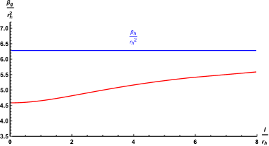
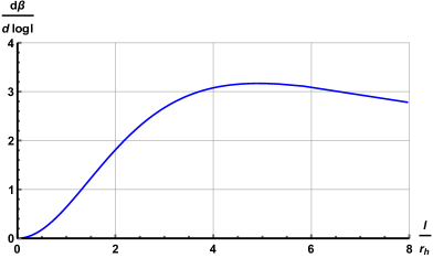
(a)	(b)

Figure 1: (a) Variation of $\frac{\beta_{g}}{r_{h}^{2}}=\frac{1}{T_{g}r_{h}^{2}}$ with subsystem length, (b) Renormalization Group flow (The $\frac{d\beta}{d\log l}$ axis has been scaled five times for visualization purpose)

4 Holographic subregion complexity

The subregion HC is proportional to the volume under the minimal hypersurface whose boundary coincides with the the boundary of the subsystem lying at the boundary at a fixed time. Using the approximation (17) in the expression for volume (16), we get

$$V=\frac{L}{r_{t}}\sum_{n=0}^{\infty}\sum_{m=0}^{\infty}\left(V_{1}+V_{2}+V_{3}\right)\left(\frac{r_{t}}{r_{h}}\right)^{2n+2m}$$ (53)

where

$$V_{1} = \frac{2\Gamma(n+\frac{1}{2})\Gamma(m+\frac{1}{2})}{\pi\;(2n+3)(2m+2n+1)\Gamma(n+1)\Gamma(m+1)}\delta^{2m+2n+1}$$

$$V_{2} = -\frac{\Gamma(n+\frac{1}{2})\Gamma(m+\frac{1}{2})}{4\sqrt{\pi}(m-1)\Gamma(n+1)\Gamma(m+1)\Gamma\left(\frac{2n+5}{4}\right)}\delta^{2m-2}$$

$$V_{3} = \frac{\Gamma(n+\frac{1}{2})\Gamma(m+\frac{1}{2})\Gamma\left(\frac{2m+2n+1}{4}\right)}{4\sqrt{\pi}(m-1)\Gamma(n+1)\Gamma(m+1)\Gamma\left(\frac{2m+2n+3}{4}\right)}\leavevmode\nobreak\ .$$ (54)

Now we should checkout for the divergences in the above mentioned terms as the expression for volume contains double sum which extends from $m,n=0$ to $\infty$. Due to the presence of the term $\left(\frac{r_{t}}{r_{h}}\right)^{2n+2m}$, we expect the divergence to occur near $r_{h}\rightarrow r_{t}$. We start analyzing the $V_{1}$ term. For large values of $(m,n)$, $V_{1}$ varies as

$$V_{1}\sim\frac{1}{n^{\frac{3}{2}}m^{\frac{1}{2}}(n+m)}<\frac{1}{n^{\frac{3}{2}}m^{\frac{3}{2}}}\leavevmode\nobreak\ .$$ (55)

We can now argue that $\sum_{n,m=0}^{\infty}V_{1}\left(\frac{r_{t}}{r_{h}}\right)^{2n+2m}$ is convergent. If $p(m,n)$ and $q(m,n)$ are two sequences of real numbers with $m$ and $n$ being positive integers, then the series $\sum_{n,m=0}^{\infty}p(m,n)$ is convergent if for each values of $(m,n)$ we have $|p(m,n)|\leq|q(m,n)|$. If we choose $q(m,n)=\frac{1}{n^{\frac{3}{2}}m^{\frac{3}{2}}}$, then $\sum_{n,m=0}^{\infty}\frac{1}{n^{\frac{3}{2}}m^{\frac{3}{2}}}=1/(\xi(3/2))^{2}$, where $\xi(3/2)$ is the Reimann Zeta function. Therefore the double sum over $V_{1}$ term converges absolutely. Moreover it is multiplied by $\delta^{2m+2n+1}$, which tends to zero. So we can neglect the contribution from $V_{1}$. Let us now look at the $V_{2}$ term which has a UV cutoff dependent term $\delta^{2m-2}$. For $m\geq 2$, this term will have negligible contribution but for $m=0,1$, this term is UV divergent. To get the exact form of UV divergence we compute the volume for $m=0$ and $1$ separately. It is expected that the $m=1$ term should give a logarithmic UV divergence. The volume integral for $m=0$ and $m=1$ are given by

$$V_{m=0} = \frac{L}{r_{t}}\sum_{n=0}^{\infty}\left(\frac{r_{t}}{r_{h}}\right)^{2n}\left(\frac{\Gamma(n+\frac{1}{2})\Gamma(\frac{3}{4}+\frac{n}{2})}{4\Gamma(n+1)\Gamma(\frac{5}{4}+\frac{n}{2})}\frac{1}{\delta^{2}}-\frac{\Gamma(n+\frac{1}{2})}{\sqrt{\pi}(2n+3)\Gamma(n+1)}\delta^{2n+1}\right.$$

$$\hskip 142.26378pt-\left.\frac{\Gamma(n+\frac{1}{2})\Gamma(\frac{1}{4}+\frac{n}{2})}{4\Gamma(n+1)\Gamma(\frac{3}{4}+\frac{n}{2})}\right)$$

$$V_{m=1} = \frac{L}{r_{t}}\sum_{n=0}^{\infty}\left(\frac{r_{t}}{r_{h}}\right)^{2n}\left(-\frac{\Gamma(n+\frac{1}{2})\Gamma(\frac{3}{4}+\frac{n}{2})}{4\Gamma(n+1)\Gamma(\frac{5}{4}+\frac{n}{2})}\log\delta+\frac{\Gamma(n+\frac{1}{2})}{\sqrt{\pi}(2n+3)\Gamma(n+1)}\delta^{2n+3}\log\delta\right.$$ (56)

$$\hskip 85.35826pt\left.+\frac{\Gamma(n+\frac{1}{2})\Gamma(\frac{3}{4}+\frac{n}{2})}{16\Gamma(n+1)\Gamma(\frac{5}{4}+\frac{n}{2})}\left(H_{n}\left[\frac{n}{2}-\frac{1}{4}\right]-H_{n}\left[\frac{n}{2}+\frac{1}{4}\right]\right)\right)\leavevmode\nobreak\ .$$

In the $r_{h}\rightarrow r_{t}$ limit, we use the expression for subsystem length (18) to get

$$V_{m=0}\sim\frac{lL}{(r_{h})^{2}}\left(\frac{b_{1}}{\delta^{2}}+b_{4}\right);\leavevmode\nobreak\ \leavevmode\nobreak\ \leavevmode\nobreak\ V_{m=1}\sim\frac{lL}{(r_{h})^{2}}\left(b_{2}\;\log\delta+b_{5}\right)$$ (57)

where $b_{1},b_{2},b_{3}$ and $b_{4}$ are numerical constants. Finally we look at the $V_{3}$ term. The analysis for $V_{3}$ term is more complicated. The detailed analysis is given in Appendix (A). This term in $r_{h}\rightarrow r_{t}$ limit varies as

$$V_{3}\sim\frac{l}{r_{h}}\left(b_{3}\frac{r_{h}}{l}+b_{6}\right)\leavevmode\nobreak\ .$$ (58)

Combining all these terms we get the volume to be

$$V\sim\frac{lL}{(r_{h})^{2}}\left(\frac{b_{1}}{\delta^{2}}+b_{2}\;\log\delta+b_{3}\frac{r_{h}}{l}+b_{7}\right)$$ (59)

where $b_{7}$ is another numerical constant. Therefore in terms of the black hole temperature, the expression for the finite part of holographic subregion complexity varies as

$$C_{finite}\sim T_{h}\left(b_{7}+b_{3}\frac{1}{\sqrt{T_{h}}}\right).$$ (60)

Therefore, the holographic entanglement entropy (33) and holographic subregion complexity (60) have the same kind of temperature dependence. We now proceed to evaluate the volume integral in the near horizon limit. In this limit the volume becomes

$$V=\frac{L}{r_{t}}\sum_{n=0}^{\infty}\sum_{m=0}^{\infty}\left(V_{1}+V_{2}+V_{3}\right)\left(\frac{r_{t}}{r_{h}}\right)^{n+m}$$ (61)

where

$$V_{1} = \frac{\Gamma(n+\frac{1}{2})\Gamma(m+\frac{1}{2})}{\pi\;(n+3)(m+n+1)\Gamma(n+1)\Gamma(m+1)}\delta^{m+n+1}$$

$$V_{2} = -\frac{\Gamma(n+\frac{1}{2})\Gamma(m+\frac{1}{2})}{4\sqrt{\pi}(m-2)\Gamma(n+1)\Gamma(m+1)\Gamma\left(\frac{n+5}{4}\right)}\delta^{m-2}$$

$$V_{3} = \frac{\Gamma(n+\frac{1}{2})\Gamma(m+\frac{1}{2})\Gamma\left(\frac{m+n+1}{4}\right)}{4\sqrt{\pi}(m-2)\Gamma(n+1)\Gamma(m+1)\Gamma\left(\frac{m+n+3}{4}\right)}\leavevmode\nobreak\ .$$ (62)

The terms $V_{1}$ and $V_{3}$ have almost the same pattern as in the previous case. So we can say that the term $V_{1}$ is convergent and have negligible contribution due to the UV cutoff $\delta^{m+n+1}$ and the term $V_{3}$ goes as

$$V_{3}\sim\frac{lL}{(r_{h})^{2}}\left(d_{5}\frac{r_{h}}{l}+d_{9}\right)\leavevmode\nobreak\ .$$ (63)

Now the term $V_{2}$ is divergent for $m\leq 2$, so we compute the volume term for $m=0,1,2$ separately (see Appendix (B)). In the limit $r_{h}\rightarrow r_{t}$, they behave as

$$V_{m=0}\sim\frac{lL}{(r_{h})^{2}}\left(d_{1}\frac{1}{\delta^{2}}+d_{6}\right)$$

$$V_{m=1}\sim\frac{lL}{(r_{h})^{2}}\left(d_{2}\frac{1}{\delta}+d_{7}\right)$$

$$V_{m=2}\sim\frac{lL}{(r_{h})^{2}}\left(d_{3}\log\delta+d_{8}\right)\leavevmode\nobreak\ .$$ (64)

Combining all the volume terms we get

$$V\sim\frac{lL}{(r_{h})^{2}}\left(d_{1}\frac{1}{\delta^{2}}+d_{2}\frac{1}{\delta}+d_{3}\log\delta+d_{10}+d_{5}\frac{r_{h}}{l}\right)\leavevmode\nobreak\ .$$ (65)

So the finite part of the holographic subregion complexity varies with the black hole temperature as

$$V_{finite}\sim T_{h}\left(d_{10}+b_{9}\frac{1}{\sqrt{T_{h}}}\right).$$ (66)

5 Fisher information metric and Fidelity susceptibility

In this section, we shall compute the Fisher information metric and the fidelity susceptibility for the Lifshitz black hole using holographic prescriptions [43, 44, 46]. In the context of quantum information theory there exists two well notions of distance between two quantum states. They are the Fisher information metric [47] and the fidelity susceptibility [48] (or called the Bures metric). From the literature [46], the definition of the Fisher information metric is given by

$$G_{F,\lambda\lambda}=\langle\delta\rho\;\delta\rho\rangle_{\lambda\lambda}^{(\sigma)}=\frac{1}{2}tr\left(\delta\rho\frac{d}{d(\delta\lambda)}\log(\sigma+\delta\lambda\delta\rho)|_{\delta\lambda=0}\right)$$ (67)

where $\delta\rho$ is a small deviation from the density matrix $\sigma$.

On the other hand the fidelity susceptibility is given by

$$G_{\lambda\lambda}=\partial^{2}_{\lambda}F;\leavevmode\nobreak\ \leavevmode\nobreak\ \leavevmode\nobreak\ \leavevmode\nobreak\ F=tr\sqrt{\sqrt{\sigma_{\lambda}}\rho_{\lambda+\delta\lambda}\sqrt{\sigma_{\lambda}}}$$ (68)

where $\rho$ and $\sigma$ are the final and initial density matrices, $F$ is called the fidelity between the two states.

The holographic computation of the Fisher information metric from relative EE was put forward in [43]. The Fisher information metric is given by

$${}G_{F,mm}=\frac{\partial^{2}}{\partial m^{2}}S_{rel}(\rho_{m}\parallel\rho_{0});\leavevmode\nobreak\ \leavevmode\nobreak\ \leavevmode\nobreak\ \leavevmode\nobreak\ \leavevmode\nobreak\ \leavevmode\nobreak\ \leavevmode\nobreak\ S_{rel}(\rho_{m}\parallel\rho_{0})=\Delta\langle H_{\rho_{0}}\rangle-\Delta S$$ (69)

where $m$ is a perturbation parameter, $\Delta S$ is the change in entanglement entropy from the vacuum state and $\Delta\langle H_{\rho_{0}}\rangle$ is the change in modular Hamiltonian. With this basic background in place we first compute the Fisher information metric for the Lifshitz black hole. We consider that the background is slightly perturbed from the pure Lifshitz spacetime but the subsystem length $l$ fixed. Then the inverse of the lapse function 8 can be written as

$$\frac{1}{f(r)}=\frac{1}{1-{r^{2}\over r_{h}^{2}}}=1+mr^{2}+m^{2}r^{4}.$$ (70)

where $m=\frac{1}{r_{h}^{2}}$, is the perturbation parameter in the bulk. As the underlying geometry has been changed from Lifshitz spacetime to asymptotic Lifshitz spacetime and we have not changed the subsystem length the turning point of the bulk extension will change as

$${}r_{t}=r_{t}^{(0)}+m\leavevmode\nobreak\ r_{t}^{(1)}+m^{2}\leavevmode\nobreak\ r_{t}^{(2)}$$ (71)

where $r_{t}^{(0)}$ is the turning point for pure Lifshitz spacetime and $r_{t}^{(1)}$, $r_{t}^{(2)}$ are first and second order corrections to the turning point.On the other hand the subsystem length $l$ can be obtained from (14,18) upto second order in perturbation as

$${}\frac{l}{r_{t}}=a_{0}+m\leavevmode\nobreak\ a_{1}r_{t}^{2}+m^{2}\leavevmode\nobreak\ a_{2}r_{t}^{4}$$ (72)

with

$$a_{0}=\frac{\sqrt{\pi}\Gamma\left(\frac{3}{4}\right)}{2\leavevmode\nobreak\ \Gamma\left(\frac{5}{4}\right)};\leavevmode\nobreak\ a_{1}=\frac{\Gamma\left(\frac{3}{2}\right)\Gamma\left(\frac{5}{4}\right)}{2\leavevmode\nobreak\ \Gamma\left(\frac{7}{4}\right)};\leavevmode\nobreak\ a_{2}=\frac{\Gamma\left(\frac{5}{2}\right)\Gamma\left(\frac{7}{4}\right)}{4\leavevmode\nobreak\ \Gamma\left(\frac{9}{4}\right)}.$$ (73)

Using the fact that the subsystem length is unchanged we obtain from equations (71,72), expressions for $r_{t}^{(0)}$, $r_{t}^{(1)}$ and $r_{t}^{(2)}$ as given below

$$\frac{l}{r_{t}^{(0)}}=a_{0},\leavevmode\nobreak\ \leavevmode\nobreak\ r_{t}^{(1)}=-\frac{a_{1}}{a_{0}}(r_{t}^{(0)})^{3},\leavevmode\nobreak\ \leavevmode\nobreak\ r_{t}^{(2)}=\left(3\frac{a_{1}^{2}}{a_{0}^{2}}-\frac{a_{2}}{a_{0}}\right)(r_{t}^{(0)})^{5}\leavevmode\nobreak\ \leavevmode\nobreak\ .$$ (74)

The expression for extremal area of the bulk extension upto second order in perturbation parameter can be obtained from eq.(15, 25) as

$$A=\frac{2L}{r_{c}}-a_{0}\frac{L}{r_{t}}+3a_{1}Lr_{t}m+\frac{5}{3}a_{2}Lr_{t}^{3}m^{2}.$$ (75)

As we are interested in computing the change in area due to a slight change in background we use (71) to recast the above expression for area in the following form

$$A=A^{(0)}+m\leavevmode\nobreak\ A^{(1)}+m^{2}\leavevmode\nobreak\ A^{(2)}$$ (76)

where $A^{(0)}$, $A^{(1)}$ and $A^{(2)}$ are area for pure Lifshitz spacetime, first order and second order corrections to the area for change in background. They have the following expressions

$$A^{(0)}=\frac{2L}{r_{c}}-a_{0}\frac{L}{r_{t}^{(0)}},\leavevmode\nobreak\ \leavevmode\nobreak\ A^{(1)}=2a_{1}Lr_{t}^{(0)},\leavevmode\nobreak\ \leavevmode\nobreak\ A^{(2)}=\left(\frac{2}{3}a_{2}-\frac{a_{1}^{2}}{a_{0}}\right)L(r_{t}^{(0)})^{3}.$$ (77)

It has been shown in [43] that at first order in $m$ the relative entropy vanishes and in second order in $m$ the relative entropy is given by $S_{rel}=-\Delta S$. Hence,

$$S_{rel}=-m^{2}\frac{A^{(2)}}{4G}=m^{2}\frac{Ll^{3}}{4G}\left(\frac{3a_{1}^{2}-2a_{0}a_{2}}{3a_{0}^{4}}\right).$$ (78)

From eq. (69), the Fisher information metric therefore reads

$$G_{F,mm}=\frac{Ll^{3}}{2G}\left(\frac{3a_{1}^{2}-2a_{0}a_{2}}{3a_{0}^{4}}\right).\leavevmode\nobreak\ .$$ (79)

In [46], a proposal for computing the above quantity was given. The proposal is to consider the difference of two volumes yielding a finite expression

$$\mathcal{F}=C_{d}(V-V_{(0)})$$ (80)

where $V$ is evaluated for a second order perturbation around pure Lifshitz spacetime . $C_{d}$ is a dimensionless constant which cannot be fixed from the first principles of the gravity side. We shall now apply this proposal to compute the Fisher information metric for the Lifshitz black hole. The change in volume under Ryu-Takayanagi minimal surface at second order in perturbation takes the form

$$V=V^{(0)}+mV^{(1)}+m^{2}V^{(2)}$$ (81)

with

$$V^{(0)}=\frac{Ll}{2r_{c}^{2}}-\frac{a_{0}^{2}L}{2l},\leavevmode\nobreak\ \leavevmode\nobreak\ V^{(1)}=-mLl\left(\frac{a_{1}}{2a_{0}}+\frac{6-\pi}{8}\right),\leavevmode\nobreak\ \leavevmode\nobreak\ V^{(2)}=m^{2}\frac{Ll^{3}}{a_{0}^{3}}\left(\frac{a_{1}^{2}}{a_{0}}-\frac{a_{2}}{2}+\frac{13-3\pi}{12}a_{1}\right).$$ (82)

The holographic dual of Fisher information metric is now defined as

$${}G_{F,mm}=\partial_{m}^{2}\mathcal{F};\leavevmode\nobreak\ \leavevmode\nobreak\ \leavevmode\nobreak\ \leavevmode\nobreak\ \leavevmode\nobreak\ \leavevmode\nobreak\ \mathcal{F}=C_{d}\left(V-V_{(0)}\right)$$ (83)

with the constant $C_{d}$ to be determined by requiring that the holographic dual Fisher information metric from the above equation must agree with that obtained from the relative entropy (79). The constant $C_{d}$ is therefore given by

$${}C_{d}=\frac{3a_{1}^{2}-2a_{0}a_{2}}{G(12a_{1}^{2}-6a_{0}a_{2}+(13-3\pi)a_{0}a_{1})}\leavevmode\nobreak\ .$$ (84)

We now look forward to compute the fidelity susceptibility holographically. If one assumes that the states depend on a single parameter $\lambda$ then for pure states the fidelity (68) reduces to

$$\langle\Psi(\lambda)|\Psi(\lambda+\delta\lambda)\rangle=1-G_{\lambda\lambda}(\delta\lambda)^{2}+\cdots\leavevmode\nobreak\ .$$ (85)

The above expression immediately suggests that $G_{\lambda\lambda}$ is a measure of distance between two quantum states called the fidelity susceptibility . The holographic prescription for evaluating the fidelity susceptibility in ($d+1$) - dimensional $AdS$ spacetime is given by [44]

$${}G_{\lambda\lambda}=n_{d-1}\frac{Vol(\Sigma_{max})}{R^{d}}$$ (86)

where $\Sigma_{max}$ is the maximum volume in the bulk that ends at the boundary of the bulk at a fixed time slice. $R$ is the radius of curvature of $AdS$ spacetime and $n_{d-1}$ is a $\mathcal{O}(1)$ constant.

For our case the fidelity susceptibility reads

$$G_{\lambda\lambda} = n_{2}Ll\int_{r_{c}}^{r_{h}}dr\frac{1}{r^{3}\sqrt{1-{r^{2}\over r_{h}^{2}}}}$$ (87)

$$= \frac{n_{2}Ll}{r_{h}^{2}}\left(\frac{r_{h}^{2}}{2r_{c}^{2}}+B(-1,\frac{1}{2})\right).$$

We see that the above expression for the fidelity susceptibility does not agree with the Fisher information metric obtained in eq.(79).

6 Conclusion

In this paper, we have computed different information theoretic quantities holographically in the context of a non-relativistic ($3+1$)-dimensional Lifshitz black hole. Our main focus has been the following. To begin with we have looked at the Ryu-Takayanagi area which is related to the holographic entanglement entropy and second is the minimal volume under the Ryu-takayanagi area which is related to holographic subregion complexity. The finite part of the holographic entanglement entropy approaches the black hole entropy in the infrared ($r_{t}\rightarrow r_{h}$) regime. This clearly depicts that the entanglement entropy becomes thermal entropy in the high temperature limit even in the non-relativistic background. In the ultra-violet ($r_{t}\ll r_{h}$) limit, the finite part of holographic entanglement entropy goes as $S_{finite}^{(UV)}\sim\frac{1}{l}\left(constant+\mathcal{O}(l^{2})\right)$. This result departs with respect to the subleading terms from the relativistic counterpart comprising the $(3+1)$-dimensional $SAdS$ black hole where $S_{finite}^{(UV)}\sim\frac{1}{l}\left(constant+\mathcal{O}(l^{3})\right)$. Further, the holographic entanglement entropy has a logarithmic divergence in addition to the usual $1/\delta$ divergence in the near horizon approximation. We have then introduced the notion of a generalized temperature in terms of the renormalized holographic entanglement entropy. The variation of the generalized temperature with the subsystem length $l$ shows that the generalized temperature reduces to the black hole temperature, that is the Hawking temperature, at large subsystem length (infrared limit). This therefore implies that our choice of the definition for the generalized temperature is correct. It has been observed that the generalized temperature leads to a thermodynamics like law $E=T_{g}S_{REE}$. It is also interesting to note that the generalized temperature has a constant value in the ultraviolet limit ($l\rightarrow 0$). This is a new result which does not have any counterpart in the relativistic background, namely, the $(3+1)$-dimensional $SAdS$ black hole. We have then observed departures from relativistic results in case of the holographic subregion complexity. Both in the $3+1$-dimensional relativistic and non-relativistic cases, the holographic subregion complexity suffers $1/\delta^{2}$ divergences, but in the non-relativistic case we have $\log\delta$ divergence which was absent in the relativistic case. The near horizon approximation have the same type of divergences in both the cases. The holographic Fisher information metric has been computed next from the concept of relative entropy [43]. We have also computed the holographic subregion complexity in the ulta-violet limit upto second order in the perturbation parameter. Using the proposal in [46], we have used this result to obtain an expression for the Fisher information metric upto an undetermined constant. We have equated this result of the Fisher information metric with that obtained from the relative entropy to determine the undetermined constant. The constant is found to be a number. The holographic fidelity susceptibility has also been computed. We find that there is a mismatch between the expressions for the Fisher information metric and the holographic fidelity susceptibility. These two quantities are related in the context of quantum information. A possible reason for this mismatch may be the following. In case of the Fisher information metric, an integration up to the turning point of the Ryu-takayanagi surface is performed. However, in case of the fidelity susceptibility, an integration up to the horizon radius of the black is involved. A similar observation has already been made in the relativistic background in [38].

Appendix

Appendix A Analysis of $V_{3}$ term of volume

The $V_{3}$ term as given in equation (4) for large $(m,n)$ goes as

$$V_{3}\sim\frac{1}{m^{3/2}\sqrt{n(m+n)}}.$$ (88)

So the sum over $n$ is divergent by comparison test. We perform the sum over $m$ to get

$$V_{3} = \sum_{n=0}^{\infty}\sum_{m=0}^{\infty}\left(\frac{r_{t}}{r_{h}}\right)^{2n+2m}\frac{\Gamma(n+\frac{1}{2})\Gamma(m+\frac{1}{2})\Gamma\left(\frac{2m+2n+1}{4}\right)}{4\sqrt{\pi}(m-1)\Gamma(n+1)\Gamma(m+1)\Gamma\left(\frac{2m+2n+3}{4}\right)}$$ (89)

$$= \sum_{n=0}^{\infty}\left(\frac{r_{t}}{r_{h}}\right)^{2n}\frac{\Gamma(n+\frac{1}{2})}{128\;\Gamma(n+1)}\left(\frac{5\Gamma(\frac{2n+7}{4})}{\Gamma(\frac{2n+9}{4})}\;HPFQR\left[\{1,1,\frac{7}{4},\frac{9}{4},\frac{9}{4}+\frac{n}{2}\},\{2,2,\frac{5}{2},\frac{9}{4}+\frac{n}{2}\},1\right]\right.$$

$$\left.\hskip 85.35826pt-\frac{32\Gamma(\frac{2n+1}{4})}{\Gamma(\frac{2n+3}{4})}\;HPFQR\left[\{-\frac{1}{2},\frac{1}{2},\frac{3}{4},\frac{1}{4}+\frac{n}{2}\},\{\frac{1}{2},\frac{1}{2},\frac{3}{4}+\frac{n}{2}\},1\right]\right)$$

where $HPFQR$ is the $HypergeometricPFQRegularized$ function. For large values of $n$ the summation term varies as $\sim\frac{1}{n}\left(\frac{r_{t}}{r_{h}}\right)^{2n}$. On the other hand the expression for length $\left(\frac{l}{r_{t}}\right)$ as presented in (18) also varies as $\sim\frac{1}{n}\left(\frac{r_{t}}{r_{h}}\right)^{2n}$ in large $n$ limit. Therefore in $r_{h}\rightarrow r_{t}$ limit the $V_{3}$ term varies as

$$V_{3}\sim\left(a\frac{l}{r_{h}}+b\right)$$ (90)

where $a,b$ are numerical constants.

Appendix B Exact computation of Volume for $m=0,1,2$ in near horizon limit

$$V_{m=0} = \frac{L}{r_{t}}\sum_{n=0}^{\infty}\left(\frac{r_{t}}{r_{h}}\right)^{n}\frac{\Gamma(n+\frac{1}{2})}{\sqrt{\pi}\Gamma(n+1)}\left(\int_{0}^{1}du\;\frac{u^{n+2}}{\sqrt{1-u^{4}}}\int_{\delta}^{1}du\;\frac{1}{u^{3}}-\int_{\delta}^{1}du\;\frac{1}{u^{3}}\int_{0}^{u}ds\frac{s^{n+2}}{\sqrt{1-u^{4}}}\right)$$ (91)

$$= \frac{L}{r_{t}}\left(\sum_{n=0}^{\infty}\left(\frac{r_{t}}{r_{h}}\right)^{n}\frac{\Gamma(n+\frac{1}{2})\Gamma(\frac{n+3}{4})}{8\;\Gamma(n+1)\Gamma(\frac{n+5}{4})}\frac{1}{\delta^{2}}-\sum_{n=0}^{\infty}\left(\frac{r_{t}}{r_{h}}\right)^{n}\frac{\Gamma(n+\frac{1}{2})\Gamma(\frac{n+1}{4})}{8\;\Gamma(n+1)\Gamma(\frac{n+3}{4})}\right)$$

$$= \frac{L}{r_{t}}\left(\frac{l}{2\sqrt{2}\;r_{t}}\frac{1}{\delta^{2}}-\sum_{n=0}^{\infty}\left(\frac{r_{t}}{r_{h}}\right)^{n}\frac{\Gamma(n+\frac{1}{2})\Gamma(\frac{n+1}{4})}{8\;\Gamma(n+1)\Gamma(\frac{n+3}{4})}\right),$$

where in the last line we have used the expression for subsystem length in near horizon limit (36).

$$V_{m=1} = \frac{L}{r_{t}}\sum_{n=0}^{\infty}\left(\frac{r_{t}}{r_{h}}\right)^{n+1}\frac{\Gamma(n+\frac{1}{2})}{2\sqrt{\pi}\Gamma(n+1)}\left(\int_{0}^{1}du\;\frac{u^{n+2}}{\sqrt{1-u^{4}}}\int_{\delta}^{1}du\;\frac{1}{u^{2}}-\int_{\delta}^{1}du\;\frac{1}{u^{2}}\int_{0}^{u}ds\frac{s^{n+2}}{\sqrt{1-u^{4}}}\right)$$ (92)

$$= \frac{L}{r_{t}}\left(\sum_{n=0}^{\infty}\left(\frac{r_{t}}{r_{h}}\right)^{n+1}\frac{\Gamma(n+\frac{1}{2})\Gamma(\frac{n+3}{4})}{8\;\Gamma(n+1)\Gamma(\frac{n+5}{4})}\frac{1}{\delta}-\sum_{n=0}^{\infty}\left(\frac{r_{t}}{r_{h}}\right)^{n}\frac{\Gamma(n+\frac{1}{2})\Gamma(\frac{n+2}{4})}{8\;\Gamma(n+1)\Gamma(\frac{n+4}{4})}\right)$$

$$= \frac{L}{r_{t}}\left(\frac{l}{2\sqrt{2}\;r_{t}}\frac{1}{\delta}-\sum_{n=0}^{\infty}\left(\frac{r_{t}}{r_{h}}\right)^{n}\frac{\Gamma(n+\frac{1}{2})\Gamma(\frac{n+2}{4})}{8\;\Gamma(n+1)\Gamma(\frac{n+4}{4})}\right)$$

and

$$V_{m=2} = \frac{L}{r_{t}}\sum_{n=0}^{\infty}\left(\frac{r_{t}}{r_{h}}\right)^{n+2}\frac{3\;\Gamma(n+\frac{1}{2})}{8\sqrt{\pi}\Gamma(n+1)}\left(\int_{0}^{1}du\;\frac{u^{n+2}}{\sqrt{1-u^{4}}}\int_{\delta}^{1}du\;\frac{1}{u}-\int_{\delta}^{1}du\;\frac{1}{u}\int_{0}^{u}ds\frac{s^{n+2}}{\sqrt{1-u^{4}}}\right)$$ (93)

$$= \frac{L}{r_{t}}\sum_{n=0}^{\infty}\left(\frac{r_{t}}{r_{h}}\right)^{n+2}\frac{3\;\Gamma(n+\frac{1}{2})}{8\sqrt{\pi}\Gamma(n+1)}\left(-\frac{\sqrt{\pi}\Gamma(\frac{n+3}{4})}{4\Gamma(\frac{n+5}{4})}\log\delta+\frac{\delta^{n+3}\log\delta}{n+3}\right.$$

$$\left.\hskip 142.26378pt+\frac{\sqrt{\pi}\Gamma(\frac{n+3}{4})}{16\Gamma(\frac{n+5}{4})}\left(H_{n}(\frac{n-1}{4})-H_{n}(\frac{n+1}{4})\right)\right)$$

$$\approx \frac{L}{r_{t}}\left(-\frac{3\sqrt{2\;}l}{16\;r_{t}}\log\delta+\sum_{n=0}^{\infty}\left(\frac{r_{t}}{r_{h}}\right)^{n+2}\frac{3\;\Gamma(n+\frac{1}{2})\Gamma(\frac{n+3}{4})}{128\Gamma(n+1)\Gamma(\frac{n+5}{4})}\left(H_{n}(\frac{n-1}{4})-H_{n}(\frac{n+1}{4})\right)\right)$$

References

- [1] E. Witten, Adv. Theor. Math. Phys. 2 (1998) 253
- [2] J. M. Maldacena, Int. J. Theor. Phys. 38 (1999) 1113 [Adv. Theor. Math. Phys. 2 (1998) 231]
- [3] O. Aharony, S. S. Gubser, J. M. Maldacena, H. Ooguri and Y. Oz, Phys. Rept. 323 (2000) 183
- [4] P. Calabrese, J. L. Cardy, “Entanglement entropy and quantum field theory”, J. Stat. Mech. 0406 (2004) P06002.
- [5] P. Calabrese, J. L. Cardy, “Entanglement entropy and quantum field theory: A Non-technical introduction”, Int. J. Quant. Inf. 4 (2006) 429.
- [6] G. Vidal, J. I. Latorre, E. Rico and A. Kitaev, “Entanglement in quantum critical phenomena,” Phys. Rev. Lett. 90 (2003) 227902
- [7] A. Kitaev and J. Preskill, “Topological entanglement entropy,” Phys. Rev. Lett. 96 (2006) 110404
- [8] M. Levin and X. G. Wen, “Detecting topological order in a ground state wave function”, Phys. Rev. Lett. 96 (2006) 110405
- [9] S. A. Hartnoll, “Lectures on holographic methods for condensed matter physics,” Class. Quant. Grav. 26 (2009) 224002
- [10] R. G. Cai, S. He, L. Li and Y. L. Zhang, “Holographic Entanglement Entropy in Insulator/Superconductor Transition,” JHEP 1207 (2012) 088
- [11] J. Casalderrey-Solana, H. Liu, D. Mateos, K. Rajagopal and U. A. Wiedemann, “Gauge/String Duality, Hot QCD and Heavy Ion Collisions,” book:Gauge/String Duality, Hot QCD and Heavy Ion Collisions. Cambridge, UK: Cambridge University Press, 2014 [arXiv:1101.0618 [hep-th]].
- [12] S. Ryu, T. Takayanagi, “Holographic derivation of entanglement entropy from AdS/CFT”, Phys. Rev. Lett. 96 (2006) 181602.
- [13] S. Ryu, T. Takayanagi, “Aspects of Holographic Entanglement Entropy”, JHEP 0608 (2006) 045.
- [14] J. Bhattacharya, M. Nozaki, T. Takayanagi, T. Ugajin, Phys. Rev. Lett. 110 (2013) 091602.
- [15] D. Allahbakhshi, M. Alishahiha, A. Naseh, JHEP 1308 (2013) 102.
- [16] S. N. Solodukhin, Phys. Rev. Lett. 97 (2006) 201601
- [17] V. E. Hubeny, JHEP 1207 (2012) 093 doi:10.1007/JHEP07(2012)093
- [18] P. Chaturvedi, V. Malvimat and G. Sengupta, Phys. Rev. D 94 (2016) no.6, 066004
- [19] S. Karar, D. Ghorai and S. Gangopadhyay, Nucl. Phys. B 938 (2019) 363
- [20] A. Saha, S. Karar and S. Gangopadhyay, Eur. Phys. J. Plus 135 (2020) no.2, 132
- [21] K. S. Kim and C. Park, Phys. Rev. D 95 (2017) no.10, 106007 doi:10.1103/PhysRevD.95.106007
- [22] A. Saha, S. Gangopadhyay and J. P. Saha, Phys. Rev. D 100 (2019) no.10, 106008 doi:10.1103/PhysRevD.100.106008
- [23] M. Alishahiha, Phys. Rev. D 92 (2015) 126009.
- [24] L. Susskind, Fortsch.Phys. 64 (2016) 24, Addendum: Fortsch.Phys. 64 (2016) 44-48.
- [25] D. Stanford, L. Susskind, Phys. Rev. D 90 (2014) 126007.
- [26] A.R. Brown, D.A. Roberts, L. Susskind, B. Swingle, Y. Zhao, Phys. Rev. D 93 (2016) no.8, 086006.
- [27] O. Ben-Ami and D. Carmi, JHEP 1611 (2016) 129
- [28] J. Couch, W. Fischler, P. H. Nguyen, JHEP 1703 (2017) 119.
- [29] S. Chapman, H. Marrochio and R. C. Myers, JHEP 1701 (2017) 062.
- [30] D. Carmi, R. C. Myers, P. Rath, JHEP 1703 (2017) 118.
- [31] D. Carmi, S. Chapman, H. Marrochio, R. C. Myers and S. Sugishita, JHEP 1711 (2017) 188.
- [32] P. Caputa, N. Kundu, M. Miyaji, T. Takayanagi and K. Watanabe, JHEP 1711 (2017) 097.
- [33] C. A. Agón, M. Headrick, B. Swingle, JHEP 1902 (2019) 145.
- [34] S. Chapman, H. Marrochio and R. C. Myers, JHEP 1806 (2018) 046.
- [35] S. Chapman, H. Marrochio, R.C. Myers, JHEP 1806 (2018) 114.
- [36] S. Karar, S. Gangopadhyay and A. S. Majumdar, Int. J. Mod. Phys. A 34 (2019) no.01, 1950003
- [37] A. Ghosh and R. Mishra, arXiv:1907.11757 [hep-th].
- [38] S. Karar, R. Mishra and S. Gangopadhyay, Phys. Rev. D 100 (2019) no.2, 026006 doi:10.1103/PhysRevD.100.026006
- [39] S. Chakraborty, P. Dey, S. Karar, S. Roy, JHEP 1504 (2015) 133.
- [40] S. Karar, S. Gangopadhyay, Phys. Rev. D 98 (2018) no.2, 026029.
- [41] K. Balasubramanian and J. McGreevy, Phys. Rev. D 80 (2009) 104039 doi:10.1103/PhysRevD.80.104039
- [42] P. Roy and T. Sarkar, Phys. Rev. D 96 (2017) no.2, 026022 doi:10.1103/PhysRevD.96.026022
- [43] N. Lashkari and M. Van Raamsdonk, JHEP 1604 (2016) 153 doi:10.1007/JHEP04(2016)153
- [44] M. Miyaji, T. Numasawa, N. Shiba, T. Takayanagi, K. Watanabe, Phys. Rev. Lett. 115 (2015) no.26, 261602 doi:10.1103/PhysRevLett.115.261602.
- [45] S. Kachru, X. Liu and M. Mulligan, Phys. Rev. D 78 (2008) 106005 doi:10.1103/PhysRevD.78.106005
- [46] S. Banerjee, J. Erdmenger, D. Sarkar, JHEP 1808 (2018) 001.
- [47] M. G. Paris, “Quantum estimation for quantum technology,” International Journal of Quantum Information 07 (2009) 125.
- [48] Bures, D, “An Extension of Kakutani’s Theorem on Infinite Product Measures to the Tensor Product of Semifinite w*-Algebras,” Transactions of the American Mathematical Society,135 (1969) 199-212. doi:10.2307/1995012