Weakly Supervised Semantic Segmentation of Satellite Images for Land Cover Mapping – Challenges and Opportunities

Abstract

Fully automatic large-scale land cover mapping belongs to the core challenges addressed by the remote sensing community. Usually, the basis of this task is formed by (supervised) machine learning models. However, in spite of recent growth in the availability of satellite observations, accurate training data remains comparably scarce. On the other hand, numerous global land cover products exist and can be accessed often free-of-charge. Unfortunately, these maps are typically of a much lower resolution than modern day satellite imagery. Besides, they always come with a significant amount of noise, as they cannot be considered ground truth, but are products of previous (semi-)automatic prediction tasks. Therefore, this paper seeks to make a case for the application of weakly supervised learning strategies to get the most out of available data sources and achieve progress in high-resolution large-scale land cover mapping. Challenges and opportunities are discussed based on the SEN12MS dataset, for which also some baseline results are shown. These baselines indicate that there is still a lot of potential for dedicated approaches designed to deal with remote sensing-specific forms of weak supervision.

1 Introduction

The problem of automatic land cover mapping from remote sensing imagery is traditionally cast as a (supervised) machine learning task, especially when applied to large study areas [Cihlar, 2000]. However, while the amount of available satellite data keeps on growing, training labels remain rare, because of the difficulty to create reliable land cover annotations that can be referred to as “ground truth”. On the other hand, manifold large-scale land cover datasets already exist, all of which are the result of (semi-)automated processes themselves. This introduces weakly supervised learning as a promising strategy to train well-generalizing models on available data – even if the labels come with a significant error bar or at comparably low resolutions.

In this paper, we discuss the problem of weakly supervised learning of models for land cover prediction from satellite data. For this purpose, we focus on the freely available global imagery provided by the Sentinel-1 and Sentinel-2 missions of the European Copernicus program [Torres et al., 2012, Drusch et al., 2012] and a simplified version of the land cover classification scheme of the International Geosphere-Biosphere Programme (IGBP) [Loveland, Belward, 1997], which is reflected by the SEN12MS dataset [Schmitt et al., 2019] and the 2020 IEEE-GRSS Data Fusion Contest (DFC2020) [Yokoya et al., 2020]. Besides a description of the challenge and how SEN12MS and DFC2020 are addressing it, baseline results using off-the-shelf deep learning models are provided to highlight the importance of dedicated research.

2 Weakly Supervised Learning

In his excellent review, [Zhou, 2018] defines weakly supervised learning as an umbrella term addressing the attempt to construct predictive models from three types of weak supervision:

• Incomplete supervision
  In this case, a small amount of labeled data, which is insufficient to train a good model and abundant unlabeled data are available.

• Inexact supervision
  In this case, some supervision information is given, but it is not as exact as necessary. An example of this is land cover labels, which have a lower resolution than the satellite observations that shall be processed.

• Inaccurate supervision
  In this case, annotations cannot be considered as ground-truth; i.e., at least some of the labels are erroneous.

In the context of this paper, weakly supervised learning is restricted to the cases of inexact and inaccurate supervision, which can also be seen as different forms of label noise. In contrast to that, incomplete supervision is seen as a different case, which is addressed by semi-supervised learning [Zhu, Goldberg, 2009], which is not covered here. As shown in the following sections, dealing with different forms of noisy samples has become a well-addressed field in machine learning and should receive quite some attention by remote sensing researchers as well.

2.1 Machine Learning with Noisy Samples

Weakly supervised learning in the above-defined sense, i.e. learning from inexact and inaccurate samples, has become a sub-field in machine learning research that has been drawing a significant amount of interest. While there are some studies, which indicate that deep neural networks are relatively robust to label noise [Rolnick et al., 2018], many researchers investigate approaches to deal with this challenge based on insights from robust statistics and dedicated mathematical modelling. Thus, popular solutions in this context are either the formulation of robust loss functions, e.g. [Ghosh et al., 2017], the iterative improvement of training data via bootstrapping [Reed et al., 2015], or the addition of dedicated noise layers to the neural network [Sukhbaatar et al., 2015]. As summarized in [Frenay, Verleysen, 2014], it can be stated that numerous possible coping strategies exist.

2.2 Relevance for the Remote Sensing of Land Cover

Remote sensing has long been a primary source of big data [Chi et al., 2016], with the numbers of available observations and measurements of our planet continuously on the rise. Driven by this development, deep learning has drawn significant attention from the research community [Zhu et al., 2017]. However, as highlighted by [Reichstein et al., 2019], the lack of dedicated large training or benchmark datasets still remains one of the grand challenges in the creation of operational models for real-world applications. On the other hand, past efforts of remote sensing scientists and practitioners have led to the production of numerous large-scale – or even global – land cover maps. As nicely summarized by [Grekousis et al., 2015], the resolutions of those maps typically range from $30$m to $1{,}000$m per pixel with overall accuracies between $64\%$ and $88\%$. In other words, plenty of noisy training labels are potentially available free of charge! Inspired by the generic techniques for machine learning from noisy samples described in the previous section, one would think that weakly supervised learning of land cover prediction models using these available datasets as training input would have become a major theme in modern day remote sensing research. Interestingly, however, the literature dedicated to this challenge is still rather scarce. While most papers addressing weak supervision in a remote sensing context deal with object detection, e.g. [Zhang et al., 2015, Kellenberger et al., 2019], the few papers addressing weakly supervised semantic segmentation usually rely on sparse or even only image-level annotations, e.g. [Fu et al., 2018, Wang et al., 2020], instead of coarse and/or noisy labels available in a dense manner. A quite notable exception is the work by [Robinson et al., 2019], who fused low-resolution and high-resolution labels in order to produce a high-resolution land cover map of the contiguous United States. Their approach is based on what they called super-resolution loss in an earlier contribution [Malkin et al., 2019], which allows to predict high-resolution land cover from low-resolution labels by modeling the expected distribution of high-resolution land cover and using its distance to the predicted distribution as an additional loss term.

Using the SEN12MS dataset, which combines noisy land cover labels with a resolution of $500$m with Sentinel-1 SAR and Sentinel-2 optical data, as an example, this paper seeks to provide a basis for further explorations of weakly supervised semantic segmentation of satellite images for land cover prediction.

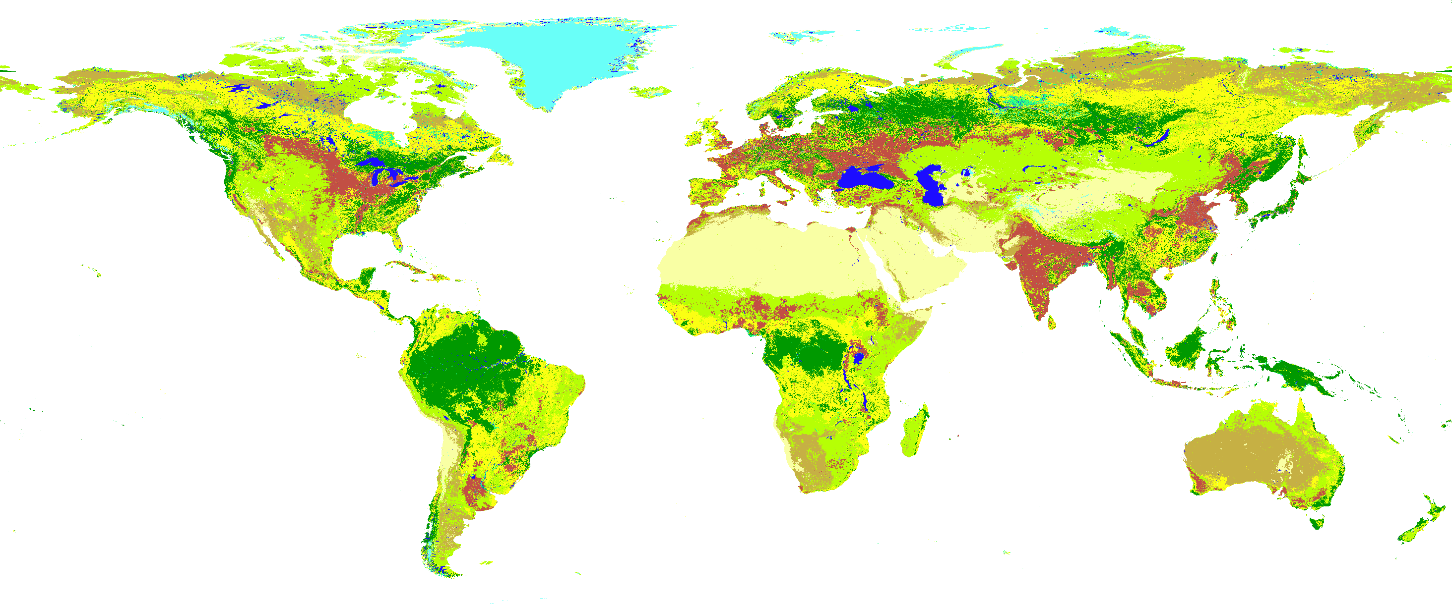
Figure 1: The MODIS-derived world map at a resolution of $500$m following the simplified IGBP scheme. While larger areas of the Savanna class (in yellow color) are found in South America, Africa and Australia as expected, there are also vast areas of Savanna in Canada, Scandinavia, and Siberia – regions in which savannas in the geographical sense of the term usually do not exist.

3 Weakly Supervised Learning for Land Cover Mapping with SEN12MS

IGBP Class Number	IGBP Class Name	Simplified Class Number	Simplified Class Name	Color
1	Evergreen Needleleaf Forest	1	Forest	009900
2	Evergreen Broadleaf Forest
3	Deciduous Needleleaf Forest
4	Deciduous Broadleaf Forest
5	Mixed Forest
6	Closed Shrublands	2	Shrubland	c6b044
7	Open Shrublands
8	Woody Savannas	3	Savanna	fbff13
9	Savanna
10	Grasslands	4	Grassland	b6ff05
11	Permanent Wetlands	5	Wetlands	27ff87
12	Croplands	6	Croplands	c24f44
14	Cropland / Natural Vegetation Mosaics
13	Urban and Built-up Lands	7	Urban/Built-up	a5a5a5
15	Permanent Snow and Ice	8	Snow/Ice	69fff8
16	Barren	9	Barren	f9ffa4
17	Water Bodies	10	Water	1c0dff

Table 1: The simplified IGBP land cover classification scheme.

The SEN12MS dataset [Schmitt et al., 2019] was published in 2019 as the largest curated dataset dedicated to deep learning in remote sensing at that time. It consists of $180{,}662$ patch triplets sampled over all meteorological seasons and all inhabited continents in order to represent a global distribution. Every triplet consists of a dual-polarimetric Sentinel-1 SAR image, a multi-spectral Sentinel-2 image tensor, and four different land cover maps following different internationally established classification schemes. In the frame of the 2020 IEEE-GRSS Data Fusion Contest (DFC2020), the organizers defined the weakly supervised training of globally applicable land cover prediction models as the contest goal [Yokoya et al., 2020].

3.1 The Simplified IGBP Land Cover Classification Scheme

For the DFC2020 the IGBP classification scheme, which originally is comprised of 17 classes [Loveland, Belward, 1997], was aggregated to 10 less fine-grained classes (see Tab. 1). This simplified IGBP scheme is similar to the classification scheme adopted by the authors of the FROM-GLC10 dataset [Gong et al., 2019], which constitutes the first global land cover map with a resolution of $10$m (at an overall validation accuracy of about $73\%$). Both schemes differ in only one class: While the simplified IGBP scheme contains a Savanna class, the FROM-GLC10 scheme contains a Tundra class. However, both classes are restricted to certain geographical regions: According to the Encyclopedia Britannica, a savanna “is characterized by an open tree canopy (i.e., scattered trees) above a continuous tall grass understory (the vegetation layer between the forest canopy and the ground)”. Mostly found “in Africa, South America, Australia, India, the Myanmar (Burma)-Thailand region in Asia, and Madagascar”, savannas thus are a land cover type, which can not be found around the globe, but only in specific geographical regions. Above that, they are also not suitable for classical pixel-based classification approaches, since at a resolution of $10$m no Savanna pixels exist – one will either find pixels containing trees (i.e. the Forest class in simplified IGBP terms), or grass (i.e. Grassland). At a resolution of $500$m, however, the mixing of the spectral responses of sparse trees and grass understory can well lead to a distinct spectral Savanna profile. It has to be noted that this is different for approaches that take spatial context into account as do, for example, convolutional neural networks – as long as their receptive field is large enough.

As can be seen in Fig. 1, in the MODIS-derived IGBP land cover map, which constitutes the basis of the SEN12MS land cover annotations, the Savanna class is way more widely spread than one would expect based on the above-mentioned definition, even outside those regions where savannas actually exist, which should be considered as a form of systematic label noise. For generic solutions to global land cover mapping, it will thus be advisable to adapt suitable strategies that either ignore training pixels with Savanna label, or that allow a transformation of Savanna into classes such as Grassland, or Forest, which are applicable in all regions of the world. Since there is certainly no one-to-one mapping between Savanna and the alternative classes, statistical strategies such as, e.g., the one proposed by [Malkin et al., 2019] are in need.

3.2 SEN12MS

The distribution of the pixels contained in the SEN12MS dataset over the 10 classes of the simplified IGBP scheme is shown in Fig. 2. While the distribution is relatively balanced in terms of the classes Forest, Grassland, Croplands, and Urban, the classes Shrubland, Barren, and Water are slightly less frequent. The major outliers are the classes Wetlands and Snow/Ice, which hardly exist, and the largest class Savanna, which accounts for almost a quarter of all pixels in the dataset.

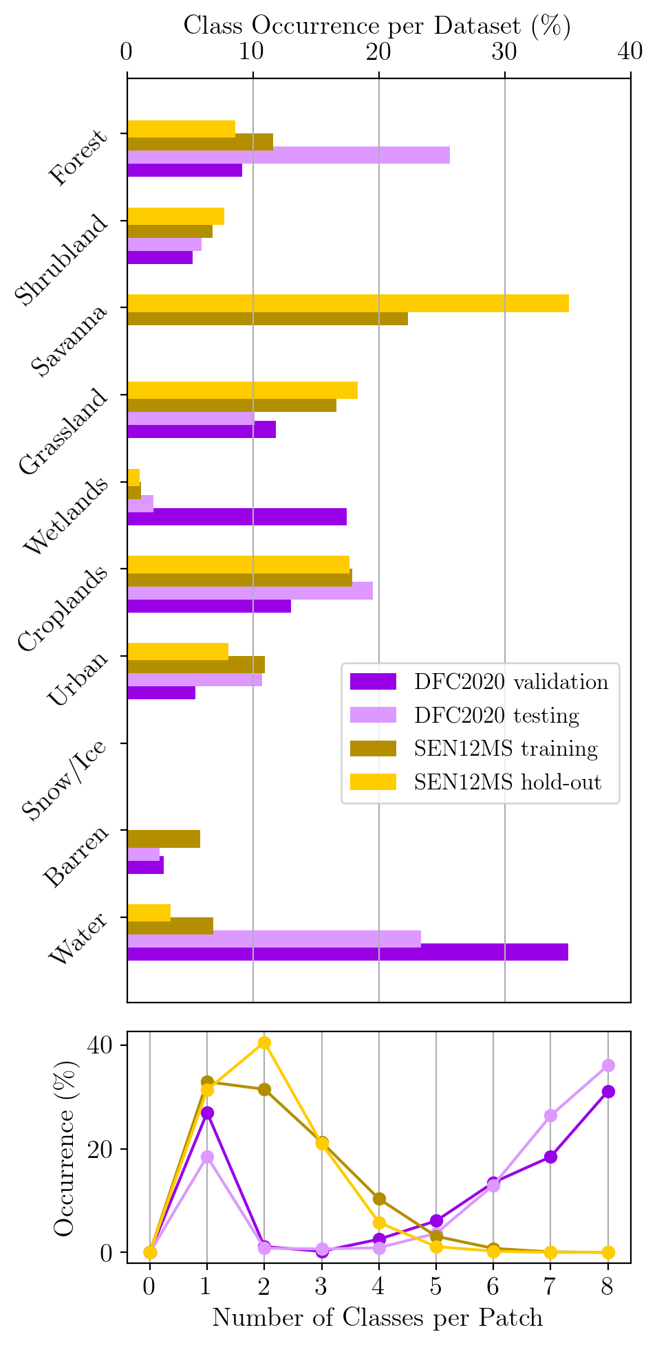
Figure 2: The distribution for the different land cover classes (top) as well as the number of different classes per $256\times 256$-pixels image patch (bottom).

The reason for this imbalancing are multifaceted: Firstly, wetlands, for example, are simply relatively rare in reality. Apart from that, water areas were purposefully undersampled because of the simplicity to map them, whereas urban areas were purposefully oversampled because of their heterogeneity and also their importance to geographical science. As discussed in Section 3.1, the Savanna class is over-represented because the global, MODIS-derived IGBP land cover map, which constitutes the basis of the SEN12MS land cover annotations, contains much more savanna areas than one would expect. This has to be considered when using the dataset as basis for the development of land cover-oriented semantic segmentation models.

3.3 DFC2020

For the IEEE-GRSS 2020 Data Fusion Contest, a high-resolution (GSD: $10$m) dataset for validation and testing was generated in a semi-manual manner, following the simplified IGBP scheme as well. While the DFC2020 validaton and test labels and all relevant meta-information will only officially be published after the end of the contest in April 2020, the class distributions of the data are already shown in Fig. 2 for sake of comparison with SEN12MS. It can be seen that the distributions are fairly similar. The most important exception is the complete absence of the Savanna class. This is due to the fact that the DFC2020 maps were created in a semi-manual manner and on a pixel-level basis for regions of interest outside the typical savanna regions. Besides the absence of the Savanna class, also no Snow/Ice pixels exist in the DFC2020 data.

As can be seen from Fig. 2, another interesting difference between the SEN12MS and the DFC2020 datasets is the fact that the high-resolution DFC2020 patches either contain a single class (e.g. in homogeneous Forest or Water areas) – or more than five classes, whereas the low-resolution MODIS-derived labels of SEN12MS mostly contain one to three classes. This is a clear hint towards the significant resolution difference.

3.4 Predicting High-Resolution Land Cover from Low-Resolution Labels

With the availability of SEN12MS for training and DFC2020 for validation and/or testing, a wide range of possibilities for weakly supervised training of high-resolution land cover prediction models opens up. To make full use of them it is crucial to have a common understanding of the data structures. A summary is given in Tab. 2.

Dataset	Size	Comment
SEN12MS training	$162{,}556$	subset of SEN12MS dedicated to training
SEN12MS hold-out	$18{,}106$	hold-out set with low-res labels; similar spatial and temporal distribution as the overall dataset; used for validation or testing
DFC2020 validation	$986$	used for testing in the first phase of DFC2020, and for validation in the second phase
DFC2020 testing	$5{,}128$	used for testing in the second phase of DFC2020

Table 2: The different sub-datasets that can be built from the SEN12MS and DFC2020 data.

While it is perfectly possible to keep all $180{,}662$ patches of SEN12MS in a single dataset purely used for training, and all $6{,}114$ patches of DFC2020 in another dataset purely used for testing, we suggest to make use of the splits proposed in this paper in future work to ensure comparability between achieved results in a benchmarking sense. The list of hold-out scenes for SEN12MS can be found in the SEN12MS support repository at https://github.com/schmitt-muc/SEN12MS, and the DFC2020 data is provided in separate validation and test packages at https://ieee-dataport.org/competitions/2020-ieee-grss-data-fusion-contest.

4 Baseline Results

To provide a first intuition about what is possible when using the SEN12MS and DFC2020 datasets for weakly supervised learning, first results are collected in this section. They shall also serve as examples for future benchmarking purposes. While land cover maps are traditionally assessed via the overall accuracy (OA) measure, we propose to use the less optimistic average accuracy (AA) for comparison, as it gives less weight to large classes, which are rather simple to classify, e.g. Forest and Water. It is important to note that in this paper, AA refers to average producer’s accuracy, which is highly correlated to the often-used mean intersection over union (mIoU) metric.

To implement the considerations about the difficult Savanna class described in Section 3, during training of all machine learning models, Savanna pixels were not used.

With respect to the satellite input data, the following pre-processing was applied: The Sentinel-1 backscatter values were clipped and normalized to the interval $[-25,0]$, before rescaling to $[0,1]$. In a similar manner, we clipped the intensity values of the Sentinel-2 top-of-atmosphere observations to $[0,10^{4}]$, corresponding to a maximum of $100\%$ surface reflectance before rescaling as well. It is important to note that we made only use of the 10 surface-related Sentinel-2 bands (i.e. the bands with an original resolution of $10$m and $20$m), while the atmosphere-related bands (with an original resolution of $60$m) B1, B9 and B10 were not used.

4.1 Low-Resolution vs. High-Resolution Labels

As a sanity check and the lower end of what is possible, the low-resolution MODIS-derived labels can simply be tested against the high-resolution DFC2020 validation set. The results are shown in the leftmost column of Tab. 3.

Class	LR-HR	DLv3 S2 only	DLv3 S1+S2	Unet S2 only	Unet S1+S2	$k$-means S2 only	$k$-means S1+S2	RF S2 only	RF S1+S2
Forest	51.6%	71.4%	61.2%	67.3%	55.4%	2.4%	1.7%	77.1%	76.9%
Shrubland	7.7%	2.3%	3.8%	0.0%	3.7%	7.7%	5.9%	0.0%	0.0%
Savanna	–	–	–	–	–	–	–	–	–
Grassland	6.7%	64.4%	48.2%	76.7%	77.2%	11.2%	12.5%	90.3%	90.5%
Wetlands	0.6%	2.4%	3.8%	3.7%	3.2%	2.2%	0.3%	4.1%	4.0%
Croplands	64.4%	53.3%	61.9%	65.7%	50.7%	42.1%	13.4%	42.1%	39.6%
Urban	71.5%	71.0%	62.8%	80.9%	73.1%	0.0%	0.0%	0.0%	0.0%
Snow/Ice	–	–	–	–	–	–	–	–	–
Barren	0.3%	0.2%	1.0%	0.6%	0.8%	54.4%	6.2%	0.0%	0.0%
Water	95.1%	88.9%	95.8%	89.4%	92.7%	55.8%	68.9%	25.4%	34.5%
Average	37.2%	44.2%	42.3%	48.1%	44.6%	22.0%	13.6%	29.9%	30.7%

Table 3: Class-wise and average accuracies achieved on the DFC2020 validation dataset for different benchmarks. S2 only indicates that only Sentinel-2 data have been used for the prediction, whereas S1+S2 indicates the case of Sentinel-1/Sentinel-2 data fusion. LR-HR indicates the baseline check of evaluating the MODIS-derived low-resolution labels against the high-resolution DFC2020 reference labels.

While frequent and easy-to-determine classes such as Forest, Urban, and Water show relatively good agreement between the low-resolution labels and the high-resolution reference, less frequent classes, which are harder to identify (e.g. Shrubland, Barren, and Wetlands) cause the average accuracy to drop to a mere $37.2\%$. On the other hand, it seems a bit surprising that the Croplands class also shows a satisfying agreement, although empty fields could certainly be confused with Barren or crops growing up with Grassland. On the opposite, the Grassland class shows an unexpectedly bad accuracy, which is mainly due to a confusion with Shrubland or Wetlands pixels in the high-resolution reference. More details can be seen from the class transition matrix shown in Fig. 3, which depicts the likelihood of a class in the high-resolution DFC2020 data given a class in the low-resolution MODIS-derived land cover map. The good agreement of Forest, Croplands, Urban, and Water are confirmed, while the confusion-prone classes Shrubland, Grassland, Wetlands and Barren can be further interpreted. While the transition of a Wetlands pixel into a Water pixel can be relatively comprehensible, the transition of Barren pixels into Water pixels can be considered a relevant potential source for label noise.

MODIS-derived labels

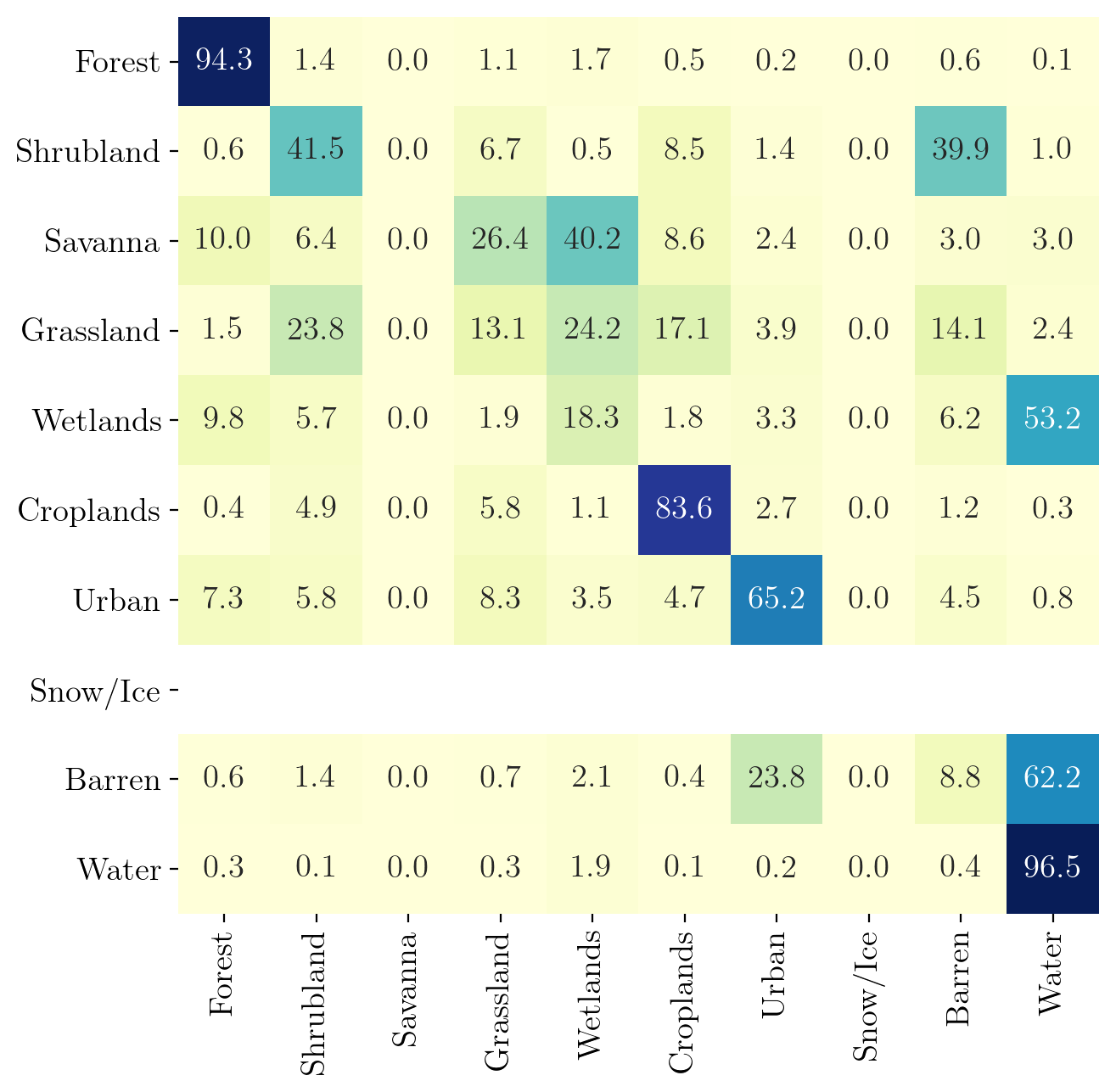
DFC2020 labels

Figure 3: Class transition matrix from low-resolution, MODIS-derived labels to high-resolution DFC2020 labels.

4.2 Off-the-Shelf Models for Semantic Segmentation

To provide a baseline for future developments, Tab. 3 also contains the results for off-the-shelf models for semantic segmentation. All of them were trained on the SEN12MS training subset, validated with the SEN12MS hold-out subset, and tested on the DFC2020 validation set, which was already officially available during the writing of this paper. We implemented the ignoring of the Savanna pixels during training using a masked-cross-entropy loss.

• DeepLabv3+ (DLv3)
  Achieving top-ranking results on various semantic segmentation benchmarks, DeepLabv3+ [Chen et al., 2018] represents a state-of-the-art semantic segmentation architecture and was, thus, used for our baseline experiments. Our implementation used a ResNet-101 backbone with ImageNet pre-trained weights as an initialization. In order for results to be comparable, we fixed the hyperparameters for training. Training was conducted for ten epochs.

• Unet
  In addition to DLv3 we further applied a Unet type architecture [Ronneberger et al., 2015] to the segmentation task. We adopted the last layer to contain nine segmentation maps and masked the loss function to ignore the neglected tenth class. The model contains $\approx 31$ million (random initialized) parameters, and is therefore significantly larger then the DLv3. Another important difference is the utilization of long skip connections in the Unet architecture, which is expected to have a positive influence on preserving fine spatial details.

Our Pytorch-based implementations of the two baseline networks are available at https://github.com/lukasliebel/dfc2020_baseline.

Figure 5 compares how the validation accuracy on the SEN12MS hold-out set and the test accuracy on the DFC2020 validation set change over time for the different models. Since the training is carried out in on the low-resolution MODIS-derived land cover labels without any specific adaptations to cope with the situation of weak supervision, the slightly positive trend of the validation accuracy is not mirrored by the test accuracy – the evolution of the networks remains unstable. In order to fill Tab. 3, we select the checkpoint with the best test accuracy for evaluation. This should be seen as the upper bound of what is achievable with off-the-shelf semantic segmentation networks and does not allow a judgment between the models. The confusion matrix achieved by the best deep semantic segmentation network (i.e. the Unet relying on only Sentinel-2) is shown in Fig. 4.

DFC2020 reference data

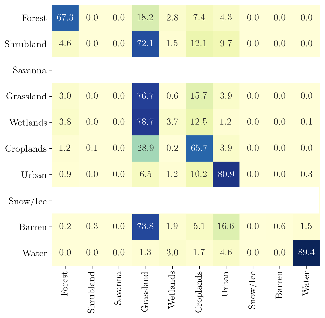
Unet-based predictions

Figure 4: Confusion matrix of the Unet model using only Sentinel-2 data as input.

The results show that even off-the-shelf semantic segmentation models produce results that are significantly better than the low-resolution reference. The most notable improvement is observed for the Grassland class, with also Forest, Croplands, Urban, and Water performing reasonably well. On the downside, Wetlands and Barren are not really mapped well, whereas Shrubland becomes even worse than in the low-resolution input. The main source of confusion is the Grassland class, which collects most predictions from Shrubland, Wetlands and Barren classes. With erroneous Grassland predictions also affecting the Forest, Shrubland and Croplands reference classes, this land cover type will need more attention in future model designs.

Figure 6 provides a visual impression of the mapping quality, taking a prediction example after the first epoch. While the off-the-shelf deep semantic segmentation models are able to recover the general scene structure, fine details get completely lost.

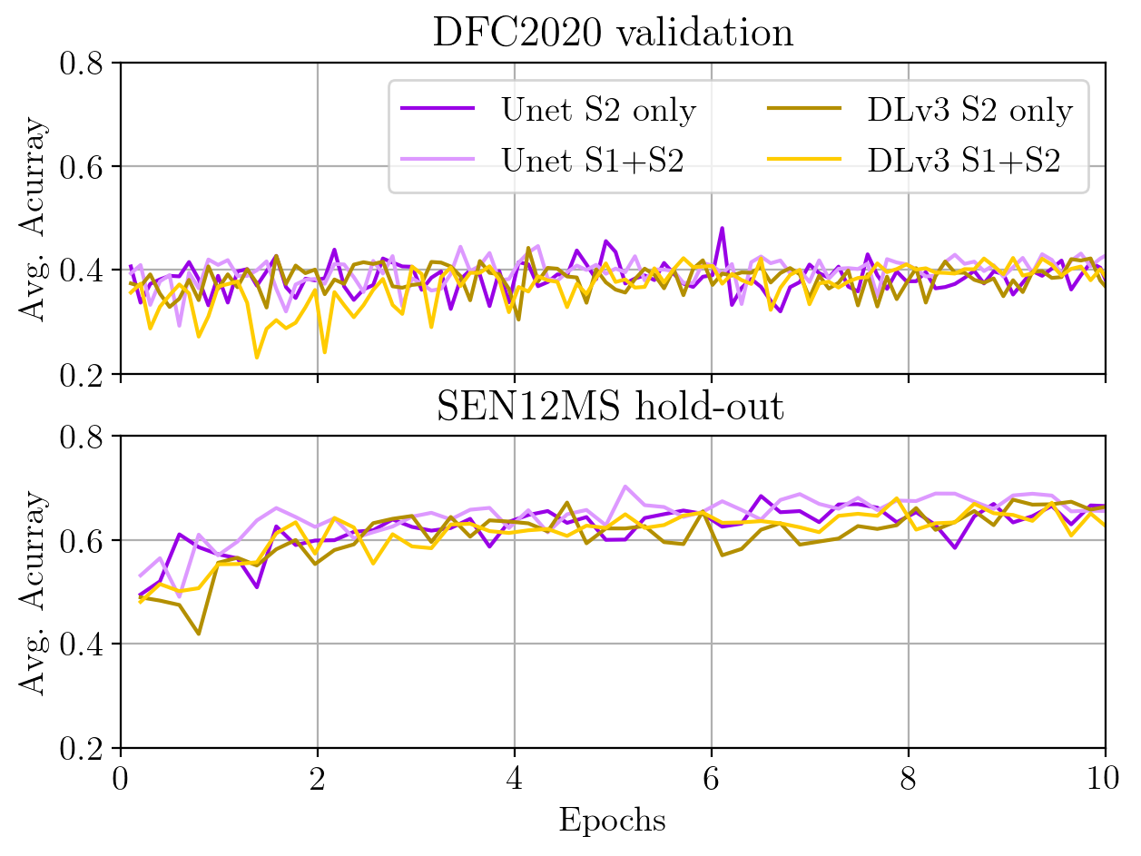
Figure 5: Comparison of the Average Accuracy metric achieved on both the DFC2020 validation as well as the SEN12MS hold-out set over the training process for the different deep semantic segmentation networks described in section 4.2.

4.3 Shallow Learning Baselines

To provide further baselines for the problem at hand, we trained two shallow classifiers – one unsupervised, one supervised – on a subset of the SEN12MS training set. Both classifiers were trained on just $2{,}500$ patches uniformly sub-sampled from the full dataset. Due to the pixel-wise classification approach this amounts to an effective training data set size of about $164$ million individual observations. The sub-sampling is required due to the computational complexity of parts of the training, such as the Kuhn-Munkres algorithm having a run time of $\mathcal{O}(n^{3})$.

Details of the two setups are described in the following. Both used just the above-described 12 channels of Sentinel-1 and Sentinel-2 as pixel-wise input features.

• $k$-means clustering
  $k=8$ clusters, set according to the number of simplified IGBP classes encountered in the sub-sampled training data. The cluster segments are learned completely unsupervised. The re-ordering of cluster labels is done via the Kuhn-Munkres algorithm [Munkres, 1957], with the given low-resolution MODIS-derived labels of the sub-sampled train split serving as a reference. Clustering is done with the best-fitting of 10 $k$-means++ initializations [Arthur, Vassilvitskii, 2007], each fitted for up to 300 iterations.

• Random Forests (RF)
  supervised training on low-resolution MODIS-derived labels of the previously mentioned SEN12MS subset. The model consists of an ensemble of $100$ trees, each with a maximum depth of $10$ nodes.

As can be seen from Tab. 3, shallow classifiers doing simple pixel-wise classification are not capable of reaching the baseline accuracy provided by the low-resolution labels and perform significantly worse than the deep learning models. Interestingly, for $k$-means, a fusion of Sentinel-1 and Sentinel-2 data deteriorates the result, which seems to be mainly caused by the classes Croplands and Barren. Another fact to note is that the predicted maps displayed in Fig. 6 show more spatial details than the results achieved by the deep learning models, albeit at worse semantic accuracy. The existence of some spatial coherence in those pixel-based maps shows that the numerically observed misclassifications are of systematic nature. The Appendix provides supplementary results for weakly supervised learning of shallow classifiers trained directly on the target data, i.e. without spatial generalization.

Sentinel-2 RGB
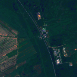
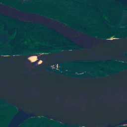
DFC2020 reference
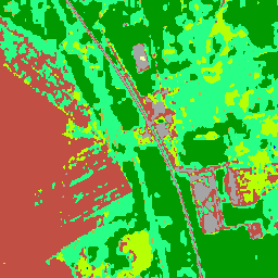
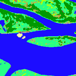
MODIS LC
DLv3
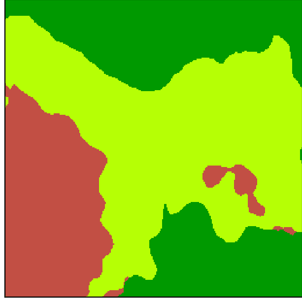
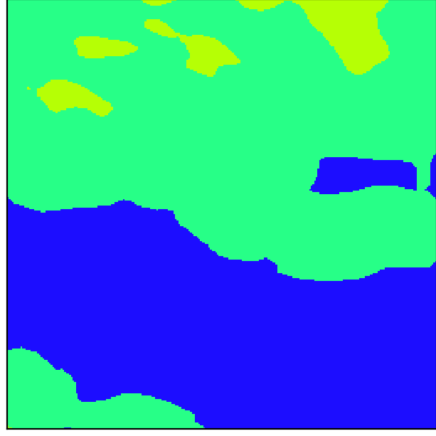
Unet
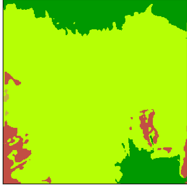
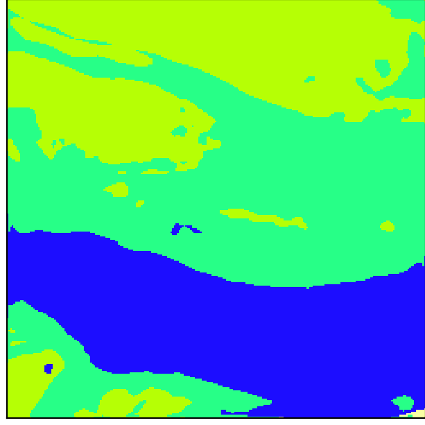
$k$-means
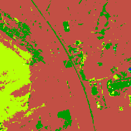
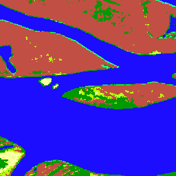
RF

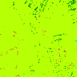
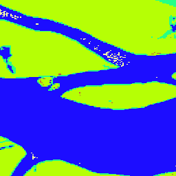
Figure 6: Land cover mapping results achieved with the baseline models for two example patches. Note that for Unet and DLv3 the models based on Sentinel-1 and Sentinel-2 data fusion and achieved after the first training epoch were used to predict the maps shown in this figure, as they provided a visual upper bound.

4.4 Data Fusion

All machine learning models have used either the ten surface-related bands of Sentinel-2 as input, or have relied on a form of early data fusion by combining this Sentinel-2 input with the two polarimetric channels of Sentinel-1. As can be seen from Tab. 3, the fusion of Sentinel-1 and Sentinel-2 data only leads to slightly better results than what is achievable if only Sentinel-2 is used in the RF case. The fact that the fusion doesn’t seem to help to improve the metrics achieved with the deep learning models should not be misunderstood: Since Tab. 3 collects the best validation results, a fair comparison among the four deep semantic segmentation setups is not ensured. However, it will certainly be necessary to develop more sophisticated fusion procedures than simple band concatenation, e.g. with sub-networks that take the different data peculiarities into account as, e.g. proposed in [Gawlikowski et al., 2020].

5 Discussion

The baseline results presented in Section 4 show that mapping land cover on a global scale with models learned on inaccurate and inexact training labels remains an exciting challenge.

In particular, it is interesting to note that three classes get consistently bad metrics throughout all classification methods (cf. Tab. 3): Shrublands, Wetlands and Barren. As can be seen in Fig. 2, those three classes are the least frequent in the SEN12MS dataset (except the understandably rare Snow/Ice class). On the other hand, Wetlands are massively over-represented in the DFC2020 validation set.

Figure 3 shows that all three problematic classes seem to be significantly mislabeled in the low-resolution land cover maps – while Wetlands and Barren areas used to label pixels actually containing water, Shrubland pixels often are represented as Barren in he high-resolution reference.

Finally, it seems very promising that the Grassland class is apparently not well represented by the low-resolution MODIS-derived labels, but can be well predicted by most models besides the unsupervised $k$-means. This indicates the potential of the topic addressed in this paper.

All in all, it becomes apparent that good models would have to solve two challenges: The transfer of spatial information from the training data sampled by the SEN12MS dataset to the location of interest; and the transfer of land cover annotations from low resolution and noisy quality to high resolution and better quality. Standard methods without dedicated adaptations are apparently limited in their capabilities to do so.

6 Summary & Conclusion

In this paper, we have used the SEN12MS dataset and the data provided in the frame of the IEEE-GRSS 2020 Data Fusion Contest to address the challenge of learning semantic segmentation models for global land cover mapping from inaccurate and inexact labels. While standard shallow and deep learning approaches were shown to already provide promising mapping capabilities, the results are not satisfying enough yet to consider off-the-shelf approaches for operational solutions. Therefore, we argue that specific models from the field of weakly supervised machine learning must be developed and expect that they will contribute greatly to a regular and fully automatic satellite-based monitoring of global land cover.

APPENDIX: Weakly Supervised Learning Without Spatial Generalization

Of course, the question may arise whether the problem of weakly supervised learning for semantic segmentation of satellite images for land cover mapping could be simplified by aiming at less generic models. One way to create a less generic model is to forgo the desire to encode spatial generalization required by a globally applicable model and to train a scene-dependent model instead. To provide a sanity check, we have trained the shallow classifiers described in Section 4.3 not on any data of the SEN12MS dataset, but only on the low-resolution labels included in the DFC2020 validation set. This follows the rationale that such labels are available for every location on the globe. The results are depicted in Tab. 4 and Fig. 7. It can be seen that these results exceed the quality of the results achieved for the scene-agnostic models, even though only shallow classifiers and only $986$ training samples were used. Apparently, transferring noisy, low-resolution labels into more accurate, high-resolution labels is a much simpler task than transferring land cover labels from one region of the globe to another region.

Class	$k$-means S2 only	$k$-means S1+S2	RF S2 only	RF S1+S2
Forest	80.7%	93.3%	80.1%	80.1%
Shrubland	0.3%	44.7%	0.9%	0.8%
Savanna	–	–	–	–
Grassland	21.2%	49.8%	78.0%	78.2%
Wetlands	38.2%	1.3%	0.0%	0.0%
Croplands	33.4%	40.3%	80.7%	80.9%
Urban	38.8%	50.7%	91.8%	91.7%
Snow/Ice	–	–	–	–
Barren	0.4%	9.8%	0.0%	0.0%
Water	73.1%	48.7%	99.9%	99.8%
Average	35.8%	42.3%	54.0%	54.1%

Table 4: Quantitative results achieved on the DFC2020 validation dataset for the shallow classifiers trained on the low-resolution labels of the DFC2020 validation set.

$k$-means
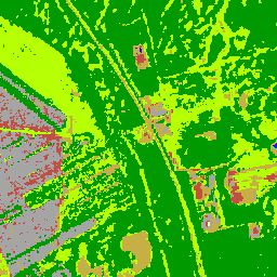
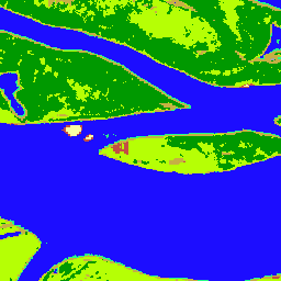
RF

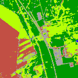
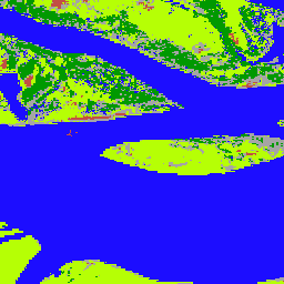
Figure 7: Qualitative results achieved with the shallow classifiers trained on the low-resolution labels of the DFC2020 validation set.

References

- [Arthur, Vassilvitskii, 2007] Arthur, D., Vassilvitskii, S., 2007. k-means++: The advantages of careful seeding. Proc. ACM-SIAM Symp. on Discrete Algorithms, 1027–1035.
- [Chen et al., 2018] Chen, L.-C., Zhu, Y., Papandreou, G., Schroff, F., Adam, H., 2018. Encoder-decoder with atrous separable convolution for semantic image segmentation. Proc. ECCV, 801–818.
- [Chi et al., 2016] Chi, M., Plaza, A., Benediktsson, J. A., Sun, Z., Shen, J., Zhu, Y., 2016. Big data for remote Sensing: challenges and opportunities. Proc. IEEE, 104(11), 2207-2219.
- [Cihlar, 2000] Cihlar, J., 2000. Land cover mapping of large areas from satellites: status and research priorities. Int. J. Remote Sens., 21(6-7), 1093–1114.
- [Drusch et al., 2012] Drusch, M., Del Bello, U., Carlier, S., Colin, O., Fernandez, V. et al., 2012. Sentinel-2: ESA’s optical high-resolution mission for GMES operational services. Remote Sens. Environ., 120, 25-36.
- [Frenay, Verleysen, 2014] Frenay, B., Verleysen, M., 2014. Classification in the presence of label noise: a survey. IEEE Trans. Neural Netw. Learn. Syst, 25(5), 845-869.
- [Fu et al., 2018] Fu, K., Lu, W., Diao, W., Yan, M., Sun, H. et al., 2018. WSF-NET: weakly supervised feature-fusion network for binary segmentation in remote sensing image. Remote Sens., 10(12), 1970.
- [Gawlikowski et al., 2020] Gawlikowski, J., Schmitt, M., Kruspe, A., Zhu, X. X., 2020. On the fusion strategies of Sentinel-1 and Sentinel-2 data for local climate zone classification. Proc. IGARSS.
- [Ghosh et al., 2017] Ghosh, A., Kumar, H., Sastry, P. S., 2017. Robust loss functions under label noise for deep neural networks. Proc. AAAI.
- [Gong et al., 2019] Gong, P., Liu, H., Zhang, M., Li, C., Wang, J. et al., 2019. Stable classification with limited sample: transferring a 30-m resolution sample set collected in 2015 to mapping 10-m resolution global land cover in 2017. Science Bulletin, 64(6), 370-373.
- [Grekousis et al., 2015] Grekousis, G., Mountrakis, G., Kavouras, M., 2015. An overview of 21 global and 43 regional land-cover mapping products. Int. J. Remote Sens., 36(21), 5309-5335.
- [Kellenberger et al., 2019] Kellenberger, B., Marcos, D., Tuia, D., 2019. When a few clicks make all the difference: improving weakly-supervised wildlife detection in UAV images. Proc. CVPRW.
- [Loveland, Belward, 1997] Loveland, T., Belward, A., 1997. The international geosphere biosphere programme data and information system global land cover data set (DISCover). Acta Astronautica, 41(4-10), 681–689.
- [Malkin et al., 2019] Malkin, K., Robinson, C., Hou, L., Soobitsky, R., Czawlytko, J. et al., 2019. Label super-resolution networks. Proc. ICLR.
- [Munkres, 1957] Munkres, J., 1957. Algorithms for the assignment and transportation problems. J. Soc. Ind. Appl. Math., 5(1), 32-39.
- [Reed et al., 2015] Reed, S., Lee, H., Anguelov, D., Szegedy, C., Erhan, D., Rabinovich, A., 2015. Training deep neural networks on noisy labels with bootstrapping. arXiv:1412.6596.
- [Reichstein et al., 2019] Reichstein, M., Camps-Valls, G., Stevens, B., Jung, M., Denzler, J. et al., 2019. Deep learning and process understanding for data-driven Earth system science. Nature, 566, 195-204.
- [Robinson et al., 2019] Robinson, C., Hou, L., Malkin, K., Soobitsky, R., Czawlytko, J. et al., 2019. Large scale high-resolution land cover mapping with multi-resolution data. Proc. CVPR, 12726–12735.
- [Rolnick et al., 2018] Rolnick, D., Veit, A., Belongie, S., Shavit, N., 2018. Deep learning is robust to massive label noise. arXiv:1705.10694.
- [Ronneberger et al., 2015] Ronneberger, O., Fischer, P., Brox, T., 2015. U-net: Convolutional networks for biomedical image segmentation. Proc. MICCAI, 234–241.
- [Schmitt et al., 2019] Schmitt, M., Hughes, L. H., Qiu, C., Zhu, X. X., 2019. SEN12MS – a curated dataset of georeferenced multi-spectral Sentinel-1/2 imagery for deep learning and data fusion. ISPRS Ann. Photogramm. Remote Sens. Spatial Inf. Sci., IV-2/W7, 153–160.
- [Sukhbaatar et al., 2015] Sukhbaatar, S., Bruna, J., Paluri, M., Bourdev, L., Fergus, R., 2015. Training convolutional networks with noisy labels. arXiv:1406.2080.
- [Torres et al., 2012] Torres, R., Snoeij, P., Geudtner, D., Bibby, D., Davidson, M. et al., 2012. GMES Sentinel-1 mission. Remote Sens. Environ., 120, 9-24.
- [Wang et al., 2020] Wang, S., Chen, W., Xie, S. M., Azzari, G., Lobell, D. B., 2020. Weakly supervised deep learning for segmentation of remote sensing imagery. Remote Sens., 12(2), 207.
- [Yokoya et al., 2020] Yokoya, N., Ghamisi, P., Hänsch, R., Schmitt, M., 2020. 2020 IEEE GRSS Data Fusion Contest: Global Land Cover Mapping with Weak Supervision. IEEE Geosci. Remote Sens. Mag., 8(1), 154-157.
- [Zhang et al., 2015] Zhang, D., Han, J., Cheng, G., Liu, Z., Bu, S., Guo, L., 2015. Weakly supervised learning for target detection in remote sensing images. IEEE Geosci. Remote Sens. Lett., 12(4), 701-705.
- [Zhou, 2018] Zhou, Z. H., 2018. A brief introduction to weakly supervised learning. National Science Review, 5(1), 44–53.
- [Zhu, Goldberg, 2009] Zhu, X., Goldberg, A. B., 2009. Introduction to semi-supervised learning. Synthesis lectures on artificial intelligence and machine learning, Morgan & Claypool.
- [Zhu et al., 2017] Zhu, X. X., Tuia, D., Mou, L., Xia, G., Zhang, L. et al., 2017. Deep Learning in Remote Sensing: A Comprehensive Review and List of Resources. IEEE Geosci. Remote Sens. Mag., 5(4), 8-36.