Phase-controllable Nonlocal Spin Polarization in Proximitized Nanowires

Abstract

We study the magnetic and superconducting proximity effects in a semiconducting nanowire (NW) attached to superconducting leads and a ferromagnetic insulator (FI). We show that a sizable equilibrium spin polarization arises in the NW due to the interplay between the superconducting correlations and the exchange field in the FI. The resulting magnetization has a nonlocal contribution that spreads in the NW over the superconducting coherence length and is opposite in sign to the local spin polarization induced by the magnetic proximity effect in the normal state. For a Josephson-junction setup, we show that the nonlocal magnetization can be controlled by the superconducting phase bias across the junction. Our findings are relevant for the implementation of Majorana bound states in state-of-the-art hybrid structures.

Semiconducting nanowires (NWs) in proximity with superconductors (SCs) are central to the creation of a topologically non-trivial superconducting state, which manifests itself through Majorana zero modes at the edges of the NW Lutchyn et al. (2010); Oreg et al. (2010); Mourik et al. (2012); Rokhinson et al. (2012); Das et al. (2012); Finck et al. (2013); Albrecht et al. (2016); Deng et al. (2016); Suominen et al. (2017); Nichele et al. (2017); Takei et al. (2013); Chang et al. (2015); Lutchyn et al. (2011). The basic ingredients needed for the topological phase are the spin-orbit interaction (SOI), superconducting correlations, and Zeeman splitting Qi and Zhang (2011); Elliott and Franz (2015); Beenakker (2013); Alicea (2012); Lutchyn et al. (2018); Sarma et al. (2015); Stanescu and Tewari (2013). Whereas SOI and superconductivity are intrinsic properties of the materials, the Zeeman splitting is usually generated by applying a rather large magnetic field Lutchyn et al. (2010); Oreg et al. (2010), which introduces technical limitations on the use of superconducting elements.

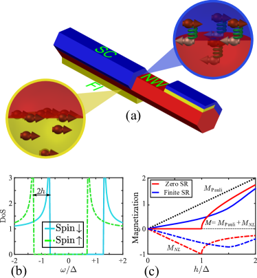
Figure 1: (Color online.) (a) Sketch of a nanowire (NW) in proximity with superconductors (SCs) and ferromagnetic insulators (FIs). (b) Spin-resolved density of state (DoS) of a spin-split SC. (c) Magnetizations induced in a SC in an homogeneous Zeeman field $h$. The dot black line describes Pauli magnetization, $M_{\textrm{Pauli}}$ and the solid lines plot the total magnetization, $M$ for zero (red) and finite (blue) spin relaxation (SR). The dashed lines show the nonlocal magnetization, $M_{NL}$ given by the difference between $M$ and $M_{\textrm{Pauli}}$, displayed for zero (red) and finite (blue) SR.

Alternatively, such a spin splitting can be generated without applying an external field by the magnetic proximity effect from a magnetic insulator  Bergeret et al. (2018); Giazotto and Taddei (2008); Yang et al. (2013); Eremeev et al. (2013); Virtanen et al. (2018); Wei et al. (2016); Katmis et al. (2016). Indeed, a Zeeman-like splitting at zero magnetic field has been observed in superconducting Al layers in contact with the ferromagnetic insulator (FI) EuS Hao et al. (1991); Meservey et al. (1970); Hao et al. (1990); Strambini et al. (2017); Moodera et al. (1988); Rouco et al. (2019). A recent article reports the first hybrid epitaxial growth of InAs NWs in proximity with EuS and Al Liu et al. (2019). Even though the experiment is inconclusive with regard to Majorana physics, the NWs show signs of coexisting proximity-induced superconducting gap and spin splitting. These proximitized NWs are pivotal in the study of the topological superconductivity Sau et al. (2010); Lee et al. (2012); Livanas et al. (2019).

Motivated by this recent experiment Liu et al. (2019), we study theoretically a multiband NW in the diffusive regime proximitized by FIs and SCs, see sketch in Fig. 1(a). We show that, apart from the local spin polarization induced by the FI, a nonlocal electronic spin polarization emerges in the NW as a result of an interplay between the magnetic and superconducting proximity effects. The magnetic proximity effect takes place at the FI/NW interface, where the conduction electrons in the NW interact with the local moments of the FI via the spin-exchange coupling. This interaction leads to a Pauli paramagnetic response of the conduction electrons, which is manifested as a locally induced magnetization in the NW at the FI. In addition, the superconducting proximity effect at the NW/SC interface allows for a leakage of Cooper-pair correlations into the NW. The Cooper pairs become polarized by the FI exchange field, admixing to the usual singlet pairing a triplet component of the superconducting correlations. As a result, the Pauli paramagnetic response at the NW/FI interface becomes screened by a spin polarization, which spreads in the NW over large distances, on the order of the superconducting coherence length. This long-ranged component of magnetization is opposite in sign to the Pauli magnetization and its strength is proportional to the condensate density in the NW. In this letter, we calculate this nonlocal magnetization as a function of the system parameters, demonstrate its control by the phase difference in a loop geometry, and propose a way of measuring it via spin-dependent spectroscopy.

It is illustrative to review the response of a conventional SC to a Zeeman or exchange field $h(\boldsymbol{r})$ Abrikosov and Gor?kov (1962); Larkin and Varlamov (2005); Fulde and Ferrell (1964). In normal state, the response is local and leads to a Pauli magnetization $M_{\textrm{Pauli}}(\boldsymbol{r})=g\mu_{B}\nu_{F}h(\boldsymbol{r})$, dot-black curve in Fig. 1(c). Here, $g$ is g-factor, $\mu_{B}$ is Bohr magneton, and $\nu_{F}$ is the normal density of states (DoS) at the Fermi level for each spin. When the temperature, $T$ is below the critical superconducting temperature, there exists an additional nonlocal contribution to magnetization, $M_{NL}(\boldsymbol{r})$ (dashed-red curve in Fig. 1c), from the superconducting condensate. In a homogeneous SC at zero temperature, this contribution exactly compensates the Pauli one, $M_{NL}=-M_{\textrm{Pauli}}$, for fields $h$ smaller than the superconducting gap, $\Delta$. This explains the zero magnetic susceptibility of a SC Yosida (1958). In the presence of a spin relaxation (SR), the full magnetization cancellation fails, according to Abrikosov and Gorkov’s theory of the Knight shift in SCs Abrikosov and Gor?kov (1962). In Fig. 1(c), we include the SR due to the SOI and static disorder (blue curves). For $h>\Delta$, the compensation is incomplete and the total magnetization reads $M=M_{\textrm{Pauli}}\sqrt{h^{2}-\Delta^{2}}/h$ Bergeret et al. (2005); Karchev et al. (2001); Shen et al. (2003). One can draw a connection between the nonlocal magnetization and the modified spectrum of the SC (Fig. 1b). The exchange field $h$ leads to both a splitting of the quasi-particle DoS and a reduction of the superconducting gap. As far as the latter is finite, the total magnetization is zero. For $h>\Delta$, the gap closes and a finite magnetization appears as a consequence of an incomplete compensation $|M_{NL}|<M_{\textrm{Pauli}}$. The previous discussion has been introduced for pedagogical purposes, as it is useful when presenting our main results .

We now focus on an inhomogeneous system, as shown in Fig. 1(a). It consists of a NW in contact with SCs and FIs. To describe the superconducting proximity effect, we use the quasiclassical equations and assume the diffusive regime in the NW. The characteristic length over which the Cooper-pair correlations decay in the NW is denoted as $\xi_{N}$. To describe the magnetic proximity effect in the FI/NW interface, we follow the approach of Ref. Zhang et al. (2019) and assume a region of thickness $b$ where the local magnetic moments of FI and the itinerant electrons of NW interact via a spin-exchange coupling. This interaction leads to an interfacial exchange field $h_{ex}$ acting on the itinerant electrons. Because $b\ll\xi_{N}$, the exchange field can be described in the quasiclassical equations by $h_{b}(y)=h_{ex}b\delta(y)$, where we denote with $y$ the coordinate axis perpendicular to the FI/NW interface Bergeret et al. (2000). At this stage we can already anticipate the appearance of a nonlocal magnetization in opposite direction to the one localized at the FI/NW interface. The Cooper pairs in the NW consist of electrons with opposite spins (singlet state). Energetically it is favorable that one electron of the pair with spin parallel to the local exchange localizes at the interface, while the another with opposite spin remains in the NW. Thus, a nonlocal magnetization opposite to the interfacial one, is induced in the NW and extends over the characteristic Cooper size, $\xi_{N}$. This physical picture resembles the inverse proximity effect in metallic superconductor-ferromagnetic junctions predicted in Refs. Bergeret et al. (2004a, b); Dahir et al. (2019) and experimentally verified in Refs. Xia et al. (2009); Salikhov et al. (2009a, b).

To quantify this effect we calculate the nonlocal electronic equilibrium spin polarization, $M_{NL}$, induced in the NW. This is given by

$$\frac{M_{NL}(X)}{g\mu_{B}\nu_{F}}=\frac{1}{2}\int^{+\infty}_{-\infty}d\omega f(\omega)[N^{\uparrow}(\omega,X)-N^{\downarrow}(\omega,X)],$$ (1)

where $f(\omega)=1/(e^{\omega/T}+1)$ is equilibrium Fermi distribution function, and $N^{\uparrow/\downarrow}(\omega,X)$, are the local DoS for spin-up and -down electrons. The exchange field at the FI/NW leads to $N^{\uparrow}\neq N^{\downarrow}$ and hence to a finite $M_{NL}$. In addition to the nonlocal term there is the Pauli magnetization localized at the FI/NW interface $M_{\textrm{Pauli}}=g\mu_{B}\nu_{F}h_{ex}b\delta(y)$. Thus, the total magnetization equals $M_{\textrm{Pauli}}+M_{NL}$.

We consider first the SC/NW-FI/SC setup sketched in the inset of Fig. 2(c). The NW is in contact with a FI, and sandwiched between two SCs. The phase difference between the SCs, $\phi$, can be tuned by a magnetic flux, when the junction is part of a superconducting loop. We assume a diffusive NW in order to use the well-established Usadel equationUsadel (1970). In this respect, our results apply straightforwardly to metallic NW like Cu. In semiconducting NWs, the degree of disorder depends on doping. For example, the InAs wires studied in the experiments of Refs. Giazotto et al. (2011); Tiira et al. (2017); Iorio et al. (2018); Strambini et al. (2020) are in a metallic regime and are good candidates for the verification of our predictions. We denote with $x$ the axis of the NW of length $L_{N}$. The NW-FI interface is orthogonal to the $y$-axis and the NW width in this direction is $W_{N}$. In this first example we assume that $W_{N},L_{N}\ll\xi_{N}$ and integrate the quasiclassical equations over the volume of the NW. The integration in $y$ direction results in an effective exchange field $h_{F}=h_{ex}b/W_{N}$, whereas the integration over $x$ can be performed with help of the Kupriyanov-Lukichev boundary conditions Kuprianov and Lukichev (1988) and accounts for the superconducting proximity effect. In this way we obtain a compact expression for the DoS SM :

$$N^{\eta}(\omega)=\left|\mathrm{Re}\left\{\frac{\omega_{r}+\eta h_{F}}{\sqrt{\left(\omega_{r}+\eta h_{F}\right)^{2}-\left(\Delta_{r}\right)^{2}}}\right\}\right|,$$ (2)

where $\eta=\pm 1$ for spin $\uparrow$/$\downarrow$. This expression has the same structure as the BCS DoS of a spin-split superconductor with renormalized frequency, $\omega_{r}=\omega+2i\epsilon_{b}\mathcal{G}_{S}$ and order parameter $\Delta_{r}=2\epsilon_{b}\cos(\phi/2)\mathcal{F}_{S}$, where $\mathcal{G}_{S}=-i\omega/\sqrt{\Delta^{2}-\omega^{2}}$, $\mathcal{F}_{S}=\Delta/\sqrt{\Delta^{2}-\omega^{2}}$. $\epsilon_{b}=D/(L_{N}\sigma_{N}R_{\square})$ is an energy proportional to the tunneling rate across the NW/SC interface, where $R_{\square}$ is the interface resistance per area, $D$ is the diffusion coefficient, and $\sigma_{N}$ is the conductivity of the NW. Equation (2) is the generalization of the short-junction limit expression for the DoS Seviour and Volkov (2000); Börlin et al. (2002); Bezuglyi et al. (2011) in the presence of a FI. With its help we provide below a clear physical picture of the main effect by making a connection between the spectrum of the junction and the spectral properties of the bulk system.

From Eq. (2), one can calculate the gap induced in the NW by the superconducting proximity effect. In the limit of transparent contact, $\epsilon_{b}\gg\Delta$, this gap is of the same order as the SC gap and the spin splitting is negligibly small. In the case of a finite NW/SC barrier, when $\epsilon_{b}\ll\Delta$, Eq. (2) describes a NW with an induced minigap, $\Delta_{N}=\Delta^{0}_{N}\cos(\phi/2)$, with $\Delta^{0}_{N}=2\epsilon_{b}$, and a spin splitting in the DoS due to the effective exchange field, $h_{F}$. 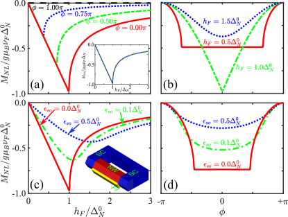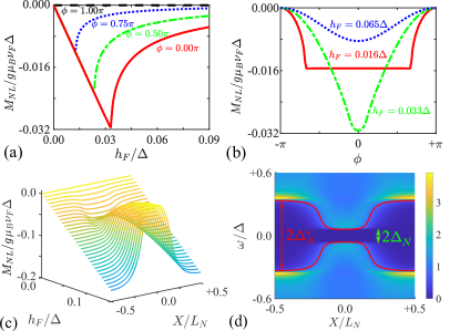In all cases the minigap induced in the NW is maximum when $\phi=0$ and vanishes at $\phi=\pi$. By substituting Eq. (2) into Eq. (1), we obtain the nonlocal magnetization, $M_{NL}$ plotted in Fig. 2. As far as $h_{F}<\Delta_{N}$, nonlocal magnetic moments, $M_{NL}W_{N}A$ compensates the Pauli ones, $\int_{b}M_{\textrm{Pauli}}=g\mu_{B}\nu_{F}h_{ex}bA$ localized at the FI/NW interface, with $A$ being the area of FI/NW interface. At $h_{F}=\Delta_{N}$, $M_{NL}$ reaches a maximum value, $g\mu_{B}\nu_{F}\Delta_{N}$ and decays as $h_{F}-\sqrt{h_{F}^{2}-\Delta_{N}^{2}}$ for $h_{F}>\Delta_{N}$ Bergeret et al. (2005); Karchev et al. (2001); Shen et al. (2003). This is the same behaviour as the bulk superconductor discussed in Fig. 1(c), after identifying $\Delta$ and $h$ with the induced minigap $\Delta_{N}$ and effective exchange field $h_{F}$, respectively. This analogy is clearly seen if we plot the curves of Fig. 2(a) as a function $h_{F}/\Delta_{N}$. In this case all curves collapse into one (inset of Fig. 2a) coinciding with the behaviour shown in Fig. 1(c). In Fig. 2(b) we show the dependence of $M_{NL}$ on the phase difference $\phi$ for different values of $h_{F}$. When $h_{F}\leq\Delta_{N}^{0}$, $M_{NL}$ remains constant for all phases smaller than $\arccos{h_{F}/\Delta_{N}^{0}}$ (red curve in Fig. 2b). In other words, as far as $h_{F}$ is smaller than the induced gap $\Delta_{N}=\Delta_{N}^{0}\cos(\phi/2)$, the $M_{NL}(\phi)$ curve shows a plateau at the value opposite to $M_{\textrm{Pauli}}$. Interestingly, the value of $M_{NL}$ is proportional to the distance between the coherent peaks in the spin-splitting DOS, similar to those shown in Fig. 1(b). Indeed, in the present case when $\Delta_{N}\ll\Delta$, according to Eq. (2), the peaks at positive energies occur at $\omega^{\uparrow,\downarrow}\approx\Delta_{N}(\phi)\pm h_{F}$ SM . The maximum modulation is achieved for $h_{F}=\Delta^{0}_{N}$ (green curve in Fig. 2b) in which the full screening of $M_{NL}$ only occurs at $\phi=0$. For larger values of $h_{F}$, the NW is gapless and $M_{NL}(\phi)$ is overall reduced (blue curve).

In the presence of SOI, electron spin channels are mixed. In this case the DoS of the NW is described by Eq. (2), after replacing $\omega_{r}$ and $\Delta_{r}$ by $\omega^{\eta}_{r}=\omega+i\Delta^{0}_{N}\mathcal{G}_{S}+2i\epsilon_{so}G_{N}^{-\eta}$ and $\Delta^{\eta}_{r}=\Delta_{N}\mathcal{F}_{S}+2\epsilon_{so}F_{N}^{-\eta}$, respectively. Here, $F_{N}^{\eta}$ and $G_{N}^{\eta}$ are the normal and anomalous parts of the retarded Green‘s function of the NW, respectively SM . $\epsilon_{so}$ is the spin-relaxation rate due to SOI. The effect of a finite SR is shown in Fig. 2(c-d). As expected from the analogy with the bulk SC, Fig. 1(c), the main effect of the SR is the uncompensated screening of the Pauli magnetization, $-M_{NL}<M_{\textrm{Pauli}}$, as shown by the green and blue curves in panel 2(c). In addition, the SR leads to a shift of the maximum of the $M_{NL}(h_{F})$ curves towards larger values of $h_{F}$, such that, for $h_{F}>\Delta_{N}$, $M_{NL}$ is enhanced by the SR. This is due to the reduction of the effective exchange field ftw , which results into the right shift of $M_{NL}$ with respect to $h_{F}$ in analogy with the bulk case shown by the dot-dash-blue curve of Fig. 1(c).

Figure 2: (Color online.) Nonlocal magnetization, $M_{NL}$ induced in the NW in a SC/NW-FI/SC setup (see inset of panel (c)). Panels (a,b) show $M_{NL}$ as a function of (a) $h_{F}/\Delta^{0}_{N}$ and (b) $\phi$, respectively, in the absence of SR. Panels (c,d) shows the same dependencies in the presence of SR caused by static disorder and SOI. We have set $\phi=0$ in panel (c) and $h_{F}=0.75\Delta^{0}_{N}$ in panel (d). Other parameters: $T=0$ and $\Delta^{0}_{N}=0.02\Delta$.

So far we have analyzed a short NW sandwiched between two SCs. In a more realistic setup, the length of the NW, $L_{N}$ can be larger than the $\xi_{N}$. Moreover, in typical lateral structures the NW is partially covered by the SCs films of length $L_{S}$. Such a lateral setup is sketched in Fig. 3(a). We assume that the NW is grown on top of a FI substrate, and that its cross-section dimensions are smaller than $\xi_{N}$. In this case one can integrate the Usadel equation over the cross-section and reduce the problem to an effective 1D geometry (details are given in the supplementary material SM ). Hereafter, we assume a symmetric setup with $L_{S}=L_{N}/3$ and $L_{F}=L_{N}$ (other situations are analyzed in the Ref. SM ), such that the distance between the SCs is $L=L_{N}/3$, and solve the Usadel equation numerically. We neglect the effect of SOI. This is a good approximation if the NM is a metal such as Cu, for which the SR rate is much smaller than the gapVillamor et al. (2013). But also in InAs, the typical SR time is $\tau_{s}\simeq 0.02-1.00$ ns Murzyn et al. (2003); Song and Kim (2002); Murdin et al. (2005), which corresponds to $\epsilon_{so}=\hbar/\tau_{s}\simeq 1-30\mu$eV. Whereas the induced gap may reach 150 $\mu$eV or even larger Chang et al. (2015); Kjærgaard et al. (2016), such that the ratio $\epsilon_{so}/\Delta<1$.

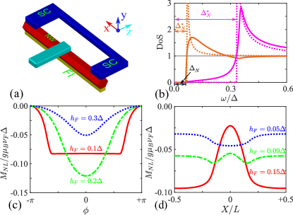
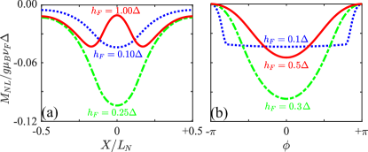
Once induced, the minigap is constant in all the NWLe Sueur et al. (2008). Its value depends on the distance between the superconducting electrodes and the characteristic barrier energy $\epsilon_{b}=D/(W_{N}R_{\square}\sigma_{N})$. In the short limit, $L_{N}\ll\xi_{N}$, $M_{NL}$ is almost constant in the NW and the results are similar to those shown in Figs. 2(a) and (b) SM . More interesting is the case when $L_{N}$ is of the order of $\xi_{N}$. Numerical results of the spatial dependence $M_{NL}(X)$ for $L_{N}=4.7\xi_{0}$ and different values of $h_{F}$, are shown in Fig. 3(d). Remarkably, the shape of the $M_{NL}(X)$ curve depends on the strength of $h_{F}$. These different behaviours can be explained in light of Eq. (1). The integrand in this expression can be well approximated by replacing the exact DoS, $N(\omega,X)$ by a BCS-like one, $N_{BCS}(\omega,\Delta^{*}_{N}(X))$ with a position-dependent pseudogap $\Delta^{*}_{N}(X)$, defined as the energy where $N(\omega)$ intersects with the one in the normal state $N_{0}(\omega)=1$, as shown in Fig. 3(b). Whereas the real minigap, $\Delta_{N}$, is position independent, $\Delta^{*}_{N}$ is not. In fact, the pseudogap is smaller in the middle of the wire becoming larger in the regions below the SCs (see also Fig. 2d in Ref. SM ). The shape of the $M_{NL}(X)$ is determined by the ration $h_{F}/\Delta^{*}_{N}(X)$, in the same way as in the short junction limit $h_{F}/\Delta^{0}_{N}$ determines $M_{N}$, see Figs. 2 (a,c). Indeed, for a given $h_{F}$ with $h_{F}<\Delta^{*}_{N}(X)$ for all $X$, the values of $|M_{NL}|$ increases towards the middle of the wire (blue curve in Fig. 3(d)). In contrast, if $\Delta^{*}(-L/2)>h_{F}>\Delta^{*}(0)$ then a double-minima curve is obtained (green curve). Larger values of $h_{F}$ leads to $|M_{N}(X)|$ with a minimun at $X=0$ (red curve). The actual shape of the curve can be inferred from the $X$ dependence of $\Delta^{*}$ which is shown in Fig. 2c in Ref. SM . Finally, Fig. 3(c) shows the phase dependence of $M_{NL}$ calculated in the center of the wire for different values of $h_{F}$. The result at low temperatures is qualitatively similar to the one obtained for the simpler setup analyzed in Fig. 2(b): for values of $h_{F}$ smaller than the pseudogap $\Delta_{N}^{*}$, $M_{NL}(\phi)$ remains almost constant up to the value of $\varphi$ for which $\Delta_{N}^{*}(\phi)=h_{F}$ (red curve in Fig. 3c).

Figure 3: (Color online.) (a) Sketch of SC-FI-SC NW structure with a tunneling probe (bright-blue) (b) DoS of the NW with $L=4.7\xi_{0}$. Here, the orange and magenta curves correspond to DoS at the center ($X=L_{N}/2$) and the end ($X=L_{N}/6$) of the NW, respectively. The dotted lines show the BCS-like DoS with a gap equal to $\Delta^{*}(X)$. The latter is defined by the intersection point between the actual DoS and the one in the normal state. (c,d) Nonlocal magnetization, $M_{NL}$, induced in the NW, as a function of (c) phase difference, $\phi$ and (d) position, $X$. We have set $L=2.1\xi_{0}$ and $X=0$ in panel (c), while $L=4.7\xi_{0}$ and $\phi=0$ in panels (b) and (d). In all panels, other parameters are chosen as follows: $T=0$, $\epsilon_{so}=0$, $\epsilon_{b}=\Delta/2$, $\xi_{0}=\sqrt{D/\Delta}$, and $L_{S}/L_{N}=1/3$.

Finally, we discuss possible ways of detecting $M_{NL}$ via its dependence on the phase-difference in a Josephson junction geometry. As discussed above the magnetic moment $M_{NL}$ depends crucially on the spectral properties of the proximitized NW, which in turn can be controlled by tuning the phase difference. This has been demonstrated experimentally in spectroscopy measurements, for example, by using a superconducting quantum interference proximity transistor (SQUIPT) Giazotto et al. (2010); Meschke et al. (2011); Giazotto and Taddei (2011); Ronzani et al. (2014), sketched in Fig. 3(a), or by combining STM/AFM techniques Le Sueur et al. (2008). In these experiments the phase difference, and hence the minigap, is controlled by the magnetic flux through a superconducting the loop Strambini et al. (2016); Ronzani et al. (2017). In the present case the wire is in contact to a FI, and hence the DoS in the NW is spin-split due to the exchange field at the FI/NM interface. This should manifest as a splitting of the peaks at the edge of the gap. According to our predictions, if the SR is negligibly small, the observed splitting of the peaks remains almost constant, as far as the phase-dependent pseudogap $\Delta_{N}^{*}$, is larger than the effective exchange field (see red curves in Figs. 2b and 3c). The splitting in the DoS of the NW can be detected by measuring the differential conductance with a tunneling probe attached to the NW, as shown in Fig. 3(a). When the phase difference is larger then $\arccos{(h_{F}/\Delta_{N}^{0})}$ then we predict a rapid suppression of the splitting as the phase difference is further increased. The results of Fig. 3 are obtained when SOI is negligible. If it is not, the all sharp features will vanish, and the red curve in Fig. 3(c) will be modified similarly to those in 2(d) when increasing $\epsilon_{so}$. It is also interesting to note that the tuning of minigap with the phase difference can lead to a phase-tuned topological superconductivity Fornieri et al. (2019). Moreover, comparison of experimental results with the curves in Figs. 2b and 3c may provide useful information about the proximity-induced gap and field in the NW.

A more direct measurement of $M_{NL}$ and its phase-dependence can be achieved by using a ferromagnetic probe tunnel-coupled to NW, as shown in Fig. 3(a) setup. We assume that the polarizations of the probe and the FI can be tuned between parallel (P) and antiparallel (AP) configurations. The measured differential conductance at low temperature is proportional to the DoS in the NW. In particular the difference between the conductances in the P and AP configurations is proportional to the spectral magnetization induced in the NW. Namely, $G_{P}(V)-G_{AP}(V)=pG_{0}[N_{\uparrow}(V)-N_{\downarrow}(V)]$, where $p$ is the polarization of the probe/NW tunnel junction and $G_{0}$ is normal-state tunneling conductance. The total induced magnetization can then be obtained from Eq. (1) by knowing the normal state properties of the tunneling contact. By using the SQUIPT setup of Fig. 3(a) one can tune the phase difference by an external magnetic field and measure the $N_{NL}(\phi)$ curve. From a material perspective, our theoretical description is based on the diffusive approach and therefore our findings can be best verify in metallic NM, as Cu, or highly doped semiconducting nanowires, as those used in Refs. Giazotto et al. (2011); Tiira et al. (2017); Iorio et al. (2018); Strambini et al. (2020). For the FI EuS is the best candidate. Interfacial exchange fields of the order of tens of Tesla has been reported in system combing EuS with metals and graphene Wei et al. (2016); Strambini et al. (2017) which would lead to effective $h_{F}\sim 10^{-2}-10^{-1}$meV such that one can reach all regimes studied above. Moreover, the strength of the effective exchange field can be tuned by an external magnetic field Xiong et al. (2011).

In conclusion, we predict the appearance of a nonlocal magnetization $M_{NL}$ in a NW when proximitized to SCs and a FI. This magnetization appears as a consequence of the interplay between the long-range superconducting correlations induced in the NW and the exchange field localized at the FI/NW interface. The sign of $M_{NL}$ is opposite to the local Pauli spin polarization right at the FI/NW interface and its value can be controlled by the phase difference between superconducting electrodes in a Josephson junction setup.

Acknowledgement– This work was supported by Spanish Ministerio de Ciencia e Innovacion (MICINN) through the Project FIS2017-82804-P, and EU?s Horizon 2020 research and innovation program under Grant Agreement No. 800923 (SUPERTED).

Appendix A Appendix

The fundamental equation describing diffusive systems with superconducting correlations is the Usadel equation for the quasiclassical Green’s functions (GFs) $\check{g}(\boldsymbol{r})$ in the Keldysh-Nambu-spin space,

$$D\boldsymbol{\nabla}[\check{g}(\boldsymbol{r}) \boldsymbol{\nabla}\check{g}(\boldsymbol{r})]+\left[i(\omega+\boldsymbol{\hat{\sigma}}\cdot\boldsymbol{h}(\boldsymbol{r}))\hat{\tau}_{3}-\Delta(\boldsymbol{r})(\cos\phi(\boldsymbol{r})\hat{\tau}_{1}\right.$$

$$-\left.\sin\phi(\boldsymbol{r})\hat{\tau}_{2}),\check{g}(\boldsymbol{r})\right]=\epsilon_{so}\left[\hat{\boldsymbol{\sigma}}\check{g}(\boldsymbol{r})\hat{\boldsymbol{\sigma}},\check{g}(\boldsymbol{r})\right].$$ (S1)

$\hat{\sigma}_{k}(\hat{\tau}_{k})$ with $k=1,2,3$ are the Pauli matrix for spin and Nambu spaces, respectively. $D$ is the diffusion coefficient. $\Delta(\boldsymbol{r})$ is the gap of superconductor with phase, $\phi(\boldsymbol{r})$. $\boldsymbol{h}(\boldsymbol{r})$ is an exchange or Zeeman field. In this work, the order parameter, $\Delta(\boldsymbol{r})$ phase, $\phi(\boldsymbol{r})$ and Zeeman or exchange field, $\boldsymbol{h}(\boldsymbol{r})$ can be position-dependent. The right hand side of Eq. (A) describes the effect of spin-orbit-induced spin relaxation (SR) caused by scattering off static impurities, where $\epsilon_{so}$ is the corresponding SR rate, measured in units of energy. For the sake of simplicity, both Planck and Boltzmann constants have been set to one, i.e. $\hbar=1$ and $k_{B}=1$.

To described hybrid interfaces between different materials we used the Kupriyanov-Lukichev boundary conditions Hammer et al. (2007); Kuprianov and Lukichev (1988):

$$\left.\sigma_{L}\check{g}_{L}({\bf n}\nabla)\check{g}_{L}\right|_{int}=\left.\sigma_{R}\check{g}_{R}({\bf n}\nabla)\check{g}_{R}\right|_{int}=\frac{1}{R_{\square}}\left.\left[\check{g}_{L},\check{g}_{R}\right]\right|_{int},$$ (S2)

where $g_{L,R}$ are the Green’s functions at the left and right side of the interface, $\sigma_{L,R}$ the corresponding conductivities, $R_{\square}$ the interface resistance per unit area, and ${\bf n}$ a vector normal to the interface. The first equality in Eq. (S2) corresponds to the current conservation at any interface. In particular if the interface is between a metal and vacuum the right hand side equlas to zero and the boundary condition reduces to

$$\left.\check{g}({\bf n}\nabla)\check{g}\right|_{int}=0.$$ (S3)

In what follows we solve Eq. (A) and determine the local density of states in different situations addressed in the main text. Because we are only interested in an equilibrium situation, it is enough to consider the retarded block of Eq. ( A).

A.1 A. Homogeneous Superconductors

We review first some basic features of the response of SC to a Zeeman field in the presence of SOI Abrikosov and Gor?kov (1962); Larkin and Varlamov (2005); Fulde and Ferrell (1964). In spatially homogeneous situation the Usadel equation (A) for the retarded component reduces to

$$[-i(\omega_{\delta}+\eta h)\hat{\tau}_{3}+\Delta\hat{\tau}_{1},\check{g}^{\eta}_{S}]+2\epsilon_{so}\left[\check{g}_{S}^{-\eta},\check{g}_{S}^{\eta}\right]=0.$$ (S4)

Here $\omega_{\delta}=\omega+i\delta$, with $delta$ being an infinitesimal small positive real number. $\eta=\pm 1$, correspond to the spin anti-parallel and parallel to the direction of exchange field,respectively. Thus, $\check{g}_{S}^{\eta}$ are matrices in the Nambu space. Hereafter, we consider only the retarded Green’s function and omit $\delta$ for simplicity. The last term of the left hand side of Eq. (S4) describes the SR due to SOI and static disorder. The general solution of Eq. (S4) is

$$\hat{g}_{S}^{\eta}=G_{S}^{\eta}\hat{\tau}_{3}+F_{S}^{\eta}\hat{\tau}_{1},$$ (S5)

where $G_{S}$ is the normal and $F_{S}$ the anomalous component. They can be written in a self-consistent form:

$$G_{S}^{\eta} =\frac{-i(\omega^{\eta}_{r}+\eta h)}{\sqrt{\left(\Delta^{\eta}_{r}\right)^{2}-\left(\omega^{\eta}_{r}+\eta h\right)^{2}}},$$ (S6)

$$F_{S}^{\eta} =\frac{\Delta^{\eta}_{r}}{\sqrt{\left(\Delta^{\eta}_{r}\right)^{2}-\left(\omega^{\eta}_{r}+\eta h\right)^{2}}}.$$ (S7)

Here spin flipping causes a spin-dependent renormalization of both, the frequency

$$\omega^{\eta}_{r}=\omega+2i\epsilon_{so}G_{S}^{-\eta},$$ (S8)

and the order parameter

$$\Delta^{\eta}_{r}=\Delta+2\epsilon_{so}F_{S}^{-\eta}.$$ (S9)

Once the Greens’ function is determined the DoS can be obtained from its normal part, i.e., Eq. (S6)

$$N^{\eta}(\omega)=\left|\mathrm{Re}\left\{\frac{\omega^{\eta}_{r}+\eta h}{\sqrt{\left(\omega^{\eta}_{r}+\eta h\right)^{2}-\left(\Delta^{\eta}_{r}\right)^{2}}}\right\}\right|.$$ (S10)

In the absence of SR, the solution can be explicitly written

$$\hat{g}_{S}^{\eta}=\mathcal{G}_{S}^{\eta}\hat{\tau}_{3}+\mathcal{F}_{S}^{\eta}\hat{\tau}_{1},$$ (S11)

with

$$\mathcal{G}_{S}^{\eta} =\frac{-i(\omega+\eta h)}{\sqrt{\Delta^{2}-\left(\omega+\eta h\right)^{2}}},$$ (S12)

$$\mathcal{F}_{S}^{\eta} =\frac{\Delta}{\sqrt{\Delta^{2}-\left(\omega+\eta h\right)^{2}}}.$$ (S13)

Therefore, the DoS (S10) reduces to

$$N^{\eta}_{BCS}(\omega,\Delta)=\left|\mathrm{Re}\left\{\frac{\omega+\eta h}{\sqrt{\left(\omega+\eta h\right)^{2}-\Delta^{2}}}\right\}\right|,$$ (S14)

which is nothing but the spectrum of a spin-split superconductor with coherent peaks in the DoS at:

$$\omega^{\eta}_{\pm}=\pm\Delta-\eta h.$$ (S15)

The (homogenoeus) nonlocal magnetization originated from the superconducting condensate is then given by

$$\frac{M_{NL}}{g\mu_{B}\nu_{F}}=\frac{1}{2}\int^{+\infty}_{-\infty}d\omega f(\omega)[N^{\uparrow}_{BCS}(\omega,\Delta)-N^{\downarrow}_{BCS}(\omega,\Delta)],$$ (S16)

where $\mu_{B}$ is Bohr magneton, $\nu_{F}$ is the normal DoS at the Fermi level, and the electron g-factor is set to be $2$. $f(\omega)=1/(e^{\omega/T}+1)$ is equilibrium distribution function for frequency, $\omega$ and temperature, $T$. $N^{\uparrow/\downarrow}(\omega)$ are the DoS for spin-up and -down electrons. By substitution of Eq. (S14) in Eq. (S16) we obtain

$$\frac{M_{NL}}{g\mu_{B}\nu_{F}} =\frac{1}{2}\int^{+\infty}_{-\infty}d\omega f(\omega)\mathrm{Re}\left\{\frac{|\omega+h|}{\sqrt{\left(\omega+h\right)^{2}-\Delta^{2}}}\right.$$ (S17)

$$\left.-\frac{|\omega-h|}{\sqrt{\left(\omega-h\right)^{2}-\Delta^{2}}}\right\}.$$

Hereafter, we consider the limit of $T\rightarrow 0$. The Fermi-Dirac distribution function reduces a step function, i.e., $f(\omega)=\theta(-\omega)$. For $h<\Delta$, we obtain $M_{NL}=-g\mu_{B}\nu_{F}h=-M_{\textrm{Pauli}}$, i.e. opposite to the Pauli spin response. Thus, the total magnetization becomes zero. In general we find a compact expression for magnetization:

$$\frac{M}{g\mu_{B}\nu_{F}}=\theta(h-\Delta)\sqrt{h^{2}-\Delta^{2}}.$$ (S18)

In the presence of the SR, the spin-dependent renormalization of frequency, as shown in Eqs. (S8), reveals that Zeeman field might be renormalized by normal Green function (S6). For the sake of simplicity, let us consider the case of a small SR rate, $\epsilon_{so}\ll\Delta$. The first order correction of normal Green function can be obtained by replacing the GFs, $G^{\eta}_{S}$ and $F^{\eta}_{S}$ on the right hand side of Eq. (S6), by the GFs, $\mathcal{G}^{\eta}_{S}$ and $\mathcal{F}^{\eta}_{S}$ in Eqs. (S12) and (S13)

$$G_{S}^{\eta} \simeq\frac{-i(\omega^{\eta}_{r}+\eta h^{\eta}_{r})}{\sqrt{\left(\Delta^{\eta}_{r}\right)^{2}-\left(\omega^{\eta}_{r}+\eta h^{\eta}_{r}\right)^{2}}}.$$ (S19)

Therefore, in this limit, the effect of SR is a further renormalization of the frequency, order parameter, and Zeeman field

$$\omega^{\eta}_{r}=\omega\left[1+\frac{2\epsilon_{so}}{\Lambda(\eta h)}\right],$$ (S20)

$$\Delta^{\eta}_{r}=\Delta\left[1+\frac{2\epsilon_{so}}{\Lambda(\eta h)}\right],$$ (S21)

$$h^{\eta}_{r}=h\left[1-\frac{2\epsilon_{so}}{\Lambda(\eta h)}\right],$$ (S22)

with

$$\Lambda(\eta h)=\sqrt{\Delta^{2}-(\omega-\eta h)^{2}}.$$ (S23)

The DoS of SC, to first order of SR rate, can be derived from Eq. (S19)

$$N^{\eta} \simeq\left|\mathrm{Re}\left\{\frac{|\omega^{\eta}_{r}+\eta h^{\eta}_{r}|}{\sqrt{|\omega^{\eta}_{r}+\eta h^{\eta}_{r}|^{2}-\left(\Delta^{\eta}_{r}\right)^{2}}}\right\}\right|.$$ (S24)

Now the coherent peaks are shifted according to:

$$\omega^{\eta}_{\pm}=\pm\Delta-\eta h\left(\frac{\Lambda^{\pm}(\eta h)-2\epsilon_{so}}{\Lambda^{\pm}(\eta h)+2\epsilon_{so}}\right),$$ (S25)

with

$$\Lambda^{\pm}(\eta h)=\sqrt{\Delta^{2}-(\omega^{\eta}_{\pm}-\eta h)^{2}}.$$ (S26)

In the present case, $\epsilon_{so}\ll\Delta$, we can approximately replace the $\omega^{\eta}_{\pm}$ in the right hand side of Eq. (S25) by Eq. (S15). Then, we obtain

$$\omega^{\eta}_{\pm}\simeq\pm\Delta-\eta h\left(\frac{\sqrt{\pm\eta\Delta h-h^{2}}-\epsilon_{so}}{\sqrt{\pm\eta\Delta h-h^{2}}+\epsilon_{so}}\right).$$ (S27)

The peaks at negeative energy are then given by

$$\omega^{+}_{-}\simeq-\Delta-h\left(\frac{i\sqrt{\Delta h+h^{2}}-\epsilon_{so}}{i\sqrt{\Delta h+h^{2}}+\epsilon_{so}}\right),$$ (S28)

$$\omega^{-}_{-}\simeq-\Delta+h\left(\frac{\sqrt{\Delta h-h^{2}}-\epsilon_{so}}{\sqrt{\Delta h-h^{2}}+\epsilon_{so}}\right).$$ (S29)

and therefore the effective Zemman field becomes

$$h_{eff}=\frac{h}{2}\mathrm{Re}\left\{\frac{i\sqrt{\Delta h+h^{2}}-\epsilon_{so}}{i\sqrt{\Delta h+h^{2}}+\epsilon_{so}}+\frac{\sqrt{\Delta h-h^{2}}-\epsilon_{so}}{\sqrt{\Delta h-h^{2}}+\epsilon_{so}}\right\}.$$ (S30)

For $h<\Delta$, we find

$$\frac{h_{eff}}{h}\simeq 1-\frac{\epsilon^{2}_{so}}{\Delta h+h^{2}+\epsilon_{so}^{2}}-\frac{\epsilon_{so}}{\sqrt{\Delta h-h^{2}}+\epsilon_{so}}.$$ (S31)

For $h>\Delta$, we reach

$$\frac{h_{eff}}{h}\simeq 1-\frac{\epsilon^{2}_{so}}{\Delta h+h^{2}+\epsilon_{so}^{2}}-\frac{\epsilon^{2}_{so}}{h^{2}-\Delta h+\epsilon_{so}^{2}}.$$ (S32)

The latter result explains the suppression of the effective Zeeman field in the presence of the SR, which manifests as a shift of the $\delta M_{S}(h)$ curve in the Fig. 1(c) of the main text.

Appendix B B. Hybrid Superconductor Structures

In this section, we consider hybrid structures with inhomogeneous fields. In particular we focus on the case when the exchange field is spatially localized, originated from the interaction between localized moments in the FI and the conduction electrons of the NW, and the superconducting correlations are induced in the NW via the proximity effect. The Usadel equation, Eq. (A), determines an energy dependent length over which the pair correlations decay in the NW. We denote this length as $\xi_{N}$.

To describe the magnetic proximity effect in the FI/NW, we follow the approach in Ref. Zhang et al. (2019) and assume a region of thickness $b$ in which the local magnetic moments of FI and the itinerant electrons of NW coexist and interact via a sd-exchange coupling. This interaction leads to an interfacial exchange field $h_{ex}$ acting on the latter which is localized at the interface. Because $b\ll\xi_{N}$ the exchange field can be included in the quasiclassical equations as a localized field, $h_{b}(y)=h_{ex}b\delta(y)$, where $y$ is the coordinate perpendicular to the FI/NW interface Bergeret et al. (2000).

B.1 The SC/NW-FI/SC structure

We first focus on the setup, depicted in the inset of Fig. 2(c) of the main text. Here the FI is grown along one of the facets of the NW. In principle, we are dealing with a 3D problem. We simplify by assuming that the transverse dimensions of the NW are smaller than $\xi_{N}$, such that we can assume the GFs being independent of $y$ and $z$. We can then integrate the Usadel equation, (A), first over $z$-direction, where the zero current BC at both Vacuum/NW interfaces applies, Eq. (S3), and second over the $y$-direction where at $y=0$ there is a local exchange field from the FI. After these integrations the Usadel equation in the NW region reduces to a 1D equation:

$$D\partial_{x} [\check{g}^{\eta}_{N}(x)\partial_{x}\check{g}^{\eta}_{N}(x)]+\left[i\left(\omega+\eta h_{F}\right)\hat{\tau}_{3},\check{g}^{\eta}_{N}(x)\right]$$ (S33)

$$=2\epsilon_{so}\left[\check{g}^{-\eta}_{N}(x),\check{g}^{\eta}_{N}(x)\right].$$

The magnetic proximity effect results in an effective exchange field $h_{F}=h_{ex}b/W_{N}$, where $W_{N}$ is the width of NW in $y$ direction.

In this example, for the sake of clarity, we also assume that the length of the wire, $L_{N}$, is smaller than $\xi_{N}$ such that we also can integrate the above Usadel equation over $x$. At the interfaces with the superconducting leads we use the BC in Eq. (S2) and assume that the superconductors are massive and are not modified by the inverse proximity effect. This results in a matrix algebraic equation:

$$2\epsilon_{b}(\mathcal{G}_{S} [\hat{\tau}_{z},\check{g}^{\eta}_{N}]+\mathcal{F}_{S}\cos\left(\phi/2\right)[\hat{\tau}_{x},\check{g}^{\eta}_{N}])$$ (S34)

$$=i(\omega+\eta h_{F})[\hat{\tau}_{z},\check{g}^{\eta}_{N}]-2\epsilon_{so}\left[\check{g}_{N}^{-\eta},\check{g}_{N}^{\eta}\right].$$

The superconducting proximity effect is described by the barrier energy

$$\epsilon_{b}=D/(L_{N}\sigma_{N}R_{\square}).$$ (S35)

and $\check{g}_{S}$ is the bulk BCS GF:

$$\left.\check{g}_{S}(x)\right|_{x=\pm\frac{L_{N}}{2}}=\mathcal{G}_{S}\hat{\tau}_{3}+\mathcal{F}_{S}\left[\cos\left(\frac{\phi}{2}\right)\hat{\tau}_{1}\mp\sin\left(\frac{\phi}{2}\right)\hat{\tau}_{2}\right],$$ (S36)

with

$$\mathcal{G}_{S}(\omega) =\frac{-i\omega}{\sqrt{\Delta^{2}-\omega^{2}}},$$ (S37)

$$\mathcal{F}_{S}(\omega) =\frac{\Delta}{\sqrt{\Delta^{2}-\omega^{2}}},$$ (S38)

and $\phi$ the corresponding phase-difference between the superconductors.

The solution of Eq. (S34) together with the normalization condition $g_{N}^{2}=1$ for each spin block $\eta=\pm$, can be written as

$$\hat{g}_{N}^{\eta}=G_{N}^{\eta}\hat{\tau}_{3}+F_{N}^{\eta}\hat{\tau}_{1},$$ (S39)

with

$$G_{N}^{\eta} =\frac{-i(\omega^{\eta}_{r}+\eta h_{F})}{\sqrt{\left(\Delta^{\eta}_{r}\right)^{2}-\left(\omega^{\eta}_{r}+\eta h_{F}\right)^{2}}},$$ (S40)

$$F_{N}^{\eta} =\frac{\Delta^{\eta}_{r}}{\sqrt{\left(\Delta^{\eta}_{r}\right)^{2}-\left(\omega^{\eta}_{r}+\eta h_{F}\right)^{2}}}.$$ (S41)

These soluctions have the same form as the BCS GFs with a renormalized frequency

$$\omega^{\eta}_{r}=\omega+2i\epsilon_{b}\mathcal{G}_{S}+2i\epsilon_{so}G_{N}^{-\eta},$$ (S42)

and an induced gap

$$\Delta^{\eta}_{r}=2\epsilon_{b}\cos(\phi/2)\mathcal{F}_{S}+2\epsilon_{so}F_{N}^{-\eta}.$$ (S43)

The DoS of NW can be obtained from the normal part of the retarded Green function, i.e., Eq. (S40)

$$N^{\eta}(\omega)=\left|\mathrm{Re}\left\{\frac{|\omega^{\eta}_{r}+\eta h_{F}|}{\sqrt{\left(\omega^{\eta}_{r}+\eta h_{F}\right)^{2}-\left(\Delta^{\eta}_{r}\right)^{2}}}\right\}\right|.$$ (S44)

In the absence of SR, the solutions in Eqs. (S39)-(S43) reduce to

$$\hat{g}_{N}^{\eta}=\mathcal{G}_{N}^{\eta}\hat{\tau}_{3}+\mathcal{F}_{N}^{\eta}\hat{\tau}_{1},$$ (S45)

with

$$\mathcal{G}_{N}^{\eta} =\frac{-i(\omega+2i\epsilon_{b}\mathcal{G}_{S}+\eta h_{F})}{\sqrt{4\epsilon^{2}_{b}\cos^{2}(\phi/2)\mathcal{F}^{2}_{S}-\left(\omega+2i\epsilon_{b}\mathcal{G}_{S}+\eta h_{F}\right)^{2}}},$$ (S46)

$$\mathcal{F}_{N}^{\eta} =\frac{2\epsilon_{b}\cos(\phi/2)\mathcal{F}_{S}}{\sqrt{4\epsilon^{2}_{b}\cos^{2}(\phi/2)\mathcal{F}^{2}_{S}-\left(\omega+2i\epsilon_{b}\mathcal{G}_{S}+\eta h_{F}\right)^{2}}},$$ (S47)

and the corresponding DoS for each spin block, $\eta=\pm$ from Eq. (S46)

$$N^{\eta}=\left|\mathrm{Re}\left\{\frac{|\omega+2i\epsilon_{b}\mathcal{G}_{S}+\eta h_{F}|}{\sqrt{(\omega+2i\epsilon_{b}\mathcal{G}_{S}+\eta h_{F})^{2}-4\epsilon^{2}_{b}\cos^{2}(\frac{\phi}{2})\mathcal{F}^{2}_{S}}}\right\}\right|.$$ (S48)

Thus, we obtain the coherent peaks in the spin-splitting DOS

$$\omega^{\eta}_{\pm}=\pm 2\epsilon_{b}\cos(\phi/2)\mathcal{F}_{S}(\omega^{\eta}_{\pm})-\eta h_{F}-2i\epsilon_{b}\mathcal{G}_{S}(\omega^{\eta}_{\pm}).$$ (S49)

Let us study the renormalization effect of minigap and spin splitting from the superconducting proximity effect, in the limit of $\epsilon_{b},h_{F}\ll\Delta$. The zero-order effect can be obtain by setting $\omega^{\eta}_{\pm}=0$ in the right hand side of Eq. (S49). Thus, we obtain the coherent peaks with spin splitting of $2h_{F}$:

$$\omega^{\eta}_{\pm}\simeq\pm\Delta_{N}(\phi)-\eta h_{F}.$$ (S50)

with

$$\Delta_{N}(\phi)=2\epsilon_{b}\cos(\phi/2),$$ (S51)

where $\Delta_{N}(\phi)$ is the minigap of NW in the absence of SR which depends on the phase difference $\phi$ between the two SCs. Clearly, $\Delta_{N}(\phi)$ is zero at $\phi=\pi$, while reaches is maximum value, $\Delta^{0}_{N}=2\epsilon_{b}$ at $\phi=0$. Next, we consider the first order effect, which can be obtained by substituting Eq. (S50) in the right hand side of Eq. (S49). Hence we reach

$$\omega^{\eta}_{\pm}=\pm\Delta_{N}(\phi)-\eta h_{eff},$$ (S52)

with

$$\Delta_{N}(\phi)\simeq 2\epsilon_{b}\cos(\phi/2)\left(1-\frac{2\epsilon_{b}}{\Delta}\right),$$ (S53)

$$h_{eff}\simeq h_{F}\left(1-\frac{2\epsilon_{b}}{\Delta}\right).$$ (S54)

We find both minigap and spin splitting decrease with increasing $\epsilon_{b}$. The later corresponds to the weakening of spin screening.

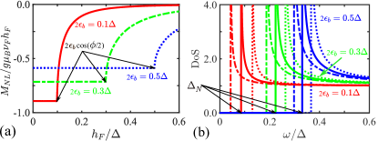
Fig. 4 (a) shows the field dependence of $M_{NL}$. The magnetization is given in units of $g\mu_{B}\nu_{F}h_{F}$, and hence the full spin screening corresponds to the value $-1$ in the curves. Here, different curves correspond to different choices of the barrier energies, $\epsilon_{b}$. The maximum effect occurs for $h^{max}_{F}=2\epsilon_{b}\cos(\phi/2)$. In the limit $\epsilon_{b}\ll\Delta$, $h^{max}_{F}\simeq\Delta_{N}$ (Eq. S51, red curves in Fig. 4). On the other hand, we find the weakening of spin screening with increasing the barrier energy, $\epsilon_{b}$ or minigap, $\Delta^{0}_{N}$. This can be understood from the spin resolved DoS in Fig. 4(b). Here, $N^{\uparrow}(\omega)$ and $N^{\downarrow}(\omega)$, are related to each other by a BCS-like DoS, $N_{BCS}(\omega,\Delta_{N})$ with a renormalized minigap, $\Delta_{N}$ (Eq. S53). Thus, $N^{\uparrow}(\omega)=N_{BCS}(\omega-\alpha_{r}h_{F},\Delta_{N})$ and $N^{\downarrow}(\omega)=N_{BCS}(\omega+\alpha_{r}h_{F},\Delta_{N})$, where $\alpha_{r}=(1-2\epsilon_{b}/\Delta)<1$ in the limit of $\epsilon_{b}\ll\Delta$ (Eq. S54). The full spin screening corresponds to $\alpha_{r}=1$ (Fig. 1b of main text). However, the failure of full screen is a result of the reduction of the spin-splitting due to the superconducting proximity effect. It becomes more obvious for larger $\Delta_{N}$ ($\epsilon_{b}$), (Eq. S54 and blue curves in Figs. 4).

Figure 4: (Color online.) Nonlocal magnetization, $M_{NL}$ of SC/NW-FI/SC structure. Panel (a) plots the field, $h_{F}$ dependence of $M_{NL}$, in the unit of $g\mu_{B}\nu_{F}h_{F}$, and hence the full spin screening means value of $-1$. The corresponding DoS are plotted in panel (b), where $h_{F}=0.05\Delta$. Other parameters: $T=0$, $\epsilon_{so}=0$ and $\phi=0$.

In the presence of the SR, we find a spin dependent renormalization of the frequency, see Eq. (S42). This implies a renormalization of the effective exchange field. For the sake of simplicity, let us consider the case of a small SR rate, $\epsilon_{so},\epsilon_{b}\ll\Delta_{N}$, and hence $\Delta^{0}_{N}\simeq 2\epsilon_{b}$. The first order correction to the normal Green function can be included by replacing the GFs, $G^{\eta}_{N}$ and $F^{\eta}_{N}$ on the right hand side of Eq. (S40), by the GFs, $\mathcal{G}^{\eta}_{N}$ and $\mathcal{F}^{\eta}_{N}$ in Eqs. (S46) and (S47). Then, we reach

$$G_{N}^{\eta} =\frac{-i(\omega^{\eta}_{r}+\eta h_{r}^{\eta})}{\sqrt{\left(\Delta^{\eta}_{r}\right)^{2}-\left(\omega^{\eta}_{r}+\eta h_{r}^{\eta}\right)^{2}}}.$$ (S55)

In the present limit, $\epsilon_{so}\ll\Delta_{N}$, the SR then leads to the following renormalization of frequency, minigap, and effective excahnge field:

$$\omega+i\Delta^{0}_{N}\mathcal{G}_{S}\rightarrow\omega^{\eta}_{r}\simeq(\omega+i\Delta^{0}_{N}\mathcal{G}_{S})\left(1+\frac{2\epsilon_{so}}{\Lambda(\eta h_{F})}\right),$$ (S56)

$$\Delta_{N}\mathcal{F}_{S}\rightarrow\Delta^{\eta}_{r}\simeq\Delta_{N}\mathcal{F}_{S}\left(1+\frac{2\epsilon_{so}}{{\Lambda(\eta h_{F})}}\right),$$ (S57)

$$h_{F}\rightarrow h^{\eta}_{r}\simeq h_{F}\left(1-\frac{2\epsilon_{so}}{\Lambda(\eta h_{F})}\right),$$ (S58)

with

$$\Lambda(\eta h_{F})=\sqrt{\left(\Delta_{N}\mathcal{F}_{S}\right)^{2}-\left(\omega+i\Delta^{0}_{N}\mathcal{G}_{S}-\eta h_{F}\right)^{2}}.$$ (S59)

Thus, the DoS of NW in the first order of SR reads

$$N^{\eta} \simeq\left|\mathrm{Re}\left\{\frac{|\omega^{\eta}_{r}+\eta h^{\eta}_{r}|}{\sqrt{|\omega^{\eta}_{r}+\eta h^{\eta}_{r}|^{2}-\left(\Delta^{\eta}_{r}\right)^{2}}}\right\}\right|,$$ (S60)

For spin block $\eta$, the coherent peaks in the spin-splitting DOS are given by

$$\omega^{\eta}_{\pm} =\pm\Delta_{N}\mathcal{F}_{S}(\omega^{\eta}_{\pm})-i\Delta^{0}_{N}\mathcal{G}_{S}(\omega^{\eta}_{\pm})$$ (S61)

$$-\eta h\left(\frac{\Lambda^{\pm}(\eta h_{F})-2\epsilon_{so}}{\Lambda^{\pm}(\eta h_{F})+2\epsilon_{so}}\right),$$

with

$$\Lambda^{\pm}(\eta h_{F})=\sqrt{\left(\Delta_{N}\mathcal{F}^{\eta}_{\pm}\right)^{2}-\left(\omega^{\eta}_{\pm}+i\Delta^{0}_{N}\mathcal{G}^{\eta}_{\pm}-\eta h_{F}\right)^{2}}.$$ (S62)

In the limit of $\Delta_{N}\ll\Delta$, we have $\mathcal{G}_{S}(\omega^{\eta}_{\pm})\simeq 0$ and $\mathcal{F}_{S}(\omega^{\eta}_{\pm})\simeq 1$. Hence, Eq. (S61) reduces into

$$\omega^{\eta}_{\pm}=\pm\Delta_{N}-\eta h\left(\frac{\Lambda^{\pm}(\eta h_{F})-2\epsilon_{so}}{\Lambda^{\pm}(\eta h_{F})+2\epsilon_{so}}\right).$$ (S63)

with

$$\Lambda^{\pm}(\eta h_{F})\simeq\sqrt{\left(\Delta_{N}\right)^{2}-\left(\omega^{\eta}_{\pm}-\eta h_{F}\right)^{2}}.$$ (S64)

For a small SR rate, $\epsilon_{so}\ll\Delta_{N}$, we can approximately replace the $\omega^{\eta}_{\pm}$ in the right hand side of Eq. (S63) by Eq. (S50). Thus, we arrive at

$$\omega^{\eta}_{\pm}\simeq\pm\Delta_{N}-\eta h_{F}\left(\frac{\sqrt{\pm\Delta_{N}\eta h_{F}-h^{2}_{F}}-\epsilon_{so}}{\sqrt{\pm\Delta_{N}\eta h_{F}-h^{2}_{F}}+\epsilon_{so}}\right).$$ (S65)

For zero temperature, we are only interested in the spin splitting of negative frequency

$$\omega^{+}_{-}\simeq-\Delta_{N}-h_{F}\left(\frac{i\sqrt{\Delta_{N}h_{F}+h^{2}_{F}}-\epsilon_{so}}{i\sqrt{\Delta_{N}h_{F}+h^{2}_{F}}+\epsilon_{so}}\right),$$ (S66)

$$\omega^{-}_{-}\simeq-\Delta_{N}+h_{F}\left(\frac{\sqrt{\Delta_{N}h_{F}-h^{2}_{F}}-\epsilon_{so}}{\sqrt{\Delta_{N}h_{F}-h^{2}_{F}}+\epsilon_{so}}\right).$$ (S67)

Thus the effective exchange field reads

$$h_{eff} =\frac{h_{F}}{2}\mathrm{Re}\left\{\frac{i\sqrt{\Delta_{N}h_{F}+h^{2}_{F}}-\epsilon_{so}}{i\sqrt{\Delta_{N}h_{F}+h^{2}_{F}}+\epsilon_{so}}\right.$$ (S68)

$$+\left.\frac{\sqrt{\Delta_{N}h_{F}-h^{2}_{F}}-\epsilon_{so}}{\sqrt{\Delta_{N}h_{F}-h^{2}_{F}}+\epsilon_{so}}\right\}.$$

For $h_{F}<\Delta_{N}$, we reach

$$\frac{h_{eff}}{h_{F}}\simeq 1-\frac{\epsilon^{2}_{so}}{\Delta_{N}h_{F}+h^{2}_{F}+\epsilon_{so}^{2}}-\frac{\epsilon_{so}}{\sqrt{\Delta_{N}h_{F}-h^{2}_{F}}+\epsilon_{so}}.$$ (S69)

For $h_{F}>\Delta_{N}$, we reach

$$\frac{h_{eff}}{h_{F}}=1-\frac{\epsilon^{2}_{so}}{\Delta_{N}h_{F}+h^{2}_{F}+\epsilon_{so}^{2}}-\frac{\epsilon^{2}_{so}}{h^{2}_{F}-\Delta_{N}h_{F}+\epsilon_{so}^{2}}.$$ (S70)

Clearly, we find that the effective exchange field decreases in the presence of the SR. This causes a shift to the right of the nonlocal magnetization curve as a function of the exchange field, see the blue dashed curve in Fig. 2(c) of the main text.

B.2 The SC-FI-SC NW structure

In this section we consider a more realistic setup, the lateral SC-FI-SC NW structure depicted in Fig. 3(a) of main text. Here, an arbitrary long normal wire (NW) is grown on the top of FI. Two superconductors (SCs) with phase difference, $\phi$ cover partially teh extremes of the NW. The starting point is agian the Usadel equation for the retarded quasiclassical Green’s function in the NW:

$$D\boldsymbol{\nabla}[\check{g}^{\eta}_{N}(\boldsymbol{r}) \boldsymbol{\nabla}\check{g}^{\eta}_{N}(\boldsymbol{r})]+i\left[\left(\omega+\eta h_{b}(\boldsymbol{r})\right)\hat{\tau}_{3},\check{g}^{\eta}_{N}(\boldsymbol{r})\right]=0,$$ (S71)

where we have neglected the SR. The magnetic proximity effect of FI can be described by a localized exchange field at FI/NW interface, $h_{b}(\boldsymbol{r})=bh_{ex}\theta_{F}(x)\delta(y)$, with

$$\theta_{F}(x)=\left\{\begin{matrix}1,&\frac{L_{N}}{2}-\frac{L_{F}}{2}<x<\frac{L_{N}}{2}+\frac{L_{F}}{2};\\ 0,&\textit{otherwise},\end{matrix}\right.$$ (S72)

where $L_{F}$ is the length of FI. On the other hand, the proximity effect of SCs is captured by the Kupriyanov-Lukichev boundary conditions (S2) at two NW/SC interfaces, which can be written in a compact form

$$\sigma_{N}[\check{g}_{N}(\boldsymbol{r}) \left.\partial_{y}\check{g}_{N}(\boldsymbol{r})]\right|_{y=W_{N}}=\frac{1}{R_{\square}}[\theta_{L}(x)+\theta_{R}(x)]$$

$$\times\left.\left[\check{g}_{N}(\boldsymbol{r}),\check{g}_{S}(\boldsymbol{r})\right]\right|_{y=W_{N}}.$$ (S73)

The positions of the left and right superconducting electrodes, in $x$ direction, are respectively described by two step-like functions

$$\theta_{L}(x)=\left\{\begin{matrix}1,&0<x<L_{S};\\ 0,&\textit{otherwise},\end{matrix}\right.$$ (S74)

$$\theta_{R}(x)=\left\{\begin{matrix}1,&L_{N}-L_{S}<x<L_{N};\\ 0,&\textit{otherwise},\end{matrix}\right.$$ (S75)

with $L_{S}$ being the length of both SCs. We do not consider the inverse proximity effect of FI on SCs and hence their GFs are the BCS ones

$$\left.\check{g}_{S}(\boldsymbol{r})\right|_{y=W_{N}} =\theta_{R}(x)\left\{\mathcal{G}_{S}\hat{\tau}_{3}+\mathcal{F}_{S}[\cos(\frac{\phi}{2})\hat{\tau}_{1}-\sin(\frac{\phi}{2})\hat{\tau}_{2}]\right\}$$

$$+\theta_{L}(x)\left\{\mathcal{G}_{S}\hat{\tau}_{3}+\mathcal{F}_{S}[\cos(\frac{\phi}{2})\hat{\tau}_{1}+\sin(\frac{\phi}{2})\hat{\tau}_{2}]\right\},$$ (S76)

where we introduce phase difference, $\phi$ between SCs.

Because the transverse dimensions of the NW are smaller than the characteristic length $\xi_{N}$, we can assume that the GFs do not depend on $y$ and $z$. We can then integrate the Usadel equation, (S71), first over $z$-direction, where the zero current BC at both vacuum/NW interfaces applies, Eq. (S3), and second over the $y$-direction. In the second integration the local exchange field at the NW/FI at $y=0$ results in an effective spin-splitting field $h_{F}$, whereas at the SC/NW interface, ,$y=W_{N}$, the boundary condition, Eq. (B.2) introduces a term in the Usadel equation describing the induced superconducting condensate. The final 1D equation after these integrations reads:

$$D\partial_{x} [\check{g}^{\eta}_{N}(x)\partial_{x}\check{g}^{\eta}_{N}(x)]+i\left[\left(\omega+\theta_{F}(x)\eta h_{F}\right)\hat{\tau}_{3},\check{g}^{\eta}_{N}(x)\right]$$

$$=\left.\epsilon_{b}[\theta_{L}(x)+\theta_{R}(x)]\left[\check{g}_{S}(\boldsymbol{r}),\check{g}^{\eta}_{N}(x)\right]\right|_{y=W_{N}}.$$ (S77)

The strength of the superconducting proximity effect is parametrized by the energy:

$$\epsilon_{b}=D/(W_{N}\sigma_{N}R_{\square}).$$ (S78)

Eq. (B.2) is complemented by the normalization condition, $\check{g}^{2}_{N}(x)=1$. In order to solve numerically these two matrix equations it is convenient to use the Riccati parameterization to express the GFs in terms of two coherent functions $\gamma$ and $\tilde{\gamma}$ as follows:

$$\check{g}=\check{N}\begin{bmatrix}1-\gamma\tilde{\gamma}&2\gamma\\ 2\tilde{\gamma}&\tilde{\gamma}\gamma-1\end{bmatrix}=\begin{bmatrix}\mathcal{G}&\mathcal{F}\\ \tilde{\mathcal{F}}&\tilde{\mathcal{G}}\end{bmatrix},$$ (S79)

with

$$\check{N}=\begin{bmatrix}(1+\gamma\tilde{\gamma})^{-1}&0\\ 0&(1+\tilde{\gamma}\gamma)^{-1}\end{bmatrix}.$$ (S80)

where $\mathcal{F}$ and $\tilde{\mathcal{F}}$ describe the Cooper pairs penetrating from both S regions. In Riccati parameterization, Usadel equation (B.2), for each spin block $\eta=\pm$, reads

$$\gamma^{\prime\prime}_{\eta} =\gamma^{\prime}_{\eta}\tilde{\mathcal{F}}_{\eta}\gamma^{\prime}_{\eta}-2i[\omega_{r}(l)+\eta h_{F}\theta_{F}(l)]\gamma_{\eta}$$ (S81)

$$-\alpha_{N}\mathcal{F}_{S}(l)+\alpha_{N}\tilde{\mathcal{F}}_{S}(l)\gamma^{2}_{\eta},$$

$$\tilde{\gamma}^{\prime\prime}_{\eta} =\tilde{\gamma}^{\prime}_{\eta}\mathcal{F}_{\eta}\tilde{\gamma}^{\prime}_{\eta}-2i[\omega_{r}(l)+\eta h_{F}\theta_{F}(l)]\gamma_{\eta}$$ (S82)

$$-\alpha_{N}\tilde{\mathcal{F}}_{S}(l)+\alpha_{N}\mathcal{F}_{S}(l)\tilde{\gamma}^{2}_{\eta},$$

with

$$\omega^{\eta}_{r}(l)=\omega+i\alpha_{N}\mathcal{G}_{S}[\theta_{L}(l)+\theta_{R}(l)],$$ (S83)

$$\mathcal{F}_{S}(l)=\mathcal{F}_{S}[\theta_{L}(l)e^{-i\phi/2}+\theta_{R}(l)e^{+i\phi/2}],$$ (S84)

$$\tilde{\mathcal{F}_{S}}(l)=\mathcal{F}_{S}[\theta_{L}(l)e^{+i\phi/2}+\theta_{R}(l)e^{-i\phi/2}],$$ (S85)

where $\alpha_{N}=L_{N}^{2}/(W_{N}\sigma_{N}R_{\square})$, and we have made the position coordinate dimensionless by introducing $l=x/L_{N}$ and energy is in the unit of $\epsilon_{th}=D/L_{N}^{2}$.

Figure 5: (Color online.) Nonlocal magnetization, $M_{NL}$ of SC-FI-SC NW structure. Panels (a,b) plot the $M_{NL}$ of as a function of (a) $h_{F}/\Delta$ and (c) $\phi$, respectively, where $X=0$, $\epsilon_{b}=0.05\Delta$ and $L=\xi_{0}/3$. Panel (c) shows $M_{NL}$ as a function of $h_{F}/\Delta$ and $X/L_{N}$, where $\phi=0$, $\epsilon_{b}=0.5\Delta$ and $L=4.7\xi_{0}$. While panel (d) shows the corresponding local DoS, $N(\omega,X)$. The red curve represents the pseudogap, $\Delta_{N}^{*}(X)$. Other parameters: $T=0$, $\epsilon_{so}=0$, $\epsilon_{b}=0.5\Delta$, $\phi=0$, $\xi_{0}=\sqrt{D/\Delta}$, $L_{F}=L_{N}$ and $L_{S}=L_{N}/3$.

In a more realistic setup, the length of the NW, $L_{N}$ can be larger than the characteristic length $\xi_{N}$. Moreover, the NW can be partially covered by the SCs films of length, $L_{S}$. We assume that the NW is grown on top of a FI substrate with length, $L_{F}$. Hereafter, we assume a symmetric setup with $L_{S}=L_{N}/3$, and hence the distance between the SC leads is $L=L_{N}/3$. The minigap induced in the NW, $\Delta_{N}$ depends on this distance and the NW/SC barrier resistance.

Let us begin with the case of weak superconducting proximity, $\epsilon_{b}=0.05\Delta$ and short NW, $L=\xi_{0}/3$, where $\xi_{0}=\sqrt{D/\Delta}$. Fig. 5(a) shows the $h_{F}$ dependence of $M_{NL}$ at the center of NW for different values of the phase difference, $\phi$. As far as $h_{F}<\Delta_{N}$, $M_{NL}W_{N}A$ compensates the Pauli magnetic moment $\int_{b}M_{\textrm{Pauli}}=g\mu_{B}\nu_{F}h_{ex}bA$ localized at the FI/NM interface, with $A$ being the area of FI/NW interface. At $h_{F}=\Delta_{N}$, $M_{NL}$ reaches a maximum value, $g\mu_{B}\nu_{F}\Delta_{N}$ and decays as $h_{F}-\sqrt{h_{F}^{2}-\Delta_{N}^{2}}$ for $h_{F}>\Delta_{N}$ Bergeret et al. (2005); Karchev et al. (2001); Shen et al. (2003). In Fig. 4(b), we show the phase difference, $\phi$ dependence of $M_{NL}$ at the center of NW for different values of $h_{F}$. The maximum minigap is about $\Delta_{N}^{0}\simeq 0.032\Delta$. When $h_{F}\leq\Delta_{N}^{0}$, $M_{NL}$ remains constant for all phases smaller than $\arccos{h_{F}/\Delta_{N}^{0}}$ (red curve in Fig. 4b). In other words, as far as $h_{F}$ is smaller than the induced gap $\Delta_{N}=\Delta_{N}^{0}\cos(\phi/2)$, the $M_{NL}(\phi)$ curve shows a plateau at the value opposite to $M_{\textrm{Pauli}}$. The maximum modulation is achieved for $h_{F}=\Delta^{0}_{N}$ (green curve in Fig. 4 b). For larger values of $h_{F}$, $M_{NL}$ the NW is gapless and $M_{NL}(\phi)$ is overall reduced (blue curve).

Figure 6: (Color online.) Nonlocal magnetization of the long NW partially covered by FI. Panels (a,b) show $M_{NL}$ as a function of (a) $X/L$ and (b) $\phi$. We set $\phi=0$ in panel (a) and $X=0$ in panel (b). Other parameters: $T=0$, $\epsilon_{so}=0$, $\epsilon_{b}=0.5\Delta$, $\xi_{0}=\sqrt{D/\Delta}$, $L=2.4\xi_{0}$, $L_{F}=L_{N}/4$ and $L_{S}=L_{N}/3$.

Let us now go beyond the limits of weak superconducting proximity and short NW. The results are plotted in Fig. 5 , where $\epsilon_{b}=0.5\Delta$ and $L=4.7\xi_{0}$. In this case, the local DoS, $N(\omega,X)$ strongly depends on $X$ (Fig. 5d here and Fig. 3b of main text). The induced minigap, $\Delta_{N}$, though is spatially constant, as shown by the green line in Fig. 5(d). The local pseudogap, $\Delta_{N}^{*}(X)$ defined by the energy in which the exact DoS, $N(\omega,X)$ coincide with the DOS in the normal state, $N_{0}(\omega,X)=1$, is position-dependent, as shown by the red curves in Fig. 5(d). It is smallest at the center, $\Delta^{*}_{N}(0)\simeq\Delta_{N}$, and becomes bigger closer to both ends. At zero temperature, the calculation of the local $M_{NL}(X)$, Eq. (1) of the main text, can be well approximated by replacing the exact DoS, $N(\omega,X)$ by a BCS-like one, $N_{BCS}(\omega,\Delta^{*}_{N}(X))$ with the position-dependent gap, $\Delta^{*}_{N}(X)$.

Panel 5(c) depicts $M_{NL}$ as a function of $h_{F}/\Delta$ and $X/L_{N}$. We find a interesting transition from a maximum to a minimum at $X=0$ in the $M_{NL}(X)$ dependence. For small $h_{F}$, the shape with a minimum is due to the weakening of spin screening with increasing pseudo gap, $\Delta_{N}^{*}(X)$ from center to both ends.

In Fig. 6 we show the nonlocal magnetization in a setup when the FI is in contact only to certain portion of the NW, for example if $L_{F}/L_{N}=1/4$. In Fig. 6 (a), we show the spatial dependence of $M_{NL}$ for different values of $h_{F}$ and in panel (b) the phase-dependence at $x=0$.

References

Lutchyn et al. (2010)R. M. Lutchyn, J. D. Sau, and S. D. Sarma, Physical review
letters 105, 077001
(2010).
Oreg et al. (2010)Y. Oreg, G. Refael, and F. von Oppen, Physical review letters 105, 177002 (2010).
Mourik et al. (2012)V. Mourik, K. Zuo,
S. M. Frolov, S. Plissard, E. P. Bakkers, and L. P. Kouwenhoven, Science 336, 1003 (2012).
Rokhinson et al. (2012)L. P. Rokhinson, X. Liu, and J. K. Furdyna, Nature Physics 8, 795 (2012).
Das et al. (2012)A. Das, Y. Ronen, Y. Most, Y. Oreg, M. Heiblum, and H. Shtrikman, Nature Physics 8, 887 (2012).
Finck et al. (2013)A. Finck, D. J. Van Harlingen, P. Mohseni, K. Jung, and X. Li, Physical review letters 110, 126406 (2013).
Albrecht et al. (2016)S. M. Albrecht, A. P. Higginbotham, M. Madsen, F. Kuemmeth,
T. S. Jespersen, J. Nygård, P. Krogstrup, and C. Marcus, Nature 531, 206 (2016).
Deng et al. (2016)M. Deng, S. Vaitiekėnas, E. B. Hansen, J. Danon,
M. Leijnse, K. Flensberg, J. Nygård, P. Krogstrup, and C. M. Marcus, Science 354, 1557 (2016).
Suominen et al. (2017)H. J. Suominen, M. Kjaergaard, A. R. Hamilton, J. Shabani,
C. J. Palmstrøm,
C. M. Marcus, and F. Nichele, Physical review letters 119, 176805 (2017).
Nichele et al. (2017)F. Nichele, A. C. Drachmann, A. M. Whiticar, E. C. O?Farrell, H. J. Suominen, A. Fornieri,
T. Wang, G. C. Gardner, C. Thomas, A. T. Hatke, et al., Physical review letters 119, 136803 (2017).
Takei et al. (2013)S. Takei, B. M. Fregoso,
H.-Y. Hui, A. M. Lobos, and S. D. Sarma, Physical review letters 110, 186803 (2013).
Chang et al. (2015)W. Chang, S. Albrecht,
T. Jespersen, F. Kuemmeth, P. Krogstrup, J. Nygård, and C. M. Marcus, Nature nanotechnology 10, 232 (2015).
Lutchyn et al. (2011)R. M. Lutchyn, T. D. Stanescu, and S. D. Sarma, Physical review letters 106, 127001 (2011).
Qi and Zhang (2011)X.-L. Qi and S.-C. Zhang, Reviews of Modern
Physics 83, 1057
(2011).
Elliott and Franz (2015)S. R. Elliott and M. Franz, Reviews
of Modern Physics 87, 137 (2015).
Alicea (2012)J. Alicea, Reports on progress in physics 75, 076501 (2012).
Lutchyn et al. (2018)R. t. Lutchyn, E. Bakkers,
L. P. Kouwenhoven,
P. Krogstrup, C. Marcus, and Y. Oreg, Nature Reviews Materials 3, 52 (2018).
Sarma et al. (2015)S. D. Sarma, M. Freedman, and C. Nayak, npj Quantum
Information 1, 15001
(2015).
Stanescu and Tewari (2013)T. D. Stanescu and S. Tewari, Journal of Physics: Condensed Matter 25, 233201 (2013).
Bergeret et al. (2018)F. S. Bergeret, M. Silaev,
P. Virtanen, and T. T. Heikkilä, Reviews of Modern
Physics 90, 041001
(2018).
Giazotto and Taddei (2008)F. Giazotto and F. Taddei, Physical Review B 77, 132501 (2008).
Yang et al. (2013)H.-X. Yang, A. Hallal,
D. Terrade, X. Waintal, S. Roche, and M. Chshiev, Physical review letters 110, 046603 (2013).
Eremeev et al. (2013)S. Eremeev, V. Men’Shov,
V. Tugushev, P. M. Echenique, and E. V. Chulkov, Physical Review B 88, 144430 (2013).
Virtanen et al. (2018)P. Virtanen, F. Bergeret,
E. Strambini, F. Giazotto, and A. Braggio, Physical Review B 98, 020501 (2018).
Wei et al. (2016)P. Wei, S. Lee, F. Lemaitre, L. Pinel, D. Cutaia, W. Cha, F. Katmis, Y. Zhu,
D. Heiman, J. Hone, et al., Nature materials 15, 711 (2016).
Katmis et al. (2016)F. Katmis, V. Lauter,
F. S. Nogueira, B. A. Assaf, M. E. Jamer, P. Wei, B. Satpati, J. W. Freeland, I. Eremin, D. Heiman,
et al., Nature 533, 513
(2016).
Hao et al. (1991)X. Hao, J. Moodera, and R. Meservey, Physical review letters 67, 1342 (1991).
Meservey et al. (1970)R. Meservey, P. Tedrow, and P. Fulde, Physical Review
Letters 25, 1270
(1970).
Hao et al. (1990)X. Hao, J. Moodera, and R. Meservey, Physical Review B 42, 8235 (1990).
Strambini et al. (2017)E. Strambini, V. Golovach,
G. De Simoni, J. Moodera, F. Bergeret, and F. Giazotto, Phys. Rev. Mater. 1, 054402 (2017).
Moodera et al. (1988)J. Moodera, X. Hao,
G. Gibson, and R. Meservey, Physical review letters 61, 637 (1988).
Rouco et al. (2019)M. Rouco, S. Chakraborty,
F. Aikebaier, V. N. Golovach, E. Strambini, J. S. Moodera, F. Giazotto, T. T. Heikkilä, and F. S. Bergeret, Physical Review B 100, 184501 (2019).
Liu et al. (2019)Y. Liu, S. Vaitiekenas,
S. Martí-Sánchez,
C. Koch, S. Hart, Z. Cui, T. Kanne, S. A. Khan,
R. Tanta, S. Upadhyay, et al., Nano letters 20, 456 (2019).
Sau et al. (2010)J. D. Sau, R. M. Lutchyn,
S. Tewari, and S. D. Sarma, Physical review letters 104, 040502 (2010).
Lee et al. (2012)S.-P. Lee, J. Alicea, and G. Refael, Physical review letters 109, 126403 (2012).
Livanas et al. (2019)G. Livanas, M. Sigrist, and G. Varelogiannis, Scientific
reports 9, 1 (2019).
Abrikosov and Gor?kov (1962)A. A. Abrikosov and L. P. Gor?kov, J.
Exp. Theor. Phys. 15, 752 (1962).
Larkin and Varlamov (2005)A. Larkin and A. Varlamov, Theory of fluctuations
in superconductors (Clarendon Press, 2005).
Fulde and Ferrell (1964)P. Fulde and R. A. Ferrell, Physical Review 135, A550 (1964).
Bergeret et al. (2005)F. Bergeret, A. F. Volkov, and K. B. Efetov, Reviews of modern physics 77, 1321 (2005).
Karchev et al. (2001)N. Karchev, K. Blagoev,
K. Bedell, and P. Littlewood, Physical review letters 86, 846 (2001).
Shen et al. (2003)R. Shen, Z. Zheng,
S. Liu, and D. Xing, Physical Review B 67, 024514 (2003).
Note (1)Strictly speaking, for a large enough field , the
superconducting gap has to be determined self-consistently, and a
inhomogeneoues superconducting phase may appear Larkin and Varlamov (2005); Fulde and Ferrell (1964). The situation is simpler when
superconductivity is induced in a non-superconducting material via the
proximity effect. In this case the self-consistency is not needed and the
exchange field can be arbitrary large. This is the case considered in the
rest of the manuscript.
Zhang et al. (2019)X.-P. Zhang, F. S. Bergeret,
and V. N. Golovach, Nano letters 19, 6330 (2019).
Bergeret et al. (2000)F. Bergeret, K. Efetov, and A. Larkin, Physical Review
B 62, 11872 (2000).
Bergeret et al. (2004a)F. Bergeret, A. Volkov, and K. Efetov, Physical Review
B 69, 174504 (2004a).
Bergeret et al. (2004b)F. Bergeret, A. Volkov, and K. Efetov, EPL (Europhysics
Letters) 66, 111
(2004b).
Dahir et al. (2019)S. M. Dahir, A. F. Volkov, and I. M. Eremin, Physical Review
B 100, 134513 (2019).
Xia et al. (2009)J. Xia, V. Shelukhin,
M. Karpovski, A. Kapitulnik, and A. Palevski, Physical review letters 102, 087004 (2009).
Salikhov et al. (2009a)R. Salikhov, I. Garifullin, N. Garif?yanov, L. Tagirov, K. Theis-Bröhl, K. Westerholt, and H. Zabel, Physical review letters 102, 087003 (2009a).
Salikhov et al. (2009b)R. Salikhov, N. Garif?yanov, I. Garifullin, L. Tagirov,
K. Westerholt, and H. Zabel, Physical Review B 80, 214523 (2009b).
Usadel (1970)K. D. Usadel, Physical Review Letters 25, 507 (1970).
Giazotto et al. (2011)F. Giazotto, P. Spathis,
S. Roddaro, S. Biswas, F. Taddei, M. Governale, and L. Sorba, Nature Physics 7, 857 (2011).
Tiira et al. (2017)J. Tiira, E. Strambini,
M. Amado, S. Roddaro, P. San-Jose, R. Aguado, F. Bergeret, D. Ercolani, L. Sorba, and F. Giazotto, Nature communications 8, 1 (2017).
Iorio et al. (2018)A. Iorio, M. Rocci,
L. Bours, M. Carrega, V. Zannier, L. Sorba, S. Roddaro, F. Giazotto, and E. Strambini, Nano letters 19, 652 (2018).
Strambini et al. (2020)E. Strambini, A. Iorio,
O. Durante, R. Citro, C. Sanz-Fernández, C. Guarcello, I. Tokatly, A. Braggio, M. Rocci, N. Ligato, et al., arXiv preprint arXiv:2001.03393 (2020).
Kuprianov and Lukichev (1988)M. Y. Kuprianov and V. F. Lukichev, J.
Exp. Theor. Phys. 67, 1163 (1988).
(60)See supplementary materials for the
derivation of Usadel equations which includes Refs.
Hammer et al. (2007); Kuprianov and Lukichev (1988); Abrikosov and Gor?kov (1962); Larkin and Varlamov (2005); Fulde and Ferrell (1964); Zhang et al. (2019); Bergeret et al. (2000, 2005); Karchev et al. (2001); Shen et al. (2003) .
Seviour and Volkov (2000) R. Seviour and A. Volkov, Physical Review B 61, R9273 (2000).
Börlin et al. (2002)J. Börlin, W. Belzig,
and C. Bruder, Physical review
letters 88, 197001
(2002).
Bezuglyi et al. (2011)E. Bezuglyi, E. Bratus, and V. Shumeiko, Physical Review
B 83, 184517 (2011).
(64)In fact, in the limit , the effective exchange field acting on the conducting
electrons becomes for and for
SM .
Villamor et al. (2013) E. Villamor, M. Isasa, L. E. Hueso, and F. Casanova, Physical Review B 87, 094417 (2013).
Murzyn et al. (2003)P. Murzyn, C. Pidgeon,
P. Phillips, M. Merrick, K. Litvinenko, J. Allam, B. Murdin, T. Ashley, J. Jefferson, A. Miller, et al., Applied Physics Letters 83, 5220 (2003).
Song and Kim (2002)P. H. Song and K. Kim, Physical Review
B 66, 035207 (2002).
Murdin et al. (2005)B. Murdin, K. Litvinenko,
J. Allam, C. Pidgeon, M. Bird, K. Morrison, T. Zhang, S. Clowes, W. Branford, J. Harris, et al., Physical Review B 72, 085346 (2005).
Kjærgaard et al. (2016)M. Kjærgaard, F. Nichele, H. J. Suominen, M. Nowak,
M. Wimmer, A. Akhmerov, J. Folk, K. Flensberg, J. Shabani, w. C. Palmstrøm, et al., Nature communications 7, 1 (2016).
Le Sueur et al. (2008)H. Le Sueur, P. Joyez,
H. Pothier, C. Urbina, and D. Esteve, Physical review letters 100, 197002 (2008).
Giazotto et al. (2010)F. Giazotto, J. T. Peltonen, M. Meschke, and J. P. Pekola, Nature Physics 6, 254 (2010).
Meschke et al. (2011)M. Meschke, J. Peltonen,
J. P. Pekola, and F. Giazotto, Physical Review B 84, 214514 (2011).
Giazotto and Taddei (2011)F. Giazotto and F. Taddei, Physical Review B 84, 214502 (2011).
Ronzani et al. (2014)A. Ronzani, C. Altimiras,
and F. Giazotto, Physical Review
Applied 2, 024005
(2014).
Strambini et al. (2016)E. Strambini, S. D’Ambrosio, F. Vischi,
F. Bergeret, Y. V. Nazarov, and F. Giazotto, Nature Nanotechnology 11, 1055 (2016).
Ronzani et al. (2017)A. Ronzani, S. D’Ambrosio,
P. Virtanen, F. Giazotto, and C. Altimiras, Physical Review B 96, 214517 (2017).
Fornieri et al. (2019)A. Fornieri, A. M. Whiticar, F. Setiawan,
E. Portolés, A. C. Drachmann, A. Keselman, S. Gronin, C. Thomas, T. Wang, R. Kallaher, et al., Nature 569, 89 (2019).
Xiong et al. (2011)Y. Xiong, S. Stadler,
P. Adams, and G. Catelani, Physical review letters 106, 247001 (2011).
Hammer et al. (2007)J. Hammer, J. C. Cuevas,
F. Bergeret, and W. Belzig, Physical Review B 76, 064514 (2007).