EUROPEAN ORGANIZATION FOR NUCLEAR RESEARCH (CERN)

​​​ CERN-EP-2020-008 LHCb-PAPER-2019-030 12 August 2020

Measurement of the branching fraction of the decay ${{B}^{0}_{s}}\!\rightarrow{{K}^{0}_{\mathrm{S}}}{{K}^{0}_{\mathrm{S}}}$

LHCb collaboration

A measurement of the branching fraction of the decay ${{B}^{0}_{s}}\!\rightarrow{{K}^{0}_{\mathrm{S}}}{{K}^{0}_{\mathrm{S}}}$ is performed using proton–proton collision data corresponding to an integrated luminosity of $5\text{\,}\text{\,fb}^{-1}$ collected by the LHCb experiment between 2011 and 2016. The branching fraction is determined to be

$${\mathcal{B}}(\mbox{${{B}^{0}_{s}}\!\rightarrow{{K}^{0}_{\mathrm{S}}}{{K}^{0}_{\mathrm{S}}}$})=[8.3\pm 1.6\,(\text{stat})\pm 0.9\,(\text{syst})\pm 0.8\,(\text{norm})\pm 0.3\,(\nicefrac{{f_{s}}}{{f_{d}}})]\times 10^{-6}\,,$$

where the first uncertainty is statistical, the second is systematic, and the third and fourth are due to uncertainties on the branching fraction of the normalization mode ${{B}^{0}}\!\rightarrow\phi{{K}^{0}_{\mathrm{S}}}$ and the ratio of hadronization fractions $\nicefrac{{f_{s}}}{{f_{d}}}$. This is the most precise measurement of this branching fraction to date. Furthermore, a measurement of the branching fraction of the decay ${{B}^{0}}\!\rightarrow{{K}^{0}_{\mathrm{S}}}{{K}^{0}_{\mathrm{S}}}$ is performed relative to that of the ${{B}^{0}_{s}}\!\rightarrow{{K}^{0}_{\mathrm{S}}}{{K}^{0}_{\mathrm{S}}}$ channel, and is found to be

$$\frac{{\mathcal{B}}(\mbox{${{B}^{0}}\!\rightarrow{{K}^{0}_{\mathrm{S}}}{{K}^{0}_{\mathrm{S}}}$})}{{\mathcal{B}}(\mbox{${{B}^{0}_{s}}\!\rightarrow{{K}^{0}_{\mathrm{S}}}{{K}^{0}_{\mathrm{S}}}$})}=[7.5\pm 3.1\,(\text{stat})\pm 0.5\,(\text{syst})\pm 0.3\,(\nicefrac{{f_{s}}}{{f_{d}}})]\times 10^{-2}\,.$$

Published in Phys. Rev. D 102 (2020) 012011

© 2024 CERN for the benefit of the LHCb collaboration. CC-BY-4.0 licence.

 

1 Introduction

Flavour-changing neutral current processes, especially neutral $B$ meson decays to kaons and excited kaons, can be used as probes of the Standard Model and of the CKM unitarity triangle angle $\beta_{(s)}$. While decays such as $B^{0}_{(s)}\!\rightarrow{{K}^{*0}}{{\kern 1.99997pt\overline{\kern-1.99997ptK}{}}{}^{*0}}$, $B^{0}_{s}\!\rightarrow{{K}^{*0}}{{\kern 1.99997pt\overline{\kern-1.99997ptK}{}}{}^{0}}$, and ${{B}^{0}}\!\rightarrow{{K}^{+}}{{K}^{-}}$ have already been measured at the LHC [1, 2, 3, 4], decays of $b$ hadrons to final states containing only long-lived particles, such as ${K}^{0}_{\mathrm{S}}$ mesons or $\mathchar 28931\relax$ baryons, have never before been reported in a hadronic production environment. A measurement of the branching fraction of ${{B}^{0}_{s}}\!\rightarrow{{K}^{0}}{{\kern 1.99997pt\overline{\kern-1.99997ptK}{}}{}^{0}}$ decays can be used as input to future SM predictions, and is a first step toward a time-dependent measurement of $C\!P$ violation in this channel using future LHC data.

In the Standard Model, the decay amplitude of ${{B}^{0}_{s}}\!\rightarrow{{K}^{0}}{{\kern 1.99997pt\overline{\kern-1.99997ptK}{}}{}^{0}}$ is dominated by ${b}\rightarrow{s}{\overline{d}}{d}$ loop transitions with gluon radiation, while other contributions, including color singlet exchange, are suppressed to the level of $5\text{\,}\mathrm{\char 37\relax}$ [5] in the decay amplitude. Predictions of this branching fraction within the SM lie in the range $(15-25)\times 10^{-6}$ [6, 7, 8, 9], with calculations relying on a variety of theoretical approaches such as soft collinear effective theory, QCD factorisation, and perturbative leading-order and next-to-leading-order QCD. Beyond the Standard Model, possible contributions from new particles or couplings [10, 11, 5, 12, 13] can be probed by improved experimental precision on the branching fraction measurement.

The decay ${{B}^{0}_{s}}\!\rightarrow{{K}^{0}}{{\kern 1.99997pt\overline{\kern-1.99997ptK}{}}{}^{0}}$ was first observed by the Belle collaboration in 2016 [14]. The branching fraction was determined to be ${\mathcal{B}}(\mbox{${{B}^{0}_{s}}\!\rightarrow{{K}^{0}}{{\kern 1.99997pt\overline{\kern-1.99997ptK}{}}{}^{0}}$})=(19.6^{+5.8}_{-5.1}\pm 1.0\pm 2.0)\times 10^{-6}$, where the first uncertainty is statistical, the second systematic and the third due to the uncertainty of the total number of produced ${B}^{0}_{s}$–${\kern 1.79993pt\overline{\kern-1.79993ptB}{}}{}^{0}_{s}$ pairs. The related decay ${{B}^{0}}\!\rightarrow{{K}^{0}}{{\kern 1.99997pt\overline{\kern-1.99997ptK}{}}{}^{0}}$ has a branching fraction of $(1.21\pm 0.16)\times 10^{-6}$[15, 16, 17] in the world average.

This paper presents measurements of the branching fraction of ${{B}^{0}_{({s})}}\!\rightarrow{{K}^{0}_{\mathrm{S}}}{{K}^{0}_{\mathrm{S}}}$ decays using proton-proton collision data collected by the LHCb experiment at centre-of-mass energies $\sqrt{s}=7$, $8$, or $13\text{\,}\mathrm{T}\mathrm{e}\mathrm{V}$. The ${{B}^{0}_{({s})}}\!\rightarrow{{K}^{0}_{\mathrm{S}}}{{K}^{0}_{\mathrm{S}}}$ branching fraction is assumed to be half of the ${{B}^{0}_{({s})}}\!\rightarrow{{K}^{0}}{{\kern 1.99997pt\overline{\kern-1.99997ptK}{}}{}^{0}}$ branching fraction, as the ${K}^{0}$ ${\kern 1.99997pt\overline{\kern-1.99997ptK}{}}{}^{0}$ final state is $C\!P$ even. These ${B}^{0}_{({s})}$ branching fractions are determined relative to the ${{B}^{0}}\!\rightarrow\phi{{K}^{0}_{\mathrm{S}}}$ branching fraction, where the notation $\phi$ is used for the $\phi(1020)$ meson throughout. This normalization mode has a corresponding branching fraction equal to half of ${\mathcal{B}}(\mbox{${{B}^{0}}\!\rightarrow\phi{{K}^{0}}$})=$(7.3\pm\pm 0.7)\text{\times}{10}^{-6}$$ [18, 19], and is chosen for its similarity to the signal mode. Despite the smaller branching fraction, the yield of the normalization mode is much larger than that of the signal mode, because the near-instantaneous $\phi$ decay can be reconstructed more efficiently than a long-lived ${K}^{0}_{\mathrm{S}}$, and because for LHCb the production fraction of ${B}^{0}$ mesons is approximately four times that of ${B}^{0}_{s}$ mesons. [44, 45]. Throughout this paper, the decays ${{B}^{0}_{({s})}}\!\rightarrow{{K}^{0}_{\mathrm{S}}}{{K}^{0}_{\mathrm{S}}}$ and ${{B}^{0}}\!\rightarrow\phi{{K}^{0}_{\mathrm{S}}}$ are reconstructed using the decays ${{K}^{0}_{\mathrm{S}}}\!\rightarrow{{\pi}^{+}}{{\pi}^{-}}$ and $\phi\!\rightarrow{{K}^{+}}{{K}^{-}}$.

The paper is structured as follows. A brief description of the LHCb detector as well as the simulation and reconstruction software is given in Sec. 2. Signal selection and strategies to suppress background contributions are outlined in Sec. 3. The models to describe the invariant-mass components, the fitting and the normalization procedure are introduced in Sec. 4. Systematic uncertainties are discussed in Sec. 5. Finally, the results are summarized in Sec. 6.

2 LHCb detector

The LHCb detector [20, 21] is a single-arm forward spectrometer covering the pseudorapidity range $2<\eta<5$, designed for the study of particles containing $b$ or $c$ quarks. The detector includes a high-precision tracking system consisting of a silicon-strip vertex detector (VELO) surrounding the $pp$ interaction region [22], a large-area silicon-strip detector located upstream of a dipole magnet with a bending power of about $4{\mathrm{\,Tm}}$, and three stations of silicon-strip detectors and straw drift tubes [23, 24] placed downstream of the magnet. The tracking system provides a measurement of momentum, $p$, of charged particles with a relative uncertainty that varies from 0.5% at low momentum to 1.0% at 200$\text{\,Ge\kern-1.00006ptV\!/}c$. The minimum distance of a track to a primary vertex (PV), the impact parameter (IP), is measured with a resolution of $(15+29/p_{\mathrm{T}})\,\upmu\text{m}$, where $p_{\mathrm{T}}$ is the component of the momentum transverse to the beam, in $\text{\,Ge\kern-1.00006ptV\!/}c$. Different types of charged hadrons are distinguished using information from two ring-imaging Cherenkov detectors [25]. Photons, electrons and hadrons are identified by a calorimeter system consisting of scintillating-pad and preshower detectors, an electromagnetic calorimeter and a hadronic calorimeter. Muons are identified by a system composed of alternating layers of iron and multiwire proportional chambers.

The online event selection is performed by a trigger [26], which consists of a hardware stage, based on information from the calorimeter and muon systems, followed by a software stage, which applies a full event reconstruction. At the hardware trigger stage, events are required to contain a muon with high $p_{\mathrm{T}}$ or a hadron, photon or electron with high transverse energy in the calorimeters. In the software trigger, events are selected by a topological $b$-hadron trigger. At least one charged particle must have a large transverse momentum and be inconsistent with originating from any PV. A two- or three-track secondary vertex is constructed, which must have a large sum of the $p_{\mathrm{T}}$ of the charged particles and a significant displacement from any PV. A multivariate algorithm [27] is used for the identification of secondary vertices consistent with the decay of a $b$-hadron. This is used to collect both ${{B}^{0}_{({s})}}\!\rightarrow{{K}^{0}_{\mathrm{S}}}{{K}^{0}_{\mathrm{S}}}$ and ${{B}^{0}}\!\rightarrow\phi{{K}^{0}_{\mathrm{S}}}$ decays. In addition to this topological trigger and algorithm, some ${{B}^{0}}\!\rightarrow\phi{{K}^{0}_{\mathrm{S}}}$ decays are also collected using dedicated $\phi$ trigger requirements that exploit the topology of the $\phi\!\rightarrow{{K}^{+}}{{K}^{-}}$ decay and apply additional particle identification requirements to the charged kaons.

Simulation is required to model the effects of the detector acceptance and the imposed selection requirements. In simulation, $pp$ collisions are generated using Pythia [28, *Sjostrand:2007gs] with a specific LHCb configuration [30]. Decays of hadronic particles are described by EvtGen [31], in which final-state radiation is generated using Photos [32]. The interaction of the generated particles with the detector, and its response, are implemented using the Geant4 toolkit [33, *Agostinelli:2002hh] as described in Ref. [35].

3 Event selection

The decays ${{B}^{0}_{({s})}}\!\rightarrow{{K}^{0}_{\mathrm{S}}}{{K}^{0}_{\mathrm{S}}}$ and ${{B}^{0}}\!\rightarrow\phi{{K}^{0}_{\mathrm{S}}}$ are reconstructed using the decay modes ${{K}^{0}_{\mathrm{S}}}\!\rightarrow{{\pi}^{+}}{{\pi}^{-}}$ and $\phi\!\rightarrow{{K}^{+}}{{K}^{-}}$. The long-lived ${K}^{0}_{\mathrm{S}}$ mesons are reconstructed in two different categories, depending on whether the ${K}^{0}_{\mathrm{S}}$ meson decays early enough that the pions can be tracked inside the VELO, or whether the ${K}^{0}_{\mathrm{S}}$ meson decays later and its products can only be tracked downstream. These are referred to as long and downstream track categories, and are abbreviated as L and D, respectively. The ${K}^{0}_{\mathrm{S}}$ mesons reconstructed in the long track category have better mass, momentum and vertex resolution than the downstream track category. However, due to the boost of the $B$ meson, the lifetime of the ${K}^{0}_{\mathrm{S}}$ meson, and the geometry of the detector, there are approximately twice as many ${K}^{0}_{\mathrm{S}}$ candidates reconstructed in the downstream category than in the long category, before any selections are applied.

This analysis is based on ${p}{p}$ collision data collected by the LHCb experiment. Data collected in 2011 (2012) were recorded at a center-of-mass energy of $7\text{\,}\text{\,Te\kern-1.00006ptV}$ ($8\text{\,}\text{\,Te\kern-1.00006ptV}$), while in 2015 and 2016 the center-of-mass energy was increased to $13\text{\,}\mathrm{T}\mathrm{e}\mathrm{V}$. Data recorded at center-of-mass energies of 7 and (Run 1) are combined and then treated separately from data recorded at $13\text{\,}\mathrm{T}\mathrm{e}\mathrm{V}$ (Run 2). Due to low trigger efficiency for ${{B}^{0}_{s}}$ mesons decaying into two downstream ${K}^{0}_{\mathrm{S}}$ mesons, these are discarded from the analysis. Consequently, there are four data categories that are considered in the following—Run 1 LL, Run 1 LD, Run 2 LL and Run 2 LD—and measurements are performed separately in each of these data categories before being combined in the final fit.

Signal ${B}^{0}_{s}$ or ${B}^{0}$ candidates are built in successive steps, with individual ${K}^{0}_{\mathrm{S}}$ candidates reconstructed first and then combined. The ${K}^{0}_{\mathrm{S}}$ candidates are constructed by combining two oppositely charged pions that meet certain requirements on the minimum total momentum and transverse momentum; on the minimum $\chi^{2}_{\text{IP}}$ of the ${K}^{0}_{\mathrm{S}}$ candidate with respect to the associated PV (where $\chi^{2}_{\text{IP}}$ is defined as the difference in the impact parameter $\chi^{2}$ of a given PV reconstructed with and without the considered particle); on the maximum distance of closest approach (DOCA) between the two particles; and on the quality of the vertex fit. An event can have more than one PV, in which case the associated PV is defined as that with which the B candidate forms the smallest value of $\chi^{2}_{\text{IP}}$. The invariant mass of ${K}^{0}_{\mathrm{S}}$ candidates constructed from long (downstream) tracks must be within 35$\text{\,Me\kern-1.00006ptV\!/}c^{2}$ (64$\text{\,Me\kern-1.00006ptV\!/}c^{2}$) of the known ${K}^{0}_{\mathrm{S}}$ mass [15]. The DOCA between the two ${K}^{0}_{\mathrm{S}}$ candidates is required to be smaller than $1\text{\,}\mathrm{mm}$ for the LL category and $4\text{\,}\mathrm{mm}$ for the LD category. Signal ${B}^{0}_{s}$ or ${B}^{0}$ candidates are then formed by combining two ${K}^{0}_{\mathrm{S}}$ candidates that result in an invariant mass close to the known ${B}^{0}_{({s})}$ masses, discussed further below and in Sec. 4.

The normalization decay ${{B}^{0}}\!\rightarrow\phi{{K}^{0}_{\mathrm{S}}}$ is constructed in a similar way. The $\phi$ meson is constructed by combining two oppositely charged kaon candidates that result in an invariant mass within of the nominal $\phi$ mass, as a first loose selection. Due to the vanishing lifetime of the $\phi$ meson, the charged kaon candidates are only reconstructed from long tracks, and thus all $\phi$ are reconstructed in the L category. The ${K}^{0}_{\mathrm{S}}$ meson of the normalization decay can be either L or D, so that the ${{B}^{0}}\!\rightarrow\phi{{K}^{0}_{\mathrm{S}}}$ decay has both LL and LD reconstructions.

The rest of the candidate selection process consists of a preselection followed by the application of a multivariate classifier, and then some additional selections are applied to further reduce combinatorial background. In the preselection, loose selection requirements are applied to remove specific backgrounds from other $b$-hadron decays and suppress combinatorial background. These backgrounds for the signal and normalization modes are discussed further below. Additional suppression of the combinatorial background is included using a final selection after the multivariate classifier is applied, where particle identification (PID) requirements are added such that all final-state particles must be inconsistent with the muon hypothesis based on the association of hits in the muon stations.

Possible background decays are studied using simulated samples. For the signal channel, these include: $B_{(s)}^{0}\rightarrow{{K}^{0}_{\mathrm{S}}}{{\pi}^{+}}{{\pi}^{-}}$; $B_{(s)}^{0}\rightarrow{{K}^{0}_{\mathrm{S}}}{{\pi}^{+}}{{K}^{-}}$ with kaon–pion misidentification; $B_{(s)}^{0}\rightarrow{{K}^{0}_{\mathrm{S}}}{{K}^{+}}{{K}^{-}}$ with double kaon–pion misidentification; and ${{\mathchar 28931\relax}^{0}_{b}}\!\rightarrow{p}{{K}^{0}_{\mathrm{S}}}{{\pi}^{-}}$ with proton–pion misidentification. Backgrounds from ${{K}^{0}_{\mathrm{L}}}\!\rightarrow{{\pi}^{+}}{{\pi}^{-}}$ decays are negligible. Applying the ${K}^{0}_{\mathrm{S}}$ mass window requirement to the two-hadron system originating directly from a $b$-hadron decay reduces the background yields by a factor of $10$ to $100$, depending on the decay channel. To further suppress the contribution of these modes, a requirement on the distance along the beam axis direction (the $z$-direction) between the decay vertices of the ${{K}^{0}_{\mathrm{S}}}$ and ${{B}^{0}_{s}}$ candidates, $\Delta z>$15\text{\,}\mathrm{mm}$$, is applied to ${{K}^{0}_{\mathrm{S}}}$ candidates reconstructed from long tracks for both decay channels.

An additional background comes from the requirements used to identify ${K}^{0}_{\mathrm{S}}$ candidates, which may also select $\mathchar 28931\relax$ baryons due to their long flight distance. The ${\mathchar 28931\relax}\rightarrow{p}{{\pi}^{-}}$ decays are excluded by changing the mass hypothesis of one pion candidate to the proton hypothesis, reconstructing the invariant mass, $m({p} {{\pi}^{-}})$, and tightening the pion PID requirement in an mass window around the known ${\mathchar 28931\relax}$ mass. This procedure is carried out for each pion from each ${K}^{0}_{\mathrm{S}}$ candidate, in both the signal and normalization channels.

For the normalization channel ${{B}^{0}}\!\rightarrow\phi{{K}^{0}_{\mathrm{S}}}$, the decays $B_{(s)}^{0}\rightarrow{{K}^{0}_{\mathrm{S}}}h^{(^{\prime})+}h^{(^{\prime})-}$ with $h^{(^{\prime})\pm}=\pi^{\pm},{K}^{\pm}$ are suppressed by requiring the invariant mass of the combination of the two final-state kaons to be close to the $\phi$ mass. The largest contributions are expected from the decay channel ${{B}^{0}_{s}}\rightarrow{{K}^{0}_{\mathrm{S}}}{{\pi}^{+}}{{K}^{-}}$ with a fraction of about $1\text{\,}\mathrm{\char 37\relax}$ compared to ${{B}^{0}}\!\rightarrow\phi{{K}^{0}_{\mathrm{S}}}$ decays. This is reduced to a negligible level by applying PID requirements to the kaon candidates. The partially reconstructed decays ${{B}^{0}}\rightarrow\phi{{K}^{*0}}$ and ${{{B}^{+}}}\rightarrow\phi{{K}^{*+}}$, with ${{K}^{*0}}\rightarrow{{K}^{0}_{\mathrm{S}}}{{\pi}^{0}}$ and ${{K}^{*+}}\rightarrow{{K}^{0}_{\mathrm{S}}}{{\pi}^{+}}$, share the same decay topology as the normalization channel when omitting the pion that originates from decay of the $K^{*}$ resonance and have a higher branching fraction than the normalization decay. Due to the missing particle, the $B$ candidates have a kinematic upper limit on their masses of about . Therefore, the mass window to determine the yield of the normalization channel is set to $$5150\text{\,}\mathrm{<}$~{}m({{K}^{0}_{\mathrm{S}}}{{K}^{+}}{{K}^{-}})<$5600\text{\,}\text{\,Me\kern-1.00006ptV\!/}\mathrm{c}^{2}$$ to fully exclude these contributions.

Further separation of signal from combinatorial background is achieved using the XGBoost implementation [36] of the Boosted Decision Tree (BDT) algorithm [37]. For the training, simulated signal (normalization) decays are used as signal proxy, while the upper mass sideband $m({{K}^{0}_{\mathrm{S}}}{{K}^{0}_{\mathrm{S}}})>$5600\text{\,}\text{\,Me\kern-1.00006ptV\!/}\mathrm{c}^{2}$$ ($m(\phi{{K}^{0}_{\mathrm{S}}})>$5600\text{\,}\text{\,Me\kern-1.00006ptV\!/}\mathrm{c}^{2}$$) in data is utilized as background proxy. To account for differences in data and simulation, the simulated decays are weighted in the $B$ meson production kinematics and detector occupancy (represented by the number of tracks in the event) to match data distributions.

The BDT exploits the following observables: the flight distance, IP and $\chi^{2}_{\text{IP}}$ of the $B$ and ${K}^{0}_{\mathrm{S}}$ candidates with respect to all primary vertices, as well as the decay time, the momentum, transverse momentum and pseudorapidity of the $B$ candidate. This set of quantities is chosen such that they have a high separation power between signal and background and are not directly correlated to the invariant mass. The same procedure is applied to the ${{B}^{0}}\!\rightarrow\phi{{K}^{0}_{\mathrm{S}}}$ data samples.

In order to choose the optimal threshold on the BDT response, the figure of merit $\varepsilon_{\text{sig}}/(3/2+\sqrt{N_{\text{bkg}}})$ [38] is used for the signal mode, where the value $3/2$ corresponds to a target 3 sigma significance and $\varepsilon_{\text{sig}}$ is the signal efficiency of the selection, determined from simulation. The figure of merit $N_{\text{sig}}/\sqrt{N_{\text{sig}}+N_{\text{bkg}}}$ is used for the normalization channel to minimize the uncertainty on the yield. So as not to bias the determination of the signal yield, the candidates in the signal region were not inspected until the selection was finalized. Consequently, the expected background yield $N_{\text{bkg}}$ is calculated by interpolating the result of an exponential fit to data sidebands, $$5000\text{\,}\mathrm{<}$~{}m({{K}^{0}_{\mathrm{S}}}{{K}^{0}_{\mathrm{S}}})<$5230\text{\,}\text{\,Me\kern-1.00006ptV\!/}\mathrm{c}^{2}$$, and $$5420\text{\,}\mathrm{<}$~{}m({{K}^{0}_{\mathrm{S}}}{{K}^{0}_{\mathrm{S}}})<$5600\text{\,}\text{\,Me\kern-1.00006ptV\!/}\mathrm{c}^{2}$$ into the signal region. For the normalization channel, the variation of the expected signal yield $N_{\text{sig}}$ as a function of the BDT response threshold is determined from simulation, while the absolute normalization is set from a single fit to the data.

The figure of merit optimization is performed simultaneously with respect to the BDT classifier output and an observable based on PID information for long track candidates, where the latter observable is corrected using a resampling from data calibration samples [39] to minimize differences in data and simulation. As a last selection step, the invariant-mass windows of $m({{\pi}^{+}}{{\pi}^{-}})$ and $m({{K}^{+}}{{K}^{-}})$ are tightened to further suppress combinatorial background. Finally, multiple candidates, which occur in about 1 in 10000 of all events, are removed randomly so that each event contains only one signal candidate.

4 Fit strategy and results

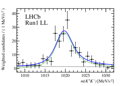
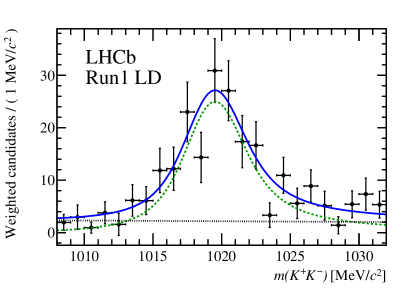
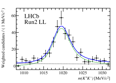
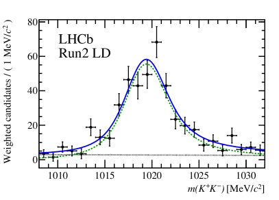
For the normalization channel, the total ${{B}^{0}}\!\rightarrow\phi{{K}^{0}_{\mathrm{S}}}$ yield is obtained from extended unbinned maximum likelihood fits to the reconstructed $B^{0}$ mass in the range , separately for each data sample and reconstruction category. The signal component is modelled by a Hypatia function with power-law tails on both sides [40], where the tail parameters are fixed to values obtained from fits to simulated samples. The mean, width and signal yield parameters are free to vary in the fit. An exponential function with a free slope parameter models the combinatorial background. To account for non-$\phi$ contributions to the ${{B}^{0}}\!\rightarrow\phi{{K}^{0}_{\mathrm{S}}}$ yield, a subsequent fit is performed to the $m({{K}^{+}}{{K}^{-}})$ distribution, which is background-subtracted using the ${}_{s}\mathcal{P}\text{lot}$ technique [41] and where the $m({{K}^{+}}{{K}^{-}}{{K}^{0}_{\mathrm{S}}})$ distribution is used as the discriminating variable. The signal $\phi$ component of the $m({{K}^{+}}{{K}^{-}})$ fit is modelled by a relativistic Breit–Wigner function [42] convolved with a Gaussian function to take into account the resolution of the detector, while the non-$\phi$ contributions are described by an exponential function. The slope parameter of the latter model is Gaussian-constrained to the results obtained from fits to the simulation of $f_{0}(980)\rightarrow{{K}^{+}}{{K}^{-}}$ decays, which is found to better describe the observed distribution than a phase-space model. The measured yields for the normalization channel are shown in the last row of Table 1. Plots of the $m({{K}^{+}}{{K}^{-}}{{K}^{0}_{\mathrm{S}}})$ distributions for the Run 2 LL and LD samples are shown in Figure 1. The remaining $m({{K}^{+}}{{K}^{-}}{{K}^{0}_{\mathrm{S}}})$ distributions and the $m({{K}^{+}}{{K}^{-}})$ distributions are shown in the Appendix.

Figure 1: Fits to the invariant-mass distribution $m({{K}^{0}_{\mathrm{S}}}{{K}^{+}}{{K}^{-}})$ of the normalization decay channel. The black curve represents the complete model, the ${{B}^{0}}\!\rightarrow\phi{{K}^{0}_{\mathrm{S}}}$ component is given in green (dashed), while the background component in shown in red (dotted).

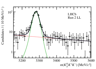
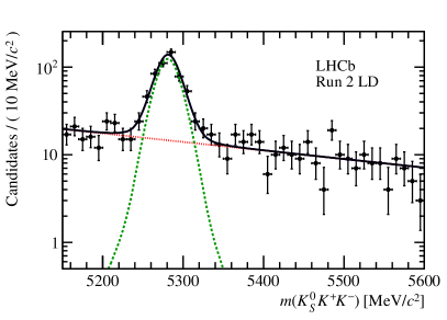
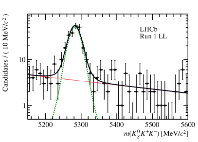
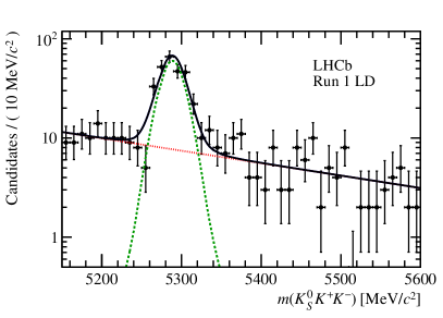
A Hypatia function is used to model the $m({{K}^{0}_{\mathrm{S}}}{{K}^{0}_{\mathrm{S}}})$ distribution of signal ${{B}^{0}_{s}}\!\rightarrow{{K}^{0}_{\mathrm{S}}}{{K}^{0}_{\mathrm{S}}}$ decays. All shape parameters are fixed to values obtained from fits to simulated samples. To account for resolution differences between simulation and data, the width is scaled by a factor—determined from the normalization channel—which takes values in the range 1.05 to 1.20 depending on the data sample. To model the ${{B}^{0}}\!\rightarrow{{K}^{0}_{\mathrm{S}}}{{K}^{0}_{\mathrm{S}}}$ signal component, the same signal shape is duplicated and shifted by the ${{B}^{0}_{s}}-{{B}^{0}}$ mass difference [43]. The background component is modelled by an exponential function with a free slope parameter.

In contrast to the normalization channel, where each data category is fitted individually, a simultaneous fit to the $m({{K}^{0}_{\mathrm{S}}}{{K}^{0}_{\mathrm{S}}})$ distribution of the four data categories (Run 1 LL, Run 1 LD, Run 2 LL, Run 2 LD) is performed in the range . Two parameters are shared across all categories in the simultaneous fit, the ratio of the ${{B}^{0}}\!\rightarrow{{K}^{0}_{\mathrm{S}}}{{K}^{0}_{\mathrm{S}}}$ and ${{B}^{0}_{s}}\!\rightarrow{{K}^{0}_{\mathrm{S}}}{{K}^{0}_{\mathrm{S}}}$ yields $f_{{{B}^{0}}/{{B}^{0}_{s}}}$ and the branching fraction ${\mathcal{B}}(\mbox{${{B}^{0}_{s}}\!\rightarrow{{K}^{0}_{\mathrm{S}}}{{K}^{0}_{\mathrm{S}}}$})$, which is itself related to the signal yield of each data category via the relation

$${\mathcal{B}}(\mbox{${{B}^{0}_{s}}\!\rightarrow{{K}^{0}_{\mathrm{S}}}{{K}^{0}_{\mathrm{S}}}$}) =\frac{\varepsilon_{\phi{{K}^{0}_{\mathrm{S}}},\,i}}{\varepsilon_{{{K}^{0}_{\mathrm{S}}}{{K}^{0}_{\mathrm{S}}},\,i}}\frac{f_{d}}{f_{s}}\frac{{\mathcal{B}}(\mbox{$\phi\!\rightarrow{{K}^{+}}{{K}^{-}}$})}{{\mathcal{B}}(\mbox{${{K}^{0}_{\mathrm{S}}}\!\rightarrow{{\pi}^{+}}{{\pi}^{-}}$})}\frac{{\mathcal{B}}(\mbox{${{B}^{0}}\!\rightarrow\phi{{K}^{0}_{\mathrm{S}}}$})}{N_{i}(\mbox{${{B}^{0}}\!\rightarrow\phi{{K}^{0}_{\mathrm{S}}}$})}\cdot N_{i}(\mbox{${{B}^{0}_{s}}\!\rightarrow{{K}^{0}_{\mathrm{S}}}{{K}^{0}_{\mathrm{S}}}$})$$ (1)

$$\equiv\alpha_{i}\cdot N_{i}(\mbox{${{B}^{0}_{s}}\!\rightarrow{{K}^{0}_{\mathrm{S}}}{{K}^{0}_{\mathrm{S}}}$})\,,$$

where the normalization constant $\alpha_{i}$ is introduced for each data category sample $i$. While the selection efficiencies $\varepsilon$ and signal yields $N$ are determined in the present analysis, external sources are used for the ratio of fragmentation fractions $\nicefrac{{f_{d}}}{{f_{s}}}$ [44, 45], and the branching fractions ${\mathcal{B}}(\mbox{${{B}^{0}}\!\rightarrow\phi{{K}^{0}_{\mathrm{S}}}$})$, ${\mathcal{B}}(\mbox{${{K}^{0}_{\mathrm{S}}}\!\rightarrow{{\pi}^{+}}{{\pi}^{-}}$})$ and ${\mathcal{B}}(\mbox{$\phi\!\rightarrow{{K}^{+}}{{K}^{-}}$})$ [15]. To increase the robustness of the fit, the $\alpha_{i}$ constants are Gaussian constrained within their uncertainties, excluding the uncertainties from the external constants. These external uncertainties are instead applied directly to the final branching ratio measurement.

The efficiency ratio, $\varepsilon_{\phi{{K}^{0}_{\mathrm{S}}}}/\varepsilon_{{{K}^{0}_{\mathrm{S}}}{{K}^{0}_{\mathrm{S}}}}$, is determined from simulation and corrected using data control samples. This ratio is found to be approximately equal to 30 in all data samples except the Run 1 LD sample, where it is twice as large due to lower trigger efficiency for downstream tracks in this sample.

Table 1: Results of the simultaneous fit to the invariant mass of the ${{K}^{0}_{\mathrm{S}}}{{K}^{0}_{\mathrm{S}}}$ system. The fit results for $\mathcal{B}$ and $f_{{{B}^{0}}/{{B}^{0}_{s}}}$ are shared among all data categories. The given uncertainties are statistical only. The normalization constant $\alpha$ and the corresponding normalization channel yields $N_{\text{norm}}$ are shown for reference.

	Run 1 LL	Run 1 LD	Run 2 LL	Run 2 LD	Status
Parameter
$\mathcal{B}$ $(\times 10^{-6})$	8.3 $\pm$ 1.6				Free
$f_{{{B}^{0}}/{{B}^{0}_{s}}}$	0.30 $\pm$ 0.13				Free
$N_{{{B}^{0}_{s}}}$	$4.3\pm\pm 1.0$	$2.1\pm\pm 0.5$	$12.8\pm\pm 2.7$	$12.4\pm\pm 2.7$	${\mathcal{B}}/\alpha$
$N_{{{B}^{0}}}$	$1.3\pm\pm 0.5$	$0.63\pm\pm 0.26$	$3.8\pm\pm 1.5$	$3.7\pm\pm 1.5$	$f_{{{B}^{0}}/{{B}^{0}_{s}}}\times{\mathcal{B}}/\alpha$
$N_{\text{bkg}}$	$10.4\pm\pm 3.5$	$3.5\pm\pm 2.2$	$7.2\pm\pm 3.0$	$13\pm\pm 4$	Free
$\alpha$ $(\times 10^{-6})$	$1.90\pm\pm 0.21$	$3.9\pm\pm 0.5$	$0.65\pm\pm 0.05$	$0.66\pm\pm 0.05$	Gaussian constr.
$N_{\text{norm}}$	$179\pm\pm 18$	$178\pm\pm 22$	$316\pm\pm 25$	$400\pm\pm 31$	Included in $\alpha$

Figure 2: Combined invariant-mass distribution $m({{K}^{0}_{\mathrm{S}}}{{K}^{0}_{\mathrm{S}}})$ of the signal decay channel. The black (solid) curve represents the complete model, the ${B}^{0}_{s}$ signal component is given in green (dashed), the smaller ${B}^{0}$ signal is given in blue (dash-dotted) and the background component in red (dotted).

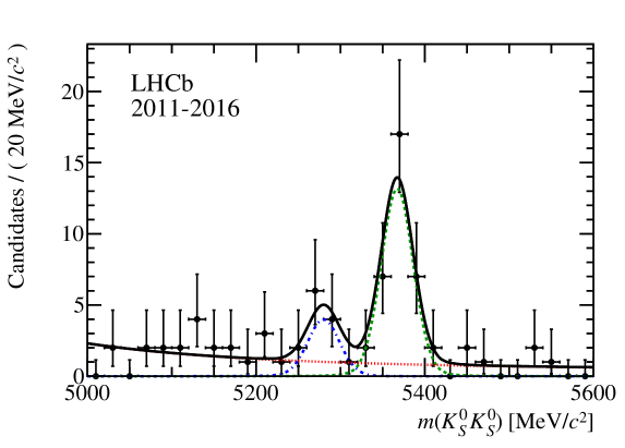
The fit results are shown in Fig. 2. The results of the simultaneous mass fit are given in Table 1, yielding a branching fraction of ${\mathcal{B}}(\mbox{${{B}^{0}_{s}}\!\rightarrow{{K}^{0}_{\mathrm{S}}}{{K}^{0}_{\mathrm{S}}}$})=$(8.3\pm\pm 1.6)\text{\times}{10}^{-6}$$, where the uncertainty is statistical only. The ${{B}^{0}_{s}}\!\rightarrow{{K}^{0}_{\mathrm{S}}}{{K}^{0}_{\mathrm{S}}}$ yield is around 32. The ratio of the branching fractions of the signal and normalization modes ${\mathcal{B}}(\mbox{${{B}^{0}_{s}}\!\rightarrow{{K}^{0}_{\mathrm{S}}}{{K}^{0}_{\mathrm{S}}}$})/{\mathcal{B}}(\mbox{${{B}^{0}}\!\rightarrow\phi{{K}^{0}_{\mathrm{S}}}$})$ can also be calculated by removing the contribution of the world-average value of ${\mathcal{B}}(\mbox{${{B}^{0}}\!\rightarrow\phi{{K}^{0}_{\mathrm{S}}}$})$ from the fit result. This yields a combined branching fraction ratio ${\mathcal{B}}(\mbox{${{B}^{0}_{s}}\!\rightarrow{{K}^{0}_{\mathrm{S}}}{{K}^{0}_{\mathrm{S}}}$})/{\mathcal{B}}(\mbox{${{B}^{0}}\!\rightarrow\phi{{K}^{0}_{\mathrm{S}}}$})=$2.3\pm\pm 0.4$$, where the uncertainty is statistical only.

From the same fit, the relative fraction of ${{B}^{0}}\!\rightarrow{{K}^{0}_{\mathrm{S}}}{{K}^{0}_{\mathrm{S}}}$ decays, $f_{{{B}^{0}}/{{B}^{0}_{s}}}=$0.3\pm\pm 0.13$$ is also determined. Given that the final-state particles and selections applied to the ${K}^{0}_{\mathrm{S}}$ candidates are the same for both modes, the ratio of selection efficiencies is equal to one, so that $f_{{{B}^{0}}/{{B}^{0}_{s}}}$ can be converted to a ratio of branching fractions by multiplying by $\nicefrac{{f_{s}}}{{f_{d}}}$. The calculated value of ${\mathcal{B}}(\mbox{${{B}^{0}}\!\rightarrow{{K}^{0}_{\mathrm{S}}}{{K}^{0}_{\mathrm{S}}}$})/{\mathcal{B}}(\mbox{${{B}^{0}_{s}}\!\rightarrow{{K}^{0}_{\mathrm{S}}}{{K}^{0}_{\mathrm{S}}}$})$ is $(7.5\pm\pm 3.1)\text{\times}{10}^{-2}$, where the uncertainty is statistical only.

The significances of the ${{B}^{0}_{s}}\!\rightarrow{{K}^{0}_{\mathrm{S}}}{{K}^{0}_{\mathrm{S}}}$ and ${{B}^{0}}\!\rightarrow{{K}^{0}_{\mathrm{S}}}{{K}^{0}_{\mathrm{S}}}$ signal yields are estimated relative to a background-only hypothesis using Wilks’ theorem [46]. The observed signal yield of 32 ${{B}^{0}_{s}}\!\rightarrow{{K}^{0}_{\mathrm{S}}}{{K}^{0}_{\mathrm{S}}}$ decays has a large significance of $8.6\text{\,}\sigma$ ($6.5\text{\,}\sigma$ including the effect of systematic uncertainties), while the smaller ${{B}^{0}}\!\rightarrow{{K}^{0}_{\mathrm{S}}}{{K}^{0}_{\mathrm{S}}}$ signal yield has a significance of $3.5\text{\,}\sigma$ including systematic uncertainties.

5 Systematic uncertainties

Each source of systematic uncertainty is evaluated independently and expressed as a relative uncertainty on the branching fraction of ${{B}^{0}_{s}}\!\rightarrow{{K}^{0}_{\mathrm{S}}}{{K}^{0}_{\mathrm{S}}}$ decays. A complete list is given in Table 2. The uncertainties are grouped into three general categories: fit and weighting uncertainties, PID uncertainties, and detector and trigger uncertainties.

Table 2: All systematic uncertainties on the ${{B}^{0}_{s}}\!\rightarrow{{K}^{0}_{\mathrm{S}}}{{K}^{0}_{\mathrm{S}}}$ branching fraction, presented as relative measurements. The last row shows the combined systematic uncertainty for each data sample.

	Run 1, LL	Run 1, LD	Run 2, LL	Run 2, LD
Systematic uncert.
Fit bias	0.059	0.059	0.059	0.059
Fit model choice	0.022	0.033	0.015	0.013
Fit model parameters	0.026	0.026	0.026	0.026
BDT	0.023	0.040	0.014	0.031
PID	0.007	0.008	0.026	0.026
Hardware trigger	0.063	0.062	0.063	0.062
Software trigger	0.065	0.106	0.008	0.026
Trigger misconfig.	—	—	0.007	0.004
${\pi}^{\pm}$/${K}^{\pm}$ hadronic interaction	0.005	0.005	0.005	0.005
VELO misalignment	0.008	0.008	0.008	0.008
Total	0.116	0.149	0.097	0.103

Multiple different fit uncertainties are considered. Uncertainty from possible bias in the combined fit to all four data samples can be estimated using pseudoexperiments generated and fitted according to the default fit model. In each pseudoexperiment, the number of signal candidates is drawn from a Poisson distribution with a mean determined from the baseline fit result. A relative average difference between the generated and fitted branching fraction of $5.9\text{\,}\mathrm{\char 37\relax}$ is determined and conservatively assigned as a systematic uncertainty. The same procedure is performed for the ${{B}^{0}}\!\rightarrow{{K}^{0}_{\mathrm{S}}}{{K}^{0}_{\mathrm{S}}}$ component, yielding a possible bias of $1.6\text{\,}\mathrm{\char 37\relax}$. To ensure a conservative approach, the $5.9\text{\,}\mathrm{\char 37\relax}$ value from ${{B}^{0}_{s}}\!\rightarrow{{K}^{0}_{\mathrm{S}}}{{K}^{0}_{\mathrm{S}}}$ is also applied as the systematic for ${{B}^{0}}\!\rightarrow{{K}^{0}_{\mathrm{S}}}{{K}^{0}_{\mathrm{S}}}$.

Another systematic uncertainty in the fitting process arises from the specific fit model choice, which is quantified by the use of alternative probability density functions to describe the invariant-mass distributions. The reconstructed-mass shapes for ${B}^{0}$ and ${B}^{0}_{s}$ mesons are modelled by the sum of two Crystal Ball functions [47]. For the fit to the $m({{K}^{+}}{{K}^{-}})$ distribution, the $\phi$ meson is modelled by a non-relativistic Breit–Wigner function. For the normalization channel, the relative yield difference when refitting the data is taken as the systematic uncertainty, while for the ${{B}^{0}_{s}}\!\rightarrow{{K}^{0}_{\mathrm{S}}}{{K}^{0}_{\mathrm{S}}}$ decay pseudoexperiments are used to estimate the impact of mismodeling the shape of the signal component. The systematic uncertainty due to the choice of fit model is then the sum in quadrature of these variations, yielding values of $1.3\text{\,}\mathrm{\char 37\relax}$ to $3.3\text{\,}\mathrm{\char 37\relax}$ depending on the data category. Another systematic uncertainty of $2.6\text{\,}\mathrm{\char 37\relax}$, evaluated with a similar procedure, is assigned due to fixing certain shape parameters to values obtained in fits to simulated samples.

Additionally, not all differences between data and simulation can be accounted for using weights in the BDT training. As a conservative upper limit of this effect, the signal efficiency is calculated with and without weights, and the differences between these efficiencies are treated as a systematic uncertainty. This systematic uncertainty is larger by a factor of about 2 for data categories containing a downstream ${K}^{0}_{\mathrm{S}}$ candidate than in those that contain only long ${K}^{0}_{\mathrm{S}}$ candidates, indicating a stronger dependence of the LD channel efficiencies on the weighting.

Three sources of systematic uncertainties from PID efficiencies are considered. The effect of the finite size of the signal simulation samples is evaluated using the bootstrap method [48] for each simulation category and calculating the variance of the signal efficiency. A second systematic uncertainty is calculated by varying the model used to resample PID calibration data, and the relative difference in the signal efficiency is taken as a systematic uncertainty, though this effect is small compared to the previous source. Finally, the flight distance of the ${K}^{0}_{\mathrm{S}}$ candidate is not considered in the resampling process, while the PID efficiency does exhibit some correlation with this variable. A systematic uncertainty is calculated by reweighting the PID distributions in bins of the ${K}^{0}_{\mathrm{S}}$ flight distance, and calculating the relative signal efficiency on resampled simulation and resampled and reweighted simulation. The combined PID systematic uncertainty is given by summing over the three effects in quadrature, which is below $1\text{\,}\mathrm{\char 37\relax}$ for the Run 1 samples and below $3\text{\,}\mathrm{\char 37\relax}$ for the Run 2 samples.

Systematic uncertainties in the trigger system are divided into hardware and software trigger uncertainties. For the hardware trigger stage, the efficiency taken from simulation is compared with data calibration samples. The calibration data is used to correct the simulated efficiencies, and the resulting $6\text{\,}\mathrm{\char 37\relax}$ relative difference in efficiency between the signal and normalization modes is treated as a systematic uncertainty. For the inclusive $B$ software trigger, possible differences in efficiency between the signal and normalization channels are obtained by reweighting the ${{B}^{0}}\!\rightarrow\phi{{K}^{0}_{\mathrm{S}}}$ simulation to match the ${{B}^{0}_{s}}\!\rightarrow{{K}^{0}_{\mathrm{S}}}{{K}^{0}_{\mathrm{S}}}$ simulation and calculating the relative efficiency difference between the raw and reweighted distributions, yielding a systematic uncertainty of about $2\text{\,}\mathrm{\char 37\relax}$. An additional, larger systematic uncertainty is also included to account for the dedicated $\phi$ trigger requirements, which are only used for the normalization channel. Again, weighted ${{B}^{0}}\!\rightarrow\phi{{K}^{0}_{\mathrm{S}}}$ data are used to evaluate a relative efficiency difference between simulation and data, multiplied by the fraction of events solely triggered by the dedicated $\phi$ trigger requirements. The systematic uncertainty is about $5\text{\,}\mathrm{\char 37\relax}10\text{\,}\mathrm{\char 37\relax}$ in Run 1, but about 5 times smaller for Run 2. This is because the topological $b$-hadron trigger is more efficient in Run 2 so that there are far fewer events triggered only by the dedicated $\phi$ trigger. An additional systematic uncertainty less than $1\text{\,}\mathrm{\char 37\relax}$ is assigned to account for a small known misconfiguration of the trigger during Run 2 data taking.

Two additional detector-related uncertainties are considered. A relative uncertainty of $0.5\text{\,}\mathrm{\char 37\relax}$ is assigned due to the different hadronic interaction probabilities between pions and kaons in data and simulation, and a relative uncertainty of $0.8\text{\,}\mathrm{\char 37\relax}$ is also introduced to account for a possible misalignment in the downstream positions of the vertex detector.

The combined systematic uncertainty is determined by using a weighted average of the total systematic uncertainty for each data category, where the weighting is based on the ${B}^{0}_{s}$ signal yield for each category, obtained from the nominal combined fit for the branching fraction. This value is then combined with the systematic uncertainties due to the $\phi\!\rightarrow{{K}^{+}}{{K}^{-}}$ and ${{K}^{0}_{\mathrm{S}}}\!\rightarrow{{\pi}^{+}}{{\pi}^{-}}$ branching fractions, to produce an overall systematic uncertainty of $10.7\text{\,}\mathrm{\char 37\relax}$. The systematic uncertainties due to ${\mathcal{B}}(\mbox{${{B}^{0}}\!\rightarrow\phi{{K}^{0}_{\mathrm{S}}}$})$ or $\nicefrac{{f_{s}}}{{f_{d}}}$ are provided separately when necessary. The total systematic uncertainty in the measurement of the ${B}^{0}$ branching fraction is also $10.7\text{\,}\mathrm{\char 37\relax}$.

These measurements of the branching ratio are calculated using the time-integrated event yield, without taking into account ${B}^{0}_{s}$–${\kern 1.79993pt\overline{\kern-1.79993ptB}{}}{}^{0}_{s}$ mixing effects. The conversion into a branching ratio that is independent of ${B}^{0}_{s}$–${\kern 1.79993pt\overline{\kern-1.79993ptB}{}}{}^{0}_{s}$ mixing can be performed according to the computation given in Ref. [49], where $\mathcal{A}^{f}_{\Delta\Gamma}$ is calculated from the decay amplitudes of the $B_{s}^{\text{H}}$ and $B_{s}^{\text{L}}$ states. In this work, the simulation is generated using the average ${B}^{0}_{s}$ lifetime, corresponding to the $\mathcal{A}^{f}_{\Delta\Gamma}=0$ scenario. For this scenario the mixing-corrected SM prediction of the branching ratio is equivalent to the quoted time-integrated branching ratio within uncertainties, because the impact of the scaling from $\Delta\Gamma_{s}/\Gamma_{s}=0.135\pm 0.008$ [15] is small.

Considering that the final state of the decay is $C\!P$-even, the relevant decay lifetime of the ${B}^{0}_{s}$ is expected to be closer to that of the $B_{s}^{\text{L}}$ state, corresponding to a SM prediction of $\mathcal{A}^{f}_{\Delta\Gamma}$ close to $-1$. This change in lifetime corresponds to a change in the expected efficiency of the ${{B}^{0}_{s}}\!\rightarrow{{K}^{0}_{\mathrm{S}}}{{K}^{0}_{\mathrm{S}}}$ reconstruction of approximately $-4.5\text{\,}\mathrm{\char 37\relax}$ for $\mathcal{A}^{f}_{\Delta\Gamma}=-1$, or $4.5\text{\,}\mathrm{\char 37\relax}$ for the less-likely $\mathcal{A}^{f}_{\Delta\Gamma}=1$. These scaling factors are not included in the systematic uncertainty for the time-integrated branching ratios presented below.

6 Conclusion

Data collected by the LHCb experiment in 2011–2012 and 2015–2016 was used to measure the ${{B}^{0}_{s}}\!\rightarrow{{K}^{0}_{\mathrm{S}}}{{K}^{0}_{\mathrm{S}}}$ branching fraction. The measured ratio of this branching fraction relative to that of the normalization channel is

$$\frac{{\mathcal{B}}(\mbox{${{B}^{0}_{s}}\!\rightarrow{{K}^{0}_{\mathrm{S}}}{{K}^{0}_{\mathrm{S}}}$})}{{\mathcal{B}}(\mbox{${{B}^{0}}\!\rightarrow\phi{{K}^{0}_{\mathrm{S}}}$})}=2.3\pm 0.4\,(\text{stat})\pm 0.2\,(\text{syst})\pm 0.1\,(\nicefrac{{f_{s}}}{{f_{d}}}),$$

where the first uncertainty is statistical, the second is systematic, and the third is due to the ratio of hadronization fractions. This is compatible with the ratio ${\mathcal{B}}(\mbox{${{B}^{0}_{s}}\!\rightarrow{{K}^{0}_{\mathrm{S}}}{{K}^{0}_{\mathrm{S}}}$})/{\mathcal{B}}(\mbox{${{B}^{0}}\!\rightarrow\phi{{K}^{0}_{\mathrm{S}}}$})=2.7\pm 0.9$ calculated from the current world average values [15].

From this measurement, the ${{B}^{0}_{s}}\!\rightarrow{{K}^{0}_{\mathrm{S}}}{{K}^{0}_{\mathrm{S}}}$ branching fraction is determined to be

$${\mathcal{B}}(\mbox{${{B}^{0}_{s}}\!\rightarrow{{K}^{0}_{\mathrm{S}}}{{K}^{0}_{\mathrm{S}}}$})=[8.3\pm 1.6\,(\text{stat})\pm 0.9\,(\text{syst})\pm 0.8\,(\text{norm})\pm 0.3\,(\nicefrac{{f_{s}}}{{f_{d}}})]\times 10^{-6},$$

where the first uncertainty is statistical, the second is systematic, and the third and fourth are due to the normalization channel branching fraction and the ratio of hadronization fractions $\nicefrac{{f_{s}}}{{f_{d}}}$. This result is the most precise to date and is compatible with SM predictions [6, 7, 8, 9] and the previous measurement from the Belle collaboration [14].

In the same combined fit used for the ${{B}^{0}_{s}}\!\rightarrow{{K}^{0}_{\mathrm{S}}}{{K}^{0}_{\mathrm{S}}}$ measurement, the fraction of ${{B}^{0}}\!\rightarrow{{K}^{0}_{\mathrm{S}}}{{K}^{0}_{\mathrm{S}}}$ decays is also determined. Using this measured fraction of yields, the branching fraction of ${{B}^{0}}\!\rightarrow{{K}^{0}_{\mathrm{S}}}{{K}^{0}_{\mathrm{S}}}$ decays measured relative to ${{B}^{0}_{s}}\!\rightarrow{{K}^{0}_{\mathrm{S}}}{{K}^{0}_{\mathrm{S}}}$ decays is found to be

$$\frac{{\mathcal{B}}(\mbox{${{B}^{0}}\!\rightarrow{{K}^{0}_{\mathrm{S}}}{{K}^{0}_{\mathrm{S}}}$})}{{\mathcal{B}}(\mbox{${{B}^{0}_{s}}\!\rightarrow{{K}^{0}_{\mathrm{S}}}{{K}^{0}_{\mathrm{S}}}$})}=[7.5\pm 3.1\,(\text{stat})\pm 0.5\,(\text{syst})\pm 0.3\,(\nicefrac{{f_{s}}}{{f_{d}}})]\times 10^{-2},$$

where the first uncertainty is statistical, the second is systematic, and the third is due to the ratio of hadronization fractions. For comparison, calculating ${\mathcal{B}}(\mbox{${{B}^{0}}\!\rightarrow{{K}^{0}_{\mathrm{S}}}{{K}^{0}_{\mathrm{S}}}$})/{\mathcal{B}}(\mbox{${{B}^{0}_{s}}\!\rightarrow{{K}^{0}_{\mathrm{S}}}{{K}^{0}_{\mathrm{S}}}$})$ based on world average-values [15] yields $(6.0\pm 2.0)\%$, which is compatible with the obtained result.

The ${{B}^{0}}\!\rightarrow{{K}^{0}_{\mathrm{S}}}{{K}^{0}_{\mathrm{S}}}$ branching fraction relative to the ${{B}^{0}}\!\rightarrow\phi{{K}^{0}_{\mathrm{S}}}$ normalization mode is determined to be

$$\frac{{\mathcal{B}}(\mbox{${{B}^{0}}\!\rightarrow{{K}^{0}_{\mathrm{S}}}{{K}^{0}_{\mathrm{S}}}$})}{{\mathcal{B}}(\mbox{${{B}^{0}}\!\rightarrow\phi{{K}^{0}_{\mathrm{S}}}$})}=0.17\pm 0.08\,(\text{stat})\pm 0.02\,(\text{syst}),$$

where the first uncertainty is statistical, and the second is systematic.

Appendix: Normalization channel fits

Figure 3 shows the $m({{K}^{0}_{\mathrm{S}}}{{K}^{+}}{{K}^{-}})$ distributions for the Run 1 LL and LD categories. The $m({{K}^{+}}{{K}^{-}})$ distributions for all four data categories are shown in Fig. 4.

Figure 3: Fits to the invariant-mass distribution $m({{K}^{0}_{\mathrm{S}}}{{K}^{+}}{{K}^{-}})$ of the normalization decay channel. The black curve represents the complete model, the ${{B}^{0}}\!\rightarrow\phi{{K}^{0}_{\mathrm{S}}}$ component is given in green (dashed), while the background component in shown in red (dotted).

Figure 4: Fits to the invariant-mass distribution $m({{K}^{+}}{{K}^{-}})$ of ${{B}^{0}}\!\rightarrow\phi{{K}^{0}_{\mathrm{S}}}$ data weighted using the ${}_{s}\mathcal{P}\text{lot}$ technique. The blue curve represents the complete model, the signal $\phi$ component is given in green (dashed), and the background $f_{0}(980)\rightarrow{{K}^{+}}{{K}^{-}}$ model is shown in black (dotted).

LHCb collaboration

R. Aaij³¹, C. Abellán Beteta⁴⁹, T. Ackernley⁵⁹, B. Adeva⁴⁵, M. Adinolfi⁵³, H. Afsharnia⁹, C.A. Aidala⁷⁹, S. Aiola²⁵, Z. Ajaltouni⁹, S. Akar⁶⁴, P. Albicocco²², J. Albrecht¹⁴, F. Alessio⁴⁷, M. Alexander⁵⁸, A. Alfonso Albero⁴⁴, G. Alkhazov³⁷, P. Alvarez Cartelle⁶⁰, A.A. Alves Jr⁴⁵, S. Amato², Y. Amhis¹¹, L. An²¹, L. Anderlini²¹, G. Andreassi⁴⁸, M. Andreotti²⁰, F. Archilli¹⁶, J. Arnau Romeu¹⁰, A. Artamonov⁴³, M. Artuso⁶⁷, K. Arzymatov⁴¹, E. Aslanides¹⁰, M. Atzeni⁴⁹, B. Audurier²⁶, S. Bachmann¹⁶, J.J. Back⁵⁵, S. Baker⁶⁰, V. Balagura^11,b, W. Baldini^20,47, A. Baranov⁴¹, R.J. Barlow⁶¹, S. Barsuk¹¹, W. Barter⁶⁰, M. Bartolini^23,47,h, F. Baryshnikov⁷⁶, G. Bassi²⁸, V. Batozskaya³⁵, B. Batsukh⁶⁷, A. Battig¹⁴, V. Battista⁴⁸, A. Bay⁴⁸, M. Becker¹⁴, F. Bedeschi²⁸, I. Bediaga¹, A. Beiter⁶⁷, L.J. Bel³¹, V. Belavin⁴¹, S. Belin²⁶, N. Beliy⁵, V. Bellee⁴⁸, K. Belous⁴³, I. Belyaev³⁸, G. Bencivenni²², E. Ben-Haim¹², S. Benson³¹, S. Beranek¹³, A. Berezhnoy³⁹, R. Bernet⁴⁹, D. Berninghoff¹⁶, H.C. Bernstein⁶⁷, E. Bertholet¹², A. Bertolin²⁷, C. Betancourt⁴⁹, F. Betti^19,e, M.O. Bettler⁵⁴, Ia. Bezshyiko⁴⁹, S. Bhasin⁵³, J. Bhom³³, M.S. Bieker¹⁴, S. Bifani⁵², P. Billoir¹², A. Bizzeti^21,u, M. Bjørn⁶², M.P. Blago⁴⁷, T. Blake⁵⁵, F. Blanc⁴⁸, S. Blusk⁶⁷, D. Bobulska⁵⁸, V. Bocci³⁰, O. Boente Garcia⁴⁵, T. Boettcher⁶³, A. Boldyrev⁷⁷, A. Bondar^42,x, N. Bondar³⁷, S. Borghi^61,47, M. Borisyak⁴¹, M. Borsato¹⁶, J.T. Borsuk³³, T.J.V. Bowcock⁵⁹, C. Bozzi²⁰, S. Braun¹⁶, A. Brea Rodriguez⁴⁵, M. Brodski⁴⁷, J. Brodzicka³³, A. Brossa Gonzalo⁵⁵, D. Brundu²⁶, E. Buchanan⁵³, A. Büchler-Germann⁴⁹, A. Buonaura⁴⁹, C. Burr⁴⁷, A. Bursche²⁶, J.S. Butter³¹, J. Buytaert⁴⁷, W. Byczynski⁴⁷, S. Cadeddu²⁶, H. Cai⁷¹, R. Calabrese^20,g, S. Cali²², R. Calladine⁵², M. Calvi^24,i, M. Calvo Gomez^44,m, A. Camboni^44,m, P. Campana²², D.H. Campora Perez⁴⁷, L. Capriotti^19,e, A. Carbone^19,e, G. Carboni²⁹, R. Cardinale^23,h, A. Cardini²⁶, P. Carniti^24,i, K. Carvalho Akiba³¹, A. Casais Vidal⁴⁵, G. Casse⁵⁹, M. Cattaneo⁴⁷, G. Cavallero⁴⁷, R. Cenci^28,p, J. Cerasoli¹⁰, M.G. Chapman⁵³, M. Charles^12,47, Ph. Charpentier⁴⁷, G. Chatzikonstantinidis⁵², M. Chefdeville⁸, V. Chekalina⁴¹, C. Chen³, S. Chen²⁶, A. Chernov³³, S.-G. Chitic⁴⁷, V. Chobanova⁴⁵, M. Chrzaszcz⁴⁷, A. Chubykin³⁷, P. Ciambrone²², M.F. Cicala⁵⁵, X. Cid Vidal⁴⁵, G. Ciezarek⁴⁷, F. Cindolo¹⁹, P.E.L. Clarke⁵⁷, M. Clemencic⁴⁷, H.V. Cliff⁵⁴, J. Closier⁴⁷, J.L. Cobbledick⁶¹, V. Coco⁴⁷, J.A.B. Coelho¹¹, J. Cogan¹⁰, E. Cogneras⁹, L. Cojocariu³⁶, P. Collins⁴⁷, T. Colombo⁴⁷, A. Comerma-Montells¹⁶, A. Contu²⁶, N. Cooke⁵², G. Coombs⁵⁸, S. Coquereau⁴⁴, G. Corti⁴⁷, C.M. Costa Sobral⁵⁵, B. Couturier⁴⁷, D.C. Craik⁶³, J. Crkovská⁶⁶, A. Crocombe⁵⁵, M. Cruz Torres^1,ab, R. Currie⁵⁷, C.L. Da Silva⁶⁶, E. Dall’Occo³¹, J. Dalseno^45,53, C. D’Ambrosio⁴⁷, A. Danilina³⁸, P. d’Argent¹⁶, A. Davis⁶¹, O. De Aguiar Francisco⁴⁷, K. De Bruyn⁴⁷, S. De Capua⁶¹, M. De Cian⁴⁸, J.M. De Miranda¹, L. De Paula², M. De Serio^18,d, P. De Simone²², J.A. de Vries³¹, C.T. Dean⁶⁶, W. Dean⁷⁹, D. Decamp⁸, L. Del Buono¹², B. Delaney⁵⁴, H.-P. Dembinski¹⁵, M. Demmer¹⁴, A. Dendek³⁴, V. Denysenko⁴⁹, D. Derkach⁷⁷, O. Deschamps⁹, F. Desse¹¹, F. Dettori^26,f, B. Dey⁷, A. Di Canto⁴⁷, P. Di Nezza²², S. Didenko⁷⁶, H. Dijkstra⁴⁷, F. Dordei²⁶, M. Dorigo^28,y, A.C. dos Reis¹, L. Douglas⁵⁸, A. Dovbnya⁵⁰, K. Dreimanis⁵⁹, M.W. Dudek³³, L. Dufour⁴⁷, G. Dujany¹², P. Durante⁴⁷, J.M. Durham⁶⁶, D. Dutta⁶¹, R. Dzhelyadin^43,†, M. Dziewiecki¹⁶, A. Dziurda³³, A. Dzyuba³⁷, S. Easo⁵⁶, U. Egede⁶⁰, V. Egorychev³⁸, S. Eidelman^42,x, S. Eisenhardt⁵⁷, R. Ekelhof¹⁴, S. Ek-In⁴⁸, L. Eklund⁵⁸, S. Ely⁶⁷, A. Ene³⁶, S. Escher¹³, S. Esen³¹, T. Evans⁴⁷, A. Falabella¹⁹, J. Fan³, N. Farley⁵², S. Farry⁵⁹, D. Fazzini¹¹, M. Féo⁴⁷, P. Fernandez Declara⁴⁷, A. Fernandez Prieto⁴⁵, F. Ferrari^19,e, L. Ferreira Lopes⁴⁸, F. Ferreira Rodrigues², S. Ferreres Sole³¹, M. Ferrillo⁴⁹, M. Ferro-Luzzi⁴⁷, S. Filippov⁴⁰, R.A. Fini¹⁸, M. Fiorini^20,g, M. Firlej³⁴, K.M. Fischer⁶², C. Fitzpatrick⁴⁷, T. Fiutowski³⁴, F. Fleuret^11,b, M. Fontana⁴⁷, F. Fontanelli^23,h, R. Forty⁴⁷, V. Franco Lima⁵⁹, M. Franco Sevilla⁶⁵, M. Frank⁴⁷, C. Frei⁴⁷, D.A. Friday⁵⁸, J. Fu^25,q, Q. Fuehring¹⁴, W. Funk⁴⁷, E. Gabriel⁵⁷, A. Gallas Torreira⁴⁵, D. Galli^19,e, S. Gallorini²⁷, S. Gambetta⁵⁷, Y. Gan³, M. Gandelman², P. Gandini²⁵, Y. Gao⁴, L.M. Garcia Martin⁴⁶, J. García Pardiñas⁴⁹, B. Garcia Plana⁴⁵, F.A. Garcia Rosales¹¹, J. Garra Tico⁵⁴, L. Garrido⁴⁴, D. Gascon⁴⁴, C. Gaspar⁴⁷, D. Gerick¹⁶, E. Gersabeck⁶¹, M. Gersabeck⁶¹, T. Gershon⁵⁵, D. Gerstel¹⁰, Ph. Ghez⁸, V. Gibson⁵⁴, A. Gioventù⁴⁵, O.G. Girard⁴⁸, P. Gironella Gironell⁴⁴, L. Giubega³⁶, C. Giugliano²⁰, K. Gizdov⁵⁷, V.V. Gligorov¹², C. Göbel⁶⁹, E. Golobardes^44,m, D. Golubkov³⁸, A. Golutvin^60,76, A. Gomes^1,a, P. Gorbounov^38,6, I.V. Gorelov³⁹, C. Gotti^24,i, E. Govorkova³¹, J.P. Grabowski¹⁶, R. Graciani Diaz⁴⁴, T. Grammatico¹², L.A. Granado Cardoso⁴⁷, E. Graugés⁴⁴, E. Graverini⁴⁸, G. Graziani²¹, A. Grecu³⁶, R. Greim³¹, P. Griffith²⁰, L. Grillo⁶¹, L. Gruber⁴⁷, B.R. Gruberg Cazon⁶², C. Gu³, E. Gushchin⁴⁰, A. Guth¹³, Yu. Guz^43,47, T. Gys⁴⁷, T. Hadavizadeh⁶², G. Haefeli⁴⁸, C. Haen⁴⁷, S.C. Haines⁵⁴, P.M. Hamilton⁶⁵, Q. Han⁷, X. Han¹⁶, T.H. Hancock⁶², S. Hansmann-Menzemer¹⁶, N. Harnew⁶², T. Harrison⁵⁹, R. Hart³¹, C. Hasse⁴⁷, M. Hatch⁴⁷, J. He⁵, M. Hecker⁶⁰, K. Heijhoff³¹, K. Heinicke¹⁴, A. Heister¹⁴, A.M. Hennequin⁴⁷, K. Hennessy⁵⁹, L. Henry⁴⁶, J. Heuel¹³, A. Hicheur⁶⁸, R. Hidalgo Charman⁶¹, D. Hill⁶², M. Hilton⁶¹, S. Hollitt¹⁴, P.H. Hopchev⁴⁸, J. Hu¹⁶, W. Hu⁷, W. Huang⁵, Z.C. Huard⁶⁴, W. Hulsbergen³¹, T. Humair⁶⁰, R.J. Hunter⁵⁵, M. Hushchyn⁷⁷, D. Hutchcroft⁵⁹, D. Hynds³¹, P. Ibis¹⁴, M. Idzik³⁴, P. Ilten⁵², A. Inglessi³⁷, A. Inyakin⁴³, K. Ivshin³⁷, R. Jacobsson⁴⁷, S. Jakobsen⁴⁷, J. Jalocha⁶², E. Jans³¹, B.K. Jashal⁴⁶, A. Jawahery⁶⁵, V. Jevtic¹⁴, F. Jiang³, M. John⁶², D. Johnson⁴⁷, C.R. Jones⁵⁴, B. Jost⁴⁷, N. Jurik⁶², S. Kandybei⁵⁰, M. Karacson⁴⁷, J.M. Kariuki⁵³, N. Kazeev⁷⁷, M. Kecke¹⁶, F. Keizer⁵⁴, M. Kelsey⁶⁷, M. Kenzie⁵⁴, T. Ketel³², B. Khanji⁴⁷, A. Kharisova⁷⁸, K.E. Kim⁶⁷, T. Kirn¹³, V.S. Kirsebom⁴⁸, S. Klaver²², K. Klimaszewski³⁵, S. Koliiev⁵¹, A. Kondybayeva⁷⁶, A. Konoplyannikov³⁸, P. Kopciewicz³⁴, R. Kopecna¹⁶, P. Koppenburg³¹, M. Korolev³⁹, I. Kostiuk^31,51, O. Kot⁵¹, S. Kotriakhova³⁷, L. Kravchuk⁴⁰, R.D. Krawczyk⁴⁷, M. Kreps⁵⁵, F. Kress⁶⁰, S. Kretzschmar¹³, P. Krokovny^42,x, W. Krupa³⁴, W. Krzemien³⁵, W. Kucewicz^33,l, M. Kucharczyk³³, V. Kudryavtsev^42,x, H.S. Kuindersma³¹, G.J. Kunde⁶⁶, A.K. Kuonen⁴⁸, T. Kvaratskheliya³⁸, D. Lacarrere⁴⁷, G. Lafferty⁶¹, A. Lai²⁶, D. Lancierini⁴⁹, J.J. Lane⁶¹, G. Lanfranchi²², C. Langenbruch¹³, T. Latham⁵⁵, F. Lazzari^28,v, C. Lazzeroni⁵², R. Le Gac¹⁰, R. Lefèvre⁹, A. Leflat³⁹, F. Lemaitre⁴⁷, O. Leroy¹⁰, T. Lesiak³³, B. Leverington¹⁶, H. Li⁷⁰, X. Li⁶⁶, Y. Li⁶, Z. Li⁶⁷, X. Liang⁶⁷, R. Lindner⁴⁷, F. Lionetto⁴⁹, V. Lisovskyi¹¹, G. Liu⁷⁰, X. Liu³, D. Loh⁵⁵, A. Loi²⁶, J. Lomba Castro⁴⁵, I. Longstaff⁵⁸, J.H. Lopes², G. Loustau⁴⁹, G.H. Lovell⁵⁴, Y. Lu⁶, D. Lucchesi^27,o, M. Lucio Martinez³¹, Y. Luo³, A. Lupato²⁷, E. Luppi^20,g, O. Lupton⁵⁵, A. Lusiani^28,t, X. Lyu⁵, S. Maccolini^19,e, F. Machefert¹¹, F. Maciuc³⁶, V. Macko⁴⁸, P. Mackowiak¹⁴, S. Maddrell-Mander⁵³, L.R. Madhan Mohan⁵³, O. Maev^37,47, A. Maevskiy⁷⁷, K. Maguire⁶¹, D. Maisuzenko³⁷, M.W. Majewski³⁴, S. Malde⁶², B. Malecki⁴⁷, A. Malinin⁷⁵, T. Maltsev^42,x, H. Malygina¹⁶, G. Manca^26,f, G. Mancinelli¹⁰, R. Manera Escalero⁴⁴, D. Manuzzi^19,e, D. Marangotto^25,q, J. Maratas^9,w, J.F. Marchand⁸, U. Marconi¹⁹, S. Mariani²¹, C. Marin Benito¹¹, M. Marinangeli⁴⁸, P. Marino⁴⁸, J. Marks¹⁶, P.J. Marshall⁵⁹, G. Martellotti³⁰, L. Martinazzoli⁴⁷, M. Martinelli^24,i, D. Martinez Santos⁴⁵, F. Martinez Vidal⁴⁶, A. Massafferri¹, M. Materok¹³, R. Matev⁴⁷, A. Mathad⁴⁹, Z. Mathe⁴⁷, V. Matiunin³⁸, C. Matteuzzi²⁴, K.R. Mattioli⁷⁹, A. Mauri⁴⁹, E. Maurice^11,b, M. McCann^60,47, L. Mcconnell¹⁷, A. McNab⁶¹, R. McNulty¹⁷, J.V. Mead⁵⁹, B. Meadows⁶⁴, C. Meaux¹⁰, G. Meier¹⁴, N. Meinert⁷³, D. Melnychuk³⁵, S. Meloni^24,i, M. Merk³¹, A. Merli²⁵, M. Mikhasenko⁴⁷, D.A. Milanes⁷², E. Millard⁵⁵, M.-N. Minard⁸, O. Mineev³⁸, L. Minzoni^20,g, S.E. Mitchell⁵⁷, B. Mitreska⁶¹, D.S. Mitzel⁴⁷, A. Mödden¹⁴, A. Mogini¹², R.D. Moise⁶⁰, T. Mombächer¹⁴, I.A. Monroy⁷², S. Monteil⁹, M. Morandin²⁷, G. Morello²², M.J. Morello^28,t, J. Moron³⁴, A.B. Morris¹⁰, A.G. Morris⁵⁵, R. Mountain⁶⁷, H. Mu³, F. Muheim⁵⁷, M. Mukherjee⁷, M. Mulder³¹, D. Müller⁴⁷, K. Müller⁴⁹, V. Müller¹⁴, C.H. Murphy⁶², D. Murray⁶¹, P. Muzzetto²⁶, P. Naik⁵³, T. Nakada⁴⁸, R. Nandakumar⁵⁶, A. Nandi⁶², T. Nanut⁴⁸, I. Nasteva², M. Needham⁵⁷, N. Neri^25,q, S. Neubert¹⁶, N. Neufeld⁴⁷, R. Newcombe⁶⁰, T.D. Nguyen⁴⁸, C. Nguyen-Mau^48,n, E.M. Niel¹¹, S. Nieswand¹³, N. Nikitin³⁹, N.S. Nolte⁴⁷, A. Oblakowska-Mucha³⁴, V. Obraztsov⁴³, S. Ogilvy⁵⁸, D.P. O’Hanlon¹⁹, R. Oldeman^26,f, C.J.G. Onderwater⁷⁴, J. D. Osborn⁷⁹, A. Ossowska³³, J.M. Otalora Goicochea², T. Ovsiannikova³⁸, P. Owen⁴⁹, A. Oyanguren⁴⁶, P.R. Pais⁴⁸, T. Pajero^28,t, A. Palano¹⁸, M. Palutan²², G. Panshin⁷⁸, A. Papanestis⁵⁶, M. Pappagallo⁵⁷, L.L. Pappalardo^20,g, W. Parker⁶⁵, C. Parkes^61,47, G. Passaleva^21,47, A. Pastore¹⁸, M. Patel⁶⁰, C. Patrignani^19,e, A. Pearce⁴⁷, A. Pellegrino³¹, M. Pepe Altarelli⁴⁷, S. Perazzini¹⁹, D. Pereima³⁸, P. Perret⁹, L. Pescatore⁴⁸, K. Petridis⁵³, A. Petrolini^23,h, A. Petrov⁷⁵, S. Petrucci⁵⁷, M. Petruzzo^25,q, B. Pietrzyk⁸, G. Pietrzyk⁴⁸, M. Pikies³³, M. Pili⁶², D. Pinci³⁰, J. Pinzino⁴⁷, F. Pisani⁴⁷, A. Piucci¹⁶, V. Placinta³⁶, S. Playfer⁵⁷, J. Plews⁵², M. Plo Casasus⁴⁵, F. Polci¹², M. Poli Lener²², M. Poliakova⁶⁷, A. Poluektov¹⁰, N. Polukhina^76,c, I. Polyakov⁶⁷, E. Polycarpo², G.J. Pomery⁵³, S. Ponce⁴⁷, A. Popov⁴³, D. Popov⁵², S. Poslavskii⁴³, K. Prasanth³³, L. Promberger⁴⁷, C. Prouve⁴⁵, V. Pugatch⁵¹, A. Puig Navarro⁴⁹, H. Pullen⁶², G. Punzi^28,p, W. Qian⁵, J. Qin⁵, R. Quagliani¹², B. Quintana⁹, N.V. Raab¹⁷, R.I. Rabadan Trejo¹⁰, B. Rachwal³⁴, J.H. Rademacker⁵³, M. Rama²⁸, M. Ramos Pernas⁴⁵, M.S. Rangel², F. Ratnikov^41,77, G. Raven³², M. Ravonel Salzgeber⁴⁷, M. Reboud⁸, F. Redi⁴⁸, S. Reichert¹⁴, F. Reiss¹², C. Remon Alepuz⁴⁶, Z. Ren³, V. Renaudin⁶², S. Ricciardi⁵⁶, S. Richards⁵³, K. Rinnert⁵⁹, P. Robbe¹¹, A. Robert¹², A.B. Rodrigues⁴⁸, E. Rodrigues⁶⁴, J.A. Rodriguez Lopez⁷², M. Roehrken⁴⁷, S. Roiser⁴⁷, A. Rollings⁶², V. Romanovskiy⁴³, M. Romero Lamas⁴⁵, A. Romero Vidal⁴⁵, J.D. Roth⁷⁹, M. Rotondo²², M.S. Rudolph⁶⁷, T. Ruf⁴⁷, J. Ruiz Vidal⁴⁶, J. Ryzka³⁴, J.J. Saborido Silva⁴⁵, N. Sagidova³⁷, B. Saitta^26,f, C. Sanchez Gras³¹, C. Sanchez Mayordomo⁴⁶, B. Sanmartin Sedes⁴⁵, R. Santacesaria³⁰, C. Santamarina Rios⁴⁵, M. Santimaria²², E. Santovetti^29,j, G. Sarpis⁶¹, A. Sarti³⁰, C. Satriano^30,s, A. Satta²⁹, M. Saur⁵, D. Savrina^38,39, L.G. Scantlebury Smead⁶², S. Schael¹³, M. Schellenberg¹⁴, M. Schiller⁵⁸, H. Schindler⁴⁷, M. Schmelling¹⁵, T. Schmelzer¹⁴, B. Schmidt⁴⁷, O. Schneider⁴⁸, A. Schopper⁴⁷, H.F. Schreiner⁶⁴, M. Schubiger³¹, S. Schulte⁴⁸, M.H. Schune¹¹, R. Schwemmer⁴⁷, B. Sciascia²², A. Sciubba^30,k, S. Sellam⁶⁸, A. Semennikov³⁸, A. Sergi^52,47, N. Serra⁴⁹, J. Serrano¹⁰, L. Sestini²⁷, A. Seuthe¹⁴, P. Seyfert⁴⁷, D.M. Shangase⁷⁹, M. Shapkin⁴³, T. Shears⁵⁹, L. Shekhtman^42,x, V. Shevchenko^75,76, E. Shmanin⁷⁶, J.D. Shupperd⁶⁷, B.G. Siddi²⁰, R. Silva Coutinho⁴⁹, L. Silva de Oliveira², G. Simi^27,o, S. Simone^18,d, I. Skiba²⁰, N. Skidmore¹⁶, T. Skwarnicki⁶⁷, M.W. Slater⁵², J.G. Smeaton⁵⁴, A. Smetkina³⁸, E. Smith¹³, I.T. Smith⁵⁷, M. Smith⁶⁰, A. Snoch³¹, M. Soares¹⁹, L. Soares Lavra¹, M.D. Sokoloff⁶⁴, F.J.P. Soler⁵⁸, B. Souza De Paula², B. Spaan¹⁴, E. Spadaro Norella^25,q, P. Spradlin⁵⁸, F. Stagni⁴⁷, M. Stahl⁶⁴, S. Stahl⁴⁷, P. Stefko⁴⁸, S. Stefkova⁶⁰, O. Steinkamp⁴⁹, S. Stemmle¹⁶, O. Stenyakin⁴³, M. Stepanova³⁷, H. Stevens¹⁴, S. Stone⁶⁷, S. Stracka²⁸, M.E. Stramaglia⁴⁸, M. Straticiuc³⁶, S. Strokov⁷⁸, J. Sun³, L. Sun⁷¹, Y. Sun⁶⁵, P. Svihra⁶¹, K. Swientek³⁴, A. Szabelski³⁵, T. Szumlak³⁴, M. Szymanski⁵, S. Taneja⁶¹, Z. Tang³, T. Tekampe¹⁴, G. Tellarini²⁰, F. Teubert⁴⁷, E. Thomas⁴⁷, K.A. Thomson⁵⁹, M.J. Tilley⁶⁰, V. Tisserand⁹, S. T’Jampens⁸, M. Tobin⁶, S. Tolk⁴⁷, L. Tomassetti^20,g, D. Tonelli²⁸, D.Y. Tou¹², E. Tournefier⁸, M. Traill⁵⁸, M.T. Tran⁴⁸, A. Trisovic⁵⁴, A. Tsaregorodtsev¹⁰, G. Tuci^28,47,p, A. Tully⁴⁸, N. Tuning³¹, A. Ukleja³⁵, A. Usachov¹¹, A. Ustyuzhanin^41,77, U. Uwer¹⁶, A. Vagner⁷⁸, V. Vagnoni¹⁹, A. Valassi⁴⁷, G. Valenti¹⁹, M. van Beuzekom³¹, H. Van Hecke⁶⁶, E. van Herwijnen⁴⁷, C.B. Van Hulse¹⁷, J. van Tilburg³¹, M. van Veghel⁷⁴, R. Vazquez Gomez^44,22, P. Vazquez Regueiro⁴⁵, C. Vázquez Sierra³¹, S. Vecchi²⁰, J.J. Velthuis⁵³, M. Veltri^21,r, A. Venkateswaran⁶⁷, M. Vernet⁹, M. Veronesi³¹, M. Vesterinen⁵⁵, J.V. Viana Barbosa⁴⁷, D. Vieira⁵, M. Vieites Diaz⁴⁸, H. Viemann⁷³, X. Vilasis-Cardona^44,m, A. Vitkovskiy³¹, A. Vollhardt⁴⁹, D. Vom Bruch¹², A. Vorobyev³⁷, V. Vorobyev^42,x, N. Voropaev³⁷, R. Waldi⁷³, J. Walsh²⁸, J. Wang³, J. Wang⁷¹, J. Wang⁶, M. Wang³, Y. Wang⁷, Z. Wang⁴⁹, D.R. Ward⁵⁴, H.M. Wark⁵⁹, N.K. Watson⁵², D. Websdale⁶⁰, A. Weiden⁴⁹, C. Weisser⁶³, B.D.C. Westhenry⁵³, D.J. White⁶¹, M. Whitehead¹³, D. Wiedner¹⁴, G. Wilkinson⁶², M. Wilkinson⁶⁷, I. Williams⁵⁴, M. Williams⁶³, M.R.J. Williams⁶¹, T. Williams⁵², F.F. Wilson⁵⁶, M. Winn¹¹, W. Wislicki³⁵, M. Witek³³, G. Wormser¹¹, S.A. Wotton⁵⁴, H. Wu⁶⁷, K. Wyllie⁴⁷, Z. Xiang⁵, D. Xiao⁷, Y. Xie⁷, H. Xing⁷⁰, A. Xu³, L. Xu³, M. Xu⁷, Q. Xu⁵, Z. Xu⁸, Z. Xu³, Z. Yang³, Z. Yang⁶⁵, Y. Yao⁶⁷, L.E. Yeomans⁵⁹, H. Yin⁷, J. Yu^7,aa, X. Yuan⁶⁷, O. Yushchenko⁴³, K.A. Zarebski⁵², M. Zavertyaev^15,c, M. Zdybal³³, M. Zeng³, D. Zhang⁷, L. Zhang³, S. Zhang³, W.C. Zhang^3,z, Y. Zhang⁴⁷, A. Zhelezov¹⁶, Y. Zheng⁵, X. Zhou⁵, Y. Zhou⁵, X. Zhu³, V. Zhukov^13,39, J.B. Zonneveld⁵⁷, S. Zucchelli^19,e.

¹Centro Brasileiro de Pesquisas Físicas (CBPF), Rio de Janeiro, Brazil
²Universidade Federal do Rio de Janeiro (UFRJ), Rio de Janeiro, Brazil
³Center for High Energy Physics, Tsinghua University, Beijing, China
⁴School of Physics State Key Laboratory of Nuclear Physics and Technology, Peking University, Beijing, China
⁵University of Chinese Academy of Sciences, Beijing, China
⁶Institute Of High Energy Physics (IHEP), Beijing, China
⁷Institute of Particle Physics, Central China Normal University, Wuhan, Hubei, China
⁸Univ. Grenoble Alpes, Univ. Savoie Mont Blanc, CNRS, IN2P3-LAPP, Annecy, France
⁹Université Clermont Auvergne, CNRS/IN2P3, LPC, Clermont-Ferrand, France
¹⁰Aix Marseille Univ, CNRS/IN2P3, CPPM, Marseille, France
¹¹Université Paris-Saclay, CNRS/IN2P3, IJCLab, Orsay, France
¹²LPNHE, Sorbonne Université, Paris Diderot Sorbonne Paris Cité, CNRS/IN2P3, Paris, France
¹³I. Physikalisches Institut, RWTH Aachen University, Aachen, Germany
¹⁴Fakultät Physik, Technische Universität Dortmund, Dortmund, Germany
¹⁵Max-Planck-Institut für Kernphysik (MPIK), Heidelberg, Germany
¹⁶Physikalisches Institut, Ruprecht-Karls-Universität Heidelberg, Heidelberg, Germany
¹⁷School of Physics, University College Dublin, Dublin, Ireland
¹⁸INFN Sezione di Bari, Bari, Italy
¹⁹INFN Sezione di Bologna, Bologna, Italy
²⁰INFN Sezione di Ferrara, Ferrara, Italy
²¹INFN Sezione di Firenze, Firenze, Italy
²²INFN Laboratori Nazionali di Frascati, Frascati, Italy
²³INFN Sezione di Genova, Genova, Italy
²⁴INFN Sezione di Milano-Bicocca, Milano, Italy
²⁵INFN Sezione di Milano, Milano, Italy
²⁶INFN Sezione di Cagliari, Monserrato, Italy
²⁷INFN Sezione di Padova, Padova, Italy
²⁸INFN Sezione di Pisa, Pisa, Italy
²⁹INFN Sezione di Roma Tor Vergata, Roma, Italy
³⁰INFN Sezione di Roma La Sapienza, Roma, Italy
³¹Nikhef National Institute for Subatomic Physics, Amsterdam, Netherlands
³²Nikhef National Institute for Subatomic Physics and VU University Amsterdam, Amsterdam, Netherlands
³³Henryk Niewodniczanski Institute of Nuclear Physics Polish Academy of Sciences, Kraków, Poland
³⁴AGH - University of Science and Technology, Faculty of Physics and Applied Computer Science, Kraków, Poland
³⁵National Center for Nuclear Research (NCBJ), Warsaw, Poland
³⁶Horia Hulubei National Institute of Physics and Nuclear Engineering, Bucharest-Magurele, Romania
³⁷Petersburg Nuclear Physics Institute NRC Kurchatov Institute (PNPI NRC KI), Gatchina, Russia
³⁸Institute of Theoretical and Experimental Physics NRC Kurchatov Institute (ITEP NRC KI), Moscow, Russia, Moscow, Russia
³⁹Institute of Nuclear Physics, Moscow State University (SINP MSU), Moscow, Russia
⁴⁰Institute for Nuclear Research of the Russian Academy of Sciences (INR RAS), Moscow, Russia
⁴¹Yandex School of Data Analysis, Moscow, Russia
⁴²Budker Institute of Nuclear Physics (SB RAS), Novosibirsk, Russia
⁴³Institute for High Energy Physics NRC Kurchatov Institute (IHEP NRC KI), Protvino, Russia, Protvino, Russia
⁴⁴ICCUB, Universitat de Barcelona, Barcelona, Spain
⁴⁵Instituto Galego de Física de Altas Enerxías (IGFAE), Universidade de Santiago de Compostela, Santiago de Compostela, Spain
⁴⁶Instituto de Fisica Corpuscular, Centro Mixto Universidad de Valencia - CSIC, Valencia, Spain
⁴⁷European Organization for Nuclear Research (CERN), Geneva, Switzerland
⁴⁸Institute of Physics, Ecole Polytechnique Fédérale de Lausanne (EPFL), Lausanne, Switzerland
⁴⁹Physik-Institut, Universität Zürich, Zürich, Switzerland
⁵⁰NSC Kharkiv Institute of Physics and Technology (NSC KIPT), Kharkiv, Ukraine
⁵¹Institute for Nuclear Research of the National Academy of Sciences (KINR), Kyiv, Ukraine
⁵²University of Birmingham, Birmingham, United Kingdom
⁵³H.H. Wills Physics Laboratory, University of Bristol, Bristol, United Kingdom
⁵⁴Cavendish Laboratory, University of Cambridge, Cambridge, United Kingdom
⁵⁵Department of Physics, University of Warwick, Coventry, United Kingdom
⁵⁶STFC Rutherford Appleton Laboratory, Didcot, United Kingdom
⁵⁷School of Physics and Astronomy, University of Edinburgh, Edinburgh, United Kingdom
⁵⁸School of Physics and Astronomy, University of Glasgow, Glasgow, United Kingdom
⁵⁹Oliver Lodge Laboratory, University of Liverpool, Liverpool, United Kingdom
⁶⁰Imperial College London, London, United Kingdom
⁶¹Department of Physics and Astronomy, University of Manchester, Manchester, United Kingdom
⁶²Department of Physics, University of Oxford, Oxford, United Kingdom
⁶³Massachusetts Institute of Technology, Cambridge, MA, United States
⁶⁴University of Cincinnati, Cincinnati, OH, United States
⁶⁵University of Maryland, College Park, MD, United States
⁶⁶Los Alamos National Laboratory (LANL), Los Alamos, United States
⁶⁷Syracuse University, Syracuse, NY, United States
⁶⁸Laboratory of Mathematical and Subatomic Physics , Constantine, Algeria, associated to ^2
69Pontifícia Universidade Católica do Rio de Janeiro (PUC-Rio), Rio de Janeiro, Brazil, associated to ^2
70Guangdong Provencial Key Laboratory of Nuclear Science, Institute of Quantum Matter, South China Normal University, Guangzhou, China, associated to ^3
71School of Physics and Technology, Wuhan University, Wuhan, China, associated to ^3
72Departamento de Fisica , Universidad Nacional de Colombia, Bogota, Colombia, associated to ^12
73Institut für Physik, Universität Rostock, Rostock, Germany, associated to ^16
74Van Swinderen Institute, University of Groningen, Groningen, Netherlands, associated to ^31
75National Research Centre Kurchatov Institute, Moscow, Russia, associated to ^38
76National University of Science and Technology “MISIS”, Moscow, Russia, associated to ^38
77National Research University Higher School of Economics, Moscow, Russia, associated to ^41
78National Research Tomsk Polytechnic University, Tomsk, Russia, associated to ^38
79University of Michigan, Ann Arbor, United States, associated to <sup>67

a</sup>Universidade Federal do Triângulo Mineiro (UFTM), Uberaba-MG, Brazil
^bLaboratoire Leprince-Ringuet, Palaiseau, France
^cP.N. Lebedev Physical Institute, Russian Academy of Science (LPI RAS), Moscow, Russia
^dUniversità di Bari, Bari, Italy
^eUniversità di Bologna, Bologna, Italy
^fUniversità di Cagliari, Cagliari, Italy
^gUniversità di Ferrara, Ferrara, Italy
^hUniversità di Genova, Genova, Italy
ⁱUniversità di Milano Bicocca, Milano, Italy
^jUniversità di Roma Tor Vergata, Roma, Italy
^kUniversità di Roma La Sapienza, Roma, Italy
^lAGH - University of Science and Technology, Faculty of Computer Science, Electronics and Telecommunications, Kraków, Poland
^mDS4DS, La Salle, Universitat Ramon Llull, Barcelona, Spain
ⁿHanoi University of Science, Hanoi, Vietnam
^oUniversità di Padova, Padova, Italy
^pUniversità di Pisa, Pisa, Italy
^qUniversità degli Studi di Milano, Milano, Italy
^rUniversità di Urbino, Urbino, Italy
^sUniversità della Basilicata, Potenza, Italy
^tScuola Normale Superiore, Pisa, Italy
^uUniversità di Modena e Reggio Emilia, Modena, Italy
^vUniversità di Siena, Siena, Italy
^wMSU - Iligan Institute of Technology (MSU-IIT), Iligan, Philippines
^xNovosibirsk State University, Novosibirsk, Russia
^yINFN Sezione di Trieste, Trieste, Italy
^zSchool of Physics and Information Technology, Shaanxi Normal University (SNNU), Xi’an, China
^aaPhysics and Micro Electronic College, Hunan University, Changsha City, China
^abUniversidad Nacional Autonoma de Honduras, Tegucigalpa, Honduras
^†Deceased

References

- [1] LHCb collaboration, R. Aaij et al., Amplitude analysis of the decays and measurement of the branching fraction of the decay, JHEP 07 (2019) 032, arXiv:1905.06662
- [2] LHCb collaboration, R. Aaij et al., First measurement of the -violating phase in decays, JHEP 03 (2018) 140, arXiv:1712.08683
- [3] LHCb collaboration, R. Aaij et al., Amplitude analysis of decays, JHEP 06 (2019) 114, arXiv:1902.07955
- [4] LHCb collaboration, R. Aaij et al., Observation of the annihilation decay mode , Phys. Rev. Lett. 118 (2017) 081801, arXiv:1610.08288
- [5] S. Baek, D. London, J. Matias, and J. Virto, and decays within supersymmetry, JHEP 12 (2006) 019, arXiv:hep-ph/0610109
- [6] A. R. Williamson and J. Zupan, Two body B decays with isosinglet final states in SCET, Phys. Rev. D74 (2006) 014003, Erratum ibid. D74 (2017) 03901, arXiv:hep-ph/0601214
- [7] M. Beneke and M. Neubert, QCD factorization for and decays, Nucl. Phys. B675 (2003) 333, arXiv:hep-ph/0308039
- [8] A. Ali et al., Charmless nonleptonic decays to , , and final states in the perturbative QCD approach, Phys. Rev. D 76 (2007) 074018, arXiv:hep-ph/0703162
- [9] J.-J. Wang et al., decays and effects of the next-to-leading order contributions, Phys. Rev. D 89 (2014) 074046, arXiv:1402.6912
- [10] Q. Chang, X.-Q. Li, and Y.-D. Yang, A comprehensive analysis of hadronic transitions in a family non-universal model, J. Phys. G41 (2014) 105002, arXiv:1312.1302
- [11] S. Descotes-Genon, J. Matias, and J. Virto, Exploring decays through flavour symmetries and QCD-factorisation, Phys. Rev. Lett. 97 (2006) 061801, arXiv:hep-ph/0603239
- [12] M. Ciuchini, M. Pierini, and L. Silvestrini, decays: the golden channels for new physics searches, Phys. Rev. Lett. 100 (2008) 031802, arXiv:hep-ph/0703137
- [13] B. Bhattacharya, A. Datta, M. Imbeault, and D. London, Measuring with – a reappraisal, Phys. Lett. B717 (2012) 403, arXiv:1203.3435
- [14] Belle collaboration, B. Pal et al., Observation of the decay , Phys. Rev. Lett. 116 (2016) 161801, arXiv:1512.02145
- [15] Particle Data Group, M. Tanabashi et al., Review of particle physics, Phys. Rev. D98 (2018) 030001
- [16] Belle collaboration, Y.-T. Duh et al., Measurements of branching fractions and direct CP asymmetries for , and decays, Phys. Rev. D87 (2013) 031103, arXiv:1210.1348
- [17] BaBar collaboration, B. Aubert et al., Observation of and , Phys. Rev. Lett. 97 (2006) 171805, arXiv:hep-ex/0608036
- [18] BaBar collaboration, J. P. Lees et al., Study of violation in Dalitz-plot analyses of and , Phys. Rev. D85 (2012) 112010, arXiv:1201.5897
- [19] Belle collaboration, K. F. Chen et al., Measurement of branching fractions and polarization in decays, Phys. Rev. Lett. 91 (2003) 201801, arXiv:hep-ex/0307014
- [20] LHCb collaboration, A. A. Alves Jr. et al., The LHCb detector at the LHC, JINST 3 (2008) S08005
- [21] LHCb collaboration, R. Aaij et al., LHCb detector performance, Int. J. Mod. Phys. A30 (2015) 1530022, arXiv:1412.6352
- [22] R. Aaij et al., Performance of the LHCb Vertex Locator, JINST 9 (2014) P09007, arXiv:1405.7808
- [23] R. Arink et al., Performance of the LHCb Outer Tracker, JINST 9 (2014) P01002, arXiv:1311.3893
- [24] P. d’Argent et al., Improved performance of the LHCb Outer Tracker in LHC Run 2, JINST 12 (2017) P11016, arXiv:1708.00819
- [25] M. Adinolfi et al., Performance of the LHCb RICH detector at the LHC, Eur. Phys. J. C73 (2013) 2431, arXiv:1211.6759
- [26] R. Aaij et al., The LHCb trigger and its performance in 2011, JINST 8 (2013) P04022, arXiv:1211.3055
- [27] V. V. Gligorov and M. Williams, Efficient, reliable and fast high-level triggering using a bonsai boosted decision tree, JINST 8 (2013) P02013, arXiv:1210.6861
- [28] T. Sjöstrand, S. Mrenna, and P. Skands, PYTHIA 6.4 physics and manual, JHEP 05 (2006) 026, arXiv:hep-ph/0603175
- [29] T. Sjöstrand, S. Mrenna, and P. Skands, A brief introduction to PYTHIA 8.1, Comput. Phys. Commun. 178 (2008) 852, arXiv:0710.3820
- [30] I. Belyaev et al., Handling of the generation of primary events in Gauss, the LHCb simulation framework, J. Phys. Conf. Ser. 331 (2011) 032047
- [31] D. J. Lange, The EvtGen particle decay simulation package, Nucl. Instrum. Meth. A462 (2001) 152
- [32] P. Golonka and Z. Was, PHOTOS Monte Carlo: A precision tool for QED corrections in and decays, Eur. Phys. J. C45 (2006) 97, arXiv:hep-ph/0506026
- [33] Geant4 collaboration, J. Allison et al., Geant4 developments and applications, IEEE Trans. Nucl. Sci. 53 (2006) 270
- [34] Geant4 collaboration, S. Agostinelli et al., Geant4: A simulation toolkit, Nucl. Instrum. Meth. A506 (2003) 250
- [35] M. Clemencic et al., The LHCb simulation application, Gauss: Design, evolution and experience, J. Phys. Conf. Ser. 331 (2011) 032023
- [36] T. Chen and C. Guestrin, XGBoost: A scalable tree boosting system, CoRR (2016) 785
- [37] L. Breiman, J. H. Friedman, R. A. Olshen, and C. J. Stone, Classification and regression trees, Wadsworth international group, Belmont, California, USA, 1984
- [38] G. Punzi, Sensitivity of searches for new signals and its optimization, eConf C030908 (2003) MODT002, arXiv:physics/0308063
- [39] R. Aaij et al., Selection and processing of calibration samples to measure the particle identification performance of the LHCb experiment in Run 2, Eur. Phys. J. Tech. Instr. 6 (2018) 1, arXiv:1803.00824
- [40] D. Martínez Santos and F. Dupertuis, Mass distributions marginalized over per-event errors, Nucl. Instrum. Meth. A764 (2014) 150, arXiv:1312.5000
- [41] M. Pivk and F. R. Le Diberder, sPlot: A statistical tool to unfold data distributions, Nucl. Instrum. Meth. A555 (2005) 356, arXiv:physics/0402083
- [42] R. A. Kycia and S. Jadach, Relativistic Voigt profile for unstable particles in high energy physics, J. Math. Anal. Appl. 463 (2018) 1040, arXiv:1711.09304
- [43] LHCb collaboration, R. Aaij et al., Observation of the decay , Phys. Lett. B747 (2015) 484, arXiv:1503.07112
- [44] LHCb collaboration, R. Aaij et al., Measurement of the fragmentation fraction ratio and its dependence on meson kinematics, JHEP 04 (2013) 001, arXiv:1301.5286, value updated in LHCb-CONF-2013-011
- [45] LHCb collaboration, R. Aaij et al., Measurement of -hadron fractions in 13 TeV collisions, Phys. Rev. D101 (2019) 031102(R), arXiv:1902.06794
- [46] S. S. Wilks, The large-sample distribution of the likelihood ratio for testing composite hypotheses, Ann. Math. Stat. 9 (1938) 60
- [47] T. Skwarnicki, A study of the radiative cascade transitions between the Upsilon-prime and Upsilon resonances, PhD thesis, Institute of Nuclear Physics, Krakow, 1986, DESY-F31-86-02
- [48] B. Efron and R. J. Tibshirani, An introduction to the bootstrap, Mono. Stat. Appl. Probab., Chapman and Hall, London, 1993
- [49] K. De Bruyn et al., Branching ratio measurements of decays, Phys. Rev. D 86 (2012) 014027, arXiv:1204.1735