Energy level structure and transition data of Er²⁺

Abstract

The main aim of this paper is to present accurate energy levels of the ground [Xe]$4f^{12}$ and first excited [Xe]$4f^{11}5d$ configurations of Er²⁺. The energy level structure of the Er²⁺ ion was computed using the multiconfiguration Dirac-Hartree-Fock and relativistic configuration interaction (RCI) methods, as implemented in the GRASP2018 program package. The Breit interaction, self-energy and vacuum polarization corrections were included in the RCI computations. The zero-first-order approach was used in the computations. Energy levels with the identification in $LS$ coupling for all (399) states belonging to the [Xe]$4f^{12}$ and [Xe]$4f^{11}5d$ configurations are presented. Electric dipole (E1) transition data between the levels of these two configurations are computed. The accuracy of the these data are evaluated by studying the behaviour of the transition rates as functions of the gauge parameter as well as by evaluating the cancellation factors. The core electron correlations were studied using different strategies. Root-mean-square deviations obtained in this study for states of the ground and excited configurations from the available experimental or semi-empirical data are 649 cm^-1, and 747 cm^-1, respectively.

1 Introduction

Erbium is a lanthanide element with $Z=68$ and it has 6 stable isotopes. The isotopes are generated by different processes. Isotopes with $A=162$ are produced by the $p$ process (proton capture), with $A=167,170$ by the $r$ process (rapid neutron capture), with $A=164$ by the $p$ or the $s$ process (slow neutron capture) and with $A=166,168$ by the $r$ or the $s$ process (Jaschek & Jaschek, 1995). Since Er can be generated by the $r$ process, which can occur in the mergers of neutron star (NS), the atomic spectra of this element is of interest to a wide community of astrophysicists dealing with stellar nuclear synthesis. The contribution of this element to the opacity of NS ejecta should be tested (e.g., Kasen et al. 2017; Tanaka et al. 2018, 2019), but even the energy levels of first excited configuration have not been fully presented.

Ions of erbium have been observed in different types of stars. In the chemically peculiar (CP) stars, high abundances of lanthanide elements compared with solar values are observed. In particular, Er III has been identified in the spectra of CP stars of the upper main sequence (in the silicon star HD 192913 by Cowley & Crosswhite (1978); in the CP A star HR 465 by Cowley & Greenberg (1987)). Cowley & Mathys (1998) have identified lines in the range 5445-6587 Å in spectra of the extreme peculiar star HD 101065 (Przybylski’s star). In such stars the strongest spectral lines belong to the lanthanides rather than the iron group elements. In the above spectral range lines of Er III at $\lambda$ 6393.69, 5881.76 and 5988.39 Å appear.

The critical compilation of the energy levels of this ion, from (Martin & Zalubas, 1978), is based on a previous analysis by Spector (1973) of 24 levels for odd and 18 levels for even configurations, respectively. Re-evaluation of the energy levels was done by Wyart et al. (1974a, b); Wyart & Bauche-Arnoult (1981). For these investigations they used a semi-empirical parametric method. More recently, the analysis of the spectrum of Er III was revised by Wyart et al. (1997), and the number of identified energy levels increased from 45 to 115, including some levels of the $4f^{11}7s$ configuration.

Biémont et al. (2001) have measured radiative lifetimes of seven excited states of the $4f^{11}6p$ configuration using time-resolved laser-induced fluorescence following two-photon excitation. Theoretical computation was done in frame of relativistic Hartree-Fock including core-polarization effects.

The aim of this paper is to provide accurate calculations of Er III, which can contribute to the stellar spectroscopy and understanding of opacities in NS mergers. All levels of the ground [Xe]$4f^{12}$ and first excited [Xe]$4f^{11}5d$ configurations of Er²⁺ are analysed in this paper. Different core correlation effects and their inclusion strategies are presented. The energy levels of these configurations and the corresponding electric dipole (E1) transition parameters were computed using the GRASP2018 (Fischer et al., 2019) package. Computations are based on the multiconfiguration Dirac-Hartree-Fock (MCDHF) and relativistic configuration interaction (RCI) methods. The zero-first-order method was tested for various cases.

2 General theory

2.1 Computational procedure

The MCDHF method used in the present paper is based on the Dirac-Coulomb (DC) Hamiltonian

$$H_{DC}=\sum_{i=1}^{N}\left(c\;{\bm{\alpha}}_{i}\cdot{\bf{p}}_{i}+(\beta_{i}-1)c^{2}+V^{N}_{i}\right)+\sum_{i>j}^{N}\frac{1}{r_{ij}},$$ (1)

where $V^{N}$ is the monopole part of the electron-nucleus Coulomb interaction, $\bm{\alpha}$ and $\beta$ are the $4\times 4$ Dirac matrices, and $c$ is the speed of light in atomic units. The atomic state functions (ASFs) were obtained as linear combinations of symmetry adapted configuration state functions (CSFs)

$$\Psi({\mathit{\gamma}}PJM)=\sum_{j=1}^{N_{CSFs}}c_{j}\Phi(\gamma_{j}PJM).$$ (2)

Here $J$ and $M$ are the angular quantum numbers and $P$ is parity. $\gamma_{j}$ denotes other appropriate labeling of the configuration state function $j$, for example orbital occupancy and coupling scheme. Normally the label ${\mathit{\gamma}}$ of the atomic state function is the same as the label of the dominating CSF, see also section 2.3. For these calculations the spin-angular approach (Gaigalas & Rudzikas, 1996; Gaigalas et al., 1997), which is based on the second quantization in coupled tensorial form, on the angular momentum theory in three spaces (orbital, spin, and quasispin) and on the reduced coefficients of fractional parentage, was used. It allows us to study configurations with open $f$-shells without any restrictions. The CSFs are built from products of one-electron Dirac orbitals. Based on a weighted energy average of several states, the so-called extended optimal level (EOL) scheme (Dyall et al., 1989), both the radial parts of the Dirac orbitals and the expansion coefficients were optimized to self-consistency in the relativistic self-consistent field procedure (Fischer et al., 2016).

2.2 Zero-first-order method

The CSF space can be divided into two parts according to Brillouin-Wigner perturbation theory (Lindgren & Morrison, 1982; Kato et al., 2001):

i) a principal part ($P$), which contains CSFs that account for the major parts of the wave functions and is referred to as a zero-order partitioning;

ii) an orthogonal complementary part ($Q$), which contains CSFs that represent minor corrections and is referred to as a first-order partitioning.

Interaction between $P$ and $Q$ is assumed to be the lowest-order perturbation. The total energy functional is partitioned into the zero-order part ($H^{(0)}$) and the residual part ($V$). The Dirac-Fock energy functional is chosen as the zero-order part; the residual part then represents a correlation energy functional. The second-order Brillouin-Wigner perturbation theory then leads to,

$$(E-H^{(0)}_{QQ})^{-1}V_{QP}\Psi_{P}=\Psi_{Q},$$

$$\left[H^{(0)}_{PP}+V_{PP}+V_{PQ}(E-H^{(0)}_{QQ})^{-1}V_{QP}\right]\Psi_{P}=E\Psi_{P}.$$ (3)

The above equations define the first-order correlation operator and the second-order effective Hamiltonian operator for the $P$-space, respectively. In the brackets of the second equation, the first and second terms compose the total energy functional in the $P$-space, and the third term represents the second-order correction to the correlation energy functional in the $P$-space. The non-linear effective Hamiltonian equation is written in a linearized form,

$$\begin{pmatrix}H^{(0)}_{PP}+V_{PP}~{}~{}~{}~{}V_{PQ}\\ V_{QP}~{}~{}~{}~{}~{}~{}~{}~{}~{}~{}~{}~{}~{}~{}~{}H^{(0)}_{QQ}\end{pmatrix}\begin{pmatrix}\Psi_{P}\\ \Psi_{Q}\end{pmatrix}=E\begin{pmatrix}\Psi_{P}\\ \Psi_{Q}\end{pmatrix}.$$ (4)

The requirement that the total energy functional ($E$) is stationary with respect to variations in spin-orbitals ($\{\phi\}$) under the normalization and the orthogonality conditions leads to a set of the Euler-Lagrange equations,

$$\frac{\delta E[\{\phi\}]}{\delta\phi_{a}}=\mu_{a}\phi_{a}+\sum_{b\neq a}\mu_{ab}\phi_{b}\;,$$ (5)

where $\{\mu\}$ are the Lagrange multipliers. The above equations are nothing but reduced MCDHF equations. That is to say, an apparent connection between the second-order Brillouin-Wigner perturbation energy functional and a set of reduced MCDHF equations is provided.

Block $H_{QQ}^{(0)}$ is diagonal in the Hamiltonian matrix (eq. 4). As a result, computation time and size required for the construction of the Hamiltonian matrix are reduced. This method, named as zero-first-method (ZF), has the potential for taking a very large configuration space into account, which is almost unachievable by full MCDHF and RCI methods, and for allowing accurate calculation to be performed with relatively small computational resources provided the $Q$-space contributes perturbatively to the $P$-space.

2.3 Relativistic configuration interaction method

The RCI method taking into account Breit and quantum electrodynamic (QED) corrections (Grant, 2007; Fischer et al., 2016), was used in the computations. The transverse photon interaction (Breit interaction)

$$H_{\mbox{{\footnotesize Breit}}}=-\sum_{i<j}^{N}\left[\bm{\alpha}_{i}\cdot\bm{\alpha}_{j}\frac{\cos(\omega_{ij}r_{ij}/c)}{r_{ij}}\right.$$

$$+\left.(\bm{\alpha}_{i}\cdot\bm{\nabla}_{i})(\bm{\alpha}_{j}\cdot\bm{\nabla}_{j})\frac{\cos(\omega_{ij}r_{ij}/c)-1}{\omega_{ij}^{2}r_{ij}/c^{2}}\right]$$ (6)

was included in the Hamiltonian. The photon frequencies $\omega_{ij}$, used for calculating the matrix elements of the transverse photon interaction, were taken as the difference of the diagonal Lagrange multipliers associated with the Dirac orbitals (McKenzie et al., 1980).

In the present calculations, the ASFs were obtained as expansions over $jj$-coupled CSFs. To provide the $LSJ$ labeling system, the ASFs were transformed from a $jj$-coupled CSF basis into an $LSJ$-coupled CSF basis using the method developed by Gaigalas et al. (2017).

2.4 Computation of transition parameters

The evaluation of radiative electric dipole (E1) transition data (transition probabilities, oscillator strengths) between two states: $\gamma^{\prime}P^{\prime}J^{\prime}M^{\prime}$ and $\gamma PJM$, built on different and independently optimized orbital sets is non-trivial. The transition data can be expressed in terms of the transition moment, which is defined as

$$\langle\,\Psi(\gamma PJ)\,\|{\bf T}^{(1)}\|\,\Psi(\gamma^{\prime}P^{\prime}J^{\prime})\,\rangle =$$

$$\sum_{j,k}c_{j}c^{\prime}_{k}\;\langle\,\Phi(\gamma_{j}PJ)\,\|{\bf T}^{(1)}\|\,\Phi(\gamma^{\prime}_{k}P^{\prime}J^{\prime})\,\rangle,$$ (7)

where ${\bf T}^{(1)}$ is the transition operator. The calculation of the transition moment breaks down to the task of summing up reduced matrix elements between different CSFs. The reduced matrix elements can be evaluated using standard techniques assuming that both left and right hand CSFs are formed from the same orthonormal set of spin-orbitals. This constraint is severe, since a high-quality and compact wave function requires orbitals optimized for a specific electronic state, for an example, see (Fritzsche & Grant, 1994). To get around the problems of having a single orthonormal set of spin-orbitals, the wave function representations of the two states, i.e. $\gamma^{\prime}P^{\prime}J^{\prime}M^{\prime}$ and $\gamma PJM$ were transformed in such way that the orbital sets became biorthonormal (Olsen et al., 1995). Standard methods were then used to evaluate the matrix elements of the transformed CSFs.

The reduced matrix elements are expressed via spin-angular coefficients $d^{(1)}_{ab}$ and operator strengths as:

$$\langle\,\Phi(\gamma_{j}PJ)\,\|{\bf T}^{(1)}\|\,\Phi(\gamma^{\prime}_{k}P^{\prime}J^{\prime})\,\rangle =$$

$$\sum_{a,b}d^{(1)}_{ab}\;\langle\,n_{a}l_{a}j_{a}\,\|{\bf T}^{(1)}\|\,n_{b}l_{b}j_{b}\,\rangle.$$ (8)

Allowing for the fact that we are now using Brink-and-Satchler type reduced matrix elements, we have

$$\langle\,n_{a}l_{a}j_{a}\,\|{\bf T}^{(1)}\|\,n_{b}l_{b}j_{b}\,\rangle =$$

$$\left(\frac{(2j_{b}+1)\omega}{\pi c}\right)^{1/2}(-1)^{j_{a}-1/2}\begin{pmatrix}j_{a}~{}~{}~{}~{}1~{}~{}~{}~{}j_{b}\\ \frac{1}{2}~{}~{}~{}~{}0~{}-\frac{1}{2}\end{pmatrix}\overline{M_{ab}}$$ (9)

where $\overline{M_{ab}}$, is the radiative transition integral defined by Grant (1974). The latter integral can be written $\overline{M_{ab}}=\overline{M^{e}_{ab}}+G\overline{M^{l}_{ab}}$, where $G$ is the gauge parameter. When $G=0$ we get the Coulomb (velocity) gauge, whereas for $G=\sqrt{2}$ we get the Babushkin (length) gauge. In the general case, the gauge dependence has a parabolic form with respect to the gauge parameter ($G$ axis) (Rudzikas, 2007; Gaigalas et al., 2010). This dependence may also be used for the evaluation of the accuracy of the results. The more accurate the wave functions, the closer the parabola is to a straight line.

For electric dipole transitions the Babushkin and Coulomb gauges give the same value of the transition moment for exact solutions of the Dirac-equation (Grant, 1974). For approximate solutions the transition moments differ, and the quantity $dT$, defined as (Ekman et al., 2014)

$$dT=\frac{|A_{l}-A_{v}|}{\max(A_{l},A_{v})},$$ (10)

where $A_{l}$ and $A_{v}$ are transition rates in length and velocity form, can be used as a measure of the uncertainty of the computed rate.

In the present work also the cancellation factor (CF), which shows cancellation effects in the computation of transition parameters was investigated. The cancellation factor is defined as (Cowan, 1981; Zhang et al., 2013)

$$CF=\left(\frac{\left|\sum_{j}\sum_{k}c_{j}\;\langle\,\Phi(\gamma_{j}PJ)\,\|{\bf T}^{(1)}\|\,\Phi(\gamma^{\prime}_{k}P^{\prime}J^{\prime})\,\rangle c^{\prime}_{k}\right|}{\sum_{k}\sum_{j}\left|c_{j}\;\langle\,\Phi(\gamma_{j}PJ)\,\|{\bf T}^{(1)}\|\,\Phi(\gamma^{\prime}_{k}P^{\prime}J^{\prime})\,\rangle c^{\prime}_{k}\right|}\right)^{2}.$$ (11)

To calculate CFs some modifications to the GRASP2018 (Fischer et al., 2019) package were done. A small value of the CF, for example less than 0.1 or 0.05 (values are given in (Cowan, 1981)), indicates that the calculated transition parameter, such as transition rate or oscillator strength, is affected by a strong cancellation effect. Transition parameters with small CF are often associated with large uncertainties.

3 Computational strategies

The study of the Er²⁺ ion, as well as of the other lantanides, is quite a complex task because of the open $f$ shells. For systems with open $f$ shells, the number of CSFs increases very rapidly when including various electron correlation effects. Computations for such systems using standard schemes are extremely demanding. For this reason new computational strategies were developed and tested for Er²⁺.

To obtain good wave functions, various electron correlation effects were investigated. The ZF method was applied to reduce computational resources in different steps of the calculations and to facilitate the inclusion of more electron correlation effects. The final wave functions were used to compute electric dipole (E1) transition data between the levels of the two configurations. The computational strategies will be discussed in more details in the sections below.

3.1 Generation of initial wave functions and active space construction

The first step of the wave function generation was an MCDHF computation of the [Xe]$4f^{12}$ configuration. In the second step, orbitals from the first step were kept frozen and used for the [Xe]$4f^{11}5d$ configuration, for which only the $5d$ orbitals ($5d+$ and $5d-$ in relativistic notation) were optimized. In the tables, such an initial computation in two steps will be referred to as a computation for the multireference (MR) space of CSFs. The orbitals belonging to the [Xe]$4f^{12}$ configuration were kept frozen to get correct order for the states of the ground and excited configurations. A similar technique for the generation of the initial wave functions was already applied for Nd ions (Gaigalas et al., 2019).

In the following steps of the computation, active spaces (AS) of CSFs were generated by allowing single-double (SD) or single-restricted-double (SrD) substitutions from only the valence shells or from valence and core shells of both configurations to the orbital spaces (OS): $OS_{1}=\{6s,6p,6d,5f\}$, …, $OS_{4}=\{9s,9p,9d,8f,7g,7h\}$. When a new OS is being computed, the previous orbitals are frozen. In Table 1 the number of CSFs used in the computations for the even and odd states is given. The strategies mentioned in this Table will be described below in greater detail.

The Breit interaction and QED effects were included in RCI calculations. These corrections were taken into account in all strategies.

Table 1: Summary of Active Space Constructions for the MCDHF and RCI Computations.

	No. of CSFs
Strategy and $AS$	Even	Odd	ZF
SD 4f $AS_{1}$	25 618	407 606	$P$
$AS_{2}$	115 146	2 414 665	$P+Q$
$AS_{3}$	326 187	7 986 088	$P+Q$
$AS_{4}$	649 673	16 859 203	$P+Q$
SD 5d $AS_{1}$	25 618	538 902	$P$
$AS_{2}$	115 146	2 868 718	$P+Q$
$AS_{3}$	326 187	8 958 563	$P+Q$
$AS_{4}$	649 673	18 527 744	$P+Q$
SD 5p $AS_{2}$	369 343	11 769 255
SD 5s $AS_{2}$	193 028	4 745 781
SrD 5p 5d $AS_{2}$	337 325	10 720 590
SD 5s 5d $AS_{2}$	193 028	5 584 829
SrD 5s 5p 5d $AS_{2}$	414 383	13 402 965
SD 5s 5p 5d $AS_{2}$	476 274	19 482 860

Note. — The number of CSFs for the even and odd parities are given for each computational strategy and AS.

3.2 Valence-valence electron correlations

Two strategies for including valence-valence (VV) electron correlations were investigated. In the first, the SD 4f strategy, the orbitals of which were used in all other strategies (SD 5d, SD 5p, SD 5s, SrD 5p 5d, SD 5s 5d, SrD 5s 5p 5d, SD 5s 5p 5d for these only RCI computations were performed), SD substitutions were allowed only from the $4f$ valence shell of both configurations to the different orbital spaces. Later, separate computations were done for $AS_{2}$ for the even and odd parities and continued for the $AS_{3}$, built from the $OS_{3}$ orbital space. In the second strategy, the SD 5d strategy, SD substitutions were allowed from both valence ($4f$ and $5d$) shells to the different orbital spaces. Results of these investigations are presented in Table 2 and will be discussed in section 4.1.

3.3 Core-valence and core-core electron correlations

The contribution of core-valence (CV) and core-core (CC) electron correlation effects to the energy levels was studied in RCI calculations by allowing SD or SrD substitutions from core ($5p,5s$) shells. Results of these computations are presented in Table 3. The orbital spaces are the same as described in section 3.1. The column labeling is similar, for example, the notation SD 5p means that SD substitutions were done from the $4f$ and $5p$ shells. In some computational schemes restrictions for the substitutions were applied. SrD substitutions in the SrD 5p 5d strategy mean that SD substitutions were done from the $4f$ and $5d$ shells, but from the $5p$ shell only S substitutions were allowed. In the SrD 5s 5p 5d strategy restrictions are applied to the $5s$ and $5p$ shells by allowing only S substitutions from these shells.

A summary of the active spaces of the different strategies, including core-valence and core-core electron correlation, is displayed in Table 1. From the Table it is seen that substitutions from core shells rapidly increase the number of CSFs. The contribution of these correlations effects to energy levels will be presented in Section 4.2.

3.4 Electron correlations using the zero-first-order method

The ZF method was applied to the SD 4f and SD 5d strategies and tested at different steps of the computations to reduce the computational load. These results are presented in Tables 4 and 5. Firstly, the ZF method was applied to the MCDHF calculation in the SD 4f strategy for $AS_{2}$. The results of these calculations, performed separately for the even and odd configurations, are marked as ZF^MCDHF. For the $AS_{2,3,4}$ active spaces the $AS_{1}$ space was used as the principal ($P$) part. The principal part was selected based on the convergence of the energies, see section 4.1. The sizes of the $P$ and $P+Q$ spaces used in the calculations are given in Table 1. Orbitals from the SD 4f ZF^MCDHF strategy were used in the RCI calculations for the SD 4f ZF${}^{MCDHF}_{RCI}$, SD 5d ZF^MCDHF, and SD 5d ZF${}^{MCDHF}_{RCI}$ strategies.

The ZF approach was also used in the RCI calculations. The results are displayed in Tables 4, 5 and referred to as ZF_RCI. The last columns of the Tables present the results of RCI computations using the ZF method based on orbitals from the ZF^MCDHF calculations. These results are referred to as ZF${}^{MCDHF}_{RCI}$.

4 Energy levels results

Parts of the computed energy spectra from different strategies (described in section 3) are presented in Tables 2 - 6. The labels of the energy levels are given in $LS$ notation which are taken from NIST (Kramida et al., 2019), or ordered by energy values for fixed $J$ value (POS). The notation $4f^{N}~{}^{(2S+1)}L^{Nr}~{}n^{\prime}l^{\prime}~{}^{(2S^{\prime}+1)}L^{\prime}$ is used for the level labels. Intermediate quantum numbers define parents levels $4f^{N}~{}^{(2S+1)}L^{Nr}$, where $N$ is electron number in the $4f$ shell, $(2S+1)$ is multiplicity, $Nr$ is a sequential index number representing the group labels $\nu$$WU$ for the term, and $L$ is orbital quantum number (see Gaigalas et al. (1998) in more details). Energies in parentheses are from semi-empirical (SE) calculations by Wyart et al. (1997). The total amount of energy levels presented in the NIST (Kramida et al., 2019) database and in the paper (Wyart et al., 1997) for the ground and first excited configuration is only 64. The accuracy of computed energy spectra was evaluated by comparing results with the NIST/(SE) data and calculating the relative difference $\Delta E/E=(E_{NIST/(SE)}-E)/E_{NIST/(SE)}$.

4.1 Convergence and valence-valence electron correlations

Table 2 displays the results when just VV correlations (SD 4f and SD 5d strategies) are included. Using the SD 4f strategy we infer that the wave function relaxation for $AS_{2}$, resulting from separate computations for the even and odd parities, in comparison to the computations where the even and odd parities are computed together, has small effect on the energy levels. It moderately increases the transition energy value by 0.15% (0.09% for levels of ground configuration and 0.15% for levels of excited configuration). For this comparison all 399 levels were included.

Table 2: Energy Levels from RCI Calculations Using the SD 4f and SD 5d Strategies.

$LS$	POS	JP	NIST/(SE)		SD 4f							SD 5d
					Orthogonal
				MR	$AS_{1}$	$AS_{2}$	$AS_{2}$		$AS_{3}$			$AS_{2}$		$AS_{3}$
$4f^{12}~{}{}^{3}H$	1	6+	0.00	0	0	0	0		0			0		0
$4f^{12}~{}{}^{3}F$	1	4+	5081.79	6335	6142	5898	5895 /	$-$16.00	5744/	$-$13.03		5895 /	$-$16.00	5744 /	$-$13.03
$4f^{12}~{}{}^{3}H$	1	5+	6969.78	6673	6733	6786	6784 /	2.66	6805/	2.36		6784 /	2.66	6805/	2.36
$4f^{12}~{}{}^{3}H$	2	4+	10785.48	11089	11036	10957	10958/	$-$1.60	10889/	$-$0.96		10958/	$-$1.60	10889/	$-$0.96
$4f^{12}~{}{}^{3}F$	1	3+	(12472.55)	14166	13908	13557	13566/	$-$8.77	13282/	$-$6.49		13566/	$-$8.77	13282/	$-$6.49
$4f^{12}~{}{}^{3}F$	1	2+	(13219.80)	15578	15236	14815	14825/	$-$12.14	14446/	$-$9.28		14825/	$-$12.14	14446/	$-$9.28
$4f^{12}~{}{}^{1}G$	3	4+	(18383.59)	18387	18391	18377	18360/	0.13	18381/	0.01		18360/	0.13	18381/	0.01
$4f^{11}~{}{}(^{4}I^{1})~{}{}5d~{}{}^{5}G$	1	6-	16976.09	19978	15540	18872	18983/	$-$11.82	21480/	$-$26.53		14673/	13.56	16073/	5.32
$4f^{11}~{}{}(^{4}I^{1})~{}{}5d~{}{}^{5}H$	1	7-	17647.76	20984	16495	19770	19877/	$-$12.63	22337/	$-$26.57		15613/	11.53	17006/	3.64
$4f^{11}~{}{}(^{4}I^{1})~{}{}5d~{}{}^{3}L$	1	9-	18976.74	22664	17843	20827	20916/	$-$10.22	23382/	$-$23.21		16725/	11.87	18204/	4.07
$4f^{11}~{}{}(^{4}I^{1})~{}{}5d~{}{}^{5}I$	1	8-	19918.17	23811	19088	22181	22273/	$-$11.82	24699/	$-$24.00		17988/	9.69	19380/	2.70
$4f^{11}~{}{}(^{4}I^{1})~{}{}5d~{}{}^{5}L$	1	10-	20470.13	23320	18548	21587	21673/	$-$5.88	24130/	$-$17.88		17644/	13.81	19158/	6.41
$4f^{11}~{}{}(^{4}I^{1})~{}{}5d~{}{}^{5}K$	2	9-	21688.17	25556	20625	23583	23664/	$-$9.11	26085/	$-$20.27		19561/	9.81	21006/	3.15
$4f^{11}~{}{}(^{4}I^{1})~{}{}5d~{}{}^{5}G$	1	5-	22016.77	25908	20848	24065	24164/	$-$9.75	26648/	$-$21.04		19890/	9.66	21285/	3.32
$4f^{11}~{}{}(^{4}I^{1})~{}{}5d~{}{}^{5}H$	2	6-	22606.07	26785	21696	24867	24963/	$-$10.43	27418/	$-$21.29		20716/	8.36	22102/	2.23
$4f^{11}~{}{}(^{4}I^{1})~{}{}5d~{}{}^{5}I$	2	8-	22951.42	27237	22101	25006	25085/	$-$9.30	27514/	$-$19.88		20903/	8.93	22321/	2.75
$4f^{11}~{}{}(^{4}I^{1})~{}{}5d~{}{}^{5}I$	2	7-	23302.78	81645	22982	25958	26039/	$-$11.74	28459/	$-$22.13		21733/	6.73	23103/	0.86
$4f^{11}~{}{}(^{4}I^{1})~{}{}5d~{}{}^{5}L$	3	8-	25482.12	30201	24501	27376	27453/	$-$7.73	29916/	$-$17.40		23276/	8.66	24757/	2.85
$4f^{11}~{}{}(^{4}I^{1})~{}{}5d~{}{}^{5}H$	3	5-	26192.66	31455	25931	29019	29109/	$-$11.13	31551/	$-$20.46		24808/	5.29	26162/	0.12
$4f^{11}~{}{}(^{4}I^{1})~{}{}5d~{}{}^{5}K$	3	7-	26579.91	31832	26197	29141	29220/	$-$9.93	31644/	$-$19.05		24959/	6.10	26367/	0.80
	1	4-	(26648.59)	31020	25496	28690	28786/	$-$8.02	31252/	$-$17.27		24556/	7.85	25947/	2.63
	2	4-	(29469.40)	34371	28921	32019	32112/	$-$8.97	34506/	$-$17.09		27877/	5.40	29198/	0.92
	3	4-	(30750.22)	36329	31536	34481	34590/	$-$12.49	36669/	$-$19.25		30274/	1.55	31299/	$-$1.78
	4	4-	(32196.96)	38241	32841	35729	35818/	$-$11.25	38077/	$-$18.27		31408/	2.45	32609/	$-$1.28
	5	4-	(33033.10)	39637	33991	36713	36800/	$-$11.40	38990/	$-$18.03		32374/	2.00	33454/	$-$1.27
	6	4-	(35903.96)	43048	37724	40326	40430/	$-$12.61	42276/	$-$17.75		36133/	$-$0.64	36946/	$-$2.90
	7	4-	(37608.12)	45043	39093	41818	41896/	$-$11.40	44068/	$-$17.18		37438/	0.45	38533/	$-$2.46
	8	4-	(39667.36)	46418	41110	43706	43809/	$-$10.44	45645/	$-$15.07		39556/	0.28	40364/	$-$1.76
	9	4-	(40580.40)	46896	41790	44350	44448/	$-$9.53	46293/	$-$14.08		40165/	1.02	41000/	$-$1.03
	10	4-	(46937.23)	47841	42249	44753	44848/	4.45	46678/	0.55		40498/	13.72	41266/	12.08
	3	9-	(27471.61)	31838	25998	28861	28932/	$-$5.32	31400/	$-$14.30		24896/	9.37	26416/	3.84
	3	6-	(27472.46)	32771	27231	30271	30355/	$-$10.49	34985/	$-$27.35		26082/	5.06	27443/	0.11
	4	6-	(28777.74)	35231	29549	32540	32618/	$-$13.34	35063/	$-$21.84		28112/	2.31	29360/	$-$2.02
	5	6-	(30283.09)	35487	29796	32595	32668/	$-$7.88	36114/	$-$19.25		28454/	6.04	29857/	1.41
	6	6-	(31095.82)	36376	30755	33686	33767/	$-$8.59	36114/	$-$16.14		29549/	4.98	30894/	0.65
	7	6-	(33191.53)	39104	34132	36805	36889/	$-$11.14	38955/	$-$17.36		32635/	1.68	33718/	$-$1.59
	8	6-	(33875.19)	41285	35416	38012	38090/	$-$12.44	40207/	$-$18.69		33618/	0.76	34659/	$-$2.31
	9	6-	(35856.62)	43309	37029	39631	39697/	$-$10.71	41952/	$-$17.00		35430/	1.19	36666/	$-$2.26
	10	6-	(36570.10)	43513	38120	40683	40776/	$-$11.50	42673/	$-$16.69		36480/	0.25	37345/	$-$2.12
	3	5-	(27870.83)	34210	28464	31164	31235/	$-$12.07	33646/	$-$20.72		26706/	4.18	27992/	$-$0.43
	4	5-	(29995.62)	35316	29934	32954	33042/	$-$10.16	35388/	$-$17.98		28760/	4.12	30057/	$-$0.20
	5	5-	(31214.52)	36805	31724	34665	34758/	$-$11.35	36967/	$-$18.43		30474/	2.37	31638/	$-$1.36
	6	5-	(32614.37)	38071	33095	35892	35994/	$-$10.36	38025/	$-$16.59		31714/	2.76	32739/	$-$0.38
	7	5-	(33704.29)	40276	34638	37366	37449/	$-$11.11	39616/	$-$17.54		33073/	1.87	34182/	$-$1.42
	8	5-	(36330.81)	43191	37249	39952	40031/	$-$10.18	42203/	$-$16.16		35735/	1.64	36870/	$-$1.48
	9	5-	(36655.60)	44613	38939	41535	41618/	$-$13.54	43638/	$-$19.05		37138/	$-$1.32	38054/	$-$3.81
	10	5-	(39265.81)	47531	41949	44443	44536/	$-$13.42	46335/	$-$18.00		40220/	$-$2.43	41002/	$-$4.42
	11	5-	(40857.10)	47534	42220	44961	45058/	$-$10.28	46878/	$-$14.74		40672/	0.45	41476/	$-$1.51
	12	5-	(46552.18)	48691	42922	45419	45507/	2.25	47406/	$-$1.84		41210/	11.48	42034/	9.71
	13	5-	(48747.15)	50473	44655	47228	47313/	2.94	49233/	$-$1.00		42975/	11.84	43871/	10.00
	4	8-	(28555.40)	33718	27798	30612	30680/	$-$7.44	33109/	$-$15.95		26563/	6.98	28010/	1.91
	5	8-	(31701.46)	36985	30873	33614	33681/	$-$6.24	36102/	$-$13.88		29611/	6.59	31074/	1.98
	4	7-	(28818.44)	34225	28372	31253	31327/	$-$8.70	33744/	$-$17.09		27034/	6.19	28431/	1.34
	5	7-	(29610.99)	35023	29079	31884	31953/	$-$7.91	34373/	$-$16.08		27752/	6.28	29159/	1.53
	6	7-	(32559.55)	38684	32648	35309	35372/	$-$8.64	37743/	$-$15.92		31168/	4.27	32535/	0.08
	7	7-	(36636.87)	40135	34251	36905	36973/	$-$0.92	39291/	$-$7.25		32864/	10.30	34212/	6.62
	1	3-	(29466.42)	34203	28690	31847	31943/	$-$8.40	34353/	$-$16.58		27718/	5.93	29057/	1.39
	2	3-	(31846.16)	37048	31225	34313	34404/	$-$8.03	36802/	$-$15.56		30216/	5.12	31554/	0.92
	3	3-	(33185.64)	39693	34892	37685	37798/	$-$13.90	39691/	$-$19.61		33433/	$-$0.75	34279/	$-$3.29
	4	3-	(36167.30)	43947	38081	40661	40736/	$-$12.63	42934/	$-$18.71		36191/	$-$0.07	37278/	$-$3.07
	5	3-	(37812.87)	44279	39414	41981	42093/	$-$11.32	43938/	$-$16.20		37805/	0.02	38620/	$-$2.13
	6	3-	(38924.30)	45611	40313	42866	42968/	$-$10.39	44779/	$-$15.04		38621/	0.78	39395/	$-$1.21
	7	3-	(40407.72)	47120	41753	44221	44318/	$-$9.68	46177/	$-$14.28		39948/	1.14	40754/	$-$0.86
	1	2-	(38563.97)	43843	31760	41645	34941/	9.39	37339/	3.17		30760/	20.24	32092/	16.78

Note. — The relative difference compared with NIST/(SE) data is given in percent.

Table 3: Energy Levels from RCI Calculations Including CV and CC Electron Correlations.

$LS$	POS	JP	NIST/(SE)	SD 5p		SD 5s		SrD 5p 5d		SD 5s 5d		SrD 5s 5p 5d		SD 5s 5p 5d
				$AS_{2}$		$AS_{2}$		$AS_{2}$		$AS_{2}$		$AS_{2}$		$AS_{2}$
$4f^{12}~{}{}^{3}H$	1	6+	0.00	0		0		0		0		0		0
$4f^{12}~{}{}^{3}F$	1	4+	5081.79	5816 /	$-$14.46	5816 /	$-$14.44	5791 /	$-$13.96	5816 /	$-$14.44	5710 /	$-$12.37	5751 /	$-$13.16
$4f^{12}~{}{}^{3}H$	1	5+	6969.78	6773 /	2.83	6777 /	2.77	6784 /	2.67	6777 /	2.77	6778 /	2.75	6755 /	3.08
$4f^{12}~{}{}^{3}H$	2	4+	10785.48	10875/	$-$0.83	10894/	$-$1.01	10880/	$-$0.88	10894/	$-$1.01	10823/	$-$0.35	10809/	$-$0.22
$4f^{12}~{}{}^{3}F$	1	3+	(12472.55)	13387/	$-$7.33	13387/	$-$7.33	13362/	$-$7.13	13387/	$-$7.33	13184/	$-$5.70	13223/	$-$6.02
$4f^{12}~{}{}^{3}F$	1	2+	(13219.80)	14599/	$-$10.44	14603/	$-$10.47	14576/	$-$10.26	14603/	$-$10.47	14354/	$-$8.58	14399/	$-$8.92
$4f^{12}~{}{}^{1}G$	3	4+	(18383.59)	18305/	0.43	18345/	0.21	18323/	0.33	18345/	0.21	18317/	0.36	18276/	0.58
$4f^{11}~{}{}(^{4}I^{1})~{}{}5d~{}{}^{5}G$	1	6-	16976.09	41934/	$-$147.02	19831/	$-$16.82	14992/	11.69	14262/	15.99	14781/	12.93	18184/	$-$7.11
$4f^{11}~{}{}(^{4}I^{1})~{}{}5d~{}{}^{5}H$	1	7-	17647.76	42676/	$-$141.82	20691/	$-$17.24	15783/	10.57	15143/	14.19	15518/	12.07	18929/	$-$7.26
$4f^{11}~{}{}(^{4}I^{1})~{}{}5d~{}{}^{3}L$	1	9-	18976.74	44039/	$-$132.07	21719/	$-$14.45	17340/	8.63	16315/	14.03	17124/	9.76	20551/	$-$8.30
$4f^{11}~{}{}(^{4}I^{1})~{}{}5d~{}{}^{5}I$	1	8-	19918.17	45243/	$-$127.14	23062/	$-$15.78	18460/	7.32	17476/	12.26	18151/	8.87	21547/	$-$8.18
$4f^{11}~{}{}(^{4}I^{1})~{}{}5d~{}{}^{5}L$	1	10-	20470.13	44910/	$-$119.39	22487/	$-$9.85	18326/	10.47	17280/	15.59	18186/	11.16	21705/	$-$6.03
$4f^{11}~{}{}(^{4}I^{1})~{}{}5d~{}{}^{5}K$	2	9-	21688.17	46587/	$-$114.80	24423/	$-$12.61	19982/	7.87	19003/	12.38	19648/	9.41	23133/	$-$6.66
$4f^{11}~{}{}(^{4}I^{1})~{}{}5d~{}{}^{5}G$	1	5-	22016.77	47034/	$-$113.63	24992/	$-$13.51	20123/	8.60	19462/	11.60	19903/	9.60	23352/	$-$6.06
$4f^{11}~{}{}(^{4}I^{1})~{}{}5d~{}{}^{5}H$	2	6-	22606.07	47717/	$-$111.08	25765/	$-$13.97	20849/	7.77	20236/	10.49	20578/	8.97	24017/	$-$6.24
$4f^{11}~{}{}(^{4}I^{1})~{}{}5d~{}{}^{5}I$	2	8-	22951.42	48071/	$-$109.45	25845/	$-$12.61	21401/	6.75	20375/	11.23	21085/	8.13	24513/	$-$6.81
$4f^{11}~{}{}(^{4}I^{1})~{}{}5d~{}{}^{5}I$	2	7-	23302.78	48801/	$-$109.42	26809/	$-$15.05	21988/	5.64	21201/	9.02	21667/	7.02	25102/	$-$7.72
$4f^{11}~{}{}(^{4}I^{1})~{}{}5d~{}{}^{5}L$	3	8-	25482.12	50537/	$-$98.32	28240/	$-$10.82	23883/	6.28	22844/	10.35	23653/	7.18	27097/	$-$6.34
$4f^{11}~{}{}(^{4}I^{1})~{}{}5d~{}{}^{5}H$	3	5-	26192.66	51811/	$-$97.81	29902/	$-$14.16	24893/	4.96	24334/	7.10	24629/	5.97	28094/	$-$7.26
$4f^{11}~{}{}(^{4}I^{1})~{}{}5d~{}{}^{5}K$	3	7-	26579.91	52063/	$-$95.87	30001/	$-$12.87	25307/	4.79	24467/	7.95	25005/	5.92	28455/	$-$7.05
	1	4-	(26648.59)	51645/	$-$93.80	29603/	$-$11.09	24778/	7.02	24111/	9.52	24539/	7.92	27997/	$-$5.06
	2	4-	(29469.40)	54881/	$-$86.23	32892/	$-$11.62	28027/	4.89	27383/	7.08	27745/	5.85	31205/	$-$5.89
	3	4-	(30750.22)	57119/	$-$85.75	35265/	$-$14.68	30189/	1.83	29636/	3.62	29750/	3.25	33208/	$-$7.99
	4	4-	(32196.96)	58399/	$-$81.38	36546/	$-$13.51	31442/	2.34	30866/	4.14	31119/	3.35	34581/	$-$7.40
	5	4-	(33033.10)	59209/	$-$79.24	37491/	$-$13.50	32286/	2.26	31762/	3.85	31888/	3.47	35361/	$-$7.05
	6	4-	(35903.96)	62783/	$-$74.86	41001/	$-$14.20	35925/	$-$0.06	35384/	1.45	35404/	1.39	38898/	$-$8.34
	7	4-	(37608.12)	64261/	$-$70.87	42577/	$-$13.21	37261/	0.92	36805/	2.14	36852/	2.01	40347/	$-$7.28
	8	4-	(39667.36)	66132/	$-$66.72	44349/	$-$11.80	39308/	0.90	38758/	2.29	38730/	2.36	42249/	$-$6.51
	9	4-	(40580.40)	66448/	$-$63.74	44935/	$-$10.73	39656/	2.28	39219/	3.36	38922/	4.09	42477/	$-$4.67
	10	4-	(46937.23)	67135/	$-$43.03	45403/	3.27	40249/	14.25	39676/	15.47	39660/	15.50	43170/	8.03
	3	9-	(27471.61)	52079/	$-$89.57	29719/	$-$8.18	25527/	7.08	24483/	10.88	25331/	7.79	28847/	$-$5.01
	3	6-	(27472.46)	53159/	$-$93.50	31131/	$-$13.32	26362/	4.04	25550/	7.00	26031/	5.25	29456/	$-$7.22
	4	6-	(28777.74)	54968/	$-$91.01	33363/	$-$15.93	27916/	2.99	27508/	4.41	27532/	4.33	31022/	$-$7.80
	5	6-	(30283.09)	55604/	$-$83.61	33434/	$-$10.40	28912/	4.53	27990/	7.57	28635/	5.44	32078/	$-$5.93
	6	6-	(31095.82)	56644/	$-$82.16	34524/	$-$11.03	29950/	3.68	29034/	6.63	29659/	4.62	33103/	$-$6.45
	7	6-	(33191.53)	59528/	$-$79.35	37535/	$-$13.08	32780/	1.24	31945/	3.75	32302/	2.68	35782/	$-$7.80
	8	6-	(33875.19)	60514/	$-$78.64	38733/	$-$14.34	33550/	0.96	32915/	2.84	33090/	2.32	36572/	$-$7.96
	9	6-	(35856.62)	62283/	$-$73.70	40367/	$-$12.58	35579/	0.77	34759/	3.06	35118/	2.06	38603/	$-$7.66
	10	6-	(36570.10)	63109/	$-$72.57	41345/	$-$13.06	36358/	0.58	35683/	2.43	35777/	2.17	39291/	$-$7.44
	3	5-	(27870.83)	53594/	$-$92.30	32008/	$-$14.84	26576/	4.64	26237/	5.86	26324/	5.55	29827/	$-$7.02
	4	5-	(29995.62)	55782/	$-$85.97	33802/	$-$12.69	28973/	3.41	28212/	5.95	28626/	4.57	32048/	$-$6.84
	5	5-	(31214.52)	57489/	$-$84.17	35477/	$-$13.66	30691/	1.68	29870/	4.31	30284/	2.98	33712/	$-$8.00
	6	5-	(32614.37)	58538/	$-$79.49	36642/	$-$12.35	31708/	2.78	31056/	4.78	31280/	4.09	34760/	$-$6.58
	7	5-	(33704.29)	59945/	$-$77.85	38120/	$-$13.10	33071/	1.88	32417/	3.82	32637/	3.17	36108/	$-$7.13
	8	5-	(36330.81)	62518/	$-$72.08	40690/	$-$12.00	35739/	1.63	35088/	3.42	35311/	2.81	38797/	$-$6.79
	9	5-	(36655.60)	63875/	$-$74.26	42241/	$-$15.24	36869/	$-$0.58	36416/	0.65	36367/	0.79	39878/	$-$8.79
	10	5-	(39265.81)	66853/	$-$70.26	45068/	$-$14.78	40042/	$-$1.98	39334/	$-$0.17	39364/	$-$0.25	42872/	$-$9.18
	11	5-	(40857.10)	67312/	$-$64.75	45623/	$-$11.66	40402/	1.11	39864/	2.43	39789/	2.61	43274/	$-$5.92
	12	5-	(46552.18)	67918/	$-$45.90	46074/	1.03	41104/	11.70	40375/	13.27	40491/	13.02	44015/	5.45
	13	5-	(48747.15)	69613/	$-$42.80	47887/	1.76	42779/	12.24	42188/	13.46	42225/	13.38	45718/	6.21
	4	8-	(28555.40)	53567/	$-$87.59	31423/	$-$10.04	26983/	5.51	25993/	8.97	26630/	6.74	30107/	$-$5.43
	5	8-	(31701.46)	56726/	$-$78.94	34429/	$-$8.60	30171/	4.83	29125/	8.13	29897/	5.69	33402/	$-$5.36
	4	7-	(28818.44)	54136/	$-$87.85	32096/	$-$11.37	27392/	4.95	26549/	7.87	27125/	5.88	30584/	$-$6.12
	5	7-	(29610.99)	54836/	$-$85.19	32698/	$-$10.43	28183/	4.82	27212/	8.10	27868/	5.89	31307/	$-$5.73
	6	7-	(32559.55)	58105/	$-$78.46	36087/	$-$10.83	31473/	3.34	30569/	6.11	31086/	4.52	34561/	$-$6.15
	7	7-	(36636.87)	59905/	$-$63.51	37682/	$-$2.85	33316/	9.07	32320/	11.78	32975/	9.99	36465/	0.47
	1	3-	(29466.42)	54751/	$-$85.81	32737/	$-$11.10	27882/	5.38	27240/	7.56	27608/	6.31	31075/	$-$5.46
	2	3-	(31846.16)	57174/	$-$79.53	35181/	$-$10.47	30358/	4.67	29715/	6.69	30072/	5.57	33550/	$-$5.35
	3	3-	(33185.64)	60105/	$-$81.12	38387/	$-$15.67	33131/	0.17	32658/	1.59	32569/	1.86	36060/	$-$8.66
	4	3-	(36167.30)	62975/	$-$74.12	41433/	$-$14.56	35937/	0.64	35629/	1.49	35597/	1.58	39120/	$-$8.16
	5	3-	(37812.87)	64373/	$-$70.24	42616/	$-$12.70	37526/	0.76	36983/	2.20	36919/	2.36	40418/	$-$6.89
	6	3-	(38924.30)	65174/	$-$67.44	43483/	$-$11.71	38333/	1.52	37679/	3.20	37621/	3.35	41125/	$-$5.65
	7	3-	(40407.72)	66462/	$-$64.48	44850/	$-$10.99	39574/	2.06	39111/	3.21	38966/	3.57	42478/	$-$5.12
	1	2-	(38563.97)	57758/	$-$49.77	35723/	7.37	30923/	19.81	30267/	21.51	30638/	20.55	34144/	11.46

Note. — The relative difference compared with NIST/(SE) data is given in percent.

The convergence of the obtained energies was evaluated by the following equation $\Delta E/E=(E_{AS_{N-1}}-E_{AS_{N}})/E_{AS_{N-1}}$. The relative difference ($\overline{\Delta E/E}=\frac{\sum|\Delta E_{i}/E_{i}|}{N}$) between active space $AS_{2}$ and $AS_{3}$ using the SD 4f strategy (when all 399 levels are included) is about 2.6%. By analyzing the results we observe that energies for some $J$ values converge much faster than for others. This is seen from Figure 1, where the convergence for the lowest states of the $4f^{11}5d$ configuration with $J=0-11$ is presented. For example, the difference between $AS_{2}$ and $AS_{3}$ for $J=0$ is about 5% while for lowest state with $J=6$ it reaches 13%. After the studies of energy levels with different $J$ values, we observed that the lower energy levels converge much slower than the higher energy levels for a fixed $J$ value (see Figure 2). From the Figure we see that even the third level converges much faster than the first one and the agreement between the energies for the last two active spaces is up to 0.3%. In conclusion, the active space has inconsiderable influence on the higher levels as compared to the lowest ones. The upper levels converge much faster.

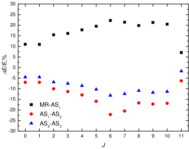
Figure 1: Convergence of the lowest states of the $4f^{11}5d$ configuration with $J=0-11$ in the energy spectrum (SD 4f strategy).

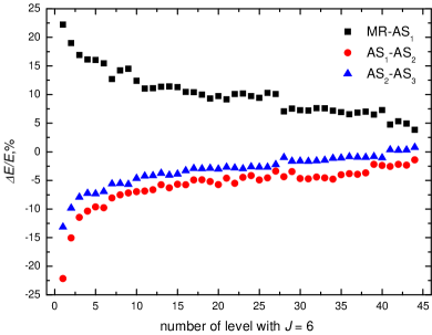
Figure 2: Convergence of all energy values of the $4f^{11}5d$ configuration with $J=6$ (SD 4f strategy).

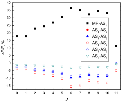
Figure 3: Convergence of the lowest states of $4f^{11}5d$ configuration with $J=0,11$ in the energy spectrum. Results are obtained using the SD 5d strategy (open symbols mark the results when the ZF^MCDHF approach at $AS_{2,3,4}$ is applied).

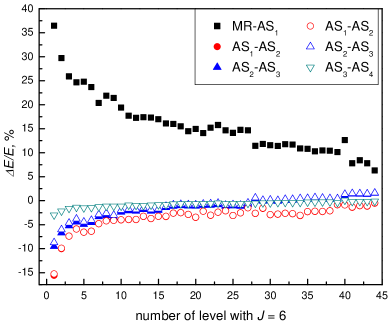
Figure 4: Convergence of all energy values of the $4f^{11}5d$ configuration with $J=6$. Results are obtained using the SD 5d strategy (open symbols mark the results when the ZF^MCDHF approach at $AS_{2,3,4}$ is applied).

The lowest levels according to Hund’s first rule have the largest multiplicity. For a given set of eigenstates, the lowest state will have largest multiplicity. Almost all the lowest levels for each $J$ in case of the $4f^{11}5d$ configuration have the largest multiplicity (except $J=9$), and all these levels converge slower than the higher ones (as it can be seen from Figures 2 and 4). However, even in the set of levels with the largest multiplicity, a large differences in convergence is observable (see Figures 1 and 3). From these Figures it can also be seen that the CSFs from the $AS_{1}$ (black squares) have the largest influence. The first active space has a larger influence on energy levels in the SD 5d strategy than in the SD 4f strategy.

The results of the SD 4f strategy substantially disagree with NIST/(SE) data (see Table 2) for states of the $4f^{11}5d$ configuration, and after adding one more layer ($AS_{3}$) to the computations, the disagreement increases. From the Table it is seen that after including substitutions from the $5d$ shell (SD 5d strategy) the results agree much better. The averaged uncertainty of obtained results from the SD 5d strategy at $AS_{2}$ is around 5.6% comparing with NIST or SE data. By studying the convergence of the results obtained using the SD 5d strategy we see similar trends as those from the SD 4f strategy. Firstly, energies for different $J$ values converge differently. Secondly, lower energy levels converge much slower than the higher energy levels. But in case of the SD 5d strategy the energies converge much faster comparing with the SD 4f strategy (see Figures 3 and 4). For example, the difference between $AS_{2}$ and $AS_{3}$ for $J=0$ is about 2.3% and 9.5% for lowest state with $J=6$.

4.2 Studies of core-valence and core-core electron correlations

The investigations of core-core and core-valence electron correlations contributions to the transition energies are presented in Table 3. From the Table it is seen that by including substitutions just from the valence shell ($4f$) and core shells ($5p$) or ($5s$) (SD 5p or SD 5s strategy) the results are in worse agreement with NIST/(SE). In case of the SD 5p strategy this disagreement is very large. The relative difference compared with NIST/(SE) data is reduced when substitutions from $4f$, $5d$ and $5p$ or $5s$ shells are allowed. The averaged uncertainty of the obtained results from strategies SrD 5p 5d, SD 5s 5d, SrD 5s 5p 5d, SD 5s 5p 5d is similar, around 5-7% comparing with NIST or SE data. As was mentioned above, inclusion of the substitutions from the core shells ($5p$ or $5s$) increases the number of CSFs dramatically (see Table 1). So for further investigations substitutions from the $5p$ and $5s$ shells were neglected.

4.3 Optimal strategy for electron correlations

The SD 5d strategy was chosen as the optimal strategy considering achieved accuracy of the results and the computational resources needed for the calculations. The main goal of this work is to obtain accurate energy levels of the ground and first excited configurations of Er²⁺. So we give priority to balanced electron correlation effects which improves the energy separations.

4.4 Impact of the zero-first-order method

The ZF method was applied at different stages of the calculations to reduce computation resources, as it was described in Section 3.4. The impact of the ZF method was studied using the SD 4f and SD 5d strategies. In the investigations of the effect of ZF on the energy levels all 399 states were included. The zero-first-order method (see SD 4f ZF^MCDHF column in Table 4) has up to 0.08% impact on the values of the energy levels at $AS_{3}$ if all levels are compared. From Table 5 we see that the ZF method for MCDHF calculations (see SD 5d ZF^MCDHF column) affects on average the values of the energy levels at $AS_{3}$ by 0.29%, and in some cases up to 1.01% .

The application of the ZF method for the RCI computation only (see SD 4f ZF_RCI column in Table 4), has a larger influence on the energy levels; it is up to 2.84% at $AS_{3}$ and 1.61% in average for all states. Using the SD 5d ZF_RCI strategy (see Table 5) the contribution of ZF in RCI is up to 2.69% at $AS_{3}$ and 1.45% in average for all states.

When the ZF method was applied for the RCI computations using orbitals from SD 4f ZF^MCDHF the energies changed in average about 0.5% (SD 4f ZF${}^{MCDHF}_{RCI}$) and up to 2.39% for some levels. Using the SD 5d ZF${}^{MCDHF}_{RCI}$ strategy (see Table 5) the influence of the ZF method is up to 3.95% at $AS_{3}$ and 0.66% in average for all states.

From the above study we infer that the impact of the ZF order method on the energy levels is very small in self consistent field computations for both strategies. In the case of the SD 5d ZF^MCDHF strategy, the effect on the energy levels at $AS_{3}$ is only 0.29%.

Table 4: Energy Levels from RCI Calculations Using the ZF Approach in Different Steps of the Calculations (SD 4f Strategy).

$LS$	POS	JP	NIST/(SE)	SD 4f			SD 4f ZFMCDHF			SD 4f ZFRCI			SD 4f ZF${}^{MCDHF}_{RCI}$
				$AS_{2}$	$AS_{3}$		$AS_{2}$	$AS_{3}$		$AS_{2}$	$AS_{3}$		$AS_{2}$	$AS_{3}$	$AS_{4}$
$4f^{12}~{}{}^{3}H$	1	6+	0.00	0	0		0	0.00		0	0		0	0	0
$4f^{12}~{}{}^{3}F$	1	4+	5081.79	5894	5744		5895	5744		5834	5628		5832	5617	5572
$4f^{12}~{}{}^{3}H$	1	5+	6969.78	6784	6805		6786	6806		6790	6791		6794	6796	6798
$4f^{12}~{}{}^{3}H$	2	4+	10785.48	10957	10889		10961	10889		10912	10786		10915	10785	10766
$4f^{12}~{}{}^{3}F$	1	3+	(12472.55)	13565	13282		13570	13279		13472	13076		13475	13066	13019
$4f^{12}~{}{}^{3}F$	1	2+	(13219.80)	14824	14446		14829	14442		14777	14290		14780	14280	14216
$4f^{12}~{}{}^{1}G$	3	4+	(18383.59)	18359	18381		18361	18388		18188	18116		18187	18108	18053
$4f^{11}~{}{}(^{4}I^{1})~{}{}5d~{}{}^{5}G$	1	6-	16976.09	18983	21480		18976	21466		19666	20919		19634	22004	23585
$4f^{11}~{}{}(^{4}I^{1})~{}{}5d~{}{}^{5}H$	1	7-	17647.76	19877	22337		19875	22323		20543	21751		20513	22839	24421
$4f^{11}~{}{}(^{4}I^{1})~{}{}5d~{}{}^{3}L$	1	9-	18976.74	20916	23382		20933	23369		21593	22753		21577	23859	25438
$4f^{11}~{}{}(^{4}I^{1})~{}{}5d~{}{}^{5}I$	1	8-	19918.17	22273	24699		22285	24685		22923	24060		21577	25163	26746
$4f^{11}~{}{}(^{4}I^{1})~{}{}5d~{}{}^{5}L$	1	10-	20470.13	21673	24130		21692	24116		22306	23463		22293	24575	26146
$4f^{11}~{}{}(^{4}I^{1})~{}{}5d~{}{}^{5}K$	2	9-	21688.17	23664	26085		23687	26071		24285	25387		24275	26504	28084
$4f^{11}~{}{}(^{4}I^{1})~{}{}5d~{}{}^{5}G$	1	5-	22016.77	24164	26648		24167	26634		24936	26172		24906	27264	28844
$4f^{11}~{}{}(^{4}I^{1})~{}{}5d~{}{}^{5}H$	2	6-	22606.07	24963	27418		24970	27404		25701	26896		25675	27993	29572
$4f^{11}~{}{}(^{4}I^{1})~{}{}5d~{}{}^{5}I$	2	8-	22951.42	25085	27514		25111	27501		25736	26835		25726	27954	29535
$4f^{11}~{}{}(^{4}I^{1})~{}{}5d~{}{}^{5}I$	2	7-	23302.78	26039	28459		26061	28445		26723	27834		26710	28948	30529
$4f^{11}~{}{}(^{4}I^{1})~{}{}5d~{}{}^{5}L$	3	8-	25482.12	27453	29916		27481	29903		28211	29364		28198	30479	32061
$4f^{11}~{}{}(^{4}I^{1})~{}{}5d~{}{}^{5}H$	3	5-	26192.66	29109	31551		29122	31537		29877	31044		29853	32145	33715
$4f^{11}~{}{}(^{4}I^{1})~{}{}5d~{}{}^{5}K$	3	7-	26579.91	29220	31644		29245	31630		29967	31094		29952	32206	33781
	1	4-	(26648.59)	28786	31252		28792	31238		29595	30816		29565	31908	33482
	2	4-	(29469.40)	32112	34506		32121	34492		32857	33980		32830	35074	36623
	3	4-	(30750.22)	34590	36669		34584	36655		35182	35938		35153	37015	38514
	4	4-	(32196.96)	35818	38077		35831	38064		36504	37462		36482	38560	40091
	5	4-	(33033.10)	36800	38990		36816	38976		37462	38323		37445	39432	40969
	6	4-	(35903.96)	40430	42276		40430	42262		41007	41478		40981	42564	44050
	7	4-	(37608.12)	41896	44068		41919	44054		42533	43359		42519	44467	45981
	8	4-	(39667.36)	43809	45645		43809	45631		44370	44833		44343	45916	47388
	9	4-	(40580.40)	44448	46293		44452	46279		44964	45424		44942	46513	48012
	10	4-	(46937.23)	44848	46678		44856	46664		45435	45881		45412	46975	48464
	3	9-	(27471.61)	28932	31400		28964	31386		29672	30820		29663	31942	33516
	3	6-	(27472.46)	30355	34985		30374	32747		31102	32230		31083	33335	34907
	4	6-	(28777.74)	32618	35063		32642	34972		33310	34342		33300	35463	37023
	5	6-	(30283.09)	32668	36114		32697	35049		33393	34505		33378	35614	37176
	6	6-	(31095.82)	33767	36114		33789	36100		34471	35516		34455	36623	38172
	7	6-	(33191.53)	36889	38955		36909	38941		37476	38145		37462	39243	40744
	8	6-	(33875.19)	38090	40207		38115	40194		38707	39459		38698	40581	42120
	9	6-	(35856.62)	39697	41952		39734	41939		40377	41260		40371	42385	43931
	10	6-	(36570.10)	40776	42673		40787	42659		41303	41822		41287	42926	44426
	3	5-	(27870.83)	31235	33646		31267	33632		31956	33014		31948	34138	35701
	4	5-	(29995.62)	33042	35388		33056	35374		33750	34811		33728	35909	37455
	5	5-	(31214.52)	34758	36967		34768	36954		35395	36273		35374	37363	38877
	6	5-	(32614.37)	35994	38025		35995	38011		36569	37289		36545	38380	39889
	7	5-	(33704.29)	37449	39616		37468	39602		38095	38931		38079	40039	41571
	8	5-	(36330.81)	40031	42203		40054	42189		40688	41505		40673	42564	44138
	9	5-	(36655.60)	41618	43638		41638	43624		42201	42850		42189	43961	45469
	10	5-	(39265.81)	44536	46335		44546	46321		45111	45507		45091	46601	48083
	11	5-	(40857.10)	45058	46878		45063	46864		45575	46024		45554	47116	48588
	12	5-	(46552.18)	45507	47406		45521	47393		46086	46602		46068	47703	49195
	13	5-	(48747.15)	47313	49233		47330	49219		47881	48424		47865	49525	51002
	4	8-	(28555.40)	30680	33109		30715	33095		31424	32525		31416	33650	35232
	5	8-	(31701.46)	33681	36102		33717	36089		34407	35485		34399	36609	38170
	4	7-	(28818.44)	31327	33744		31356	33731		32067	33172		32055	34289	35862
	5	7-	(29610.99)	31953	34373		31987	34359		32699	33791		32689	34913	36491
	6	7-	(32559.55)	35372	37743		35412	37729		36082	37093		36078	38221	39782
	7	7-	(36636.87)	36973	39291		37007	39277		37649	38597		37642	39716	41249
	1	3-	(29466.42)	31943	34353		31949	34339		32712	33871		32682	34961	36516
	2	3-	(31846.16)	34404	36802		34415	36788		35149	36282		35123	37379	38932
	3	3-	(33185.64)	37798	39691		37788	39677		38350	38906		38320	39982	41475
	4	3-	(36167.30)	40736	42934		40763	42920		41406	42218		41394	43330	44849
	5	3-	(37812.87)	42093	43938		42085	43923		42655	43141		42622	44215	45696
	6	3-	(38924.30)	42968	44779		42969	44765		43507	43943		43484	45031	46529
	7	3-	(40407.72)	44318	46177		44324	46163		44847	45302		44827	46395	47874
	1	2-	(38563.97)	34941	37339		34952	37325		35680	36810		35654	37907	39458

Table 5: Energy Levels from RCI Calculations Using the ZF Approach in Different Steps of the Calculations (SD 5d Strategy).

$LS$	POS	JP	NIST/(SE)	SD 5d			SD 5d ZFMCDHF			SD 5d ZFRCI			SD 5d ZF${}^{MCDHF}_{RCI}$
				$AS_{2}$	$AS_{3}$		$AS_{2}$	$AS_{3}$		$AS_{2}$	$AS_{3}$		$AS_{2}$	$AS_{3}$
$4f^{12}~{}{}^{3}H$	1	6+	0.00	0	0		0	0		0	0		0	0
$4f^{12}~{}{}^{3}F$	1	4+	5081.79	5895	5744		5895	5744		5833	5628		5832	5617
$4f^{12}~{}{}^{3}H$	1	5+	6969.78	6784	6805		6786	6806		6790	6791		6794	6796
$4f^{12}~{}{}^{3}H$	2	4+	10785.48	10958	10889		10961	10890		10912	10786		10916	10786
$4f^{12}~{}{}^{3}F$	1	3+	(12472.55)	13566	13282		13570	13279		13471	13075		13475	13066
$4f^{12}~{}{}^{3}F$	1	2+	(13219.80)	14825	14446		14829	14442		14776	14290		14781	14280
$4f^{12}~{}{}^{1}G$	3	4+	(18383.59)	18360	18381		18361	18388		18187	15728		18188	18109
$4f^{11}~{}{}(^{4}I^{1})~{}{}5d~{}{}^{5}G$	1	6-	16976.09	14673	16073		14638	15912		15109	15728		15045	16734
$4f^{11}~{}{}(^{4}I^{1})~{}{}5d~{}{}^{5}H$	1	7-	17647.76	15613	17006		15583	16849		16057	16642		15997	17652
$4f^{11}~{}{}(^{4}I^{1})~{}{}5d~{}{}^{3}L$	1	9-	18976.74	16725	18204		16721	18057		17194	17734		17150	18766
$4f^{11}~{}{}(^{4}I^{1})~{}{}5d~{}{}^{5}I$	1	8-	19918.17	17988	19380		17977	19226		18417	18924		18369	19951
$4f^{11}~{}{}(^{4}I^{1})~{}{}5d~{}{}^{5}L$	1	10-	20470.13	17644	19158		17640	19019		18088	18656		18048	19695
$4f^{11}~{}{}(^{4}I^{1})~{}{}5d~{}{}^{5}K$	2	9-	21688.17	19561	21006		19562	20861		19985	20485		19947	21528
$4f^{11}~{}{}(^{4}I^{1})~{}{}5d~{}{}^{5}G$	1	5-	22016.77	19890	21285		19866	21125		20456	21058		20396	22074
$4f^{11}~{}{}(^{4}I^{1})~{}{}5d~{}{}^{5}H$	2	6-	22606.07	20716	22102		20696	21944		21256	21822		21199	22842
$4f^{11}~{}{}(^{4}I^{1})~{}{}5d~{}{}^{5}I$	2	8-	22951.42	20903	22321		20906	22170		21357	21837		21318	22881
$4f^{11}~{}{}(^{4}I^{1})~{}{}5d~{}{}^{5}I$	2	7-	23302.78	21733	23103		21733	22946		22215	22689		22172	23727
$4f^{11}~{}{}(^{4}I^{1})~{}{}5d~{}{}^{5}L$	3	8-	25482.12	23276	24757		23283	24610		23839	24376		23797	25416
$4f^{11}~{}{}(^{4}I^{1})~{}{}5d~{}{}^{5}H$	3	5-	26192.66	24808	26162		24796	26001		25368	25881		25315	26907
$4f^{11}~{}{}(^{4}I^{1})~{}{}5d~{}{}^{5}K$	3	7-	26579.91	24959	26367		24963	26215		25510	26005		25467	27043
	1	4-	(26648.59)	24556	25947		24533	25789		25166	25762		25104	26776
	2	4-	(29469.40)	27877	29198		27858	29040		28423	28910		28365	29926
	3	4-	(30750.22)	30274	31299		30242	31141		30648	30782		30588	31783
	4	4-	(32196.96)	31408	32609		31401	32446		31894	32225		31845	33250
	5	4-	(33033.10)	32374	33454		32361	33291		32814	33018		32764	34044
	6	4-	(35903.96)	36133	36946		36106	36791		36501	36350		36444	37359
	7	4-	(37608.12)	37438	38533		37440	38367		37872	38055		37829	39088
	8	4-	(39667.36)	39556	40364		39530	40209		39911	39765		39854	40770
	9	4-	(40580.40)	40165	41000		40145	40846		40463	40318		40412	41330
	10	4-	(46937.23)	40498	41266		40482	41108		40866	40650		40815	41666
	3	9-	(27471.61)	24896	26416		24906	26274		25453	26006		25416	27055
	3	6-	(27472.46)	26082	27443		26077	27287		26623	27115		26575	28144
	4	6-	(28777.74)	28112	29360		28123	29190		28598	28957		28561	30003
	5	6-	(30283.09)	28454	29857		28453	29708		29009	29507		28963	30539
	6	6-	(31095.82)	29549	30894		29548	30745		30058	30480		30013	31510
	7	6-	(33191.53)	32635	33718		32634	33567		33025	33092		32982	34114
	8	6-	(33875.19)	33618	34659		33620	34495		34014	34125		33976	35170
	9	6-	(35856.62)	35430	36666		35446	36512		35906	36165		35871	37218
	10	6-	(36570.10)	36480	37345		36467	37193		36781	36644		36736	37669
	3	5-	(27870.83)	26706	27992		26714	27823		27225	27635		27185	28678
	4	5-	(29995.62)	28760	30057		28749	29902		29261	29690		29210	30711
	5	5-	(31214.52)	30474	31638		30459	31484		30890	31115		30839	32127
	6	5-	(32614.37)	31714	32739		31692	32585		32095	32222		32041	33237
	7	5-	(33704.29)	33073	34182		33069	34022		33511	33715		33466	34747
	8	5-	(36330.81)	35735	36870		35735	36714		36193	36386		36149	37420
	9	5-	(36655.60)	37138	38054		37135	37888		37503	37468		37461	38502
	10	5-	(39265.81)	40220	41002		40208	40847		40562	40325		40514	41344
	11	5-	(40857.10)	40672	41476		40651	41317		40976	40841		40924	41852
	12	5-	(46552.18)	41210	42034		41200	41878		41583	41409		41536	42432
	13	5-	(48747.15)	42975	43871		42968	43715		43336	43270		43291	44295
	4	8-	(28555.40)	26563	28010		26576	27863		27113	27607		27076	28658
	5	8-	(31701.46)	29611	31074		29626	30931		30149	30624		30114	31675
	4	7-	(28818.44)	27034	28431		27041	28278		27583	28061		27542	29102
	5	7-	(29610.99)	27752	29159		27763	29008		28303	28778		28264	29825
	6	7-	(32559.55)	31168	32535		31186	32385		31672	32063		31639	33116
	7	7-	(36636.87)	32864	34212		32877	34067		33355	33689		33320	34734
	1	3-	(29466.42)	27718	29057		27694	28899		28290	28822		28228	29834
	2	3-	(31846.16)	30216	31554		30200	31397		30772	31282		30715	32303
	3	3-	(33185.64)	33433	34279		33397	34120		33758	33701		33697	34700
	4	3-	(36167.30)	36191	37278		36197	37110		36645	36799		36603	37835
	5	3-	(37812.87)	37805	38620		37771	38464		38168	38032		38105	39027
	6	3-	(38924.30)	38621	39395		38597	39238		38938	38743		38883	39753
	7	3-	(40407.72)	39948	40754		39930	40596		40253	40068		40203	41083
	1	2-	(38563.97)	30760	32092		30742	31935		31306	31815		31248	32835

4.5 Final results

Based on the analysis made in previous sections, the SD 5d strategy was chosen as the optimal strategy. Therefore this strategy with the orbitals taken from the ZF^MCDHF strategy was used to continue computations in $AS_{4}$ basis. The final results of the present work are displayed in Table 6 together with NIST and SE data. In first column of the Table we give identifications of energy levels in $LS$ or $JJ$ (see definition in Gaigalas (2020), Eq. (10) and (16)) coupling from our computations, in second column identifications of energy levels are from Wyart et al. (1997). Labels in $LS$ coupling agree with identification given in the NIST database. Labels in $JJ$ coupling are given only for the part of the energy spectra that is used for the comparison with the results of Wyart et al. The averaged uncertainty of the computed energy levels is 5.24%, 2.68%, respectively for states of the ground and excited configurations (see Table 6 SD 5d ZF^MCDHF strategy $AS_{4}$). Root-mean-square (rms) deviations of these results for states of the ground and excited configurations from the NIST/(SE) data are 649 cm^-1, and 1571 cm^-1, respectively. If the ZF method is used in both the MCDHF and RCI calculations (SD 5d ZF${}^{MCDHF}_{RCI}$ strategy) the obtained data are in worse agreement (moderately about 7%) with NIST or SE data.

Figure 5 displays the differences between the NIST/(SE) energies and final results of the present study. As it can be seen from Figure 5 and Table 6 (energy levels marked in gray color), there is a significant disagreement between states with the following identifications $J$=4 Pos=10, $J$=5 Pos 12, $J$=5 Pos=13, $J$=7 Pos=7, and $J$=2 Pos=1. Energy differences exceed 2000 cm^-1 for these five energy levels. It is highly probable that the obtained differences result from incorrect ordering and incomplete identification of energy levels presented by Wyart et al. (1997). Only for one level ($J$=7 Pos=7) from the five above mentioned levels Wyart et al. (1997) give identification in $JJ$ coupling, for the four others only configurations are given. The level is identified as ${}^{4}F_{9/2}~{}5d_{5/2}$ ($J$=7). We have transformed ASFs from $LS$ to $JJ$ coupling using the Coupling program developed by Gaigalas (2020). The level $J$=7 Pos=7 has the $4f^{11}(^{4}I_{9/2})~{}5d_{5/2}~{}(9/2,5/2)$ label in $JJ$ coupling which disagree with Wyart et al. By looking at levels which match the identification given by Wyart et al. we see that there is a fit for $J$=7 Pos=8 with identification $4f^{11}(^{4}F_{9/2})~{}5d_{5/2}~{}(9/2,5/2)$. If we replace computed energy levels marked in gray color in Table 6 by energy levels suggested in Table 7 (presented by open red circles in Figure 6), agreement with the NIST/(SE) data is much better. The change in the differences between the NIST/(SE) energies and our final results is shown by dashed arrows in Figure 5. The rms deviation for states of the excited configuration (when five of the computed energy levels are replaced) is now only 747 cm^-1. By comparing the labels of the levels for which Wyart et al. gives the full identification with our identification in $JJ$ coupling, the labels from both studies agree except for the levels (namely $J$=4 Pos=8, $J$=6 Pos 5, $J$=6 Pos=10, $J$=5 Pos=3, and $J$=3 Pos=1). Level $J$=4 Pos=8 in the present work has the $4f^{11}(^{4}F_{7/2})~{}5d_{5/2}~{}(7/2,5/2)$ idendification; $J$=6 Pos 5 – $4f^{11}(^{4}I_{9/2})~{}5d_{3/2}~{}(9/2,3/2)$; $J$=6 Pos=10 – $4f^{11}(^{4}F_{9/2})~{}5d_{5/2}~{}(9/2,5/2)$; $J$=5 Pos=3 – $4f^{11}(^{4}I_{15/2})~{}5d_{5/2}~{}(15/2,5/2)$; and $J$=3 Pos=1 – $4f^{11}(^{4}I_{11/2})~{}5d_{5/2}~{}(11/2,5/2)$. It was observed that the identification given in (Wyart et al., 1997) for level $J$=3 Pos=1 is incorrect. That level was assigned as ${}^{4}I_{11/2}~{}5d_{3/2}$ but such a label for $J$=3 is not consistent with the selection rules. The deeper analysis of uncertainties estimation is complicated because complete identification of energy levels was not given in the paper by Wyart et al. (1997).

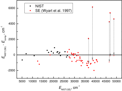
Figure 5: A comparison of energy levels between the NIST or SE values Wyart et al. (1997) and results of the present study. The dashed arrows indicate the improved agreement resulting from a re-identification of the levels in Wyart et al. (1997), see text for details.

Table 6: Comparison of Energy Levels from the Present Calculations Based on the SD 5d Strategy and Using the ZF Approach with NIST/SE data.

$LS$/$JJ$	label in Wyart et al. (1997)	POS	JP	NIST/(SE)	SD 5d ZFMCDHF			SD 5d ZF${}^{MCDHF}_{RCI}$
					$AS_{4}$			$AS_{4}$
$4f^{12}~{}{}^{3}H$		1	6+	0.00	0			0
$4f^{12}~{}{}^{3}F$		1	4+	5081.79	5731/	$-$12.77		5572 /	$-$9.65
$4f^{12}~{}{}^{3}H$		1	5+	6969.78	6814/	2.24		6798 /	2.47
$4f^{12}~{}{}^{3}H$		2	4+	10785.48	10890/	$-$0.97		10766/	0.18
$4f^{12}~{}{}^{3}F$		1	3+	(12472.55)	13267/	$-$6.37		13019/	$-$4.38
$4f^{12}~{}{}^{3}F$		1	2+	(13219.80)	14418/	$-$9.06		14216/	$-$7.54
$4f^{12}~{}{}^{1}G$		3	4+	(18383.59)	18393/	$-$0.05		18053/	1.80
$4f^{11}~{}{}(^{4}I^{1})~{}{}5d~{}{}^{5}G$		1	6-	16976.09	16391/	3.44		18186/	$-$7.13
$4f^{11}~{}{}(^{4}I^{1})~{}{}5d~{}{}^{5}H$		1	7-	17647.76	17333/	1.78		19110/	$-$8.29
$4f^{11}~{}{}(^{4}I^{1})~{}{}5d~{}{}^{3}L$		1	9-	18976.74	18524/	2.39		20211/	$-$6.51
$4f^{11}~{}{}(^{4}I^{1})~{}{}5d~{}{}^{5}I$		1	8-	19918.17	19672/	1.24		21401/	$-$7.44
$4f^{11}~{}{}(^{4}I^{1})~{}{}5d~{}{}^{5}L$		1	10-	20470.13	19537/	4.56		21155/	$-$3.34
$4f^{11}~{}{}(^{4}I^{1})~{}{}5d~{}{}^{5}K$		2	9-	21688.17	21342/	1.60		22986/	$-$5.98
$4f^{11}~{}{}(^{4}I^{1})~{}{}5d~{}{}^{5}G$		1	5-	22016.77	21604/	1.87		23527/	$-$6.86
$4f^{11}~{}{}(^{4}I^{1})~{}{}5d~{}{}^{5}H$		2	6-	22606.07	22421/	0.82		24297/	$-$7.48
$4f^{11}~{}{}(^{4}I^{1})~{}{}5d~{}{}^{5}I$		2	8-	22951.42	22629/	1.41		24329/	$-$6.00
$4f^{11}~{}{}(^{4}I^{1})~{}{}5d~{}{}^{5}I$		2	7-	23302.78	23392/	$-$0.38		25176/	$-$8.04
$4f^{11}~{}{}(^{4}I^{1})~{}{}5d~{}{}^{5}L$		3	8-	25482.12	25069/	1.62		26865/	$-$5.43
$4f^{11}~{}{}(^{4}I^{1})~{}{}5d~{}{}^{5}H$		3	5-	26192.66	26464/	$-$1.03		28349/	$-$8.23
$4f^{11}~{}{}(^{4}I^{1})~{}{}5d~{}{}^{5}K$		3	7-	26579.91	26661/	$-$0.31		28490/	$-$7.19
$4f^{11}~{}(^{4}I_{11/2})~{}5d_{3/2}~{}(11/2,3/2)$	${}^{4}I_{11/2}~{}5d_{3/2}$	1	4-	(26648.59)	26268/	1.43		28225/	$-$5.92
$4f^{11}~{}(^{4}I_{11/2})~{}5d_{5/2}~{}(11/2,5/2)$	$4f^{11}~{}5d$	2	4-	(29469.40)	29509/	$-$0.13		31348/	$-$6.37
$4f^{11}~{}(^{4}F_{9/2})~{}5d_{3/2}~{}(9/2,3/2)$	${}^{4}F_{9/2}~{}5d_{3/2}$	3	4-	(30750.22)	31599/	$-$2.76		33161/	$-$7.84
$4f^{11}~{}(^{4}I_{9/2})~{}5d_{3/2}~{}(9/2,3/2)$	$4f^{11}~{}5d$	4	4-	(32196.96)	32877/	$-$2.11		34655/	$-$7.63
$4f^{11}~{}(^{4}F_{9/2})~{}5d_{3/2}~{}(9/2,3/2)$	$4f^{11}~{}5d$	5	4-	(33033.10)	33728/	$-$2.10		35450/	$-$7.32
$4f^{11}~{}(^{4}F_{7/2})~{}5d_{3/2}~{}(7/2,3/2)$	${}^{4}F_{9/2}~{}5d$	6	4-	(35903.96)	37243/	$-$3.73		38722/	$-$7.85
$4f^{11}~{}(^{4}I_{9/2})~{}5d_{5/2}~{}(9/2,5/2)$	${}^{4}I_{9/2}~{}5d_{5/2}$	7	4-	(37608.12)	38774/	$-$3.10		40476/	$-$7.62
$4f^{11}~{}(^{4}F_{7/2})~{}5d_{5/2}~{}(7/2,5/2)$	${}^{4}F_{7/2}~{}5d_{3/2}$	8	4-	(39667.36)	40658/	$-$2.50		42126/	$-$6.20
$4f^{11}~{}(^{4}S_{3/2})~{}5d_{5/2}~{}(3/2,5/2)$	$4f^{11}~{}5d$	9	4-	(40580.40)	41258/	$-$1.67		42710/	$-$5.25
$4f^{11}~{}(^{4}F_{7/2})~{}5d_{3/2}~{}(7/2,3/2)$	$4f^{11}~{}5d$	10	4-	(46937.23)	41524/	11.53		43024/	8.34
$4f^{11}~{}(^{4}I_{13/2})~{}5d_{5/2}~{}(13/2,5/2)$	${}^{4}I_{13/2}~{}5d_{5/2}$	3	9-	(27471.61)	26769/	2.56		28508/	$-$3.77
$4f^{11}~{}(^{4}I_{13/2})~{}5d_{3/2}~{}(13/2,3/2)$	${}^{4}I_{13/2}~{}5d_{3/2}$	3	6-	(27472.46)	27729/	$-$0.93		29584/	$-$7.69
$4f^{11}~{}(^{4}I_{13/2})~{}5d_{5/2}~{}(13/2,5/2)$	${}^{4}I_{13/2}~{}5d_{5/2}$	4	6-	(28777.74)	29598/	$-$2.85		31434/	$-$9.23
$4f^{11}~{}(^{4}I_{9/2})~{}5d_{3/2}~{}(9/2,3/2)$	${}^{4}I_{11/2}~{}5d_{3/2}$	5	6-	(30283.09)	30162/	0.40		31975/	$-$5.59
$4f^{11}~{}(^{4}I_{9/2})~{}5d_{3/2}~{}(9/2,3/2)$	${}^{4}I_{9/2}~{}5d_{3/2}$	6	6-	(31095.82)	31189/	$-$0.30		32928/	$-$5.89
$4f^{11}~{}(^{4}I_{11/2})~{}5d_{5/2}~{}(11/2,5/2)$	$4f^{11}~{}5d$	7	6-	(33191.53)	34004/	$-$2.45		35490/	$-$6.93
$4f^{11}~{}(^{4}I_{11/2})~{}5d_{5/2}~{}(11/2,5/2)$	${}^{4}I_{11/2}~{}5d_{5/2}$	8	6-	(33875.19)	34893/	$-$3.01		36573/	$-$7.96
$4f^{11}~{}(^{4}I_{9/2}~{})5d_{5/2}~{}(9/2,5/2)$	$4f^{11}~{}5d$	9	6-	(35856.62)	36933/	$-$3.00		38635/	$-$7.75
$4f^{11}~{}(^{4}F_{9/2}~{})5d_{5/2}~{}(9/2,5/2)$	${}^{4}I_{9/2}~{}5d_{5/2}$	10	6-	(36570.10)	37627/	$-$2.89		39036/	$-$6.74
$4f^{11}~{}(^{4}I_{15/2})~{}5d_{5/2}~{}(15/2,5/2)$	${}^{4}I_{13/2}~{}5d_{5/2}$	3	5-	(27870.83)	28262/	$-$1.40		30113/	$-$8.04
$4f^{11}~{}(^{4}I_{11/2})~{}5d_{3/2}~{}(11/2,3/2)$	${}^{4}I_{11/2}~{}5d_{3/2}$	4	5-	(29995.62)	30345/	$-$1.16		32127/	$-$7.10
$4f^{11}~{}(^{4}I_{9/2})~{}5d_{3/2}~{}(9/2,3/2)$	$4f^{11}~{}5d$	5	5-	(31214.52)	31916/	$-$2.25		33507/	$-$7.34
$4f^{11}~{}(^{4}F_{9/2})~{}5d_{3/2}~{}(9/2,3/2)$	$4f^{11}~{}5d$	6	5-	(32614.37)	33040/	$-$1.31		34629/	$-$6.18
$4f^{11}~{}(^{4}F_{9/2})~{}5d_{3/2}~{}(9/2,3/2)$	$4f^{11}~{}5d$	7	5-	(33704.29)	34444/	$-$2.20		36152/	$-$7.26
$4f^{11}~{}(^{4}I_{9/2})~{}5d_{5/2}~{}(9/2,5/2)$	$4f^{11}~{}5d$	8	5-	(36330.81)	37154/	$-$2.27		38817/	$-$6.84
$4f^{11}~{}(^{4}F_{9/2})~{}5d_{5/2}~{}(9/2,5/2)$	$4f^{11}~{}5d$	9	5-	(36655.60)	38287/	$-$4.45		39879/	$-$8.79
$4f^{11}~{}(^{4}F_{7/2})~{}5d_{3/2}~{}(7/2,3/2)$	$4f^{11}~{}5d$	10	5-	(39265.81)	41260/	$-$5.08		42696/	$-$8.74
$4f^{11}~{}(^{2}H^{2}_{11/2})~{}5d_{3/2}~{}(11/2,3/2)$	$4f^{11}~{}5d$	11	5-	(40857.10)	41726/	$-$2.13		43204/	$-$5.75
$4f^{11}~{}(^{4}F_{7/2})~{}5d_{5/2}~{}(7/2,5/2)$	$4f^{11}~{}5d$	12	5-	(46552.18)	42297/	9.14		43795/	5.92
$4f^{11}~{}(^{2}H^{2}_{11/2})~{}5d_{5/2}~{}(11/2,5/2)$	$4f^{11}~{}5d$	13	5-	(48747.15)	44128/	9.48		45642/	6.37
$4f^{11}~{}(^{4}I_{13/2})~{}5d_{5/2}~{}(13/2,5/2)$	${}^{4}I_{13/2}~{}5d_{5/2}$	4	8-	(28555.40)	28325/	0.81		30112/	$-$5.45
$4f^{11}~{}(^{4}I_{11/2})~{}5d_{5/2}~{}(11/2,5/2)$	${}^{4}I_{11/2}~{}5d_{5/2}$	5	8-	(31701.46)	31400/	0.95		33108/	$-$4.44
$4f^{11}~{}(^{4}I_{11/2})~{}5d_{3/2}~{}(11/2,3/2)$	${}^{4}I_{11/2}~{}5d_{3/2}$	4	7-	(28818.44)	28722/	0.33		30546/	$-$5.99
$4f^{11}~{}(^{4}I_{13/2})~{}5d_{5/2}~{}(13/2,5/2)$	${}^{4}I_{13/2}~{}5d_{5/2}$	5	7-	(29610.99)	29454/	0.53		31269/	$-$5.60
$4f^{11}~{}(^{4}I_{11/2})~{}5d_{5/2}~{}(11/2,5/2)$	${}^{4}I_{11/2}~{}5d_{5/2}$	6	7-	(32559.55)	32825/	$-$0.82		34542/	$-$6.09
$4f^{11}~{}(^{4}I_{9/2})~{}5d_{5/2}~{}(9/2,5/2)$	${}^{4}F_{9/2}~{}5d_{5/2}$	7	7-	(36636.87)	34516/	5.79		36135/	1.37
$4f^{11}~{}(^{4}I_{11/2})~{}5d_{5/2}~{}(11/2,5/2)$	${}^{4}I_{11/2}~{}5d_{3/2}$	1	3-	(29466.42)	29374/	0.31		31265/	$-$6.10
$4f^{11}~{}(^{4}I_{9/2})~{}5d_{5/2}~{}(9/2,5/2)$	${}^{4}I_{9/2}~{}5d_{5/2}$	2	3-	(31846.16)	31869/	$-$0.07		33733/	$-$5.92
$4f^{11}~{}(^{4}F_{9/2})~{}5d_{3/2}~{}(9/2,3/2)$	${}^{4}F_{9/2}~{}5d_{3/2}$	3	3-	(33185.64)	34565/	$-$4.16		36072/	$-$8.70
$4f^{11}~{}(^{4}I_{9/2})~{}5d_{3/2}~{}(9/2,3/2)$	$4f^{11}~{}5d$	4	3-	(36167.30)	37527/	$-$3.76		39226/	$-$8.46
$4f^{11}~{}(^{4}F_{7/2})~{}5d_{3/2}~{}(7/2,3/2)$	$4f^{11}~{}5d$	5	3-	(37812.87)	38909/	$-$2.90		40386/	$-$6.81
$4f^{11}~{}(^{4}F_{7/2})~{}5d_{3/2}~{}(7/2,3/2)$	$4f^{11}~{}5d$	6	3-	(38924.30)	39652/	$-$1.87		41122/	$-$5.65
$4f^{11}~{}(^{4}F_{9/2})~{}5d_{5/2}~{}(9/2,5/2)$	$4f^{11}~{}5d$	7	3-	(40407.72)	41020/	$-$1.51		41122/	$-$5.01
$4f^{11}~{}(^{4}I_{9/2})~{}5d_{5/2}~{}(9/2,5/2)$	$4f^{11}~{}5d$	1	2-	(38563.97)	32408/	15.96		34263/	11.15

Note. — The relative difference compared with NIST/(SE) data is given in percent.

Table 7: The Proposed Energy Levels in Comparison with NIST/(SE) Data and Their Relative Difference (Given in Percent).

JP	NIST/(SE)	iden. in Wyart et al. (1997)	POS			SD 5d ZFMCDHF ($AS_{4}$)					iden. in present work
4-	(46937.23)		10	$\rightarrow$	15	41524/	11.53	$\rightarrow$	47046/	$-$0.23
5-	(46552.18)		12	$\rightarrow$	16	42297/	9.14	$\rightarrow$	47467/	$-$1.96
5-	(48747.15)		13	$\rightarrow$	17	44128/	9.48	$\rightarrow$	48836/	$-$0.18
7-	(36636.87)	${}^{4}F_{9/2}~{}5d_{5/2}$	7	$\rightarrow$	8	34516/	5.79	$\rightarrow$	37645/	$-$2.75	$4f^{11}(^{4}F_{9/2})~{}5d_{5/2}~{}(9/2,5/2)$
2-	(38563.97)		1	$\rightarrow$	3	32408/	15.96	$\rightarrow$	39173/	$-$1.58

The full energy spectrum (energy levels for 399 states) with unique labels and with atomic state function composition in $LS$ coupling using the SD 5d ZF^MCDHF strategy is presented in machine-readable format in Table 8.

Table 8: Energy Levels (in cm^-1) and Atomic State Function Composition of the Ground [Xe]$4f^{12}$ and First Excited [Xe]$4f^{11}5d$ Configurations for the Er²⁺ ion.

No.	POS	$J$	P	$E$	label	comp.
1	1	6	+	0.00	$4f^{12}~{}^{3}H$	0.95
2	1	4	+	5730.98	$4f^{12}~{}^{3}F$	0.56 + 0.29 $4f^{12}~{}^{1}G$ + 0.11 $4f^{12}~{}^{3}H$
3	1	5	+	6813.74	$4f^{12}~{}^{3}H$	0.95
4	2	4	+	10889.64	$4f^{12}~{}^{3}H$	0.59 + 0.29 $4f^{12}~{}^{3}F$ + 0.07 $4f^{12}~{}^{1}G$
5	1	3	+	13267.28	$4f^{12}~{}^{3}F$	0.95
6	1	2	+	14417.89	$4f^{12}~{}^{3}F$	0.81 + 0.13 $4f^{12}~{}^{1}D$
7	1	6	$-$	16391.49	$4f^{11}~{}(^{4}I^{1})~{}5d~{}^{5}G$	0.75 + 0.13 $4f^{11}~{}(^{4}I^{1})~{}5d~{}^{5}H$ + 0.02 $4f^{11}~{}(^{2}K^{1})~{}5d~{}^{3}H$
8	1	7	$-$	17333.10	$4f^{11}~{}(^{4}I^{1})~{}5d~{}^{5}H$	0.76 + 0.11 $4f^{11}~{}(^{4}I^{1})~{}5d~{}^{5}I$ + 0.02 $4f^{11}~{}(^{4}G^{1})~{}5d~{}^{5}H$
9	3	4	+	18392.93	$4f^{12}~{}^{1}G$	0.59 + 0.25 $4f^{12}~{}^{3}H$ + 0.11 $4f^{12}~{}^{3}F$
10	1	9	$-$	18523.58	$4f^{11}~{}(^{4}I^{1})~{}5d~{}^{3}L$	0.43 + 0.33 $4f^{11}~{}(^{4}I^{1})~{}5d~{}^{5}L$ + 0.17 $4f^{11}~{}(^{4}I^{1})~{}5d~{}^{5}K$
11	1	10	$-$	19537.18	$4f^{11}~{}(^{4}I^{1})~{}5d~{}^{5}L$	0.92 + 0.02 $4f^{11}~{}(^{2}K^{1})~{}5d~{}^{3}M$
12	1	8	$-$	19671.88	$4f^{11}~{}(^{4}I^{1})~{}5d~{}^{5}I$	0.44 + 0.28 $4f^{11}~{}(^{4}I^{1})~{}5d~{}^{5}K$ + 0.15 $4f^{11}~{}(^{4}I^{1})~{}5d~{}^{3}K$
13	2	9	$-$	21341.61	$4f^{11}~{}(^{4}I^{1})~{}5d~{}^{5}K$	0.71 + 0.21 $4f^{11}~{}(^{4}I^{1})~{}5d~{}^{3}L$
14	1	5	$-$	21604.17	$4f^{11}~{}(^{4}I^{1})~{}5d~{}^{5}G$	0.65 + 0.17 $4f^{11}~{}(^{4}I^{1})~{}5d~{}^{5}H$ + 0.05 $4f^{11}~{}(^{4}I^{1})~{}5d~{}^{3}G$
15	2	6	$-$	22420.54	$4f^{11}~{}(^{4}I^{1})~{}5d~{}^{5}H$	0.54 + 0.16 $4f^{11}~{}(^{4}I^{1})~{}5d~{}^{5}G$ + 0.11 $4f^{11}~{}(^{4}I^{1})~{}5d~{}^{5}I$
16	2	8	$-$	22628.77	$4f^{11}~{}(^{4}I^{1})~{}5d~{}^{3}K$	0.29 + 0.40 $4f^{11}~{}(^{4}I^{1})~{}5d~{}^{5}I$ + 0.09 $4f^{11}~{}(^{4}I^{1})~{}5d~{}^{5}L$
17	2	7	$-$	23392.31	$4f^{11}~{}(^{4}I^{1})~{}5d~{}^{3}I$	0.23 + 0.31 $4f^{11}~{}(^{4}I^{1})~{}5d~{}^{5}I$ + 0.17 $4f^{11}~{}(^{4}I^{1})~{}5d~{}^{5}K$
18	3	8	$-$	25069.42	$4f^{11}~{}(^{4}I^{1})~{}5d~{}^{5}L$	0.49 + 0.25 $4f^{11}~{}(^{4}I^{1})~{}5d~{}^{3}K$ + 0.20 $4f^{11}~{}(^{4}I^{1})~{}5d~{}^{3}L$
19	1	4	$-$	26268.28	$4f^{11}~{}(^{4}I^{1})~{}5d~{}^{5}G$	0.59 + 0.25 $4f^{11}~{}(^{4}I^{1})~{}5d~{}^{5}H$ + 0.03 $4f^{11}~{}(^{2}H^{2})~{}5d~{}^{3}F$
20	2	5	$-$	26463.59	$4f^{11}~{}(^{4}I^{1})~{}5d~{}^{5}H$	0.45 + 0.24 $4f^{11}~{}(^{4}I^{1})~{}5d~{}^{3}G$ + 0.09 $4f^{11}~{}(^{4}I^{1})~{}5d~{}^{5}I$

Note. — Table 8 is published in its entirety in the machine-readable format. Part of the values are shown here for guidance regarding its form and content.

5 Transition data results

The wave functions from the SD 5d and SD 5d ZF^MCDHF strategies, which were chosen as the optimal computational schemes, were used to compute E1 transition data between states of the [Xe]$4f^{12}$ and [Xe]$4f^{11}5d$ configurations. The accuracy of the transition data obtained in this work was evaluated by:

1. calculating parameter $dT$, which shows the disagreement between the length and velocity forms of the computed transition rates;

2. analyzing the convergence of the computed transition rates in the length and velocity forms;

3. analyzing the dependence of the transition rate on the gauge parameter $G$;

4. analyzing the dependence of cancellation factor on the gauge parameter $G$;

5. comparing computed transition data with other experimental or theoretical calculations.

For these investigations a few strong transitions have been chosen as examples. The evaluation of transition data will be presented in the sections below.

Computed transition data, such as wavelengths, weighted oscillator strengths, transition rates of E1 along with the accuracy indicator $dT$, are given in machine-readable format in Table 9.

5.1 Disagreement between the length and velocity and their convergence

In a variational approach the wave functions are optimized on an energy expression. In general this gives a better representation of the outer part of the wave functions, thus favoring the length form. The velocity form contains a dependence on the transition energy in the matrix element, which may affect the accuracy of the evaluation. Due to the above mentioned reasons, a much slower convergence of the velocity gauge is expected (Ynnerman & Fischer, 1995). However, a recent paper by Papoulia et al. (2019), analyzing in detail the convergence properties of transitions in light elements, suggests that transition probabilities in the Coulomb gauge may give the more accurate values. Thus, it is important to systematically study the transition data to see which gauge results in the most rapid convergence.

The convergence of the transition rates in both gauges with the increasing active spaces is presented in Figures 6 and 7. From these Figures it is seen that transition probabilities in the Babushkin gauge are more stable to electron correlation effects than the probabilities in the Coulomb gauge. The $dT$ for the analyzed transitions based on the final $AS_{4}$ in the SD 5d ZF^MCDHF strategy are 12% for $4f^{12}~{}{}^{3}P_{0}$ – $4f^{11}~{}{}(^{2}F^{1})~{}{}5d~{}{}^{3}P_{1}$, 23% for $4f^{12}~{}{}^{1}S_{0}$ – $4f^{11}~{}{}(^{2}F^{1})~{}{}5d~{}{}^{1}P_{1}$ (Figure 6); 3% for $4f^{12}~{}{}^{3}P_{2}$ – $4f^{11}~{}{}(^{2}F^{2})~{}{}5d~{}{}^{1}P_{1}$ and 5% for$4f^{12}~{}{}^{3}P_{2}$ – $4f^{11}~{}{}(^{2}F^{1})~{}{}5d~{}{}^{3}P_{1}$(Figure 7).

Analyzing the impact of the ZF method on the transition rates, we see that ZF^MCDHF $AS_{3}$ reduces transition rates compared to those from the SD 5d strategy. The transition rates in Coulomb gauge change even more than those in the Babushkin gauge. Transition rates in Babushkin gauge decreases just by a few percent for the analyzed transitions. The above analysis shows that the Babushkin gauge is the preferred one.

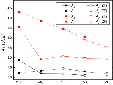
Figure 6: Convergence of E1 transition probabilities using the SD 5d strategy (open symbols mark the results when the ZF^MCDHF approach is applied). The $4f^{12}~{}{}^{3}P_{0}$ – $4f^{11}~{}{}(^{2}F^{1})~{}{}5d~{}{}^{3}P_{1}$ transition is marked in black and the $4f^{12}~{}{}^{1}S_{0}$ – $4f^{11}~{}{}(^{2}F^{1})~{}{}5d~{}{}^{1}P_{1}$ transition in red.

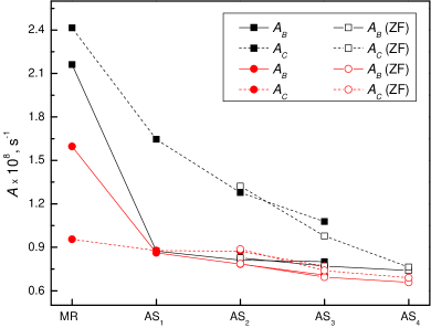
Figure 7: Convergence of E1 transition probabilities using the SD 5d strategy (open symbols mark the results when the ZF^MCDHF approach is applied). The $4f^{12}~{}{}^{3}P_{2}$ – $4f^{11}~{}{}(^{2}F^{2})~{}{}5d~{}{}^{1}P_{1}$ transition is marked in black and the $4f^{12}~{}{}^{3}P_{2}$ – $4f^{11}~{}{}(^{2}F^{1})~{}{}5d~{}{}^{3}P_{1}$ transition in red.

5.2 Gauge dependence

In Figures 8–11 the dependence of the transition probabilities for the different active space calculations on the gauge parameter $G$ is displayed. In each of these Figures the position of Coulomb and Babushkin gauges are marked by dotted lines. For some of analyzed transitions the curves of gauge dependence intersect at some point. The cross points are marked by dotted lines and the values are placed on the axis. The curves cross at around $G=1.7$ (very close to the Babushkin form) for the $4f^{12}~{}{}^{1}S_{0}$ – $4f^{11}~{}{}(^{2}F^{1})~{}{}5d~{}{}^{1}P_{1}$ (Figure 8) and $4f^{12}~{}{}^{3}P_{2}$ – $4f^{11}~{}{}(^{2}F^{1})~{}{}5d~{}{}^{1}P_{1}$ (Figure 10) transitions. For the $4f^{12}~{}{}^{3}P_{0}$ – $4f^{11}~{}{}(^{2}F^{1})~{}{}5d~{}{}^{3}P_{1}$ transition (Figure 9) the most of curves (except the curve of gauge dependence with $AS_{1}$) intersect at around $G=3.4$. In case of the $4f^{12}~{}{}^{3}P_{2}$ – $4f^{11}~{}{}(^{2}F^{1})~{}{}5d~{}{}^{3}P_{1}$ transition (Figure 11) the curves do not intersect at one point. From these Figures we can see that by increasing the active space, the curves of gauge dependence approach straight lines. At $AS_{4}$ (final results) these curves are very close to straight lines. It means that the wave functions should be quite accurate.

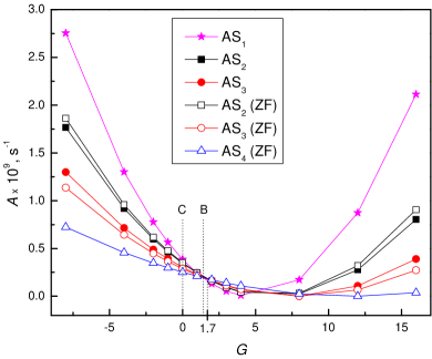
Figure 8: The gauge dependence of the $4f^{12}~{}{}^{1}S_{0}$ – $4f^{11}~{}{}(^{2}F^{1})~{}{}5d~{}{}^{1}P_{1}$ E1 transition probability for the different active space calculations using the SD 5d strategy (open symbols mark the results when the ZF^MCDHF approach is applied).

Figure 9: The gauge dependence of the $4f^{12}~{}{}^{3}P_{0}$ – $4f^{11}~{}{}(^{2}F^{1})~{}{}5d~{}{}^{3}P_{1}$ E1 transition probability for the different active space calculations using the SD 5d strategy (open symbols mark the results when the ZF^MCDHF approach is applied).

Figure 10: The gauge dependence of the $4f^{12}~{}{}^{3}P_{2}$ – $4f^{11}~{}{}(^{2}F^{2})~{}{}5d~{}{}^{1}P_{1}$ E1 transition probability for the different active space calculations using the SD 5d strategy (open symbols mark the results when the ZF^MCDHF approach is applied).

Figure 11: The gauge dependence of the $4f^{12}~{}{}^{3}P_{2}$ – $4f^{11}~{}{}(^{2}F^{1})~{}{}5d~{}{}^{3}P_{1}$ E1 transition probability for the different active space calculations using the SD 5d strategy (open symbols mark the results when the ZF^MCDHF approach is applied).

5.3 Cancellation factor

Figures 12 and 13 show the CF as a function of the increasing active space for the SD 5d strategy. From the Figures it is seen that CF in the Babushkin gauge for the analyzed transitions in all active spaces are lager than in the Coulomb gauge. In Figure 14 and 15 we present the dependence of CF on the gauge parameter $G$ using the SD 5d ZF^MCDHF strategy (at $AS_{4}$). The CF is presented for the four analyzed transitions. The CFs in Babushkin gauge for these transitions are much larger than 0.1 or 0.05, and in all cases they are the largest ones. They are even larger than at the cross points, where gauge dependence curves from different active spaces intersect. The CFs in Coulomb gauge for the transitions $4f^{12}~{}{}^{3}P_{2}$ – $4f^{11}~{}{}(^{2}F^{2})~{}{}5d~{}{}^{1}P_{1}$ and $4f^{12}~{}{}^{3}P_{2}$ – $4f^{11}~{}{}(^{2}F^{1})~{}{}5d~{}{}^{3}P_{1}$ (Figure 15) are smaller than 0.05, which means that in velocity form there is a strong cancellation effect. For the $4f^{12}~{}{}^{3}P_{0}$ – $4f^{11}~{}{}(^{2}F^{1})~{}{}5d~{}{}^{3}P_{1}$ and $4f^{12}~{}{}^{1}S_{0}$ – $4f^{11}~{}{}(^{2}F^{1})~{}{}5d~{}{}^{1}P_{1}$ (Figure 14) transitions, the CF in the Coulomb gauge is around 0.05. The analysis shows that transition data in the Babushkin gauge are less affected by cancellation effects than transition data in the velocity gauge.

Figure 12: Cancellation factor dependence on the active space. The $4f^{12}~{}{}^{3}P_{0}$ – $4f^{11}~{}{}(^{2}F^{1})~{}{}5d~{}{}^{3}P_{1}$ transition is marked in black and the $4f^{12}~{}{}^{1}S_{0}$ – $4f^{11}~{}{}(^{2}F^{1})~{}{}5d~{}{}^{1}P_{1}$ transition in red.

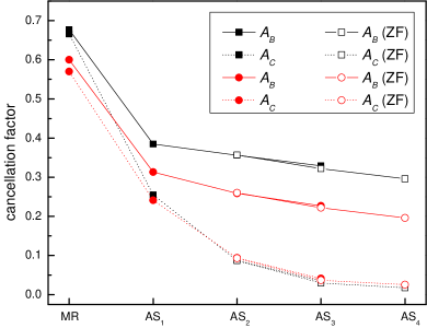
Figure 13: Cancellation factor dependence on the active space. The $4f^{12}~{}{}^{3}P_{2}$ – $4f^{11}~{}{}(^{2}F^{2})~{}{}5d~{}{}^{1}P_{1}$ transition is marked in black and the $4f^{12}~{}{}^{3}P_{2}$ – $4f^{11}~{}{}(^{2}F^{1})~{}{}5d~{}{}^{3}P_{1}$ transition in red.

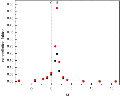
Figure 14: Cancellation factor dependence on gauge using the SD 5d ZF^MCDHF strategy (at $AS_{4}$). The $4f^{12}~{}{}^{3}P_{0}$ – $4f^{11}~{}{}(^{2}F^{1})~{}{}5d~{}{}^{3}P_{1}$ transition is marked and in black and the $4f^{12}~{}{}^{1}S_{0}$ – $4f^{11}~{}{}(^{2}F^{1})~{}{}5d~{}{}^{1}P_{1}$ transition is marked in red.

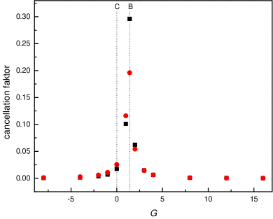
Figure 15: Cancellation factor dependence on gauge using the SD 5d ZF^MCDHF strategy (at $AS_{4}$). The $4f^{12}~{}{}^{3}P_{2}$ – $4f^{11}~{}{}(^{2}F^{2})~{}{}5d~{}{}^{1}P_{1}$ transition is marked and in black and the $4f^{12}~{}{}^{3}P_{2}$ – $4f^{11}~{}{}(^{2}F^{1})~{}{}5d~{}{}^{3}P_{1}$ transition is marked in red.

5.4 Comparison with other computations

No experimental transition rates for the studied configurations of Er²⁺ are available. The transition data obtained using the SD 5d ZF^MCDHF strategy (at $AS_{4}$) are compared with rates presented by Wyart et al. (1997) and Biémont et al. (2001). They used experimental transition wavelengths to compute transition data. Biémont et al. (2001) used the Cowan code and included core-polarization effects in the computations.

Figure 16 presents a comparison of obtained transition wavelengths with experimental data, which were presented in the paper by Wyart et al. (1997). The agreement between the computed wavelengths and the experimental ones is very good. Almost all compared lines achieve 5% uncertainty. In Figure 17 the comparison of transition rates (given in Babushkin gauge) of the present work with rates available from other computations (Wyart et al., 1997; Biémont et al., 2001) is displayed. It is seen that there is a good agreement with values from other authors for the stronger transitions. However, the transitions presented in the Figure are not the strongest obtained in this work. The strongest transition have rates of the order $10^{8}$ s^-1. By applying replacement in the energy levels discussed in Section 4.5 we achieve better agreement for wavelength and transition rate of marked transition (see open symbols in Figures 16 and 17).

Figure 16: Comparison of transition wavelengths between our computed data (comp.) using the SD 5d ZF^MCDHF strategy (at $AS_{4}$) and experimental data presented in the paper by Wyart et al. Wyart et al. (1997). The thick line corresponds to perfect agreement, while thin solid and dashed lines correspond to 5% and 10% deviations. The dashed arrows indicate the improved agreement by applying replacement in the energy levels discussed in Section 4.5.

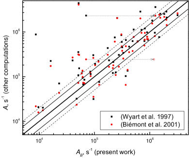
Figure 17: Comparison of transition rates of present work ($A$ is given in Babushkin gauge) with rates presented in Wyart et al. (1997) and Biémont et al. (2001). The data from Wyart et al. (1997) are marked by black squares and the red circles correspond to the results by Biémont et al. Biémont et al. (2001). The thick line corresponds to perfect agreement, while the thin solid and dashed lines correspond to deviations by factors of 1.5 and 2.0, respectively. The dashed arrows indicate the improved agreement by applying replacement in the energy levels discussed in Section 4.5.

Table 9: Transition Energies $\Delta E$ (in cm^-1), Transition Wavelengths $\lambda$ (in Å), Weighted Oscillator Strengths $gf$ and Transition Rates $A$ (in s^-1) for E1 Transitions of the Er²⁺ Ion.

No.(u)	$J_{u}$	Pu	state(u)	No.(l)	$J_{l}$	Pl	state(l)	$\Delta E$	$\lambda$	$A$	$gf$	$dT$
7	6	$-$	$4f^{11}~{}(^{4}I^{1})~{}5d~{}^{5}G$	1	6	+	$4f^{12}~{}^{3}H$	16391	6100.73	8.417E+02	6.106E$-$05	0.855
7	6	$-$	$4f^{11}~{}(^{4}I^{1})~{}5d~{}^{5}G$	3	5	+	$4f^{12}~{}^{3}H$	9577	10440.87	1.402E+01	2.978E$-$06	0.919
8	7	$-$	$4f^{11}~{}(^{4}I^{1})~{}5d~{}^{5}H$	1	6	+	$4f^{12}~{}^{3}H$	17333	5769.31	4.336E$-$01	3.246E$-$08	1.000
14	5	$-$	$4f^{11}~{}(^{4}I^{1})~{}5d~{}^{5}G$	1	6	+	$4f^{12}~{}^{3}H$	21604	4628.74	5.100E+04	1.802E$-$03	0.711
14	5	$-$	$4f^{11}~{}(^{4}I^{1})~{}5d~{}^{5}G$	2	4	+	$4f^{12}~{}^{3}F$	15873	6299.93	6.063E+04	3.968E$-$03	0.685
14	5	$-$	$4f^{11}~{}(^{4}I^{1})~{}5d~{}^{5}G$	3	5	+	$4f^{12}~{}^{3}H$	14790	6761.13	9.658E+03	7.280E$-$04	0.771
14	5	$-$	$4f^{11}~{}(^{4}I^{1})~{}5d~{}^{5}G$	4	4	+	$4f^{12}~{}^{3}H$	10714	9333.12	4.760E+03	6.837E$-$04	0.780
14	5	$-$	$4f^{11}~{}(^{4}I^{1})~{}5d~{}^{5}G$	9	4	+	$4f^{12}~{}^{1}G$	3211	31140.62	4.578E+01	7.321E$-$05	0.962
15	6	$-$	$4f^{11}~{}(^{4}I^{1})~{}5d~{}^{5}H$	1	6	+	$4f^{12}~{}^{3}H$	22420	4460.20	3.113E+05	1.207E$-$02	0.551
15	6	$-$	$4f^{11}~{}(^{4}I^{1})~{}5d~{}^{5}H$	3	5	+	$4f^{12}~{}^{3}H$	15606	6407.46	1.165E+04	9.318E$-$04	0.700
17	7	$-$	$4f^{11}~{}(^{4}I^{1})~{}5d~{}^{3}I$	1	6	+	$4f^{12}~{}^{3}H$	23392	4274.91	7.104E+05	2.920E$-$02	0.517
19	4	$-$	$4f^{11}~{}(^{4}I^{1})~{}5d~{}^{5}G$	2	4	+	$4f^{12}~{}^{3}F$	20537	4869.19	8.829E+02	2.824E$-$05	0.084
19	4	$-$	$4f^{11}~{}(^{4}I^{1})~{}5d~{}^{5}G$	3	5	+	$4f^{12}~{}^{3}H$	19454	5140.19	9.666E+03	3.446E$-$04	0.595
19	4	$-$	$4f^{11}~{}(^{4}I^{1})~{}5d~{}^{5}G$	4	4	+	$4f^{12}~{}^{3}H$	15378	6502.53	2.340E+03	1.335E$-$04	0.796
19	4	$-$	$4f^{11}~{}(^{4}I^{1})~{}5d~{}^{5}G$	5	3	+	$4f^{12}~{}^{3}F$	13001	7691.72	1.108E+04	8.847E$-$04	0.728
19	4	$-$	$4f^{11}~{}(^{4}I^{1})~{}5d~{}^{5}G$	9	4	+	$4f^{12}~{}^{1}G$	7875	12697.85	9.995E+01	2.174E$-$05	0.682
20	5	$-$	$4f^{11}~{}(^{4}I^{1})~{}5d~{}^{5}H$	1	6	+	$4f^{12}~{}^{3}H$	26463	3778.78	2.335E+05	5.499E$-$03	0.746
20	5	$-$	$4f^{11}~{}(^{4}I^{1})~{}5d~{}^{5}H$	2	4	+	$4f^{12}~{}^{3}F$	20732	4823.32	3.069E+05	1.177E$-$02	0.615
20	5	$-$	$4f^{11}~{}(^{4}I^{1})~{}5d~{}^{5}H$	3	5	+	$4f^{12}~{}^{3}H$	19649	5089.10	3.843E+01	1.641E$-$06	0.983
20	5	$-$	$4f^{11}~{}(^{4}I^{1})~{}5d~{}^{5}H$	4	4	+	$4f^{12}~{}^{3}H$	15573	6420.98	6.119E+04	4.160E$-$03	0.701

Note. — All transition data are in length form. $dT$ is the relative difference of the transition rates in length and velocity form as given by equation 10. Table 9 is published in its entirety in the machine-readable format. Part of the values are shown here for guidance regarding its form and content.

6 Summary and conclusion

In the present paper energy levels of the ground [Xe]$4f^{12}$ and first excited [Xe]$4f^{11}5d$ configurations for Er²⁺ ion were computed using the GRASP2018 package. Transition data for E1 transitions between computed states are presented. The accuracy of the obtained results is evaluated.

From the studies of the Er²⁺ ion, and also from the previous investigations of Nd ions, it was observed that in such calculations to get the correct order of ground and excited configurations it is important to freeze the wave functions of ground configuration.

The valence-valence, core-valence, and core-core electron correlations were studied using different strategies. This analysis has led to the final results in which the main balance electron correlation effects (mainly from VV substitutions) were included. This allows us to improve accuracy of the energy difference between different configurations considering the computational resources needed for the computations of such a complex system.

The rms deviations of the final results (using SD 5d ZF^MCDHF strategy) from the NIST or SE data for states of the ground and excited configurations are 649 cm^-1, and 747 cm^-1, respectively.

Having analyzed convergence trends and dependencies of the gauge parameter $G$, we propose, for the Er²⁺ ion, to use transition rates in the Babushkin gauge.

There is a lack of atomic data for the lanthanides. The present study is a first step towards the goal to provide this data with an accuracy high enough for opacity modeling.

References

- Biémont et al. (2001) Biémont, E., Garnir, H. P., Bastin, T., et al. 2001, Mon. Not. R. Astron. Soc., 321, 481
- Cowan (1981) Cowan, R. 1981, The Theory of Atomic Structure and Spectra (University of California Press, Berkeley, CA)
- Cowley & Crosswhite (1978) Cowley, C. R., & Crosswhite, H. M. 1978, PASP, 90, 108
- Cowley & Greenberg (1987) Cowley, C. R., & Greenberg, M. 1987, PASP, 99, 1201
- Cowley & Mathys (1998) Cowley, C. R., & Mathys, G. 1998, A&A, 339, 165
- Dyall et al. (1989) Dyall, K., Grant, I., Johnson, C., Parpia, F., & Plummer, E. 1989, Computer Physics Communications, 55, 425
- Ekman et al. (2014) Ekman, J., Godefroid, M., & Hartman, H. 2014, Atoms, 2, 215–224. http://dx.doi.org/10.3390/atoms2020215
- Fischer et al. (2019) Fischer, C. F., Gaigalas, G., Jönsson, P., & Bieroń, J. 2019, Computer Physics Communications, 237, 184 . http://www.sciencedirect.com/science/article/pii/S0010465518303928
- Fischer et al. (2016) Fischer, C. F., Godefroid, M., Brage, T., Jönsson, P., & Gaigalas, G. 2016, Journal of Physics B: Atomic, Molecular and Optical Physics, 49, 182004
- Fritzsche & Grant (1994) Fritzsche, S., & Grant, I. 1994, Physics Letters A, 186, 152
- Gaigalas (2020) Gaigalas, G. 2020, Computer Physics Communications, 247, 106960. http://www.sciencedirect.com/science/article/pii/S0010465519303157
- Gaigalas et al. (2017) Gaigalas, G., Fischer, C., Rynkun, P., & Jönsson, P. 2017, Atoms, 5, 6
- Gaigalas et al. (2019) Gaigalas, G., Kato, D., Rynkun, P., Radžiūtė, L., & Tanaka, M. 2019, The Astrophysical Journal Supplement Series, 240, 29. https://doi.org/10.3847%2F1538-4365%2Faaf9b8
- Gaigalas & Rudzikas (1996) Gaigalas, G., & Rudzikas, Z. 1996, Journal of Physics B: Atomic, Molecular and Optical Physics, 29, 3303
- Gaigalas et al. (1997) Gaigalas, G., Rudzikas, Z., & Fischer, C. F. 1997, Journal of Physics B: Atomic, Molecular and Optical Physics, 30, 3747
- Gaigalas et al. (1998) Gaigalas, G., Rudzikas, Z., & Froese Fischer, C. 1998, Atomic Data and Nuclear Data Tables, 70, 1–39
- Gaigalas et al. (2010) Gaigalas, G., Rudzikas, Z., Gaidamauskas, E., Rynkun, P., & Alkauskas, A. 2010, Phys. Rev. A, 82, 014502. https://link.aps.org/doi/10.1103/PhysRevA.82.014502
- Grant (1974) Grant, I. P. 1974, Journal of Physics B: Atomic and Molecular Physics, 7, 1458
- Grant (2007) —. 2007, Relativistic Quantum Theory of Atoms and Molecules (Springer, New York)
- Jaschek & Jaschek (1995) Jaschek, C., & Jaschek, M. 1995, The Behavior of Chemical Elements in Stars (Cambridge Univ. Press, Cambridge)
- Kasen et al. (2017) Kasen, D., Metzger, B., Barnes, J., Quataert, E., & Ramirez-Ruiz, E. 2017, Nature, 551, 80
- Kato et al. (2001) Kato, D., Tong, X.-M., Watanabe, H., et al. 2001, Journal of the Chinese Chemical Society, 48, 525. https://onlinelibrary.wiley.com/doi/abs/10.1002/jccs.200100079
- Kramida et al. (2019) Kramida, A., Ralchenko, Y., Reader, J., & and NIST ASD Team. 2019, NIST Atomic Spectra Database (ver. 5.7.1), [Online]. Available: https://physics.nist.gov/asd [2020, January 17]. National Institute of Standards and Technology, Gaithersburg, MD., ,
- Lindgren & Morrison (1982) Lindgren, I., & Morrison, J. 1982, Atomic Many-Body Theory (Springer-Verlag Berlin Heidelberg, New York)
- Martin & Zalubas (1978) Martin, W. C., & Zalubas, R.and Hagan, L. 1978, Atomic Energy Levels - The Rare-Earth Elements (Nat. Bur. Stand., U.S.)
- McKenzie et al. (1980) McKenzie, B., Grant, I., & Norrington, P. 1980, Computer Physics Communications, 21, 233
- Olsen et al. (1995) Olsen, J., Godefroid, M. R., Jönsson, P., Malmqvist, P. A., & Fischer, C. F. 1995, Phys. Rev. E, 52, 4499
- Papoulia et al. (2019) Papoulia, A., Ekman, J., Gaigalas, G., et al. 2019, Atoms, 7, 106. http://dx.doi.org/10.3390/atoms7040106
- Rudzikas (2007) Rudzikas, Z. 2007, Theoretical Atomic Spectroscopy (Cambridge University Press, Cambridge, UK)
- Spector (1973) Spector, N. 1973, Journal of the Optical Society of America, 63, 358
- Tanaka et al. (2019) Tanaka, M., Kato, D., Gaigalas, G., & Kawaguchi, K. 2019, ApJ, submitted
- Tanaka et al. (2018) Tanaka, M., Kato, D., Gaigalas, G., et al. 2018, ApJ, 852, 109
- Wyart & Bauche-Arnoult (1981) Wyart, J.-F., & Bauche-Arnoult, C. 1981, Physica Scripta, 22, 583
- Wyart et al. (1974a) Wyart, J.-F., Blaise, J., & P., C. 1974a, Physica Scripta, 9, 325
- Wyart et al. (1997) Wyart, J.-F., Blake, J., Bidelman, W. P., & Cowley, C. R. 1997, Physica Scripta, 56, 446
- Wyart et al. (1974b) Wyart, J.-F., Koot, J. J. A., & Van Kleef, T. A. M. 1974b, Physica C, 77, 159
- Ynnerman & Fischer (1995) Ynnerman, A., & Fischer, C. F. 1995, Phys. Rev. A, 51, 2020. https://link.aps.org/doi/10.1103/PhysRevA.51.2020
- Zhang et al. (2013) Zhang, W., Palmeri, P., Quinet, P., & Biémont, E. 2013, A&A, 551, A136. https://doi.org/10.1051/0004-6361/201220918