Towards fidelity and scalability in non-vacuum mergers

Abstract

We study the evolution of two fiducial configurations for binary neutron stars using two different general relativistic hydrodynamics (GRHD), distributed adaptive mesh codes. One code, Had, has for many years been used to study mergers of compact object binaries, while a new code, MHDuet, has been recently developed with the experience gained with the older one as well as several novel features for scalability improvements. As such, we examine the performance of each, placing particular focus on future requirements for the extraction of gravitational wave signatures of non-vacuum binaries.

I Introduction

The merger of a binary neutron star (BNS) system produces a wide range of potentially observable signals and hence provides an ideal event for studying high energy astrophysics through gravitational and electromagnetic waves as well as (for sufficiently close systems) neutrinos. Recently, the very first merger of such a system, GW170817, was observed both by LIGO and conventional telescopes. Much of our understanding of this system arises from comparing these observations with the results of numerical codes simulating such a system. A second binary neutron star event, labeled GW190425, was detected during O3, but only through gravitational waves due to its farther distance from the earth. A large fraction of future BNS observations will only be detectable gravitationally, which underscores the need for a thorough understanding of “golden” type events –observed through multiple messengers so that this knowledge can be exploited in the rest of them.

Numerical simulations have been providing an ever more detailed description of non-vacuum binaries and observational opportunities, though the complexity of physics involved is such that, while qualitative features are under control (prior to merger), improvements at the quantitative level are still required. Moreover, as the signal-to-noise ratio of detectors continues to improve (in current and future 3rd generation detectors), increased accuracy will be expected from theoretically constructed waveforms and their ability to reveal the behavior of dense matter in strongly gravitating and dynamical regimes.

A number of codes capable of evolving a BNS through merger with fully nonlinear general relativity exist (for reviews see Refs. doi:10.1146/annurev-nucl-101918-023625 ; Radice:2020ddv ). Such codes generally are written for distribution among a large number of compute nodes and with the ability to refine particular spatial regions for certain times. These implementations are called distributed adaptive mesh refinement (AMR) codes, and one of such codes, Had, has been used extensively by the authors to model compact object mergers (involving black holes, neutron stars and boson stars) within General Relativity and extensions to it. A number of efforts are currently underway to improve scalability and take advantage of massive parallel infrastructures. The overarching goal being to improve the study of relevant systems exploiting advances (and related challenges) in hardware. For instance, work is already underway with discontinuous Galerkin methods Miller:2016vik ; Hebert:2018xbk and early explorations of spectral methods for discontinuous solutions Piotrowska:2017pwe . Other potential improvements have also been explored through possible GPU usage Lewis:2018qqc , wavelet adaptivity Fernando:2018mov , etc. Clearly, there is fertile ground at several levels for considerable gains, though much effort lies ahead to converge to the ideal set of options.

Recently, we have developed a new code that builds on the experience gained with Had but which has a number of important new features and improvements, called MHDuet. Most importantly this code leverages the parallel infrastructure Samrai developed at Lawrence Livermore National Laboratory to enable large scale, high resolution simulations necessary for the GW astrophysics of non-vacuum mergers to firmly move into the quantitative regime. In this work, we compare the results for these two codes for two particular situations to assess relative accuracy of obtained solutions and discuss scalability of the new implementation.

The modeling of neutron stars requires the choice of an equation of state (EOS) that describes certain properties of the fluid constituting the star and serves to close the equations of motion. For this comparison, we consider two particular EOSs compatible with current constraints. In particular, we adopt the so-called SLy EOS which is soft and relatively compressible. The second one, MS1b, is by contrast quite stiff. These EOSs have been adopted by various groups, including for example Ref. Dudi:2018jzn in the context of hybridization and Ref.  Bernuzzi:2016pie which discussed errors and convergence. We note that while the MS1b EOS is under some pressure due to EOS inferences from gravitational wave observations Abbott:2018wiz ; Radice:2017lry ; Harry:2018hke it nevertheless serves as a useful testbed for our purposes.

II Setup

We describe briefly here the evolution equations and the numerical schemes employed by the two codes of our comparison. The Einstein equations are written as evolution equations using the 3+1 decomposition of the CCZ4 formalism alic ; bezpalen with constraint damping parameters $\kappa_{z}=0.1$ and $\kappa_{c}=1$. We also use the standard 1+log and Gamma-freezing gauge conditions bezpalen with $\eta=1.5$. All these damping parameters are constant in the near zone up to $r=60$ km (i.e., just beyond the region occupied by the stars) and then decay with 1/r. The magneto-hydrodynamical (MHD) equations describing the fluid are written as a system of conservation laws Anderson:2007kz ; Neilsen_2014 , namely

$$\partial_{t}{\bf U}+\partial_{k}{\cal F}^{k}({\bf U})={\cal S}({\bf U})$$ (1)

where ${\bf U}$ is the vector of evolved fields and ${\cal F}^{k}({\bf U})$ their corresponding fluxes. These fluxes are non-linear but they depend only on the fields themselves and not on their derivatives. Although the full MHD system is implemented in both codes, the studies presented here sets the initial magnetic field to zero.

II.1 Numerical schemes

In both codes the discretization of the continuum equations is performed using the Method of Lines, which separates the time and space discretizations, on a regular Cartesian grid. The spatial discretization for the evolution of the spacetime fields is performed using fourth-order accurate, spatial difference operators satisfying summation by parts cal , which are based on Taylor expansions and are therefore suitable for smooth solutions. The high-frequency modes, which can not be accurately resolved by our numerical grids, are damped by applying an artificial Kreiss-Oliger (KO) sixth-order dissipation operator with coefficient $\sigma=0.1$ to our evolved fields Calabrese:2004 so as not to spoil the convergence order of our fourth-order numerical scheme (rigorously expected in the unigrid case for smooth solutions). A summary of the specific operators can be found in Ref. Palenzuela:2018sly .

However, these finite difference operators are not adequate for the spatial discretization of fluxes in genuinely non-linear systems such as GRMHD, which generically develop non-smooth solutions. For that reason, we employ High-Resolution-Shock-Capturing (HRSC) methods (toro97, ; shu98, ) to deal with such phenomenology in the hydrodynamical variables. Traditionally, most efforts in general relativistic MHD have been dedicated to the development of HRSC schemes based on finite-volumes, commonly simplified and adapted to finite-difference codes. However, in the last decade there have been several HRSC implementations based directly on finite-difference schemes, which are cheaper than finite-volume ones and can achieve high order accuracy even in multi-dimensions in an straightforward way. In both cases (i.e, finite-volume and finite-difference approaches), the fluxes are discretized by using a conservative scheme, and the semi-discrete system in one dimension can be formally written as

$$\partial_{t}{\bf U}_{i}=-\frac{1}{\Delta x}\left({\bf F}^{x}_{i+1/2}-{\bf F}^{x}_{i-1/2}\right)+{\bf S}_{i}$$

where ${\bf F}^{x}_{i\pm 1/2}$ are the set of fluxes along the $x$-direction evaluated at the interfaces between two neighboring cells, located at $x_{i\pm 1/2}$. The crucial issue when dealing with shocks is how to approximately solve the Riemann problem, by reconstructing the fluxes at the interfaces such that no spurious oscillations appear in the solutions. The differences between finite-volume and finite-difference approaches arise in the method of computation of these fluxes, and are summarized below in the description of the codes.

An important feature of relativistic fluids is that the evolved or conserved fields are different from the physical or primitive ones appearing in the fluxes and sources. This relation is highly non-linear and the recovery of primitive fields from the conserved ones involves a numerical root solver which is one of the most delicate parts of the code. For this comparison to be meaningful, we have implemented the same algorithm for the recovery, similar to the one presented in 2015PhRvD..92d4045P . Another delicate issue is how to deal with the regions outside the stars, usually filled with a low density atmosphere. Here too, the two codes are very similar in the way in which floor values and certain energy conditions are enforced on the conserved fields.

The time integration of the resulting semi-discrete equations is performed by using either a $3^{\rm rd}$ or $4^{\rm th}$ order Runge-Kutta scheme ShuOsherI , which ensures the stability and convergence of the solution. We adopt a Courant parameter, defined as the ratio between the timestep and the grid size, such that $\Delta t_{l}=\lambda_{c}\,\Delta x_{l}$ on each refinement level $l$ to guarantee that the Courant-Friedrichs-Levy (CFL) condition is satisfied.

We next discuss details particular to each of the two codes compared here.

II.1.1 Had 

The relativistic hydrodynamics equations are discretized in space by using HRSC method based on finite volumes. In particular, the fields at the interfaces are computed with a piecewise parabolic reconstruction Colella:1984 , and then the fluxes at the interfaces are obtained from the Harten-Lax-van Leer-Einfeldt flux formula Harten:1983 ; toro97 . The time integration is performed with a third order Strong-Stability-Preserving Runge-Kutta ShuOsherI ; 10.1090/S0025-5718-98-00913-2 with a CFL factor $\lambda_{c}=0.25$, such that the Total Variation is preserved.

To ensure sufficient resolution, we employ AMR via the Had computational infrastructure that provides distributed, Berger-Oliger style AMR had ; lieb with full sub-cycling in time, together with the tapered treatment of artificial boundaries Lehner:2005vc . More details of the Had code can be found in recent studies with it of BNS mergers 2015PhRvD..92d4045P ; Lehner:2016wjg ; Sagunski:2017nzb

II.1.2 MHDuet 

The code MHDuet has been automatically generated by using Simflowny arbona13 ; arbona18 , an open-source platform to easily implement scientific dynamical models by means of a domain specific language, to run under the Samrai infrastructure hornung02 ; gunney16 , which provides parallelization and adaptive mesh refinement. We incorporated a novel AMR boundary treatment that uses an internal dense output interpolator with the information from all the RK sub-steps on the coarse grid to compute accurately the interpolated solution on the fine one McCorquodale:2011 ; Mongwane:2015hja . This algorithm (i.e., Berger-Oliger without order reduction) is not only accurate, but also fast and efficient because uses minimal bandwidth when compared with the tapered approach of Had. Moreover, we have extended the algorithm to allow arbitrary resolution ratios between consecutive AMR grids. The combination of this algorithm with the efficient parallelization provided by Samrai , allow us to scale at least up to 10K processes in binary black hole simulations even with high order discrete operators Palenzuela:2018sly . Since a GRMHD code involves higher computational load per grid-point, scaling in the non-vacuum case is further enhanced.

We have also implemented high-order finite-difference HRSC methods to solve the fluid fields, similar to those in radice12 ; Bernuzzi:2016pie . The flux formula used consist on a Lax-Friedrichs splitting shu98 , which combines the fluxes and the fields at each node $i$ as follows:

$$F^{\pm}_{i}=\frac{1}{2}\left(F_{i}\pm\lambda U_{i}\right)$$ (2)

where $\lambda$ is the maximum propagation speed of the system in the neighboring points. Then, we reconstruct the fluxes of each interface using the values $\{F^{\pm}\}$ from the neighboring nodes. MHDuet  already incorporates some commonly used reconstructions, like the Weighted-Essentially-Non-Oscillatory (WENO) reconstructions jiang96 ; shu98 and MP5 suresh97 , as well as other implementations like the FDOC families bona09 . For the numerical simulations of binary neutron stars presented below we use MP5, which is our preferred choice for its robustness and ability to preserve sharp profiles.

The time integration is performed with the classical fourth order Runge-Kutta, which has only been shown to preserve the Total Variation, under certain conditions, for values of the Courant factor below $2/3$ in 1D ShuOsherI . In these simulations we use $\lambda_{c}=0.4$, although we also perform a simulation with $\lambda_{c}=0.25$ to illustrate consistency and accuracy of the solutions obtained within this code and also to compare with results obtained using Had .

II.2 Initial data and EOS

We consider the coalescence of equal mass neutron star binaries in quasi-circular orbit configuration. The initial data is created with Lorene using two different realistic EOSs at zero temperature, fitted as piecewise polytropes Read_2009 . The parameters of these EOSs, commonly known as SLy and MS1b, are summarized in Table 1. During the evolution we employ a hybrid EOS, where the zero temperature effects are implemented with the piecewise polytrope, while thermal effects are modeled by an additional pressure contribution given by the ideal gas EOS with $\Gamma=1.75$. The total mass $M=2.677M_{\odot}$ is the same for the two binaries with different EOSs, as is the initial separation $d=52.42$ km and the initial angular frequency $\Omega=1428$ rad/s.

Table 1: Characterization of the two different EOSs used in this work. Each EOS is defined as a piecewise polytrope with $n=4$ segments and with $K_{0}[CGS]=3.59389\times 10^{13}$ and $\Gamma_{0}=1.35692$. Each segment is delineated by a transition density $\rho_{i}$ expressed in cgs units.

EOS	$\Gamma_{1}$	$\Gamma_{2}$	$\Gamma_{3}$	$\log_{10}\rho_{0}$	$\log_{10}\rho_{1}$	$\log_{10}\rho_{2}$
SLy	3.005	2.988	2.851	14.165	14.7	15.0
MS1b	3.456	3.011	1.425	14.05556938	14.7	15.0

II.3 Analysis

For each of the simulations, we calculate a number of quantities as described here. We compute a retarded time $u$ in terms of the tortoise coordinate $r_{*}$ as

$$u =t-r_{*}$$ (3)

$$r_{*} =R+2M\log\left(\frac{R}{2M}-1\right)$$ (4)

$$R =r\left(1+\frac{M}{2r}\right)^{2}\ ,$$ (5)

where $R$ is Schwarzschild radius and $r$ the isotropic radius. In terms of our Cartesian coordinates, the isotropic radius is simply $r^{2}=x^{2}+y^{2}+z^{2}$.

The dominant mode of the gravitational wave strain $h_{22}$ is presented as

$$rh_{22}=A{\rm e}^{-{\rm i}\phi}$$ (6)

in terms of which the gravitational wave angular frequency is defined as

$$\omega_{22}=\frac{d\phi}{dt}=-\Im{\left(\frac{\dot{h}_{22}}{h_{22}}\right)}.$$ (7)

III Results

Let us first overview the numerical setup and the results of the numerical simulations. Each binary was evolved within Had at two different resolutions, as shown in Table 2. The number of levels and most AMR parameters are identical for both runs, but the higher resolution run adopted a resolution 50% higher than, and a threshold for refinement half that of, the medium resolution run. The total number of levels of refinement for all these runs was five with the finest resolution achieved of $\Delta x=0.25$ (in code units) $=0.38$ km.

As also shown in Table 2, the MHDuet runs differed only in their overall resolution, with a 25% increase between consecutive resolutions. These simulations use five refinement levels, achieving a finest resolution $\Delta x=160m$.

Table 2: Details of the various simulations presented here. For each simulation, the name of the code used, the name of the EOS characterizing the fluid, the name we use to refer to the simulation, the number of levels, the number of points in each direction for the coarse level, the finest grid spacing achieved, and finally the CFL ratio of the timestep to grid spacing are displayed.

Code	EOS	Name	# levels	$N$	$\Delta x$	$\Delta t/\Delta x$
Had	SLy	low (L)	5	81	0.37	0.25
Had	SLy	medium (M)	5	121	0.25	0.25
Had	MS1b	low (L)	5	81	0.37	0.25
Had	MS1b	medium (M)	5	121	0.25	0.25
MHDuet	SLy	low (L)	5	154	0.208	0.25
MHDuet	SLy	low (L)	5	154	0.208	0.4
MHDuet	SLy	medium (M)	5	192	0.167	0.4
MHDuet	SLy	high (H)	5	240	0.134	0.4
MHDuet	SLy	finest (F)	5	300	0.106	0.4
MHDuet	MS1b	low (L)	5	154	0.208	0.4
MHDuet	MS1b	medium (M)	5	192	0.167	0.4
MHDuet	MS1b	high (H)	5	240	0.134	0.4

Results from the Had runs are shown in Fig. 1. Apparent in the figure, the evolutions agree at early times, but the medium resolution merges a bit earlier than the low resolution for both EOSs.

The MHDuet runs were similar to the Had runs in that the SLy case appears to be closer to the convergent regime than the MS1b case which clearly requires higher resolutions, as shown in Fig. 2.

Figure 1: Had evolutions for both EOSs and different resolutions. The GW strain is shown in the top frame, the GW frequency is shown in the middle, and the GW phase is shown at bottom.

A direct comparison of the highest resolution simulation available for each binary and for each code can be found in Fig. 3. Clearly, the deviations increase as the binary proceeds on their orbits, being more significant for the MS1b EOS. Note though that the MHDuet runs generally have higher resolution than the Had runs.

Because we have four different resolutions for the SLy case with the MHDuet code, we can study in detail how these errors behave. In Fig. 4 we display in the top panel the waveform for the different resolutions. The middle panel displays the difference in phase between the different resolutions. Clearly, it converges to zero rapidly. The bottom panel shows that, for the lowest resolution triad, it converges roughly to fourth order, while it converges to a faster rate for the highest resolution one. This convergence was measured only with the phase of a radiative signal, but nevertheless such high order convergence is not typically observed in BNS simulations (for reference see, e.g. Dietrich:2018upm ; Baiotti:2011am ). The high convergence order observed in the wave zone can be attributed to a couple factors that go along with the use of high order methods: the use of adaptive re-gridding designed to satisfy an error threshold and the fact that the fluid discontinuities are not volume filling.

Assuming a constant convergence factor of $4$, we can calculate the Richardson extrapolation of the GW phase. By subtracting this phase from each of phases obtained in our simulations, we get another measure of the phase errors. As we display in Fig. 5, these errors for such long waveforms is of the order of 1 radian over 12 cycles, although it remain below 0.1 radians for most of the coalescence and it only increases in the last 2-3 orbits.

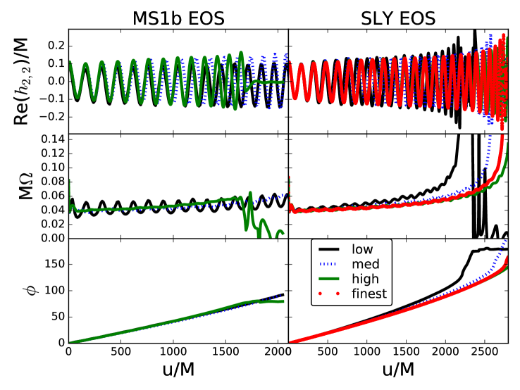
Figure 2: MHDuet evolutions for both EOSs and different resolutions. Between any two runs, the resolution increases by 25%. Quantities shown are the same ones shown in Fig. 1.

Figure 3: Strains for the highest resolution runs of the two different codes and two different EOSs.

Figure 4: Errors in phase between the different resolutions for the SLy MHDuet runs. Top: The strains for the four different resolutions. Middle: Differences in phase between successive resolutions. These differences decrease toward zero as resolution increases indicating convergence. Bottom: The convergence order estimated with just the phase differences, indicating high order convergence. The early significant variations are a consequence of differences being too small.

Figure 5: Phase errors relative to the Richardson extrapolated phase for the MHDuet SLy case. The differences between the extrapolated phase and the various resolutions are shown. That they decrease with resolution is another indication of convergence.

We can also analyze the various radiative quantities that are extracted on a spherical surface. We extract on three spherical surfaces at the different radii $r=\{350,450,600\}$ km, and plot those results for the finest resolution SLy run in Fig. 6. That these quantities largely agree gives some indication that their extraction is correct. We can make a quantitative statement by extrapolating the waveforms to infinity and subtracting each of the signals obtained on each surface. This measure indicates that the error due to the finite size extraction radii are much smaller than the discretization errors.

Figure 6: Results from the three different extraction surfaces for the finest SLy run. The top panel shows the strain and the bottom panel shows the differences between the phase obtained on each surface and the phase obtained by extrapolating to infinite radius with the outermost two surfaces.

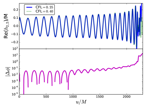
Figure 7: Phase error for the MHDuet SLy low resolution runs with two different CFL ratios. That the phase difference (shown in the bottom panel) is small, compared to Fig. 4, indicate that the use of a CFL factor of $0.40$ is not causing a large error in the solution. The ability to run with a high CFL factor is itself an efficient aspect of the MHDuet code.

Figure 8: Weak scaling test of the MHDuet code on stampede2 and comet. This run used fixed meshes with two levels. More recent tests have indicated (see Figure 15 of  Palenzuela:2018sly ) scaling efficiencies of 80% extend to at least 10,000 processes.

To examine the errors associated with our use of a large CFL factor $\lambda_{c}=0.4$ (as compared to other work using similar numerical schemes in this community Radice:2013xpa ; Bernuzzi:2016pie using $\lambda_{c}\approx 0.25$), we adopt these two values with a low resolution run of the SLy EOS with the MHDuet code and compare the results in Fig. 7. The phase difference between the two simulations suggests a small error until merger, as compared to the phase errors between different resolutions displayed in Fig. 4. This comparison further suggests that accurate (and efficient) simulations can be performed with the MHDuet code using such a large CFL factor.

IV Summary

We have presented binary neutron star simulations using two different EOS to compare two codes implemented in separate computational infrastructures. These codes solve the same evolution equations for both the Einstein and the MHD equations, and share the numerical schemes for smooth solutions. However, they implement different High-Resolution-Shock-Capturing methods: while Had uses an approach strongly inspired on finite-volume methods, where the fields are reconstructed at the interfaces and a flux-formula is used for calculating the fluxes at such interfaces, MHDuet relies on finite-difference methods, which involve a high order reconstruction of a combination of fluxes and fields (i.e., Lax-Friedrichs flux splitting). Another important difference is the treatment of the AMR boundaries, which is more efficient in MHDuet due to the use of a minimum bandwidth. Finally MHDuet is built using the public infrastructure Samrai, which has been developed for a number years and which can reach the exascale, at least for some choice of problems. For our main purposes, that of compact binary simulations, we have achieved good scaling up to 10,000 processes with our high-order schemes (see Fig. 8 for weak scaling results with up to 1,500 processes with the GRMHD code and Fig. 15 of Palenzuela:2018sly ).

The results presented here show several features. First, we have shown that the solutions of both codes are consistent and agree up to certain level. A more detailed analysis of one of these cases with MHDuet indicates that the solution roughly converges to fourth order. Richardson extrapolation allows us to estimate the errors in the phase, which remain below 0.2 radians for most of the coalescence for the highest resolution case with $\Delta x=160m$ and only increases to order unity in the last few orbits.

Another important technical result is that the speed and efficiency of the MHDuet code is better than Had, being able to achieve speeds of $\approx 20$ $M_{\odot}$/hour when running on 500-1000 processors for the highest resolution simulations of binary neutron stars presented here. This speed is roughly 4 times faster than the one reached by Had, which is moreover running at a resolution $\approx 15\%$ lower in our finest resolution comparison. For instance, on comparable architectures, MHDuet does roughly $85$ms per month running on 192 processors with a minimum resolution of $\Delta x=0.21$, while Had takes approximately $20$ms per month on 256 processors with even a slightly coarser minimum resolution of $\Delta x=0.25$.

Of course, much still needs to be added to MHDuet. In particular, the ability to handle tabulated equation of state, an approximate neutrino treatment and resistive magneto hydrodynamics, which are already available in Had. These physics ingredients are gradually being incorporated in MHDuet. Certainly, results presented here are encouraging for this enterprise.

- (1) M. Shibata and K. Hotokezaka, “Merger and mass ejection of neutron star binaries,” Annual Review of Nuclear and Particle Science 69 no. 1, (2019) 41–64, https://doi.org/10.1146/annurev-nucl-101918-023625. https://doi.org/10.1146/annurev-nucl-101918-023625.
- (2) D. Radice, S. Bernuzzi, and A. Perego, “The Dynamics of Binary Neutron Star Mergers and of GW170817,” arXiv:2002.03863 [astro-ph.HE].
- (3) J. M. Miller and E. Schnetter, “An operator-based local discontinuous Galerkin method compatible with the BSSN formulation of the Einstein equations,” Class. Quant. Grav. 34 no. 1, (2017) 015003, arXiv:1604.00075 [gr-qc].
- (4) F. Hébert, L. E. Kidder, and S. A. Teukolsky, “General-relativistic neutron star evolutions with the discontinuous Galerkin method,” Phys. Rev. D98 no. 4, (2018) 044041, arXiv:1804.02003 [gr-qc].
- (5) J. Piotrowska, J. M. Miller, and E. Schnetter, “Spectral Methods in the Presence of Discontinuities,” J. Comput. Phys. 390 (2019) 527–547, arXiv:1712.09952 [cs.NA].
- (6) A. G. M. Lewis and H. P. Pfeiffer, “GPU-accelerated simulations of isolated black holes,” Class. Quant. Grav. 35 no. 9, (2018) 095017, arXiv:1804.09101 [gr-qc].
- (7) M. Fernando, D. Neilsen, H. Lim, E. Hirschmann, and H. Sundar, “Massively Parallel Simulations of Binary Black Hole Intermediate-Mass-Ratio Inspirals,” arXiv:1807.06128 [gr-qc].
- (8) Dudi, Reetika and Pannarale, Francesco and Dietrich, Tim and Hannam, Mark and Bernuzzi, Sebastiano and Ohme, Frank and Bruegmann, Bernd, “Relevance of tidal effects and post-merger dynamics for binary neutron star parameter estimation,” Phys. Rev. D98 no. 8, (2018) 084061, arXiv:1808.09749 [gr-qc].
- (9) S. Bernuzzi and T. Dietrich, “Gravitational waveforms from binary neutron star mergers with high-order weighted-essentially-nonoscillatory schemes in numerical relativity,” Phys. Rev. D94 no. 6, (2016) 064062, arXiv:1604.07999 [gr-qc].
- (10) LIGO Scientific, Virgo Collaboration, B. P. Abbott et al., “Properties of the binary neutron star merger GW170817,” Phys. Rev. X9 no. 1, (2019) 011001, arXiv:1805.11579 [gr-qc].
- (11) D. Radice, A. Perego, F. Zappa, and S. Bernuzzi, “GW170817: Joint Constraint on the Neutron Star Equation of State from Multimessenger Observations,” Astrophys. J. 852 no. 2, (2018) L29, arXiv:1711.03647 [astro-ph.HE].
- (12) I. Harry and T. Hinderer, “Observing and measuring the neutron-star equation-of-state in spinning binary neutron star systems,” Class. Quant. Grav. 35 no. 14, (2018) 145010, arXiv:1801.09972 [gr-qc].
- (13) D. Alic, C. Bona-Casas, C. Bona, L. Rezzolla, and C. Palenzuela, “Conformal and covariant formulation of the Z4 system with constraint-violation damping,” Phys. Rev. D 85 no. 6, (Mar., 2012) 064040, arXiv:1106.2254 [gr-qc].
- (14) M. Bezares, C. Palenzuela, and C. Bona, “Final fate of compact boson star mergers,” Phys. Rev. D 95 (Jun, 2017) 124005. https://link.aps.org/doi/10.1103/PhysRevD.95.124005.
- (15) M. Anderson et al., “Simulating binary neutron stars: dynamics and gravitational waves,” Phys. Rev. D77 (2008) 024006, arXiv:0708.2720 [gr-qc].
- (16) D. Neilsen, S. L. Liebling, M. Anderson, L. Lehner, E. O’Connor, and C. Palenzuela, “Magnetized neutron stars with realistic equations of state and neutrino cooling,” Physical Review D 89 no. 10, (May, 2014) . http://dx.doi.org/10.1103/PhysRevD.89.104029.
- (17) G. Calabrese, L. Lehner, O. Reula, O. Sarbach, and M. Tiglio, “Summation by parts and dissipation for domains with excised regions,” Classical and Quantum Gravity 21 (Dec., 2004) 5735–5757, gr-qc/0308007.
- (18) G. Calabrese, L. Lehner, O. Reula, O. Sarbach, and M. Tiglio, “Summation by parts and dissipation for domains with excised regions,” Classical and Quantum Gravity 21 (Dec., 2004) 5735–5757, gr-qc/0308007.
- (19) C. Palenzuela, B. Miñano, D. Viganò, A. Arbona, C. Bona-Casas, A. Rigo, M. Bezares, C. Bona, and J. Massó, “A Simflowny-based finite-difference code for high-performance computing in numerical relativity,” Class. Quant. Grav. 35 no. 18, (2018) 185007, arXiv:1806.04182 [physics.comp-ph].
- (20) E. F. Toro, Riemann solvers and numerical methods for fluid dynamics: a practical introduction; 2nd ed. Springer, Berlin, 1999. http://cds.cern.ch/record/404378.
- (21) C.-W. Shu, Essentially non-oscillatory and weighted essentially non-oscillatory schemes for hyperbolic conservation laws, pp. 325–432. Springer Berlin Heidelberg, Berlin, Heidelberg, 1998. https://doi.org/10.1007/BFb0096355.
- (22) C. Palenzuela, S. L. Liebling, D. Neilsen, L. Lehner, O. L. Caballero, E. O’Connor, and M. Anderson, “Effects of the microphysical equation of state in the mergers of magnetized neutron stars with neutrino cooling,” Phys. Rev. D 92 no. 4, (Aug., 2015) 044045, arXiv:1505.01607 [gr-qc].
- (23) C.-W. Shu and S. Osher, “Efficient implementation of essentially non-oscillatory shock-capturing schemes,” J. Comput. Phys. 77 no. 2, (1988) 439–471.
- (24) P. Colella and P. R. Woodward, “The Piecewise Parabolic Method (PPM) for Gas-Dynamical Simulations,” Journal of Computational Physics 54 (Sept., 1984) 174–201.
- (25) A. Harten, P. D. Lax, and B. van Leer, “On upstream differencing and godunov-type schemes for hyperbolic conservation laws,” SIAM Review 25 no. 1, (1983) 35–61, https://doi.org/10.1137/1025002. https://doi.org/10.1137/1025002.
- (26) S. Gottlieb and C.-W. Shu, “Total variation diminishing runge-kutta schemes,” Math. Comput. 67 no. 221, (Jan., 1998) 73–85. https://doi.org/10.1090/S0025-5718-98-00913-2.
- (27) “Had.” http://had.liu.edu/.
- (28) S. L. Liebling, “Singularity threshold of the nonlinear sigma model using 3D adaptive mesh refinement,” Phys. Rev. D 66 no. 4, (Aug., 2002) 041703, gr-qc/0202093.
- (29) L. Lehner, S. L. Liebling, and O. Reula, “Amr, stability and higher accuracy,” Class. Quant. Grav. 23 (2006) S421–S446. gr-qc/0510111.
- (30) L. Lehner, S. L. Liebling, C. Palenzuela, and P. M. Motl, “m=1 instability and gravitational wave signal in binary neutron star mergers,” Phys. Rev. D94 no. 4, (2016) 043003, arXiv:1605.02369 [gr-qc].
- (31) L. Sagunski, J. Zhang, M. C. Johnson, L. Lehner, M. Sakellariadou, S. L. Liebling, C. Palenzuela, and D. Neilsen, “Neutron star mergers as a probe of modifications of general relativity with finite-range scalar forces,” arXiv:1709.06634 [gr-qc].
- (32) A. Arbona, A. Artigues, C. Bona-Casas, J. Massó, B. Miñano, A. Rigo, M. Trias, and C. Bona, “Simflowny: A general-purpose platform for the management of physical models and simulation problems,” Computer Physics Communications 184 (Oct., 2013) 2321–2331.
- (33) A. Arbona, B. Miñano, A. Rigo, C. Bona, C. Palenzuela, A. Artigues, C. Bona-Casas, and J. Massó, “Simflowny 2: An upgraded platform for scientific modelling and simulation,” Computer Physics Communications 229 (Aug., 2018) 170–181, arXiv:1702.04715 [cs.MS].
- (34) R. D. Hornung and S. R. Kohn, “Managing application complexity in the samrai object-oriented framework,” Concurrency and Computation: Practice and Experience 14 no. 5, (2002) 347–368. http://dx.doi.org/10.1002/cpe.652.
- (35) B. T. Gunney and R. W. Anderson, “Advances in patch-based adaptive mesh refinement scalability,” Journal of Parallel and Distributed Computing 89 (2016) 65 – 84. http://www.sciencedirect.com/science/article/pii/S0743731515002129.
- (36) P. McCorquodale and P. Colella, “A high-order finite-volume method for conservation laws on locally refined grids,” Commun. Appl. Math. Comput. Sci. 6 no. 1, (2011) 1–25. https://doi.org/10.2140/camcos.2011.6.1.
- (37) B. Mongwane, “Toward a Consistent Framework for High Order Mesh Refinement Schemes in Numerical Relativity,” Gen.Rel.Grav. 47 no. 5, (2015) 60, arXiv:1504.07609 [gr-qc].
- (38) D. Radice and L. Rezzolla, “THC: a new high-order finite-difference high-resolution shock-capturing code for special-relativistic hydrodynamics,” A&A 547 (Nov., 2012) A26, arXiv:1206.6502 [astro-ph.IM].
- (39) G.-S. Jiang and C.-W. Shu, “Efficient implementation of weighted eno schemes,” Journal of Computational Physics 126 no. 1, (1996) 202 – 228. http://www.sciencedirect.com/science/article/pii/S0021999196901308.
- (40) A. Suresh and H. Huynh, “Accurate monotonicity-preserving schemes with runge–kutta time stepping,” Journal of Computational Physics 136 no. 1, (1997) 83 – 99. http://www.sciencedirect.com/science/article/pii/S0021999197957454.
- (41) C. Bona, C. Bona-Casas, and J. Terradas, “Linear high-resolution schemes for hyperbolic conservation laws: TVB numerical evidence,” Journal of Computational Physics 228 (Apr., 2009) 2266–2281, arXiv:0810.2185 [gr-qc].
- (42) J. S. Read, B. D. Lackey, B. J. Owen, and J. L. Friedman, “Constraints on a phenomenologically parametrized neutron-star equation of state,” Physical Review D 79 no. 12, (Jun, 2009) . http://dx.doi.org/10.1103/PhysRevD.79.124032.
- (43) T. Dietrich, S. Bernuzzi, B. Bruegmann, and W. Tichy, “High-resolution numerical relativity simulations of spinning binary neutron star mergers,” in Proceedings, 26th Euromicro International Conference on Parallel, Distributed and Network-based Processing (PDP 2018): Cambridge, UK, March 21-23, 2018, pp. 682–689. 2018. arXiv:1803.07965 [gr-qc].
- (44) L. Baiotti, T. Damour, B. Giacomazzo, A. Nagar, and L. Rezzolla, “Accurate numerical simulations of inspiralling binary neutron stars and their comparison with effective-one-body analytical models,” Phys. Rev. D84 (2011) 024017, arXiv:1103.3874 [gr-qc].
- (45) D. Radice, L. Rezzolla, and F. Galeazzi, “High-Order Fully General-Relativistic Hydrodynamics: new Approaches and Tests,” Class. Quant. Grav. 31 (2014) 075012, arXiv:1312.5004 [gr-qc].