Connecting MapReduce Computations to
Realistic Machine Models

Abstract.

We explain how the popular, highly abstract MapReduce model of parallel computation (MRC) can be rooted in reality by explaining how it can be simulated on realistic distributed-memory parallel machine models like BSP. We first refine the model (MRC⁺) to include parameters for total work $w$, bottleneck work $\hat{w}$, data volume $m$, and maximum object sizes $\hat{m}$. We then show matching upper and lower bounds for executing a MapReduce calculation on the distributed-memory machine – $\Theta(w/p+\hat{w}+\log p)$ work and $\Theta(m/p+\hat{m}+\log p)$ bottleneck communication volume using $p$ processors.

1. Introduction

Figure 1. Several algorithmic measures are needed in order to robustly execute computations specified in the highly abstract MapReduce model on a realistic machine.

MapReduce (DeanGhemawat08, ) is a simple and successfull model for parallel computing. Tools like MapReduce/Hadoop, Spark or Thrill have “democratized” massively parallel computing. What was previously only used for numerical simulations that need investments of many person-years to get an application running is now used for a wide range of “big data” applications. Simple applications can be built within an hour and there is a rather gentle learning curve. One reason for this success is that a simple operation like the MapReduce transformation of multisets can express a large range of applications. The tools can automatically handle difficult issues like parallelization, load balancing, fault tolerance, and management of the memory hierarchy.

MapReduce steps get a multiset $A\subseteq I$ of elements from an input data type $A$ and map $A$ to a multiset of key–value pairs $B=\bigcup_{a\in A}\mu(a)\subseteq K\times V$ for a user-defined mapping function $\mu$. Next, values with the same key are collected together (shuffling), i.e., the system computes the set

$$C=\left\{(k,X):k\in K\wedge X=\left\{x:(k,x)\in B\right\}\wedge X\neq\emptyset\right\}\text{.}$$

Finally, a user defined reduction function $\rho$ is applied to the elements of $C$ to obtain an output multiset $D$. Representing the elements in $A$–$D$ may take variable space that we measure in machine words of a random access machine. Figure 1 summarizes the resulting logical data flow. The user only needs to specify $\mu$ and $\rho$; the system is taking care of the rest. Chaining several MapReduce steps with different mapping and reduction operations yields a wide spectrum of useful applications.

The MapReduce concept has been developed into a theoretical model of “big data” computations (MRC) (karloff:mapreduce, ) that is popular in the algorithm theory community. Problems are in MRC if they can be solved using a polylogarithmic number of MapReduce steps and if a set of (rather loose) additional constraints is fulfilled: Let $n$ denote the input size and $\epsilon>0$ some constant. The time for one invocation of $\mu$ or $\rho$ must be polynomial in $n$ using “substantially” sublinear space, i.e., $\mathrm{O}(n^{1-\epsilon})$. The overall space used for $B$ must be “substantially” subquadratic, i.e., $\mathrm{O}(n^{2-2\epsilon})$. While MRC has given new impulses to parallel complexity theory, it opens a gap between theory and practice. MRC based algorithms that use the full leeway of the model are unlikely to be efficient in practice. They are not required to achieve any speedup over the best practical sequential algorithm. They are also allowed to use near quadratic space so that they may not be able to solve large instances at all. There is also a possible bias that would prefer publications on impractical MRC-algorithms – practical ones are more likely to be similar to known algorithms in other parallel models and thus could be more difficult to publish.

However, we believe that a slightly more precise analysis can yield a model MRC⁺ that is more predictive for efficiency and scalability yet maintains the high level of abstraction of MRC. The main change is to not only count MapReduce steps but to also analyze work and communication volume based on the following four parameters: Let $w$ denote the total time needed to evaluate the functions $\mu$ and $\rho$ on all their inputs. Let $\hat{w}$ denote the maximum time for a single call to these functions. Let $m$ denote the total number of machine words contained in the sets $A$–$D$. Let $\hat{m}$ denote the maximum number of machine words produced or consumed by one call of the functions $\mu$ and or $\rho$.

The main contribution of this paper is to prove the following theorem about executing MapReduce computations on a distributed-memory machine with $p$ processing elements (PEs):

Theorem 1.1.

Assume that the input set $A$ of a MapReduce step is distributed over the PEs such that each PE stores $\mathrm{O}\!\left(m/p+\hat{m}\right)$ words of it. Then it can be implemented to run on a distributed-memory parallel computer with expected local work and bottleneck communication volume

(1) $$\mathrm{\Theta}\!\left(\frac{w}{p}+\hat{w}+\log p\right)\text{ and }\mathrm{\Theta}\!\left(\frac{m}{p}+\hat{m}+\log p\right)\text{,}$$

respectively. These bounds are tight, i.e., there exist inputs where no better bounds are possible. Moreover, no PE produces more than

$$\mathrm{O}\!\left(\sum_{d\in D}\frac{|d|}{p}+\max_{d\in D}|d|\right)=\mathrm{O}\!\left(\frac{m}{p}+\hat{m}\right)$$

words of output data.

Hence, the five parameters $w$, $\hat{w}$, $m$, $\hat{m}$, and $p$ govern the complexity of the algorithm in an easy to remember way. Note that the precondition and postcondition of Theorem 1.1 are formulated in such a way that multiple MapReduce steps can be chained.

Of course, there are middle-ways between the zero-parameter model of MRC and our proposed MRC⁺ model. We could impose the constraints $\hat{w}=\mathrm{O}\!\left(w/p\right)$ and $\hat{m}=\mathrm{O}\!\left(m/p\right)$, thus hiding the parameters $\hat{w}$ and $\hat{m}$ from the main bound. However, this would neglect that also inefficient MapReduce steps can be part of an overall efficient computation that consists of many steps. With Bound (1) we can prove overall efficiency by summing over all MapReduce steps of the application problem. We could also unify work and communication volume – effectively assuming that a constant number of machines words can be communicated in every clock cycle. However this neglects that large scale computations can only be efficient on practical machines when $m=o(w)$ (amarasinghe2009exascale, ; Borkar13, ). Thus MRC⁺ allows us to quantify the amount of locality present in the computations for evaluating $\mu$ and $\rho$.

We now proceed as follows: After a discussion of related work in Section 2, Section 3 derives the lower bounds. These are not surprising but, nevertheless, not completely trivial to derive. We gradually approach the correponding upper bounds. On the way, we develop several load balancing algorithms. Some of them may also be a basis for highly scalable in-memory implementations of MapReduce. The more theoretical ones may help to understand limitations of existing implementations with respect to scalability and robustness against difficult inputs.

In Section 4 we give an almost straightforward implementation based on randomized static load balancing in the framework of the BSP model (McC96, ). It achieves Bound (1) when $w=\mathrm{\Omega}\!\left(\hat{w}p\log p\right)$ and $m=\mathrm{\Omega}\!\left(\hat{m}p\log p\right)$. These constraints are a limitation when work or data are highly imbalanced, when $p$ is very large or when the inputs are relatively small. This is relevant for massively parallel applications when many MapReduce steps have to be executed. For example, this might be the case for online data analysis after each step of a massively parallel scientific simulation (wang2015smart, ).

We improve load balancing for mapping and reduction (Steps 1 and 3 in Figure 1) in Section 5. We design and analyze a distributed-memory work stealing algorithm that takes communication volume for task descriptions into account. This quite fundamental result seems to be new and may be of independent interest. In Section 6, we show how to efficiently allocate elements of $C$ to PEs using hashing and prefix sums (Step 2 in Figure 1). This is “almost” enough to establish Theorem 1.1. Indeed, it would suffice to prove execution time $\mathrm{O}\!\left(w/p+\hat{w}\right)$ assuming communication bandwidth proportional to the speed of local computations. However, for our more detailed analysis that separates local computation from (possibly slower) communication, it fails to establish the postcondition of Theorem 1.1. This problem can arise when one PE happens to map many elements that all emit a large amount of data. Similarly, the load balancer from Section 5 (Theorem 5) does not have a postcondition that matches the precondition of the shuffling step described in Section 6 (Lemma 6.1). In Section 7 we propose two algorithms that can solve this problem.

We conclude our paper with a discussion of possible future enhancements of our results in Section 8.

2. Related Work

The original implementations of MapReduce (DeanGhemawat08, ), [hadoop.apache.org] consider data sets that do not fit into main memory. Newer big data frameworks like Spark (Spark, ) or Thrill (Thrill, ) not only offer additional operations but also better exploit in-memory operation where the input and output of the MapReduce steps fits into the union of the local memories of the employed machines. This allows much higher performance, in particular when many subsequent steps have to be performed. Such in-memory implementations are the main focus of our paper.

Hoefler et al. (hoefler2009towards, ) discuss how MapReduce computations (e.g., (DeanGhemawat08, ; lee2012parallel, ; plimpton2011mapreduce, )) are commonly implemented in practice. Most of these approaches are less scalable and robust than the algorithms introduced here. They often have some kind of centralized control that would introduce $\mathrm{\Omega}\!\left(p\right)$ terms into Bound (1). Also, elements of $A$ or $C$ may be parcelled into packets that can destroy load balance when many expensive elements happen to fall in one packet. The efficient C++ based implementations MapReduce-MPI (plimpton2011mapreduce, ) and Thrill (Thrill, ) use approaches similar to our BSP algorithm but abstain from explicit randomization or redistribution. MR-MPI (mohamed2013mro, ) refines this by allowing overlapping of mapping and reduction to some extend. K MapReduce (matsuda2013k, ) and Mimir (gao2017mimir, ) explicitly target large supercomputers. K MapReduce addresses the tradeoff between communication bandwidth and startup latencies during the shuffling step. We avoid this important issue by only discussing communication volume and not startup latencies – viewing concrete implementations of general data exchange as a topic orthogonal to our paper. Berlińska and Drozdowski (BERLINSKA201814, ) empirically compare several centralized load balancing algorithms for the reduction step.

On the theory side, Goodrich et al. (goodrich2011sorting, ) introduce the parameters $m$ and $w$ and give lower bounds based on these parameters (although they do not elaborate how they arrive at the communication lower bound which we prove using expander graphs). They also introduce a parameter $M$ that bounds the input size of the reducers, thus covering a frequent source of bottlenecks in MapReduce algorithms. They do not explicitly consider bottleneck input sizes or computation times otherwise. Furthermore, they show simulations in the opposite direction as our paper, i.e., how machine models like CRCW PRAMs or BSP can be simulated using MapReduce calculations. Pace (pace2012bsp, ) explains how to execute MapReduce computations on BSP when all the task execution times are known.

3. Lower Bounds

It is clear that the total work $w$ has to be distributed over $p$ PEs such that at least one PE gets work $\mathrm{\Omega}\!\left(w/p\right)$. Similarly, some PE has to evaluate $\mu$ (or $\rho$) for the most expensive function evaluation. This implies a lower bound of $\mathrm{\Omega}\!\left(\hat{w}\right)$ for a MapReduce operation.

The lower bounds due to communication are slightly less obvious because we have to prove that not enough of the computations can be done locally – even with clever adaptive strategies. Consider the bipartite graph $(A\cup C,E)$ whose edges $(a,k)$ connects outputs of $\mu$ with keys in $C$. If this graph is an expander graph, a constant fraction of all elements of $B$ has to be communicated. Thus $\mathrm{\Omega}\!\left(w/p\right)$ is a lower bound for the bottleneck communication volume. Now consider an evaluation of $\rho$ that works on $\hat{m}$ key-value pairs emitted by $\hat{m}$ different evaluations of $\mu$. Since the mapper has no way to predict the output of $\mu$, these key-value pairs may all be on different PEs. This results in a lower bound of $\hat{m}$ on the bottleneck communication volume. Finally, latency $\mathrm{\Omega}\!\left(\log p\right)$ is already needed in order to synchronize the PEs after a MapReduce computation is finished.

4. Using the BSP Model

We now consider a simple implementation of a MapReduce operation in the BSP model that uses randomized static load balancing. Recall that the BSP model (McC96, ) considers globally synchronized super steps where a local computation phase is followed by a message exchange phase. A superstep takes time $w_{x}+L+hg$ where $w_{x}$ is the bottleneck work, $L$ is the latency parameter, $g$ is the gap parameter, and $h$ is the bottleneck communication volume, i.e., the maximum number of machine words communicated on any PE. The gap parameter allows us to put local work and communication cost into a single expression.

Our implementation consists of two supersteps and assumes a random distribution of the input set $A$. In the first superstep, each PE maps its local elements. It then sends a key-value pair $(k,v)\in B$ to PE $h(k)\in 1..p$ where $h$ is a hash function. In the second superstep, each PE assembles the received elements of $B$ to obtain set $C$. This can be done using a local hash table with one entry for each key. It then applies the reduction function $\rho$ to obtain the output set $D$. Whenever a call of $\rho$ produces more than one output element, all but one of these elements are sent to a random PE to establish a postcondition that the output is randomly distributed. This postcondition allows MapReduce steps to be chained without additional measures to establish the precondition of random data distribution. Figure 2 gives an example.

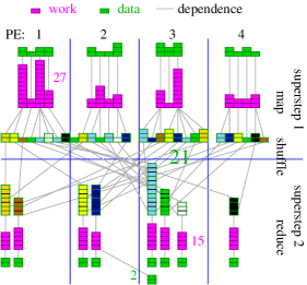
Figure 2. Example MapReduce problem with $m=146$, $\hat{m}=12$, $w=101$, and $\hat{w}=11$. Using the BSP algorithm on $p=4$ PEs, the bottleneck work for mapping is 27 units and 15 units for reducing. Bottleneck communication volume is 21 units for the first superstep and 2 for the second one.

Theorem 4.1.

Assume that the input set $A$ is randomly distributed over the PEs. Also assume that the hash function $h$ behaves like a truly random mapping. Then our BSP-based implementation takes expected time

(2) $$\mathrm{O}\!\left(\hat{w}\hat{o}\left(\frac{w}{\hat{w}},p\right)+L+g\hat{m}\hat{o}\left(\frac{m}{\hat{m}},p\right)\right)\text{,}$$

where $\hat{o}(b,p)$ denotes the expected maximum occupancy of a bin when randomly placing $\left\lceil b\right\rceil$ balls into $p$ bins (see (RaaSte98, ) for an exhaustive case distinction). In particular, the bound becomes

(3) $$\mathrm{O}\!\left(\frac{w}{p}+L+g\frac{m}{p}\right)\text{ if }w=\mathrm{\Omega}\!\left(\hat{w}p\log p\right)\text{ and }m=\mathrm{\Omega}\!\left(\hat{m}p\log p\right)\text{.}$$

Moreover, the output set $D$ is randomly distributed over the PEs.

Proof (Outline):   The local work for the first superstep is dominated by the maximum time for evaluating the mapping function $\mu$ for all elements assigned to a PE. The expectation for this maximum allocation is largest when the work is as skewed as possible, i.e., when the time for evaluating $\mu$ is zero except for $k=\left\lceil w/\hat{w}\right\rceil$ elements with required time $\hat{w}$; see (San96a, ). Thus, the expected maximum time can be bounded by $\hat{w}$ times the maximum occupancy of a bin when randomly allocating $k$ balls to $p$ bins. This is a well analyzed problem (RaaSte98, ). We get a bound of $\hat{w}\hat{o}(w/\hat{w},p)$ of local work for the first superstep.

The argument for the bottleneck communication volume of the first superstep is similar. Our precondition ensures that no evaluation of $\mu$ produces more than $\hat{m}$ machine words of data and the overall volume of produced data is at most $m$. We get bottleneck communication volume $\hat{m}\hat{o}(m/\hat{m},p)$ and therefore a term $g\hat{m}\hat{o}(m/\hat{m},p)$ for the communication cost of the first superstep.

By allocating elements of $C$ via random hashing, we ensure that also the executions of the reducer $\rho$ in the second superstep are randomly allocated to PEs. Thus we get analogous bounds as for the first superstep – invoking the analysis from (San96a, ; RaaSte98, ) both for the amount of received data and for the work performed by $\rho$. Using local hash tables, assembling the elements of $C$ can be done with expected work linear in the amount of received data.

Since $\hat{o}(x,p)=\mathrm{O}\!\left(x/p\right)$ for $x=\mathrm{\Omega}\!\left(p\log p\right)$, we also get Bound (3).

Finally, the postcondition is established by randomly dispersing data produced by reducers that emit more than one element of $D$ – the first emitted element is already randomly allocated thanks the the randomization through $h$. The resulting bottleneck communication volume is again implied by (San96a, ; RaaSte98, ) – both for the sent and received amount of data.

∎

5. Distributed Memory Work Stealing

In this section, we concentrate on the difficult load balancing problem of evaluating $\mu$ and $\rho$ in the absence of information on the cost of each function evaluation (job). The randomized static load balancing used in Section 4 cannot adapt to differences in the amount of work allocated to a PE. More generally, we have to avoid grouping jobs into parcels that have to be evaluated on the same PE before we know their cost. We also want to avoid bottlenecks such as in a master-worker load balancing scheme; e.g., (SMDD19, , Section 14.3).

We thus consider work-stealing load balancers (FinMan87, ; BluLei99, ; San02b, ) for handling the function evaluations of $\mu$ and $\rho$. They provide a highly scalable dynamic load balancing algorithm with adaptive granularity control. We overcome their restriction that they assume shared memory (BluLei99, ) or job descriptions that have fixed length (FinMan87, ; San02b, ). More concretely, we build on the asynchronous distributed-memory variant analyzed in (San02b, ). Instantiating this highly generic algorithm to our requirements, a piece of work represents a subarray of jobs. Splitting a subarray means sending away half its unprocessed jobs (never including the one that is currently being processed locally). Figure 3 gives an example.

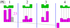
Figure 3. Continuation of the example from Figure 2 showing a possible impact of work stealing on the mapping step. After 10 units of local computation PE 4 might steal from PE 1. At that time PE 1 has already finished its first job and started on the first job. Thus it gives away half the remaining jobs which ist its fourth job. At the time further PEs get idle, PE 1 has already started its large third job. Thus further reductions of the bottleneck work cannot take place in this small instance.

Unfortunately, the result is not directly applicable since communicating a subarray of jobs entails communicating the descriptions of all the jobs it contains. Moreover, some jobs may be migrated up to $\log m$ times. We address this problem by initially locally sorting the jobs by approximately decreasing description length, i.e., PEs preferably process jobs with long description and communicate jobs with short description to save communication volume. With a generalized analysis, we obtain the following result that may be of independent interest.

Theorem 5.1.

Consider an array of independent jobs whose total description length is bounded by $m$ and where, initially, each PE locally stores jobs that can be described using $\mathrm{O}\!\left(m/p+\hat{m}\right)$ machine words. Let $w$ denote the total work needed to execute all the jobs and let $\hat{w}$ denote the maximum time needed to execute a single job. Then $p$ PEs can process all jobs using expected local work $\mathrm{O}\!\left(w/p+\hat{w}+\log p\right)$ and expected bottleneck communication volume $\mathrm{O}\!\left(m/p+\hat{m}+\log p\right)$.

Proof.

We only ouline how the analysis of (San02b, ) can be adapted. Using bucket sort by the value $\left\lfloor\log x\right\rfloor$ for a job of description length $x$, preprocessing is possible in time $\mathrm{O}\!\left(m/p+\log m\right)$ such that job sizes in each bucket differ by at most a factor of two.

Adapted to the notation used here, but ignoring the nonuniform communication costs, the outcome of the analysis from (San02b, ) is that local work $\mathrm{O}\!\left(w/p+\hat{w}\right)$ and bottleneck communication volume $\mathrm{O}\!\left(\log m\right)$ are sufficient. Transferring subarrays of jobs implies additional “dead times” during which migrating subarrays cannot be split. However, sorting ensures that the data volume in subsequent subarray migrations decreases at least geometrically. Hence, the overall migration volume (and the corresponding dead times) are linear in the original local data volume of one PE. Splitting always in half with respect to the number of remaining jobs ensures that there are at most $\log m$ generations. Overall, the dead times sum to

$$\mathrm{O}\!\left(\frac{m}{p}+\hat{m}+\log m\right)=\mathrm{O}\!\left(\frac{m}{p}+\hat{m}+\log p\right)\text{.}$$

The latter asymptotic estimate stems from the fact that $m/p+\log m=\mathrm{O}\!\left(m/p+\log p\right)$ – whenever $\log m=\omega(\log p)$ the term $m/p$ dominates $\log m$. ∎

6. Shuffling

Shuffling (Step 2 in Figure 1) has the task to establish two preconditions for efficiently performing the subsequent application of $\rho$ to all elements of $C$ (Step 3): All the data needed for each element of $C$ should be moved to the same PE, and, overall, each PE should receive $\mathrm{O}\!\left(m/p+\hat{m}\right)$ machine words of data. This is at the same time easier and more difficult than the load balancing problems from steps 1 and 3. It is easier because all the relevant data is available. It is more difficult, because this data is distributed over all PEs. We thus use a different load balancing algorithm here based on hashing and prefix sums.

The problem of the BSP algorithm from Section 4 is that the hash function with its range $1..p$ may map too many heavy elements of $C$ to the same PE. Hence, we use a two-stage approach. First, we hash keys to a larger range $1..m^{c}$ for a constant $c>2$. Hash values $h(c)$ in that range are unique with high probability (RaaSte98, ). We then aggregate the amount of data associated with the same $h(c)$. For each element $b=(k,x)\in B$, we move a pair $b^{\prime}=(h(k),|k|+|x|)$ to PE $i=h(k)\bmod p$. Note that the size of this pair is only a constant number of machine words. In contrast to the BSP algorithm, PE $i$ only aggregates the overall amount of data $v(c)$ needed for elements $c\in C$. Actually assigning elements of $c$ to PEs is done by computing a prefix sum over the $v(c)$ values. If the total size of elements in $C$ is $m^{\prime}$ and for an element $c\in C$ we have $\sum\left\{v(x):h(x)<h(c)\right\}=n$, we assign element $c$ to PE $1+\left\lfloor pn/m^{\prime}\right\rfloor$. Thus, each PE is assigned elements of $C$ with total volume $m^{\prime}/p+\mathrm{O}\!\left(\hat{m}\right)=\mathrm{O}\!\left(m/p+\hat{m}\right)$ with high probability. The PEs holding the input of the shuffling step are informed about these assignments by reply messages to the $b^{\prime}$ tuples. Thus, the actual data from $B$ is directly delivered to the PE that actually reduces it. Figure 4 gives an example. We obtain the following lemma:

Figure 4. Continuation of the example from Figure 2 showing a prefix-sum based shuffling step. The bottleneck communication volume is reduced from 21 to 18.

Lemma 6.1.

Suppose that before a shuffling step, the elements of $B$ are distributed in such a way that each PE holds data volume $\mathrm{O}\!\left(m/p+\hat{m}\right)$. Then shuffling can be implemented with expected local work and bottleneck communication volume $\mathrm{O}\!\left(m/p+\hat{m}+\log p\right)$. Moreover, each PE receives elements of $C$ with total volume $\mathrm{O}\!\left(m/p+\hat{m}\right)$.

Proof Outline:   The amount of data send in the counting step is $\mathrm{O}\!\left(m/p+\hat{m}\right)$ by the procondition. Using the same balls-into-bins notation as in Theorem 4.1, the expected amount of data received is $\leq\hat{o}(m,p)=\mathrm{O}\!\left(m/p+\log p\right)$. This communication is reversed later for comunicating the allocations of keys with the same asymptotic cost..

The prefix sum calculation needs work $\mathrm{O}\!\left(m/p+\log p\right)$ and bottleneck communication volume $\mathrm{O}\!\left(\log p\right)$. Actually delivering the data then incurs bottleneck communication volume $\mathrm{O}\!\left(m/p+\hat{m}\right)$. ∎

7. Establishing Postconditions

We propose two solutions to the problem outlined in the introduction because we want to illustrate the design landscape of scalable load balancing algorithms for MapReduce computations. We only describe what is done for balancing the output volume of the mapping step. The output of the reduction step can be balanced in an analogous fashion. Let $m^{\prime}$ denote the total data volume produced by the mapping step.

7.1. Redundant Remapping

Our first approach analyzes the situation after the mapping step. A remapping step is triggered if any PE has an output volume that significantly exceeds $m^{\prime}/p+\hat{m}^{\prime}$ where $\hat{m}^{\prime}\leq\hat{m}$ denotes the maximal output volume of a call to $\mu$. For a start, we consider a simple implementation that redos all the mapping calls after a data redistribution. Since here “all cards are on the table”, we can use a prefix sum based approach somewhat similar to Section 6. Each PE considers those elements it has processed locally. The only complication is that we have to balance input data volume, local computation, and output data volume simultaneously. We do this by appropriately scaling the values. Let $w^{\prime}$ denote the total time spent for mapping steps (this value can be measured during the initial execution of the mapping operation). For an element $a\in A$ with output data volume $o_{a}$, and work $w_{a}$, we compute a weight

$$W_{a}\mathbin{:=}w_{a}+o_{a}\frac{w^{\prime}}{m^{\prime}}\text{.}$$

Let $W\mathbin{:=}\sum_{a\in A}W_{a}$. Now we use prefix sums and data redistribution in order to assign to each PE elements with total weight $\sum_{a\in A}W/p$ plus possibly one further overload element. Figure 5 gives an example. Below we prove the following result:

Figure 5. Continuation of the example from Figure 2 Redistribution of the mapping computation based on a weighted sum of work and output volume.

Lemma 7.1.

Remapping can be implemented to run with local work $\mathrm{O}\!\left(w/p+\hat{w}+\log p\right)$ and bottleneck communication volume $\mathrm{O}\!\left(m/p+\hat{m}+\log p\right)$ such that no PE outputs more than $\mathrm{O}\!\left(m/p+\hat{w}\right)$ machine words of data.

Proof.

Since the redistribution only communicates the input data (which is balanced by the analysis of the previous operations), this can be done with time and communication volume $\mathrm{O}\!\left(m/p+\hat{m}+\log p\right)$ (see (HubSan15, ) for details of a data redistribution).

For the further analysis note that

$$W\mathbin{:=}\sum_{a\in A}W_{a}\!=\!\sum_{a\in A}\!w_{a}\!+\!o_{a}\frac{w^{\prime}}{m^{\prime}}\!=\!\sum_{a\in A}\!w_{a}\!+\!\frac{w^{\prime}}{m^{\prime}}\sum_{a\in A}\!o_{a}\!=\!w^{\prime}\!+\!m^{\prime}\frac{w^{\prime}}{m^{\prime}}\!=\!2w^{\prime}$$

and let $A_{i}$ denote the set of nonoverload input elements assigned to PE $i$. Data redistribution ensures that the elements in $A_{i}$ have total weight at most $W/p$.

Now, for any PE $i$, consider the local work $\sum_{a\in A_{i}}w_{a}$. We have

$$\sum_{a\in A_{i}}w_{a}\leq\sum_{a\in A_{i}}w_{a}+o_{a}\frac{w^{\prime}}{m^{\prime}}=\sum_{a\in A_{i}}W_{a}\leq\frac{W}{p}\leq 2\frac{w^{\prime}}{p}\text{.}$$

The overload element represents work at most $\hat{w}$ so that the local work within evaluations of $\mu$ is at most $2w^{\prime}/p+\hat{w}=\mathrm{O}\!\left(w/p+\hat{w}\right)$.

For the bottleneck communication volume $\sum_{a\in A_{i}}o_{a}$ observe that, similarly,

$$\sum_{a\in A_{i}}o_{a}\frac{w^{\prime}}{m^{\prime}}\leq\sum_{a\in A_{i}}W_{a}\leq 2\frac{w^{\prime}}{p}\text{.}$$

Multiplying this inequality with $m^{\prime}/w^{\prime}$ yields

$$\sum_{a\in A_{i}}o_{a}\frac{w^{\prime}}{m^{\prime}}\cdot\frac{m^{\prime}}{w^{\prime}}=\sum_{a\in A_{i}}o_{a}\leq 2\frac{w^{\prime}}{p}\cdot\frac{m^{\prime}}{w^{\prime}}=2\frac{m^{\prime}}{p}\text{.}$$

The overload element represents output data volume at most $\hat{m}$ so that the bottleneck output volume is at most $2m^{\prime}/p+\hat{m}=\mathrm{O}\!\left(m/p+\hat{m}\right)$. ∎

For the sake of a simple analysis, the above redistribution algorithms maps every element twice. This can be reduced by only redistributing some elements. More concretely, each PE identifies local elements whose total output data volume is above some threshold $bm^{\prime}/p$ and redistributes the excess to those PEs whose output data volume is lower. In (HubSan15, ) it is explained how this can be done efficiently using prefix sums, merging, and segmented gather/scatter operations.

7.2. Work Stealing with Strikes

We only outline the second approach which is a bit more complicated to analyze but indicates that the problem can be solved without redundant function evaluations. For a start, let us assume that the algorithm receives $m^{\prime}$ as an input. Then we can modify the work stealing load balancer from Section 5 so that a worker stops doing local work (it goes on strike) when it has produced more than $bm^{\prime}/p$ words of output for an appropriate constant $b>1$. From then on it does not send requests by itself. It answers work requests as before by splitting off half its remaining jobs. Since at most $p/b$ PEs can go on strike, the remaining $\mathrm{\Omega}\!\left(p\right)$ PEs can efficiently handle the remaining work. The assumption that $m^{\prime}$ is known can be lifted by estimating this value from a sample of mapper evaluations. We can also monitor the total produced data volume in the background and the PEs whose current volume significantly exceeds the current average go on strike (possibly temporarily).

8. Conclusions and Future Work

This paper closes gaps between MapReduce as an abstract model of computing (MRC$\rightarrow$MRC⁺) and realistic machine models. From a more practical perspective, our algorithms might also help to improve practical implementations.

Although our analysis neglects constant factors, our algorithms could be an interesting basis for practical implementations. Work stealing is an approach widely used in practice and allows low overhead adaptive load balancing. At least the variant from Section 7.2 performs no redundant function evaluations. The shuffling step moves the actual data only once in a single BSP-like data-exchange step. The additional counter-exchange step could be a significant overhead when the elements in $B$ are small. Here we could further optimize. For example, we could adapt the duplicate detection techniques from (SSM13, ) to reduce the data volume per element to a value close to $\log p$ bits. Further reductions might be possible by exploiting that it suffices to approximate the data allocation. For example, by only communicating an appropriate Bernoulli sample of the machine words used to represent $B$, we could achieve a good distributed approximation of the element sizes in $C$.

Our comparison to existing tools is unfair insofar as big data tools handle additional issues like fault-tolerance and I/O. Thus, studying generalizations of our algorithms is an interesting direction of future research – both theoretical and practical. We would like to have algorithms that tolerate errors like PE failures and that also balance fluctuations in the speed of PEs or communication links. Further, we would like to minimize I/O costs in an appropriate model of distributed external memory.

We can also look beyond MapReduce. At the same time as the MRC model has gained popularity as a theoretical model, practitioners have increasingly realized that plain MapReduce alone is not enough to implement a sufficiently wide range of applications efficiently. Breaking down an application into MapReduce steps often requires a large number of steps and thus complicates algorithm design. This is exacerbated by the requirement to communicate (and possibly move to/from external memory) basically all the involved data in every step. Even the original MapReduce publication (DeanGhemawat08, ) already introduces a more communication-efficient variant with reducers that allow local reduction of data with the same key, e.g., using a commutative, associative operator like $+$ or $\min$. More recent big data tools such as Spark (Spark, ), Flink (Flink, ), or Thrill (Thrill, ) adopt the highly abstract basic approach of MapReduce but offer additional operations and/or data types. For example, the Thrill framework (Thrill, ) is based on arrays and offers operations, for mapping, reducing, union, sorting, merging, concatenation, prefix sums, windows,…. The MRC⁺ model introduced above can be adapted to this approach. For each operation, we analyze its complexity in a realistic model of parallel computation and possibly simplify it to get rid of small but complicated factors that may be an artifact of the concrete implementation.

References

- [1] Saman Amarasinghe, Dan Campbell, William Carlson, Andrew Chien, William Dally, Elmootazbellah Elnohazy, Mary Hall, Robert Harrison, William Harrod, Kerry Hill, et al. Exascale software study: Software challenges in extreme scale systems. DARPA IPTO, Air Force Research Labs, Tech. Rep, pages 1–153, 2009.
- [2] Joanna Berlińska and Maciej Drozdowski. Comparing load-balancing algorithms for MapReduce under Zipfian data skews. Parallel Computing, 72:14–28, 2018.
- [3] T. Bingmann, M. Axtmann, E. Jöbstl, S. Lamm, H. Chau Nguyen, A. Noe, S. Schlag, M. Stumpp, T. Sturm, and P. Sanders. Thrill: High-performance algorithmic distributed batch data processing with C. In IEEE Conf. on Big Data (BigData), 2016.
- [4] R. D. Blumofe and C. E. Leiserson. Scheduling multithreaded computations by work stealing. Journal of the ACM, 46(5):720–748, 1999.
- [5] Shekhar Borkar. Exascale computing – a fact or a fiction? Keynote presentation at IPDPS 2013, Boston, May 2013.
- [6] Paris Carbone, Asterios Katsifodimos, Stephan Ewen, Volker Markl, Seif Haridi, and Kostas Tzoumas. Apache Flink: Stream and batch processing in a single engine. Bulletin of the IEEE Computer Society Technical Committee on Data Engineering, 36(4), 2015.
- [7] Jeffrey Dean and Sanjay Ghemawat. Mapreduce: simplified data processing on large clusters. Commun. ACM, 51:107–113, January 2008.
- [8] Martin Dietzfelbinger. On randomness in hash functions. In 29th Symposium on Theoretical Aspects of Computer Science (STACS), 2012.
- [9] R. Finkel and U. Manber. DIB – A distributed implementation of backtracking. ACM Trans. Prog. Lang. and Syst., 9(2):235–256, April 1987.
- [10] Tao Gao, Yanfei Guo, Boyu Zhang, Pietro Cicotti, Yutong Lu, Pavan Balaji, and Michela Taufer. Mimir: Memory-efficient and scalable mapreduce for large supercomputing systems. In 2017 IEEE International Parallel and Distributed Processing Symposium (IPDPS), pages 1098–1108. IEEE, 2017.
- [11] Michael T Goodrich, Nodari Sitchinava, and Qin Zhang. Sorting, searching, and simulation in the mapreduce framework. In International Symposium on Algorithms and Computation (ISAAC), volume 7074 of LNCS, pages 374–383. Springer, 2011.
- [12] Torsten Hoefler, Andrew Lumsdaine, and Jack Dongarra. Towards efficient mapreduce using mpi. In European Parallel Virtual Machine/Message Passing Interface Users’ Group Meeting, pages 240–249. Springer, 2009.
- [13] Lorenz Hübschle-Schneider, Peter Sanders, and Ingo Müller. Communication efficient algorithms for top- selection problems. CoRR, abs/1502.03942, 2015.
- [14] Howard J. Karloff, Siddharth Suri, and Sergei Vassilvitskii. A model of computation for mapreduce. In 21st ACM-SIAM Symposium on Discrete Algorithms (SODA), pages 938–948, 2010.
- [15] Kyong-Ha Lee, Yoon-Joon Lee, Hyunsik Choi, Yon Dohn Chung, and Bongki Moon. Parallel data processing with mapreduce: a survey. AcM sIGMoD Record, 40(4):11–20, 2012.
- [16] Motohiko Matsuda, Naoya Maruyama, and Shin’ichiro Takizawa. K MapReduce: A scalable tool for data-processing and search/ensemble applications on large-scale supercomputers. In 2013 IEEE International Conference on Cluster Computing (CLUSTER), pages 1–8. IEEE, 2013.
- [17] W. F. McColl. Scalable computing. In Computer Science Today, number 1000 in LNCS, pages 46–61. Springer, 1996.
- [18] Hisham Mohamed and Stéphane Marchand-Maillet. Mro-mpi: Mapreduce overlapping using mpi and an optimized data exchange policy. Parallel Computing, 39(12):851–866, 2013.
- [19] Matthew Felice Pace. Bsp vs mapreduce. Procedia Computer Science, 9:246–255, 2012.
- [20] Steven J Plimpton and Karen D Devine. Mapreduce in mpi for large-scale graph algorithms. Parallel Computing, 37(9):610–632, 2011.
- [21] M. Raab and A. Steger. “balls into bins” – A simple and tight analysis. In RANDOM: International Workshop on Randomization and Approximation Techniques in Computer Science, volume 1518, pages 159–170. LNCS, 1998.
- [22] P. Sanders. On the competitive analysis of randomized static load balancing. In S. Rajasekaran, editor, 1st Workshop on Randomized Parallel Algorithms, Honolulu, 1996.
- [23] Peter Sanders. Randomized receiver initiated load balancing algorithms for tree shaped computations. The Computer Journal, 45(5):561–573, 2002.
- [24] Peter Sanders, Kurt Mehlhorn, Martin Dietzfelbinger, and Roman Dementiev. Sequential and Parallel Algorithms and Data Structures – The Basic Toolbox. Springer, 2019.
- [25] Peter Sanders, Sebastian Schlag, and Ingo Müller. Communication efficient algorithms for fundamental big data problems. In IEEE Int. Conf. on Big Data, pages 15–23, 2013.
- [26] Yi Wang, Gagan Agrawal, Tekin Bicer, and Wei Jiang. Smart: A MapReduce-like framework for in-situ scientific analytics. In Int. Conference for High Performance Computing, Networking, Storage and Analysis, pages 1–12, 2015.
- [27] Matei Zaharia, Mosharaf Chowdhury, Michael J Franklin, Scott Shenker, and Ion Stoica. Spark: Cluster computing with working sets. In 2nd USENIX Conference on Hot Topics in Cloud Computing, HotCloud’10, 2010.