A Neural Network Based on First Principles

Abstract

In this paper, a Neural network is derived from first principles, assuming only that each layer begins with a linear dimension-reducing transformation. The approach appeals to the principle of Maximum Entropy (MaxEnt) to find the posterior distribution of the input data of each layer, conditioned on the layer output variables. This posterior has a well-defined mean, the conditional mean estimator, that is calculated using a type of neural network with theoretically-derived activation functions similar to sigmoid, softplus, and relu. This implicitly provides a theoretical justification for their use. A theorem that finds the conditional distribution and conditional mean estimator under the MaxEnt prior is proposed, unifying results for special cases. Combining layers results in an auto-encoder with conventional feed-forward analysis network and a type of linear Bayesian belief network in the reconstruction path.

Index Terms—  Neural networks, Maximum Entropy, Activation Functions, Projected Belief Network

1 Introduction

1.1 Motivation

Despite the brilliant success of deep networks, networks and their activation functions are generally selected empirically to learn general functions [1, 2]. In generative networks, the activation functions revolve around approximating the expected value of generating distributions that are selected for tractability [3, 4, 5] or are empirically determined [6]. Despite the elegant mathematical formulations, restricted Boltzmann machines (RBMs) [7], and variation autoencoders [8], the models are also selected based on tractability or empirical performance. This paper seeks to derive the network structure and activation function from first principles by deducing the network structure from the a posteriori distribution of the visible data given the layer output.

1.2 Problem Statement

Figure 1 illustrates the main ideas of this paper.

Fig. 1: Block diagram.

The diagram shows two network layers, but we will focus on just the first layer for now. The input to a network layer is a high-dimensional vector ${\bf x}\in\mathbb{R}^{N}$. A lower-dimensional feature is computed by linear transformation, ${\bf z}={\bf W}^{\prime}{\bf x}$, where ${\bf z}\in\mathbb{R}^{M}$ , and $M<N$.

A bias and activation function are applied prior to the next layer, but this is not relevant to analyzing the first layer. For now, the question is what can be inferred about $p({\bf x})$ from ${\bf z}$, bypassing layer 2 (See “bypass” in Fig. 1). The remaining components in layer 1 are described below and layer 2 is explained in Section 4.

2 Mathematical Approach

2.1 Prior Distribution

The prior (a priori distribution) $p_{0}({\bf x})$ quantifies the expectation about ${\bf x}$ before feature ${\bf z}$ is measured. The principle of maximum entropy (MaxEnt) [9] proposes that the entropy of a distribution, given by $H\{p({\bf x})\}=-\int_{{\bf x}}\;p({\bf x})\;\log(p({\bf x}))\;{\rm d}{\bf x}$ should be as high as possible subject to the known constraints. These distributions are generally of the exponential class [10]. Consider the following univariate exponential class of distributions:

$$\log p(x;\alpha)=\alpha x+bx^{2}-\log Z(\alpha),\vspace{-.1in}$$ (1)

where the dependence on $b$ has been removed from the notation because it is fixed by the choice of prior. Parameter $\alpha$ plays a special role because it controls the distribution mean. Let the expected value of distribution (1) be written

$$\lambda(\alpha)\stackrel{{\scriptstyle\mbox{\tiny$\Delta$}}}{{=}}\mathbb{E}\{x;\alpha\}=\int_{x}\;x\;p(x;\alpha)\;{\rm d}x.\vspace{-.1in}$$ (2)

In keeping with maximum entropy, $p_{0}({\bf x})$ should be constructed from $N$ independent univariate distributions (1) as follows

$$\log p_{0}({\bf x})=\sum_{i=1}^{N}\;\log p(x_{i};\alpha_{0}).$$ (3)

This class includes independent and identically distributed (iid) Gaussian, exponential, and their truncated variants, and they have highest entropy among all multivariate distributions under constraints that will be proposed.

2.2 Manifold Distribution

Conditioned on knowing ${\bf z}$, ${\bf x}$ can only exist on the set

$${\cal M}({\bf z})=\{{\bf x}:{\bf W}^{\prime}{\bf x}={\bf z}\}.$$ (4)

This is the set (a manifold) of all possible values of ${\bf x}$ that exactly reproduce the measured value ${\bf z}$. The posterior is therefore a manifold distribution

$$p({\bf x}|{\bf z})=p_{0}({\bf x})/\left(\int_{{\bf x}\in{\cal M}({\bf z})}\;p_{0}({\bf x})\;{\rm d}{\bf x}\right),\;\;\;{\bf x}\in{\cal M}({\bf z}),$$ (5)

which is $p_{0}({\bf x})$ projected onto the manifold, then normalized so it integrates to 1. To draw samples from (5), samples are drawn from the manifold ${\cal M}({\bf z})$ with probability proportional to the value of the prior distribution $p_{0}({\bf x})$. It can be shown [11] that the denominator in (5) can be written

$$\int_{{\bf x}\in{\cal M}({\bf z})}\;p_{0}({\bf x})\;{\rm d}{\bf x}=p_{0}({\bf z}),$$

which is the prior feature distribution, i.e. distribution of ${\bf z}$ under the assumption that ${\bf x}\sim p_{0}({\bf x})$. Rewriting (5),

$$p({\bf x}|{\bf z})=\frac{p_{0}({\bf x})}{p_{0}({\bf z})},\;\;\;{\bf x}\in{\cal M}({\bf z}).$$ (6)

Due to conditioning on ${\bf z}$, the denominator has a fixed value, so the manifold distribution is shaped only by $p_{0}({\bf x})$. This quantity is known in the method of PDF projection [12, 11]. The conditional mean estimate is the mean of (5), written

$$\bar{{\bf x}}_{z}\stackrel{{\scriptstyle\mbox{\tiny$\Delta$}}}{{=}}{\displaystyle\int_{{\bf x}\in{\cal M}({\bf z})}{\bf x}\;p({\bf x}|{\bf z}){\rm d}{\bf x}}.\vspace{-.1in}$$ (7)

2.3 Main Result

Despite the simple form of (6), it is not useful for sampling and (7) is not tractable. Also, (6) is not even a proper distribution, having infinite density on an infinitely thin manifold. To find a proper distribution that approximates (5), we use a surrogate density [13], which is a proper distribution that shares the properties of (5), which are (a) probability mass concentrated on the manifold ${\cal M}({\bf z})$, (b) mean $\bar{{\bf x}}_{z}\in{\cal M}({\bf z})$ (because ${\cal M}({\bf z})$ is convex), and (c) density on the manifold proportional to $p_{0}({\bf x})$. The following theorem gives form to the surrogate density.

Theorem 1

Let prior $p_{0}({\bf x})$ be written as (3) with univariate densities $p(x;\alpha_{0})$ of class (1) with mean $\lambda(\alpha_{0})$. Then, the surrogate density for $p({\bf x}|{\bf z})$ can be written

$$\log p({\bf x};\mbox{\boldmath$\alpha$}_{0}+\mbox{\boldmath$\alpha$})=\sum_{i=1}^{N}\;\log p(x_{i};\alpha_{0}+\alpha_{i}),\vspace{-.1in}$$ (8)

where $\mbox{\boldmath$\alpha$}={\bf W}{\bf h},$ and ${\bf h}$ is the solution of

$${\bf W}^{\prime}\lambda\left(\mbox{\boldmath$\alpha$}_{0}+{\bf W}{\bf h}\right)={\bf z}.$$ (9)

Furthermore, the mean of $p({\bf x};\mbox{\boldmath$\alpha$}_{0}+\mbox{\boldmath$\alpha$})$ equals

$$\hat{{\bf x}}_{z}=\lambda(\mbox{\boldmath$\alpha$}_{0}+{\bf W}{\bf h}).$$ (10)

Outline of Proof:. To show that solution ${\bf h}$ solving (9) exists, it is shown below that (9) is the same as the saddle point (SP) equation for the SP expansion of $p_{0}({\bf z})$. Since for the exponential family (1), the SP expansion exists over the entire range of ${\bf z}$ (see [14] appendix), the solution exists whenever ${\bf z}$ is valid, i.e. whenever ${\bf z}={\bf W}^{\prime}{\bf x}$ for a sample ${\bf x}$ in the support of $p_{0}({\bf x})$. Since $\hat{{\bf x}}_{z}=\lambda\left(\mbox{\boldmath$\alpha$}_{0}+\mbox{\boldmath$\alpha$}\right)$, ${\bf W}^{\prime}\bar{{\bf x}}_{z}={\bf z},$ meeting property (b) for a surrogate density. Using (3),(1), the gradient of $\log p({\bf x};\mbox{\boldmath$\alpha$}_{0}+\mbox{\boldmath$\alpha$})$ with respect to ${\bf x}$ is $\left[\frac{\partial\log p({\bf x};\mbox{\boldmath$\alpha$}_{0}+\mbox{\boldmath$\alpha$})}{\partial{\bf x}}\right]=\mbox{\boldmath$\alpha$}_{0}+\mbox{\boldmath$\alpha$}+2b{\bf x}.$ In order that (8) is proportional to $p_{0}({\bf x})$ on the manifold, it is necessary that the component of this gradient in any direction parallel to the manifold (i.e. orthogonal to columns of ${\bf W}$) is the same as for the prior $p_{0}({\bf x})$. This can be mathematically written ${\bf B}^{\prime}\left[\mbox{\boldmath$\alpha$}_{0}+\mbox{\boldmath$\alpha$}+2b{\bf x}\right]={\bf B}^{\prime}\left[\mbox{\boldmath$\alpha$}_{0}+2b{\bf x}\right],$ for orthonormal matrix ${\bf B}$ spanning the linear subspace orthogonal to the columns of ${\bf W}$. Therefore, $\alpha$ must be fully orthogonal to ${\bf B}$, and of the form $\mbox{\boldmath$\alpha$}={\bf W}{\bf h}$. This fulfills property (c) of the surrogate density. To fulfill property (a), it can be shown that the probability mass of the surrogate density indeed converges to the manifold for large $N$ (see [13], Appendix A).

To see how Theorem 10 defines a neural network, we first simplify notation, by defining the function ${\bf z}=\gamma({\bf h})={\bf W}^{\prime}\lambda\left({\bf W}{\bf h}\right)$ and its inverse: ${\bf h}=\gamma^{-1}({\bf z}).$ The concept of $\gamma^{-1}({\bf z})$ is illustrated in Figure 1. Feature ${\bf z}$, is converted to ${\bf h}$ through $\gamma^{-1}({\bf z})$, then multiplied by ${\bf W}$ to raise the dimension back to $N$, and finally passed through activation function $\lambda(\;)$ to produce $\bar{{\bf x}}_{z}$. Optionally, it can be passed to the generating distributions $p({\bf x};\mbox{\boldmath$\alpha$}_{0}+\mbox{\boldmath$\alpha$})$ for stochastic generation. According to the definition of $\gamma^{-1}(\;)$, ${\bf W}^{\prime}\bar{{\bf x}}_{z}={\bf z},$ or in other words, the feature ${\bf z}$ is recovered exactly when $\bar{{\bf x}}_{z}$ is processed by the forward path, illustrated in the figure where ${\bf z}$ of the forward path is identified with ${\bf z}$ produced by the circular path. In this role, $\gamma^{-1}({\bf z})$ acts as a non-linearity (but is not applied element-wise). Despite the iterative solution of $\gamma^{-1}({\bf z})$, its derivatives are easly calculated from $\gamma({\bf h})$, so are amenable to back-propagation training for optmizing the network parameters.

Since $\hat{{\bf x}}_{z}$ is the conditional mean estimator, it enjoys numerous optimal properties such as minimum mean square estimator [15]. Since the surrogate density converges to the posterior $p({\bf x}|{\bf z})$, it implies that $\hat{{\bf x}}_{z}\rightarrow\bar{{\bf x}}_{z}$ for large $N$. This convergence occurs quickly and low dimension as has been demonstrated in certain cases (see fig. 8 in [13]). In fact, $\hat{{\bf x}}_{z}=\bar{{\bf x}}_{z}$ under certain symmetry conditions. A special case of (10) corresponds to autoregressive spectral estimation, which can be generalized for conditioning on any linear function of the spectrum, such as MaxEnt inversion of MEL band features [13]. Another special case of (10) is mathematically the same as classical maximum entropy image reconstruction [16, 17]. It is also not surprising, given form (6), that the surrogate density has a close relationship to $p_{0}({\bf z})$. It can be shown that ${\bf h}$ is also the saddlepoint for the SP approximation to $p_{0}({\bf z})$. This can be seen by comparing (9) with equation 25 in [18], page 2245, which is the general SP equation for the linear sum of independent random variables. It can also be shown that ${\bf h}$ is the maximum likelihood estimate under the likelihood function (8) [14].

3 Three cases of $\mathbb{X}$

The MaxEnt prior $p_{0}({\bf x})$ depends on the range of ${\bf x}$, denoted by $\mathbb{X}$, and any other assumptions. The choice of $p_{0}({\bf x})$ in turn determines the activation function $\lambda(\alpha)$ and how to sample from the manifold ${\cal M}({\bf z})$. Whereas manifold sampling is exact sampling of $p({\bf x}|{\bf z})$, sampling from the surrogate density is an approximation. However, experiments have demonstrated the almost perfect correspondence between the two distributions (e.g. Figures 8,10,11 in [19]).

3.1 Unit hypercube $\mathbb{U}^{N}$

In the unit hypercube, denoted by $\mathbb{U}^{N}$, elements of ${\bf x}$ are in the range $[0,\;1]$, the case for intensity images, or if ${\bf x}$ is the output of a sigmoid activation function. The uniform prior is the MaxEnt distribution in $[0,\;1]$, $p_{0}({\bf x})=1$, which is the trivial case of (1) with $\alpha_{0}=0$, $b=0$. Sampling from ${\cal M}({\bf z})$ uniformly within $\mathbb{U}^{N}$ is done using a type of Monte Carlo Markov chain (MCMC) called hit-and-run [20], with modification for $\mathbb{U}^{N}$ as explained in detail in ([13], Sec. V, p. 2465). The surrogate density is a truncated exponential distribution (TED) $p(x;\alpha)=\frac{\alpha}{e^{\alpha}-1}\;e^{\alpha x},\;\;0>x>1$. The activation function is the TED nonlinearity [21, 13]

$$\lambda(\alpha)=\frac{e^{\alpha}}{e^{\alpha}-1}-\frac{1}{\alpha}$$ (11)

which resembles the sigmoid (see Fig. 2). This problem has been studied in detail in ([13], Sec. V, p. 2465).

3.2 Positive Quadrant $\mathbb{P}^{N}$

We assume that elements of ${\bf x}$ are positive, so exist in the positive quadrant of $\mathbb{R}^{N}$, denoted by $\mathbb{P}^{N}$. This happens if ${\bf x}$ is the output of an previous network layer and a rectifying activation function was used, or if ${\bf x}$ is some kind of spectral or intensity data that is inherently positive. There is no proper MaxEnt distribution on the open interval $[0,\;\infty]$ without constraining the mean or variance, resulting in two solutions. The constrained mean case results in an exponential prior and has been studied in detail ([13], Sec. IV, p. 2460). Although it corresponds to MaxEnt image reconstruction [16, 17], it is less interesting for neural networks.

If we are willing to assume a fixed variance, the truncated Gaussian with mean parameter 0 and variance parameter 1 (not the same as mean 0 and variance 1) provides the distribution with maximum entropy on $[0,\;\infty]$ [10]. This is the case of (1) with $\alpha_{0}=0$, $b=1$. This can also be written

$$p_{0}({\bf x})=\prod_{i=1}^{N}\;2{\cal N}(x_{i}),\;\;\;x_{i}>0,\forall i,\vspace{-.2cm}$$ (12)

where ${\cal N}(x)=\frac{e^{-x^{2}/2}}{\sqrt{2\pi}}.$ To sample ${\cal M}({\bf z})$ with this prior, an MCMC method similar to the exponential case (given in ([13], Sec. IV, p. 2460) can be used. A program implementing this procedure is provided in the appendix. The activation function is the mean of the truncated Gaussian:

$$\lambda(\alpha)=\alpha+\frac{{\cal N}(\alpha)}{\Phi(\alpha)}\vspace{-.1cm}$$ (13)

which resembles softplus (see Figure 2).

3.3 Unconstrained $\mathbb{R}^{N}$

There is no proper MaxEnt distribution on the open interval $[-\infty,\;\infty]$ without constraining the variance. In many cases, data has been normalized, so we are justified in using a standard Gaussian prior, which is the MaxEnt distribution on $\mathbb{R}^{N}$ for known variance [10]. For this case, the surrogate density is the same as the exact posterior. All samples on the manifold ${\cal M}({\bf z})$ can be written ${\bf x}=\bar{{\bf x}}_{z}+{\bf B}{\bf u},$ where $\bar{{\bf x}}_{z}={\bf W}{\bf h}$. and ${\bf B}$ is the same as in the proof of Theorem 10. This case is particularly instructive because $\gamma^{-1}({\bf z})$ has the closed-form expression $\gamma^{-1}({\bf z})=\left({\bf W}^{\prime}{\bf W}\right)^{-1}{\bf z},$ so applying $\gamma^{-1}({\bf z})$ corresponds to least-squares. To conform to the assumed prior distribution, ${\bf u}$ is a set of $(N-M)$ independent Gaussian random variables of zero mean and variance 1. The activation function is linear, $\lambda(x)=x$.

3.4 Summary and Remarks

Above results are summarized in the following table for four combinations of $\mathbb{X}$, and constraints (Const.). For each case, the table provides the MaxEnt prior $p_{0}({\bf x})$, the univariate distribution $p(x;\alpha)$ used to form the surrogate posterior (8), and the mean function $\lambda(\alpha)$.

$\mathbb{X}$	Const.	$p_{0}({\bf x})$	$p(x;\alpha)$	$\lambda(\alpha)$
$\mathbb{U}^{N}$	N/A	1	$\frac{\alpha}{e^{\alpha}-1}\;e^{\alpha x}$	$\frac{e^{\alpha}}{e^{\alpha}-1}-\frac{1}{\alpha}$
$\mathbb{P}^{N}$	$\mathbb{E}(x)$	$e^{-x}$	$\alpha e^{-\alpha x}$	${1\over\alpha}$
$\mathbb{P}^{N}$	$\mathbb{E}(x^{2})$	$2{\cal N}\left(x\right)$	$\frac{{\cal N}\left(x-\alpha\right)}{\Phi\left(\alpha\right)}$	$\alpha+\frac{{\cal N}(\alpha)}{\Phi(\alpha)}$
$\mathbb{R}^{N}$	$\mathbb{E}(x^{2})$	${\cal N}\left(x\right)$	${\cal N}\left(x-\alpha\right)$	$\alpha$

where ${\cal N}\left(x\right)\stackrel{{\scriptstyle\mbox{\tiny$\Delta$}}}{{=}}\frac{e^{-x^{2}/2}}{\sqrt{2\pi}}$ and $\Phi\left(x\right)\stackrel{{\scriptstyle\mbox{\tiny$\Delta$}}}{{=}}\int_{-\infty}^{x}{\cal N}\left(x\right).$

The functions $\lambda(\alpha)$ are the MaxEnt “activation functions” and resemble commonly-used functions (see Fig. 2). Note that the truncated Gaussian (TG) nonlinearity approaches the rectified linear unit (RELU) as the assumed variance of the prior (normally equal to 1) goes to zero.

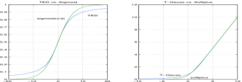
Fig. 2: Left: TED activation compared to Sigmoid. Right: TG activation compared to Softplus.

Alternatively, $\lambda(\;)$ can be replaced by the generating distribution $p({\bf x};\mbox{\boldmath$\alpha$}_{0}+\mbox{\boldmath$\alpha$})$ for stochastic generation. For a single layer, this would produce an RBM with deterministic forward path.

4 Building a Network

In Figure 1, a 2-layer network is created by adding another MaxEnt layer. The forward path (top) is a standard feed-forward network employing the MaxEnt activation functions. The data is first passed through a bias and activation function $\lambda_{2}(\;)$ before being presented to the second layer’s linear transform. Note that after layer 2 reconstructs its input in the backward path ($\bar{{\bf x}}_{z(2)}$) the activation function $\lambda_{2}(\;)$ and bias must be inverted before being processed by $\gamma^{-1}$. However, because the forward activation function $\lambda_{2}(\;)$ is the same as the MaxEnt activation function for layer 2, then $\lambda_{2}(\;)$ cancels $\lambda_{2}^{-1}(\;)$, resulting in a simplified backward path (see short dotted line at the bottom of the figure). It is also worth noting that in the backward (reconstruction) path, stochastic generation using $p({\bf x};\mbox{\boldmath$\alpha$}_{0}+\mbox{\boldmath$\alpha$})$ can be used in place of activation functions to create stochastic networks.

The reverse path (bottom) consists of applying $\gamma^{-1}({\bf z})$ (after removal of bias, if needed), followed by dimension-increasing transformation by the layer weight matrices (same matrix used in the forward path). This eliminates the need for separate reconstruction weights, and decreases network parameter count. This has been called a deterministic projected belief network [19, 22].

Although the existence of ${\bf h}=\gamma^{-1}({\bf z})$ is guaranteed for a single layer, it is not guaranteed for multiple layers. In other words, if ${\bf z}$ applied to $\gamma^{-1}$ is derived from the second layer and not from the forward path of the first layer, then ${\bf h}=\gamma^{-1}({\bf z})$ is not guaranteed to exist. This is the sampling efficiency issue on projected belief networks [21]. It has been experimentally shown that as a PBN is trained, the sampling efficiency approaches 1.0 [21].

5 Conclusions

In this paper, a new theorem has been presented that provides a closed-form asymptotic (large $N$) expression for the conditional mean $\bar{{\bf x}}_{z}=\mathbb{E}\{{\bf x}|{\bf z}\}$ given the output ${\bf z}$ of a dimension-reducing linear transformation under a class of MaxEnt prior distributions. The computation of the conditional mean resembles a linear Bayesian belief network layer with special non-linear function preceding the linear transformation and special activation function. Methods to sample the posterior $p({\bf x}|{\bf z})$ are provided. Applying this concept results in an auto-endoding neural network based on first principles.

[ Appendix: Sampling from ${\cal M}({\bf z})$ under the truncated Gaussian Prior] Let ${\bf B}$ be the same as in the proof of Theorem 10, so is a $N\times(N-M)$ orthonormal matrix orthogonal to ${\bf W}$. Let ${\bf x}$ be an $N\times 1$ vector, that is a member of ${\cal M}({\bf z})$, so ${\bf W}^{\prime}{\bf x}={\bf z}.$ The following procedure will find a new candidate ${\bf x}$, and if used repeatedly, will generate samples distributed according to (6) with $p_{0}({\bf x})$ as given by (12). The following MATLAB program will generate samples in $\mathbb{P}^{N}$ and in ${\cal M}({\bf z})$ uniformly or according to the truncated Gaussian prior (see comments).

function x=ums_tgauss_iter(x,B);
   [n,bdim]=size(B);
   bu=zeros(bdim,1);
   if(any(x<=0)), error(’invalid data’) end;
   for j=1:bdim,
      xu = B(:,j)./x;
      maxuneg=-1/max(xu);
      maxupos=-1/min(xu);
      gap  = (maxupos-maxuneg);

      %    % uniform sampling
      %    newduj = maxuneg + gap*rand;
      %    x = x + B(:,j) * newduj;

      % Trunc-Gauss sampling
      bn=norm(B(:,j));
      Bn=B(:,j)/bn;
      xb = Bn’*x;
      lims=sort([ xb+bn*maxuneg, xb+bn*maxupos]);
      bu(j) = sample_tgauss(lims(1),lims(2));
      x = x + B(:,j) * (bu(j)-xb);
  end;
return
% Note: function  sample_tgauss(a,b)  samples a
% standard Truncated Gaussian in range [a,b],

References

- [1] I. Goodfellow, Y. Bengio, A. Courville, and Y. Bengio, Deep learning. Cambridge, MA: MIT press, 2016.
- [2] C. Nwankpa, W. Ijomah, A. Gachagan, and S. Marshall, “Activation functions: Comparison of trends in practice and research for deep learning,” in arXiv:1811.03378, Nov 2018.
- [3] V. Nair and G. E. Hinton, “Rectified linear units improve restricted boltzmann machines,” Proceedings of the 27th International Conference on Machine Learning, Haifa, Israel, 2010, 2010.
- [4] M. Zhou, “Softplus regressions and convex polytopes,” arXiv preprint arXiv:1608.06383, 2016.
- [5] S. Ravanbakhsh, B. Póczos, J. Schneider, D. Schuurmans, and R. Greiner, “Stochastic neural networks with monotonic activation functions,” Proceedings of the 19 th International Conference on Artificial Intelligence and Statistics (AISTATS), Cadiz, Spain, 2016.
- [6] P. Ramachandran, B. Zoph, and Q. V. Le, “Searching for activation functions,” arXiv preprint arXiv:1710.05941, 2017.
- [7] M. Welling, M. Rosen-Zvi, and G. Hinton, “Exponential family harmoniums with an application to information retrieval,” Advances in neural information processing systems, 2004.
- [8] C. Doersch, “Tutorial on variational autoencoders,” arXiv preprint arXiv:1606.05908, 2016.
- [9] E. T. Jaynes, “On the rationale of maximum-entropy methods,” Proceedings of IEEE, vol. 70, no. 9, pp. 939–952, 1982.
- [10] J. N. Kapur, Maximum Entropy Models in Science and Engineering. Wiley (Eastern), 1993.
- [11] P. M. Baggenstoss, “Maximum entropy PDF design using feature density constraints: Applications in signal processing,” IEEE Trans. Signal Processing, vol. 63, June 2015.
- [12] P. M. Baggenstoss, “The PDF projection theorem and the class-specific method,” IEEE Trans Signal Processing, pp. 672–685, March 2003.
- [13] P. M. Baggenstoss, “Uniform manifold sampling (UMS): Sampling the maximum entropy pdf,” IEEE Transactions on Signal Processing, vol. 65, pp. 2455–2470, May 2017.
- [14] O. Barndorff-Nielsen and D. R. Cox, “Edgeworth and saddle-point approximations with statistical applications,” Journal of the Royal Statistical Society: Series B (Methodological), vol. 41, no. 3, pp. 279–299, 1979.
- [15] S. Kay, Fundamentals of Statisticsl Signal Processing, Estimation Theory. Prentice Hall, Upper Saddle River, New Jersey, USA, 1993.
- [16] S. J. Wernecke and L. R. D’Addario, “Maximum entropy image reconstruction,” IEEE Trans. Computers, vol. C-26, no. 4, pp. 351–364, 1977.
- [17] G. Wei and H. Zhen-Ya, “A new algorithm for maximum entropy image reconstruction,” in Proceedings of ICASSP-87, vol. 12, pp. 595–597, April 1987.
- [18] S. M. Kay, A. H. Nuttall, and P. M. Baggenstoss, “Multidimensional probability density function approximations for detection, classification, and model order selection,” IEEE Transactions on Signal Processing, vol. 49, pp. 2240–2252, Oct 2001.
- [19] P. M. Baggenstoss, “On the duality between belief networks and feed-forward neural networks,” IEEE Transactions on Neural Networks and Learning Systems, pp. 1–11, 2018.
- [20] S. Kiatsupaibul, R. Smith, and Z. Zabinsky, “An analysis of a variation of hit-and-run for uniform sampling from general regions,” ACM Transactions on Modeling and Computer Simulation (TOMACS), vol. 21, no. 3, 2011.
- [21] P. M. Baggenstoss, “Evaluating the RBM without integration using pdf projection,” in Proceedings of EUSIPCO 2017, Island of Kos, Greece, Aug 2017.
- [22] P. M. Baggenstoss, “Applications of projected belief networks (pbn),” in Proceedings of EUSIPCO 2019, (La Coruña, Spain), Sep 2019.