Temperature distribution inside a double-cladding optical fiber laser or amplifier

Abstract

The temperature distribution inside a double-cladding optical fiber laser or amplifier is examined in detail. Traditionally, the quantum defect in the core is taken to be the main source of heating in an active optical fiber. However, contributions from the parasitic absorption of the signal and the pump may also play an important role, especially for low quantum defect or radiation-balanced lasers and amplifiers. The contributions to the heating in both the core and the inner-cladding are considered and analyzed in general terms in this paper. In particular, it is shown that if the maximum tolerable surface temperature of the fiber relative to the ambient is taken to be 300 degrees Celsius to avoid damaging the fiber’s outer polymer cladding, the core temperature rises only in the range of 0-5 degrees Celsius relative to the inner-cladding for an air-cooled fiber. However, for a water-cooled fiber, the core temperature can be higher than the inner-cladding by as much as 50 degrees Celsius, potentially changing a single-mode core to multimode due to the thermo-optic effect.

I Introduction

The power generated from optical fiber lasers and amplifiers has increased significantly over the past decade zenteno1993high ; richardson2010high ; zervas2014high ; Tunnermann . Consequently, efficient heat mitigation has become one of the main concerns, especially in light of recent reports of limitations in power scaling because of the thermally-induced mode instability, which degrades the output beam quality Smith ; ward2012origin ; jauregui1 ; jauregui2012physical ; Scarnera . There already exists a sizable body of literature on the thermal analysis of optical fiber lasers and amplifiers Brown ; LiLi ; Hadrich ; Fan ; Hansen ; Mousavi1 ; Mousavi2 . In particular, Brown and Hoffman in Ref. Brown derived detailed analytical equations for the temperature distribution inside an optical fiber, assuming that the heat is generated only within the the fiber core. This assumption is usually valid when the primary source of heating is the quantum defect in the core of a double-cladding fiber (DCF) design; the quantum defect being the energy difference between the pump and signal photons. However, in some modern high-power fiber lasers and amplifiers, where the quantum defect is lowered Li , or when the amplifier operates in a nearly radiation-balanced regime or for radiation-balanced lasers bowman2010minimizing ; bowman2016low ; mobini2018thermal ; mobiniCoreCladding , the heat generated due to the parasitic absorption of the high-power pump in the inner-cladding can be considerable and must be included in the analysis. In this paper, we derive analytical expressions for the temperature distribution inside a DCF laser or amplifier, for a more general case where the heating occurs both in the core and the inner-cladding, albeit at different rates. We show that the temperature distributions can be easily calculated for various scenarios. In essence, a single parameter $\gamma$ allows one to interpolate between the case where the quantum defect heating is dominant to when the parasitic absorption heating is comparable in size or is even the dominant source of heating. The results can be readily applied to the single-cladding design of a core-pumped fiber as a special case.

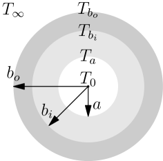
Figure 1: Schematic of a DCF with temperature markings.

A schematic transverse profile of the DCF is shown in Fig.1, where we assume a cylindrical geometry for the fiber. The core, in which the signal propagates, is marked with the inner white-filled circle of radius $a$ and is doped with rare-earth ions (typically Yb). The inner-cladding, in which the pump propagates, is the region marked with the light-gray region of radius $b$. Of course, some of the propagating pump power overlaps the core region, which is responsible for pumping the core. The outer-cladding of the fiber is the region shaded in dark-gray with radius $c$, where $D=2c$ is the total outer diameter of the fiber. We also mark the temperature of the center of the fiber core as $T_{0}$, at the core-inner-cladding boundary as $T_{a}$, at the inner-outer-cladding boundary as $T_{b}$, and the outer surface of the fiber as $T_{c}$. The ambient outside temperature is identified as $T_{\infty}$.

Before, we start our analysis, we would like to present a key result obtained in this paper:

$$\delta T_{a}=\mathfrak{X}_{a}\dfrac{D}{\mathcal{D}_{a}}\Delta T.$$ (1)

Here, $\delta T_{a}=T_{0}-T_{a}$ is the temperature variation inside the core of the optical fiber, and $\Delta T=T_{c}-T_{\infty}$ is the difference between the surface temperature of the fiber and the ambient temperature. We also have:

$$\mathcal{D}_{a}=\dfrac{4\kappa_{a}}{H},$$ (2)

where $\kappa_{a}$ is the thermal conductivity of the (fused silica) glass in units of ${\rm W/(m.K)}$ and $H$ is the convective heat transfer coefficient in units of ${\rm W/(m^{2}.k)}$ (typically that of air or water). $\mathfrak{X}_{a}$ is an order one coefficient that is to be determined and depends on the geometrical and optical properties of the laser or amplifier. We note that the fiber surface cannot be feasibly hotter than a few hundred degrees Celsius, so $\Delta T\lesssim 300^{\circ}$C is generally assumed in this paper unless stated otherwise. $D/\mathcal{D}_{a}$ is proportional to the Biot number of the thermal problem, which is a dimensionless quantity used in heat transfer calculations book . The ratio $D/\mathcal{D}_{a}$ sets the scale for $\delta T_{a}$ for a given $\Delta T$–for air-cooling, $\mathcal{D}_{a}$ is nearly two orders of magnitude larger than $D$, while it is only an order of magnitude larger for water-cooling. As such, in water-cooled systems, the core temperature can increase to the point that the fiber changes from supporting only a single-mode to supporting multiple modes due to the thermo-optic effect. However, for air-cooled DCFs with $\Delta T\lesssim 300^{\circ}$C, the core temperature rises only in the range of $0-5^{\circ}$C relative to the inner-cladding, so the thermo-optic effect is less pronounced and single-mode to multimode transition may not happen.

In the following, we will present the problem in the most general terms, while providing specific examples to illuminate the main points. In Section II, we will formulate the problem and derive the relevant equations and results. In Section III, we will apply our formalism to a few specific examples of fibers commonly used in laser and amplifier systems and examine our general conclusions using specific numerical examples. In Section IV, we will summarize and conclude. Appendices A and B provide further information about the assumptions used in deriving the analytical expressions. In Appendix C, we summarize the equations that are most useful for direct comparison with experiments.

II Formulation

In this paper, we will refer to the pump laser as the “pump”, and to the generated laser (in a laser design) or the amplified laser (in an amplifier design) as the “signal”. We present our arguments and observations in as general a form as possible without resorting to unnecessary numerical analysis in specific designs. We assume that the pump propagates only in the inner-cladding (and the core) and has a uniform intensity of $I_{p}$, which can also be a function of $z$. $P_{p}=\pi b^{2}I_{p}$ is the total pump power. This assumption is usually valid if the pump laser is sufficiently scrambled to maintain its uniformity in the transverse plane. We also define the pump overlap factor with the core as $\Gamma:=a^{2}/b^{2}$. In some DCF designs, the circular symmetry of the inner-cladding is broken to help maintain the transverse uniformity of the pump intensity along the fiber. These technicalities do not affects our general conclusions. Both the signal intensity (nearly Gaussian) and power are assumed to generally depend on the longitudinal coordinate, $z$, along the fiber. We assume that the fiber temperature is constant in time; therefore, the steady state heat equation can be used to determine the temperature distribution, $T(x,y,z)$:

$$\nabla\cdot(\kappa\nabla T)+q=0,$$ (3)

where the heat source density $q(x,y,z)$ is the thermal energy deposited per second at the location $(x,y,z)$ inside the fiber and is in units of ${\rm W/m}^{3}$ and $\kappa(x,y,z)$ is the local thermal conductivity book . Equation 3, in general, can only be solved numerically. Here, we make another simplifying assumption that the temperature gradient in the $z$-direction varies very slowly with $z$ ($\partial^{2}_{z}T\approx 0$). We will discuss the validity of this assumption later in Appendix A. Therefore, considering the cylindrical symmetry of the problem and ignoring the $\partial^{2}_{z}T$ term in Eq. 3, we arrive at the following differential equation:

$$\kappa\dfrac{\partial^{2}T}{\partial\rho^{2}}+\left(\dfrac{\kappa}{\rho}+\dfrac{\partial\kappa}{\partial\rho}\right)\dfrac{\partial T}{\partial\rho}+q=0,$$ (4)

where $\rho$ is the radial coordinate. Both $T$ and $q$ are in general functions of $z$ as well as $\rho$; however, in the following discussion, we drop their explicit $z$-dependence when writing the equations for simplicity, but their $z$-dependence is always implicitly assumed (see Appendix A). Because of the geometry of the fiber in Fig. 1, $\kappa(\rho)$ is piece-wise constant; therefore, the term proportional $\partial_{\rho}\kappa$ vanishes in each segment. Moreover, we assume that $q$ is piece-wise constant (this assumption is justified in Appendix B); therefore, the general solution to the second-order ordinary differential equation 4 in each radial segment of the fiber is given by:

$$T(\rho)={\mathcal{C}}_{1}+{\mathcal{C}}_{2}\log(\rho^{2})-\dfrac{q}{4\kappa}\rho^{2},$$ (5)

where ${\mathcal{C}}_{1}$ and ${\mathcal{C}}_{2}$ are constants of integration.

In subsection IIII.1, we summarize the definitions of the main parameters used in this paper for the temperature profiles, and in subsection IIII.2, we present the solutions that provide the temperature distributions inside the optical fiber. In subsection IIII.3, we will present and justify the values of the thermal parameters used in the paper, and in subsection IIII.4, we will elaborate on the order-one scalar coefficients that appear in equations similar to Eq. 1.

II.1 Definition of the parameters

The following parameters will be used in the solutions of Eq. 4:

• $q_{a}$ is the uniform heat density inside the core ($0\leq\rho\leq a$) due to the quantum defect, as well as the parasitic absorption of the signal and the pump.

• $q_{b}$ is the uniform heat density inside the inner-cladding ($a<\rho\leq b$) due to the parasitic absorption of the pump.

• No heat is generated in the outer-cladding region ($b<\rho\leq c$) in which no signal or pump propagates.

• $\kappa_{a}$, $\kappa_{b}$, and $\kappa_{c}$ are the thermal conductivities in the core, inner-cladding, and outer-cladding regions. Their values are assumed to be uniform in each region.

• The thermal characteristic length scales in each radial fiber segment is defined as $\mathcal{D}_{i}=4\kappa_{i}/H$, where $i=a,b,c$.

• The total linear heat density generated in the core is given by $Q_{a}=q_{a}\pi a^{2}$. Similarity, the total linear heat density generated in the inner-cladding is given by $Q_{b}=q_{b}\pi(b^{2}-a^{2})$. We also define $Q_{p}=q_{b}\pi b^{2}$, which represents the total generated linear heat density due to the parasitic absorption of the pump.

• We define the following temperatures based on $T(\rho)$: $T_{0}=T(0)$, $T_{a}=T(a)$, $T_{b}=T(b)$, $T_{c}=T(c)$, and $T_{\infty}$ as the ambient outside temperature. We also define the following temperature variation parameters: $\delta T_{a}=T_{0}-T_{a}$, $\delta T_{b}=T_{a}-T_{b}$, $\delta T_{c}=T_{b}-T_{c}$, and $\Delta T=T_{c}-T_{\infty}$.

• We use the following geometrical parameters: $\Gamma=a^{2}/b^{2}$, $\eta=\ln(c^{2}/b^{2})$, and $D=2c$.

II.2 Solution of the temperature equation

In the core, the temperature must be finite everywhere including at $\rho=0$; therefore, ${\mathcal{C}}_{2}$ from Eq. 5 must vanish in the core. Moreover, the temperature and the radial heat flux must be continuous at each layer. We remind that the radial heat flux is given by $-\kappa\partial_{\rho}T(\rho)$, where $\kappa$ is the relevant thermal conductivity in each region. The result is the following temperature profile inside the fiber at each layer:

$$T_{0}-T(\rho)=\dfrac{q_{a}\,\rho^{2}}{4\kappa_{a}},\ \ 0\leq\rho\leq a,$$ (6)

$$T_{a}-T(\rho)=\dfrac{(q_{a}-q_{b})a^{2}}{4\kappa_{b}}\ln(\dfrac{\rho^{2}}{a^{2}})+\dfrac{q_{b}(\rho^{2}-a^{2})}{4\kappa_{b}},\ \ a<\rho\leq b,$$

$$T_{b}-T(\rho)=\dfrac{q_{a}\,a^{2}+q_{b}(b^{2}-a^{2})}{4\kappa_{c}}\ln(\dfrac{\rho^{2}}{b^{2}}),\ \ b<\rho\leq c.$$

The temperature variations can be obtained as

$$(4\pi\kappa_{a})\delta T_{a}=Q_{a},$$ (7a)

$$(4\pi\kappa_{b})\delta T_{b}=(Q_{a}+Q_{b}-Q_{p})(-\ln\Gamma)+Q_{b},$$ (7b)

$$(4\pi\kappa_{c})\delta T_{c}=(Q_{a}+Q_{b})\eta.$$ (7c)

We assume convective boundary condition for the outer surface of the fiber:

$$-\kappa_{c}\dfrac{\partial T(\rho)}{\partial\rho}\Big{|}_{c}=H(T_{c}-T_{\infty}).$$ (8)

Therefore, the temperature difference between the fiber surface $T_{c}$ and ambient outside temperature $T_{\infty}$ is given by

$$\Delta T=T_{c}-T_{\infty}=\dfrac{Q_{a}+Q_{b}}{2\pi c\,H}.$$ (9)

We are now ready to simplify the previous equations and the following two relationship will be useful in the process:

$$Q_{b}=(1-\Gamma)Q_{p},\qquad Q_{a}=(\Gamma+\gamma)Q_{p}.$$ (10)

The meaning of the coefficient $\gamma$ will become clear shortly (in subsection IIII.4), but for now, Eq. 10 can be used as the definition of $\gamma$. After a few lines of algebra, we arrive at:

$$\dfrac{\delta T_{a}}{\Delta T} =\Big{[}\dfrac{\Gamma+\gamma}{1+\gamma}\Big{]}\,\dfrac{D}{\mathcal{D}_{a}},$$ (11a)

$$\dfrac{\delta T_{b}}{\Delta T} =\Big{[}\dfrac{1-\Gamma}{1+\gamma}+\dfrac{\gamma}{1+\gamma}(-\ln\Gamma)\Big{]}\,\dfrac{D}{\mathcal{D}_{b}},$$ (11b)

$$\dfrac{\delta T_{c}}{\Delta T} =\eta\,\dfrac{D}{\mathcal{D}_{c}}.$$ (11c)

Equations 11a, 11b, and  11c are the main results of this paper and will be analyzed in detail in the following discussions. Note that the total temperature change from the center of the core to the surface of the fiber is given by $\delta T_{a}+\delta T_{b}+\delta T_{c}$.

II.3 Relevant thermal parameters

In this subsection, we present the values of the relevant thermal parameters that will be used in the rest of this paper. The core and the inner-cladding of a typical DCF in fiber laser applications are made from fused silica. For both of these regions, we assume a uniform thermal conductivity across the fiber because the light doping of various elements in the core and inner-cladding do not change the value of $\kappa$ in the host glass, substantially. For fused silica at room temperature, we have $\kappa=1.38\,{\rm W/(m.K)}$ Heraeus , which is the value we will use in the subsequent analysis. However, the value of $\kappa$ increases with temperature and can reach $\approx 1.65\,{\rm W/(m.K)}$ at $320^{\circ}$C Stabler . For the outer-cladding, low-index Acrylate and Polyimide polymers are commonly used among many other polymers. While Acrylate can reliably withstand temperatures as high as $120^{\circ}$C, Polyimide coating is preferred for high power applications because it remains reliable to as high as $300^{\circ}$C in continuous operation Huang . For Polyimide, we use $\kappa\approx 0.276\,{\rm W/(m.K)}$ matweb .

The value of the convective heat transfer coefficient $H$ depends on the choice of fluid and its speed. We use $H\approx 92\,{\rm W/(m^{2}.K)}$ for a high-speed-air-fan-cooled fiber and $H\approx 920\,{\rm W/(m^{2}.K)}$ for a moderate-flow-speed-water-cooled fiber HeatTransfer .

Table 1: The thermal characteristic length scale defined as $\mathcal{D}_{i}=4\kappa_{i}/H$ for the choices of material and convection fluid. The subscript $sa$ stands for “silica” material and “air” cooling and so on.

	silica:        $\kappa=1.38\,{\rm W/(m.K)}$	Polyimide:     $\kappa=0.276\,{\rm W/(m.K)}$
forced-air-cooling $H\approx 92\,{\rm W/(m^{2}.K)}$	$\mathcal{D}_{sa}=6\,{\rm cm}$	$\mathcal{D}_{pa}=1.2\,{\rm cm}$
forced-water-cooling $H\approx 920\,{\rm W/(m^{2}.K)}$	$\mathcal{D}_{sw}=6\,{\rm mm}$	$\mathcal{D}_{pw}=1.2\,{\rm mm}$

It is clear that $\mathcal{D}_{a}$ and $\mathcal{D}_{b}$ can take the value of $\mathcal{D}_{sa}$ or $\mathcal{D}_{sw}$ depending on the choice of the cooling fluid, while $\mathcal{D}_{b}$ can take the value of $\mathcal{D}_{pa}$ or $\mathcal{D}_{pw}$. These thermal characteristic length scales must be compared with the outer diameter of the fiber as they appear in the form of a ratio in Eqs. 11a, 11b, and  11c. The outer diameter of the fiber $D$ (including the polymer coating) typically ranges from $\approx 250\,\mu{\rm m}$ to $\approx 500\,\mu{\rm m}$, so $D/\mathcal{D}_{pw}$ ranges from 2.5 to 5, $D/\mathcal{D}_{pa}$ ranges from 25 to 50, $D/\mathcal{D}_{sw}$ ranges from 12 to 25, $D/\mathcal{D}_{sa}$ ranges from 120 to 500. These ratios affect the values of temperature variations in Eqs. 11a, 11b, and  11c.

II.4 Scalar coefficients

In this subsection, we examine the scalar coefficients that appear in Eqs. 11a, 11b, and  11c, behind the ratio of the length scales $D/\mathcal{D}_{i}$:

$$\mathfrak{X}_{a} =\dfrac{\Gamma+\gamma}{1+\gamma},$$ (12a)

$$\mathfrak{X}_{b} =\dfrac{1-\Gamma}{1+\gamma}+\dfrac{\gamma}{1+\gamma}(-\ln\Gamma),$$ (12b)

$$\mathfrak{X}_{c} =\eta.$$ (12c)

We will argue that these coefficients are all order one scalars, so in each case $\delta T/\Delta T$ is primarily set by the ratio $D/\mathcal{D}_{i}$.

In a conventional cladding-pumped fiber laser or amplifier, the primary sources of heating are from the quantum defect in the core of the fiber and the parasitic absorption of both the signal and the pump. Based on our assumptions, the heating due to the quantum defect happens uniformly in the core with the linear heat density of $Q_{qd}$, which only contributes to $Q_{a}$. The linear heat density due to the parasitic absorption of the signal is given by $Q_{as}=\alpha_{s}P_{s}$ ($P_{s}$ is the total signal power), which only contributes to $Q_{a}$, as well. The linear heat density due to the parasitic absorption of the pump is given by $Q_{ap}=\alpha_{p}P_{p}$, a fraction of which, $\Gamma Q_{ap}$, contributes to $Q_{a}$ and the rest, $(1-\Gamma)Q_{ap}$, is deposited in the inner-cladding and contributes to $Q_{b}$. Here, $\alpha_{s}$ and and $\alpha_{p}$ are the parasitic absorption coefficients of the signal and the pump, respectively. Using these definitions, we obtain:

$$Q_{a}=Q_{qd}+Q_{as}+\Gamma Q_{ap},\qquad Q_{b}=(1-\Gamma)Q_{ap}.$$ (13)

Using Eq. 10 and the definitions presented in Eq. 13, it can be shown that

$$\gamma=\dfrac{Q_{qd}+Q_{as}}{Q_{ap}}.$$ (14)

Equation 14 makes the meaning of the parameter $\gamma$ more clear: $\gamma$ is the ratio of the sum of the quantum defect linear heat density and the signal parasitic absorption, both of which are deposited in the core, to the total parasitic heat generation in the fiber due to the pump. Note that $\gamma$ appears in Eqs. 12a, 12b, and 12c in the form of $1/(1+\gamma)$ and $\gamma/(1+\gamma)$, both of which are always between 0 and 1, i.e., $0\leq 1/(1+\gamma)\leq 1$ and $0\leq\gamma/(1+\gamma)\leq 1$ for $0\leq\gamma<\infty$; therefore, their finite values (bounded from above) set their contribution levels to $\mathfrak{X}_{a}$ and $\mathfrak{X}_{b}$.

From these arguments, we find that depending on the relative size of the contributions from $Q_{qd}$, $Q_{as}$, and $Q_{ap}$, which set the value of $\gamma$, we have the following acceptable ranges for the scalar coefficients:

$$\Gamma<\mathfrak{X}_{a}<1,\qquad 1-\Gamma<\mathfrak{X}_{b}<(-\ln\Gamma),\qquad\mathfrak{X}_{c}=\eta.$$ (15)

The upper limit in each case is obtained for $\gamma\gg 1$, which is usually the case for conventional fiber lasers and amplifiers, where $Q_{qd}$ is much higher than $Q_{as}$ and $Q_{ap}$ (see Eq. 14). However, in some modern high-power fiber amplifiers where the quantum defect is lowered Li , or when the amplifier operates in a nearly radiation-balanced regime or for radiation-balanced lasers bowman2010minimizing ; bowman2016low ; mobini2018thermal ; mobiniCoreCladding , $\gamma<1$ and a value closer to the lower limit in Eq. 15 may be applicable. Note that $\mathfrak{X}_{c}=\eta$ does not deviate much from unity in conventional DCFs.

III Examples

In the following, we will explore three examples of Yb-doped optical fibers from Thorlabs Incorporated, where the relevant fiber parameters are given in Table 2. We note that in all three cases, Thorlabs Incorporated reports Acrylate polymer coating, which can only withstand temperatures up to $120^{\circ}$C. For our analysis, we will assume Polyimide coating because its temperature can go as high as $300^{\circ}$C; this choice is justified because our discussions are primarily aimed at high power laser operations. For the rest of the discussion, we assume that the fiber surface is heated to $320^{\circ}$C, so $\Delta T=300^{\circ}$C, where $T_{\infty}=20^{\circ}$C is assumed. For Acrylate polymer coating where $\Delta T\approx 100^{\circ}$C, all temperature values obtained below must be divided by a factor of three. We emphasize that Fiber1 is practically a single-cladding fiber and is not commonly used in high-power operation. However, we have included this fiber here to show that the analysis in this paper can also apply to this special case, noting that the results for this fiber are somewhat less interesting than those for Fiber2 and Fiber3, which are high-power DCFs.

Table 2: The relevant fiber parameters for Eqs. 11a, 11b, and 11c.

name	fiber ID	$2a(\mu{\rm m})$	$2b(\mu{\rm m})$	$2c(\mu{\rm m})$
Fiber1	YB1200-4/125	4	125	245
Fiber2	YB1200-10/125DC	10	125	245
Fiber3	YB1200-20/400DC	20	400	520

In Tables 3, and 4, we calculate the values of the geometrical parameters and ratios of the thermal length scale to the outer diameter of for fiber for Eqs. 11a, 11b, and 11c. In Table 5, we use the information in Eqs. 12a, 12b, and 12c to estimate the temperature variations $\delta T_{a}$, $\delta T_{b}$, and $\delta T_{c}$, in the core, inner-cladding, and outer-cladding of each fiber, respectively. The results are reported for both air-cooling and water-cooling, and for a range that depends on the value of $\gamma$ as discussed earlier. In Table 6, we use Eq. 9 to calculate the total linear heat density $Q_{a}+Q_{b}$ that must be deposited inside the optical fiber to heat the surface temperature by $\Delta T=300^{\circ}$C relative to the ambient; of course, a much larger heat deposit is needed to reach the same level of $\Delta T$ for water cooling relative to air cooling.

We next consider the temperature changes for a nominal value of $Q_{a}+Q_{b}=50\,{\rm W/m}$, which is a typical value used in modern high-power fiber amplifiers Beier . Note that in the previous analysis, we fixed $\Delta T=300^{\circ}$C, but here we allow it to vary and instead fix $Q_{a}+Q_{b}$. The corresponding temperature ranges are reported in Table 7 and they are the same for air-cooling and water-cooling, because $H$ cancels out if $\Delta T$ from Eq. 9 is used in Eqs. 11a, 11b, and 11c. The total temperature change is also reported as $\sum\delta T_{i}$, which is the quantity measured in Ref. Beier . As will be noted in section IIIIII.2, the upper limit values coming from $\gamma\gg 1$ correspond to most conventional systems for which the heat density due to quantum defect overwhelms other sources of heat. In the limit of $\gamma\gg 1$, we obtain

$$\sum\delta T_{i}=\left[\dfrac{1}{4\pi\kappa_{a}}+\dfrac{(-\ln\Gamma)}{4\pi\kappa_{b}}+\dfrac{\eta}{4\pi\kappa_{c}}\right](Q_{a}+Q_{b}).$$ (16)

To make a comparison with the results reported in Ref. Beier where $2a=25\,\mu{\rm m}$ and $2b=400\,\mu{\rm m}$, if we consider the case of $Q_{a}+Q_{b}=35\,{\rm W/m}$, we obtain $\sum\delta T_{i}=22^{\circ}$C, which is in close agreement with their direct temperature measurement. Of course, if the measured core temperature is only the average value (as is the case in Ref. Beier ), $1/4\pi\kappa_{a}$ in Eq. 16 must be replaced with $1/8\pi\kappa_{a}$ because $\int_{0}^{a}\rho^{2}\rho d\rho/(a^{2}\int_{0}^{a}\rho d\rho)=1/2$ (see Eq. 6), which results in $\sum\delta T_{i}=21^{\circ}$C.

Table 3: The values of the geometrical parameters.

	$\Gamma$	$-\ln\Gamma$	$\eta$
Fiber1	0.0010	6.88	1.35
Fiber2	0.0064	5.05	1.35
Fiber3	0.0025	5.99	0.525

Table 4: The ratio of the thermal length scale to the outer diameter.

	$\mathcal{D}_{sa}/D$	$\mathcal{D}_{sw}/D$	$\mathcal{D}_{pa}/D$	$\mathcal{D}_{pw}/D$
Fiber1	123	12.2	24.5	2.45
Fiber2	123	12.2	24.5	2.45
Fiber3	57.7	5.77	11.5	1.15

Table 5: Temperature variation parameter ranges in ^∘C if $\Delta T=300^{\circ}$C.

	air-cooling			water-cooling
	$\delta T_{a}$	$\delta T_{b}$	$\delta T_{c}$	$\delta T_{a}$	$\delta T_{b}$	$\delta T_{c}$
Fiber1	0.003-2.5	2.5-17	17	0.025-25	25-169	165
Fiber2	0.016-2.5	2.4-12	17	0.16-25	24-124	165
Fiber3	0.013-5.2	5.2-31	14	0.13-52	52-312	136

Table 6: The total linear heat density $Q_{a}+Q_{b}$ needed to raise the surface temperature of the fiber relative to the ambient by $\Delta T=300^{\circ}$C.

	air-cooling (W/m)	water-cooling (W/m)
Fiber1	43	425
Fiber2	43	425
Fiber3	90	902

Table 7: Temperature variation parameter ranges in ^∘C if total linear heat density is $Q_{a}+Q_{b}=50\,{\rm W/m}$. $\delta T_{a}$, $\delta T_{b}$, and $\delta T_{c}$ are the same for both air-cooling and water cooling. We also define $\sum\delta T_{i}=\delta T_{a}+\delta T_{b}+\delta T_{c}$, which is the total temperature change inside the fiber. $\Delta T_{ac}$ is the surface temperature relative to the ambient for air-cooling and $\Delta T_{aw}$ is for water cooling.

	$\delta T_{a}$	$\delta T_{b}$	$\delta T_{c}$	$\sum\delta T_{i}$	$\Delta T_{ac}$	$\Delta T_{wc}$
Fiber1	0.003-2.9	2.9-20	19	22-42	353	35.3
Fiber2	0.019-2.9	2.9-15	19	22-37	353	35.3
Fiber3	0.007-2.9	2.9-17	8	11-28	166	16.6

III.1 Can the temperature rise result in multimode operation?

The results presented so far focus mainly on the transverse temperature variations in fused silica optical fibers. In practice, the principal optical quantity of interest is the induced change in the refractive index due to the temperature change. The change in the refractive index is related to the change in the temperature by the thermo-optic coefficient, $dn/dT$. For fused silica, the thermo-optic coefficient is reported at 546 nm to be $11.3\times 10^{-6}\,{\rm K}^{-1}$ Rocha , and does not vary substantially with the wavelength. The V-number of a step-index optical fiber for a small core-cladding index contrast of $\Delta$ is $V\approx 2\pi a\sqrt{2n\Delta}/\lambda$, where $a$ is the core radius, $n\approx 1.5$ is the average refractive index, and $\lambda$ is the optical wavelength. The single-mode cut-off is at $V\approx 2.405$. If a temperature rise results in a substantial change in the value of $\Delta$, it can turn a single-mode fiber to multimode. Using the definition of the V-number, we can show that $\delta V/V=\delta\Delta/(2\Delta)$, where $\delta\Delta$ is the change in the core-cladding index difference. For a single-mode large-core fiber of $V\approx 2.3$ with a $30\,\mu{\rm m}$ core diameter at $\lambda\approx 1\,\mu{\rm m}$, $\Delta\approx 2\times 10^{-4}$. Assuming a maximum tolerable change in the V-number of 20%, the maximum acceptable $\delta\Delta$ is $8\times 10^{-5}$. We can approximate $\delta\Delta\approx(dn/dT)\delta T_{a}$, given that $\delta T_{a}$ sets the scale for the core-cladding temperature variation, resulting in a maximum acceptable value of $\delta T_{a}\approx 8^{\circ}$C. Of course, the temperature profile in the core is not of a top-hat form and decreases quadratically, so this analysis slightly underestimates the $\delta T_{a}$ required for the fiber core to support multiple modes.

The results presented for the value of $\delta T_{a}$ in Table 5 indicate that for air-cooling and $\Delta T=300^{\circ}$C, the temperature variation range in the core is quite small and the fiber is unlikely to transition from single-mode to multimode. However, in a water-cooled system, the value of $\delta T_{a}$ can be as high as $25^{\circ}$C for Fiber1 and Fiber2 and as high as $50^{\circ}$C for Fiber3, which can clearly result in a multimode core in the high-heat and $\gamma\gg 1$ (conventional) operation.

III.2 Estimation of the $\gamma$ parameter

We already noted in Eq. 14 that $\gamma$ is the ratio of the sum of the quantum defect linear heat density and the signal parasitic absorption to the total parasitic heat generation in the fiber due to the pump. We can obtain an estimate of this parameter if we assume for example an amplifier set-up in the forward pumping configuration, where at the input the signal power can be neglected compared with the pump power. In this case, $Q_{qd}\approx\alpha_{r}P_{p}\delta\lambda/\lambda_{s}$ (see Appendix B for the derivation). $\alpha_{r}$ is the resonant pump absorption coefficient and is given by $N_{t}\sigma^{a}_{p}\Gamma$, where $N_{t}$ is total Yb ion dopant density and $\sigma^{a}_{p}$ is the absorption cross section of the pump. $\delta\lambda=\lambda_{s}-\lambda_{p}$ is the difference between the wavelengths of the signal and the pump. Noting that $Q_{ap}=\alpha_{p}P_{p}$ and $Q_{as}\approx 0$, so we have

$$\gamma\approx\dfrac{\alpha_{r}}{\alpha_{p}}\times\dfrac{\delta\lambda}{\lambda_{s}}.$$ (17)

This is an interesting result and gives an estimate on the value of $\gamma$, independent of the pump power. For our analysis, we consider a nominal value of $\alpha_{p}\approx 15\,{\rm dB/km}$, which is reasonable for conventional high-power fiber lasers. For pumping at the peak absorption wavelength $\lambda_{p}=976\,{\rm nm}$, the nominal values of $\alpha_{r}$ for Fiber1, Fiber2, and Fiber3 are $1200\,{\rm dB/m}$, $7.4\,{\rm dB/m}$, and $3\,{\rm dB/m}$, respectively. For $\lambda_{s}\approx 1064\,{\rm nm}$, $\delta\lambda/\lambda_{s}\approx 0.1$, so the corresponding values of $\gamma$ are approximately $8000$, $50$, and $20$, respectively. If the same fibers are pumped at $\lambda_{p}=920\,{\rm nm}$, the measured values of $\alpha_{r}$ for Fiber1, Fiber2, and Fiber3 would be $280\,{\rm dB/m}$, $1.7\,{\rm dB/m}$, and $0.7\,{\rm dB/m}$, respectively. Given that $\delta\lambda/\lambda_{s}\approx 0.14$, the corresponding values of $\gamma$ are approximately $2520$, $15.3$, and $6.3$, respectively.

However, for a low quantum defect fiber amplifier Li pumped at $\lambda_{p}=1018\,{\rm nm}$, the nominal value of $\alpha_{r}$ would be 10 times smaller than that for $\lambda_{p}=920\,{\rm nm}$ due to a smaller absorption cross section of the pump. In this case, $\delta\lambda/\lambda_{s}\approx 0.05$, and the corresponding values of $\gamma$ are approximately $93$, $0.57$, and $0.23$, respectively. Note the small value of $\gamma$ for Fiber3, which is often used in high-power operation (unlike Fiber1, which is a single-cladding fiber). The value of $\gamma$ can become even lower in the nearly radiation-balanced regime bowman2010minimizing ; bowman2016low ; mobini2018thermal ; mobiniCoreCladding .

IV Summary and Conclusion

The analytical expressions for temperature variations are simple and can be used for quick estimation of the temperature distributions inside the optical fiber. The inclusion of the heat generation in the cladding is essential for modern high-power fiber lasers and amplifiers, where the quantum defect is lowered, or when the amplifier operates in a nearly radiation-balanced regime, or for radiation-balanced lasers. In all these cases, the heat generated due to the parasitic absorption of the high-power pump in the inner-cladding can be considerable and must be included in the analysis. The analytical expressions can be used for a wide range of conventional DCF-based systems. A single parameter $0\ll\gamma<\infty$ allows one to interpolate between the case where the quantum defect heating is dominant to when the parasitic absorption heating is comparable in size or is the dominant source of heating.

For the numerical analysis of the analytical expressions, we consider the maximum tolerable surface temperature of the fiber relative to the ambient to be $\Delta T=300^{\circ}$C to protect the Polyimide coating that is the polymer of choice in high-temperature operation. Our results show that for air-cooled DCFs with $\Delta T\lesssim 300^{\circ}$C, the core temperature rises only in the range of $0-5^{\circ}$C relative to the inner-cladding; however, for water-cooled DCFs, the core temperature can be higher than the inner-cladding by as much as $50^{\circ}$C, potentially resulting in a change from the single-mode core to the multimode cre due to the thermo-optic effect.

Last but not least, in Appendix C, we summarize the equations that are most useful for direct comparison with experiments.

Appendix A: Longitudinal variation of the temperature

In this Appendix, we would like to justify the absence of the $\partial^{2}_{z}T$ term in our analysis based on Eq. 4. Let’s consider a situation where $q$ is Eq. 3 can be expressed as $q(\rho,z)=\tilde{q}(\rho)\,f(z)$. This separable form, while very convenient in our analysis, can be fully justified if only one of the heating sources, $Q_{qd}$, $Q_{as}$, or $Q_{ap}$, is the dominant one. However, our discussion captures the essence of why the $\partial^{2}_{z}T$ term can be ignored, regardless.

The analysis presented in this paper means that the temperature profile has a $\rho$-dependence subject to the form of Eq. 4 with $\tilde{q}(\rho)$ as the heat source, and a $z$-dependence of the form $f(z)$. In other words, $T(\rho,z)\approx\widetilde{T}(\rho)f(z)$, where

$$\frac{\partial^{2}\widetilde{T}(\rho)}{\partial\rho^{2}}+\frac{1}{\rho}\frac{\partial\widetilde{T}(\rho)}{\partial\rho}+\dfrac{\tilde{q}(\rho)}{\kappa}=0.$$ (18)

Without making any approximations, the full form of the temperature profile can be expressed as

$$T(\rho,z)=\widetilde{T}(\rho)f(z)+\tau(\rho,z),$$ (19)

where $\tau(\rho,z)$ should be negligible if our approximations hold. In other words, the size of $\tau(\rho,z)$ characterizes the relative importance of keeping the $\partial^{2}_{z}T$ term in Eq. 3.

If we substitute $T(\rho,z)$ from Eq. 19 in Eq. 3, while considering Eq. 18, we arrive at

$$\nabla^{2}\,\tau(\rho,z)+\widetilde{T}(\rho)\,\partial_{z}^{2}f(z)=0.$$ (20)

In Eq. 20, the term $\partial^{2}_{z}f(z)$ can be approximated into the form of $f(z)/\widetilde{L}$, where $\widetilde{L}$ is a length-scale on the order of the full length of the optical fiber. This can be understood for example if $f(z)\sim\exp(-\widetilde{\alpha}\,z)$, where $\widetilde{\alpha}$ can be, e.g., the absorption coefficient of the pump, and the pump power is almost entirely absorbed over the full length of the fiber laser. If the pump power is not fully absorbed, then $\widetilde{L}$ can be even larger than the length of the optical fiber. Next, looking at Eq. 6 reveals that the radial temperature profile of the fiber has, generally speaking, the form of $\widetilde{T}(\rho)\sim\tilde{\rho}^{2}\,\tilde{q}(\rho)/4\kappa$, where $\tilde{\rho}^{2}$ is a length scale comparable to the radius of the fiber. Therefore, we can approximate Eq. 20 as

$$\nabla^{2}\tau(\rho,z)+\dfrac{\tilde{\rho}^{2}}{\widetilde{L}^{2}}\dfrac{\tilde{q}(\rho)f(z)}{\kappa}=0.$$ (21)

Comparing Eq. 21 with Eq. 18, it can be readily observed that

$$\tau(\rho,z)\sim\dfrac{\tilde{\rho}^{2}}{\widetilde{L}^{2}}\widetilde{T}(\rho)f(z),$$ (22)

therefore, $\tau(\rho,z)$ is smaller than $\widetilde{T}(\rho)f(z)$ by the factor of $\tilde{\rho}^{2}/\widetilde{L}^{2}$, which is usually 4 orders of magnitude or more.

In summary, $\partial^{2}_{z}T$ term can be ignored unless longitudinal variations in heat deposit in the fiber occur at scales comparable to the fiber diameter, which is hardly conceivable in steady-state.

Appendix B: Validity of Top hat Assumption

In the main text of the paper, we assume that the heat density $q$ is piece-wise constant, which serves as a convenient assumption to simplify the analytical solution of the steady state heat equation. In reality, the signal intensity in a single-mode fiber core follows a nearly Gaussian profile, so the piece-wise constant assumption is not strictly true in the core of the fiber. However, it is important to asses the accuracy of this assumption, because the heating profile in the core is the main underlying factor in transitioning from the single-mode to multimode operation due to the thermo-optic effect.

In the following analysis, we borrow from the formalism presented by Bowman in Ref. bowman2015 , primarily developed to analyze the heat generation in low quantum defect lasers. The interested reader may consult that paper for further details.

The total heat source density $q(x,y,z)$, i.e. the thermal energy deposited per second at the location $(x,y,z)$ inside the fiber in units of ${\rm W/m}^{3}$ is given by $q=q_{qd}+q_{fl}+q_{ap}+q_{as}$:

$$q_{qd} =\left(\dfrac{N_{t}hc}{\tau_{r}}\right)\dfrac{\lambda_{s}\beta_{p}i_{p}+\lambda_{p}\beta_{s}i_{s}+(\lambda_{s}-\lambda_{p})(\beta_{p}-\beta_{s})i_{p}i_{s}}{\lambda_{s}\lambda_{p}(1+i_{p}+i_{s})},$$ (23a)

$$q_{fl} =-\left(\dfrac{N_{t}hc}{\tau_{r}}\right)\dfrac{\beta_{p}i_{p}+\beta_{s}i_{s}}{\lambda_{f}(1+i_{p}+i_{s})},$$ (23b)

$$q_{ap} =\alpha_{p}I_{p},\qquad q_{as}=\alpha_{s}I_{s}.$$ (23c)

$q_{qd}$ is the contribution due to the quantum defect and $q_{fl}$ is the contribution from fluorescence where the negative sign indicates that it is a heat drain. $q_{ap}$ and $q_{as}$ are contributions due to the parasitic absorption of the pump and the signal, respectively. $N_{t}$ is total Yb ion dopant density, $h$ is the Planck’s constant, $c$ is the speed of light, and $\tau_{r}$ is the upper-level lifetime of Yb ions doped in silica, which can be almost equal to its total lifetime Mobini2019 . $\sigma^{a}_{p}$ and $\sigma^{a}_{s}$ are the absorption cross sections of the pump and signal, while $\sigma^{e}_{p}$ and $\sigma^{e}_{s}$ are the emission cross sections of the pump and signal, respectively. We also define:

$$\beta_{p}=\dfrac{\sigma^{a}_{p}}{\sigma^{a}_{p}+\sigma^{e}_{p}},\quad\beta_{s}=\dfrac{\sigma^{a}_{s}}{\sigma^{a}_{s}+\sigma^{e}_{s}}.$$ (24)

$I_{p}$ and $I_{s}$ are the local pump and signal intensities, while $i_{p}$ and $i_{s}$ are the same quantities normalized by their corresponding saturation values. We have

$$i_{p}=\dfrac{I_{p}}{I_{p}^{\rm sat}},\qquad I_{p}^{\rm sat}=\dfrac{hc\beta_{p}}{\lambda_{p}\tau_{r}\sigma^{a}_{p}},$$ (25a)

$$i_{s}=\dfrac{I_{s}}{I_{s}^{\rm sat}},\qquad I_{s}^{\rm sat}=\dfrac{hc\beta_{s}}{\lambda_{s}\tau_{r}\sigma^{a}_{s}}.$$ (25b)

$\lambda_{f}$ is the mean fluorescence wavelength and is defined in Ref. bowman2015 .

Unless the fiber laser or amplifier system is especially tuned to operate in a nearly radiation-balanced regime bowman2010minimizing ; bowman2016low ; mobini2018thermal ; mobiniCoreCladding , the contribution from $q_{fl}$ can be ignored. In a conventional DCF laser or amplifier where the signal and pump powers are nearly of the same order of magnitude, the signal intensity is substantially higher than the pump intensity because the signal propagates in a much smaller area in the core. It can be readily seen that the limit of $1\ll i_{p}\ll i_{s}$ commonly applies. In this limit, we have

$$q_{qd}\approx\left(\dfrac{N_{t}hc}{\tau_{r}}\right)\dfrac{(\lambda_{s}-\lambda_{p})\beta_{p}i_{p}}{\lambda_{s}\lambda_{p}}=N_{t}\sigma^{a}_{p}I_{p}\left(\dfrac{\lambda_{s}-\lambda_{p}}{\lambda_{s}}\right),$$ (26)

which is the formula that was presented earlier in section IIIIII.2. Here, we have taken into account that $\beta_{p}\gg\beta_{s}$. Equation 26 clearly shows that the heat due the quantum defect follows a top-hat profile in high-power DCF lasers and amplifiers, because it is proportional to $i_{p}$ rather than $i_{s}$ in the limit of $i_{p}\ll i_{s}$. Note that this top-hat form is enforced by the signal saturation effect in the core. Also, in the inner-cladding where $i_{s}=0$, the heat density is also uniform as assumed in this paper.

Near the tail of the signal at the core-inner-cladding boundary, $i_{p}\ll i_{s}$ may no longer be valid, so that will present a deviation form the top-hat assumption for the heat generation. Also, if the input signal power is low in an amplifier set-up, $i_{p}\ll i_{s}$ may not apply near the input and the heat profile in the core may shape somewhere between a Gaussian and a top-hat depending on the specifics of the problem. Moreover, unlike $q_{ap}$ which is of the top-hat form, $q_{as}$ follows the near-Gaussian profile of the signal. If the contribution of $q_{as}$ is considerable, the top-hat assumption must be revisited. The contribution from $q_{fl}$ must also be included in radiation-balanced lasers and amplifiers bowman2010minimizing ; bowman2016low ; mobini2018thermal ; mobiniCoreCladding . However, in all these cases, the piece-wise constant assumption for $q(\rho)$ in the radial coordinate should give a reasonably accurate assessment of the temperature profile in the core if all the sources of heating are considered. Of course, the cladding temperature profiles are not affected and the piece-wise assumption for the inner-cladding always holds.

Appendix C: Most useful formulas

In this Appendix, we summarize the equations that are most useful for direct comparison with experiments. In this Appendix, we only consider the case where the heat density due to quantum defect in the core ($Q_{qd}$) overwhelms other sources of heat, as in the case in conventional fiber lasers and amplifiers. The more general case is treated in detail in the main text of the paper. The most relevant equations are:

$$\Delta T =\dfrac{Q_{qd}}{2\pi c\,H},$$ (27a)

$$\delta T_{a} =\dfrac{Q_{qd}}{4\pi\kappa_{a}},$$ (27b)

$$\delta T_{b} =\ln\left(\dfrac{b^{2}}{a^{2}}\right)\dfrac{Q_{qd}}{4\pi\kappa_{b}},$$ (27c)

$$\delta T_{c} =\ln\left(\dfrac{c^{2}}{b^{2}}\right)\dfrac{Q_{qd}}{4\pi\kappa_{c}}.$$ (27d)

For example, for $Q_{qd}=40\,{\rm W/m}$, outer diameter of $2c=245\,\mu{\rm m}$, core and inner-cladding of glass with $\kappa_{a}=\kappa_{b}=1.38\,{\rm W/(m.K)}$, outer-cladding of polymer with $\kappa_{c}=0.276\,{\rm W/(m.K)}$, and $H\approx 920\,{\rm W/(m^{2}.K)}$ for a moderate-flow-speed-water-cooled fiber, we obtain:

$$\Delta T=56^{\circ}{\rm C},\ \delta T_{a}=3.46^{\circ}{\rm C},\ \delta T_{b}=11.7^{\circ}{\rm C},\ \delta T_{c}=15.5^{\circ}{\rm C}.$$

Funding Information

This material is based upon work supported by the Air Force Office of Scientific Research under award number FA9550-16-1-0362 titled Multidisciplinary Approaches to Radiation Balanced Lasers (MARBLE).

Disclosures

The author declares no conflicts of interest.

References

- (1) L. Zenteno, “High-power double-clad fiber lasers,” J. Light. Technol. 11, 1435–1446 (1993).
- (2) D. J. Richardson, J. Nilsson, and W. A. Clarkson, “High power fiber lasers: current status and future perspectives [invited],” J. Opt. Soc. Am. B 27, B63–B92 (2010).
- (3) M. N. Zervas and C. A. Codemard, “High power fiber lasers: a review,” IEEE J. Sel. Top. Quantum Electron. 20, 219–241 (2014).
- (4) F. Beier, C. Hupel, S. Kuhn, S. Hein, J. Nold, F. Proske, B. Sattler, A. Liem, C. Jauregui, J. Limpert, N. Haarlammert, T. Schreiber, R. Eberhardt, and A. T ünnermann, “Single mode 4.3 kW output power from a diode-pumped Yb-doped fiber amplifier,” Opt. Express 25, 14892–14899 (2017).
- (5) Arlee V. Smith and Jesse J. Smith, “Mode instability in high power fiber amplifiers,” Opt. Express 19, 10180–10192 (2011).
- (6) B. Ward, C. Robin, and I. Dajani, “Origin of thermal modal instabilities in large mode area fiber amplifiers,” Opt. Express 20, 11407–11422 (2012).
- (7) C. Jauregui, T. Eidam, H.-J. Otto, F. Stutzki, F. Jansen, J. Limpert, and A. Tünnermann, “Temperature-induced index gratings and their impact on mode instabilities in high-power fiber laser systems,” Opt. Express 20, 440–451 (2012).
- (8) C. Jauregui, T. Eidam, H.-J. Otto, F. Stutzki, F. Jansen, J. Limpert, and A. Tünnermann, “Physical origin of mode instabilities in high-power fiber laser systems,” Opt. Express 20, 12912–12925 (2012).
- (9) V. Scarnera, F. Ghiringhelli, A. Malinowski, C. A. Codemard, M. K. Durkin, and M. N. Zervas, “Modal instabilities in high power fiber laser oscillators,” Opt. Express 27, 4386–4403 (2019).
- (10) D. C. Brown and H. J. Hoffman, “Thermal, stress, and thermo-optic effects in high average power double-clad silica fiber lasers,” IEEE J. Quantum Electron 37, 207–217 (2001).
- (11) L. Li, H. Li, T. Qiu, V. L. Temyanko, M. M. Morrell, A. Schülzgen, A. Mafi, J. V. Moloney, and N. Peyghambarian, “3-Dimensional thermal analysis and active cooling of short-length high-power fiber lasers,” Opt. Express 13, 3420–3428 (2005).
- (12) S. Hädrich, T. Schreiber, T. Pertsch, J. Limpert, T. Peschel, R. Eberhardt, and A. Tünnermann, “Thermo-optical behavior of rare-earth-doped low-NA fibers in high power operation,” Opt. Express 14, 6091-6097 (2006).
- (13) Y. Fan, B. He, J. Zhou, J. Zheng, H. Liu, Y. Wei, J. Dong, and Q. Lou, “Thermal effects in kilowatt all-fiber MOPA,” Opt. Express 19, 15162–15172 (2011).
- (14) K. R. Hansen, T. T. Alkeskjold, J. Broeng, and J. Lægsgaard, “Thermo-optical effects in high-power Ytterbium-doped fiber amplifiers,” Opt. Express 19, 23965–23980 (2011).
- (15) L. Mousavi, M. Sabaeian, and H. Nadgaran, “Numerical modelling of self-heating effects on guiding modes of high-power photonic crystal fibre lasers,” Lith. J. Phys 53, 104–111 (2013).
- (16) S. L. Mousavi and M. Sabaeian, “Thermal stress-induced depolarization loss in conventional and panda-shaped photonic crystal fiber lasers,” Braz. J. Phys 46, 481–488 (2016).
- (17) R. Li, H. Xiao, J. Leng, Z. Chen, J. Xu, J. Wu, and P. Zhou, “2240 W high-brightness 1018 nm fiber laser for tandem pump application,” Laser Physics Letters 14, 125102 (2017).
- (18) S. R. Bowman, S. P. O’Connor, S. Biswal, N. J. Condon, and A. Rosenberg, “Minimizing heat generation in solid-state lasers,” IEEE J. Quantum Electron. 46, 1076–1085 (2010).
- (19) S. R. Bowman, “Low quantum defect laser performance,” Optical Engineering 56, 011104 (2016).
- (20) E. Mobini, M. Peysokhan, B. Abaie, and A. Mafi, “Thermal modeling, heat mitigation, and radiative cooling for double-clad fiber amplifiers,” J. Opt. Soc. Am. B 35, 2484–2493 (2018).
- (21) E. Mobini, M. Peysokhan, and A. Mafi, “Heat mitigation of a core/cladding Yb-doped fiber amplifier using anti-Stokes fluorescence cooling,” J. Opt. Soc. Am. B 36, 2167–2177 (2019).
- (22) D. W. Hahn and M. N. Özisik, Heat conduction (John Wiley & Sons, 2012).
- (23) Heraeus Group, “Properties of fused silica,” https://www.heraeus.com/
- (24) C. Stabler, A. Reitz, P. Stein, B. Albert, R. Riedel, and E. Ionescu, “Thermal Properties of SiOC Glasses and Glass Ceramics at Elevated Temperatures,” Materials 11, 279 (2018).
- (25) L. Huang, R. S. Dyer, R. J. Lago, A. A. Stolov, and J. Li, “Mechanical properties of polyimide coated optical fibers at elevated temperatures,” Proc. SPIE 9702, Optical Fibers and Sensors for Medical Diagnostics and Treatment Applications XVI, 97020Y (2016).
- (26) Material Property Database, “http://www.matweb.com/”
- (27) Engineering ToolBox, “Overall heat transfer coefficient,” https://www.engineeringtoolbox.com/overall-heat-transfer-coefficient-d434.html
- (28) F. Beier, M. Plötner, B. Sattler, F. Stutzki, T. Walbaum, A. Liem, N. Haarlammert, T. Schreiber, R. Eberhardt, and A. Tünnermann, “Measuring thermal load in fiber amplifiers in the presence of transversal mode instabilities,” Opt. Lett. 42, 4311–4314 (2017).
- (29) A. C. P. Rocha, J. R. Silva, S. M. Lima, L. A. O. Nunes, and L. H. C. Andrade, “Measurements of refractive indices and thermo-optical coefficients using a white-light Michelson interferometer,” Appl. Opt. 55, 6639–6643 (2016).
- (30) S. R. Bowman, “Optimizing average power in low quantum defect lasers,” Appl. Opt. 54, F78–F84 (2015).
- (31) E. Mobini, M. Peysokhan, B. Abaie, M. P. Hehlen, and A. Mafi, “Spectroscopic Investigation of -Doped Silica Glass for Solid-State Optical Refrigeration”, Phys. Rev. Applied 11, 014066 (2019).