Synthesis of Deceptive Strategies in Reachability Games with Action Misperception

Abstract

We consider a class of two-player turn-based zero-sum games on graphs with reachability objectives, known as reachability games, where the objective of Player 1 (P1) is to reach a set of goal states, and that of Player 2 (P2) is to prevent this. In particular, we consider the case where the players have asymmetric information about each other’s action capabilities: P2 starts with an incomplete information (misperception) about P1’s action set, and updates the misperception when P1 uses an action previously unknown to P2. When P1 is made aware of P2’s misperception, the key question is whether P1 can control P2’s perception so as to deceive P2 into selecting actions to P1’s advantage? We show that there might exist a deceptive winning strategy for P1 that ensures P1’s objective is achieved with probability one from a state otherwise losing for P1, had the information being symmetric and complete. We present three key results: First, we introduce a dynamic hypergame model to capture the reachability game with evolving misperception of P2. Second, we present a fixed-point algorithm to compute the dasw region and dasw strategy. Finally, we show that dasw strategy is at least as powerful as asw strategy in the game in which P1 does not account for P2’s misperception. We illustrate our algorithm using a robot motion planning in an adversarial environment.

1 Introduction

Synthesis of winning strategies in reachability games is a central problem in reactive synthesis Pnueli and Rosner (1989), control of discrete event systems Ramadge and Wonham (1989), and robotics Fainekos et al. (2009). In a two-player reachability game, a controllable player, P1 (pronoun “she”), plays against an uncontrollable adversarial player, P2 (pronoun “he”), to reach the goal states. These games have been extensively studied in algorithmic game theory de Alfaro et al. (2007) and reactive synthesis Bloem et al. (2012). Polynomial-time algorithms are known for synthesizing sure-winning and almost-sure winning strategies, when both players have complete and symmetric information. However, the solution concepts for such games under asymmetric information have not been thoroughly studied.

Information asymmetry arises when a player has some private information that are not shared with others Rasmusen (1989). We consider the case when P1 has complete information about both players’ action capabilities, but P2 starts with an incomplete information about P1’s action capabilities. As two players interact, their information evolves. Particularly, when P1 uses an action previously unknown to P2, P2 can update his knowledge about the other’s capabilities using an inference-mechanism. In response, P2 would update his counter-strategy. We are interested in the following question: if P1 is made aware of the initial information known to P2 and his inference mechanism, can P1 find a strategy to control P2’s information in such a way that P2’s counter-strategy given his evolving information is advantageous to P1? In the context of reachability game, the question translates to: from a state that is losing for P1 in a game with symmetric information, can P1 reach his goal from the same state when the information is asymmetric? We note that a strategy of P1 that controls P2’s information to P1’s advantage is indeed deceptive Ettinger and Jehiel (2010). In this paper, we show that such a deceptive winning strategy may exist and propose an algorithm to synthesize it.

We approach the question based on the modeling and solution concepts of hypergame Bennett (1977). A hypergame allows players to play different games and further allows players to model the games that others are playing. In the literature, hypergames and Bayesian games are common models to capture game-theoretic interactions with asymmetric, incomplete information. In Bayesian games, each player uses his incomplete information to define a probability distribution over the possible types of the opponent. The distributions over types are assumed to be common knowledge. In hypergames, no such probabilistic characterizations of incomplete information is used or assumed. For action deception, P2 has incomplete information about P1’s capabilities but does not have a prior knowledge about the set of possible types of P1. Thus, we adopt the hypergame model Gharesifard and Cortés (2012) to understand action deception. In the past, hypergame model has been used to study deception Gutierrez et al. (2015); Kovach (2016). These papers mainly focus on extending the notion of Nash equilibrium to level-$k$ normal form hypergames. Gharesifard and Cortés (2014) use the notion of H-digraph to establish necessary and sufficient conditions for deceivability. An H-digraph models a hypergame as a graph with nodes representing different outcomes in a normal-form game. However, our game model is not a normal-form game, but instead a game on graph. A hypergame model based on a game on graph has been defined in Kulkarni and Fu (2019) where one player has incomplete information about the other’s task specification. However, their model assumes that the misperception of P2 remains constant, whereas in our case, the game is dynamic with both players’ evolving perception.

To synthesize deceptive strategies, we first define a dynamic hypergame on graph and then introduce an algorithm to identify the deceptive almost-sure winning region, which contains a set of states from where P1 has a deceptive strategy to ensure that the goal is reached with probability one. Our main contributions are as follows.

A Modeling Framework with Dynamic Hypergame

The dynamic hypergame on graph models (i) the evolving information of P2, and (ii) the P1’s information regarding current perception of P2.

dasw Synthesis Algorithm

We propose an algorithm to identify the dasw region and synthesize a dasw strategy. We prove that the computed dasw region is a superset of asw region, which implies that the dasw strategy is at least as powerful as the asw strategy.

2 Preliminaries

Let $\Sigma$ be a finite alphabet. A sequence of symbols $w=w_{0}w_{1}\ldots w_{n}$ with $w_{i}\in\Sigma,i=0,1,\ldots,n$ is called a finite word and $\Sigma^{\ast}$ is the set of finite words that can be generated with alphabet $\Sigma$. We denote by $\Sigma^{\omega}$, the set of $\omega$-regular words obtained by concatenating the elements in $\Sigma$ infinitely many times. Given a set $X$, let $\mathsf{Dist}(X)$ be the set of probability distributions over $X$. Given a distribution $\delta\in\mathsf{Dist}(X)$, the set $\mathsf{Supp}(\delta)=\{x\in X\mid\delta(x)>0\}$ is called the support of the distribution.

2.1 Games on Graph

Consider an interaction between two players; P1 with a reachability objective and P2 with an objective of preventing P1 from completing her task.

Definition 1 (Game on Graph).

Let the action sets of P1 and P2 be $A_{1}$ and $A_{2}$, respectively. Then, a turn-based game on graph is the tuple

$$\mathcal{G}=\langle S,{Act},T,F\rangle,$$

where

• $S=S_{1}\cup S_{2}$ is the set of states partitioned into P1’s states, $S_{1}$, and P2’s states, $S_{2}$. P1 chooses an action when $s\in S_{1}$ and P2 chooses an action when $s\in S_{2}$.

• ${Act}=A_{1}\cup A_{2}$ is set of actions for P1 and P2.

• $T:S\times{Act}\rightarrow S$ is a deterministic transition function that maps a state and an action to a successor state.

• $F\subseteq S$ is a set of final states.

A trace in the game $\mathcal{G}$ is an infinite, ordered sequence of state-action pairs $\tau=(s_{0},a_{0}),(s_{1},a_{1}),(s_{2},a_{2}),\ldots$. We write $\tau[n]=(s_{n},a_{n})$ to denote $n$-th state-action pair, and $\tau[m:n]=(s_{m},a_{m}),\ldots,(s_{n},a_{n})$ to denote a state-action pairs between $m$-th and $n$-th step, both inclusive. A run is the projection of trace onto the state-space. We denote it as the sequence $\rho=\tau\downharpoonright_{S}=s_{0}s_{1}s_{2}\ldots$. Similarly, the action-history is the projection of trace onto the action space, denoted by $\alpha=\tau\downharpoonright_{Act}=a_{0}a_{1}a_{2}\ldots$. The $k$-th element in a run (resp. action-history) is denoted by $\rho_{k}$ (resp. $\alpha_{k}$).

In this paper, we consider reachability objectives for P1. The set of states that occur in a run is given by $\mathsf{Occ}(\rho)=\{s\in S\mid\exists k\in\mathbb{N}\cdot s=\rho_{k}\}$. A run is said to be winning for P1 in the reachability objective if it satisfies $\mathsf{Occ}(\rho)\cap F\neq\emptyset$. If a run is not winning for P1, then it is winning for P2.

asw Strategy

A stochastic or randomized strategies for P1 and P2 are defined as $\pi:S_{1}\rightarrow\mathsf{Dist}(A_{1})$ and $\sigma:S_{2}\rightarrow\mathsf{Dist}(A_{2})$, respectively. Let $\Omega_{s}^{\pi,\sigma}$ be the exhaustive set of runs that result when P1 and P2 play strategies $\pi$ and $\sigma$ in a game starting at the state $s\in S$. The randomized strategies of P1 and P2 induce a Markov chain from $\mathcal{G}$–that is, a probability distribution over the set $\Omega_{s}^{\pi,\sigma}$.

Given a state $s\in S$, a randomized strategy $\pi$ is almost-sure winning for P1, if and only if for every possible randomized strategy $\sigma$ of P2, the probability is one for a run that satisfies $\mathsf{Occ}(\rho)\cap F\neq\emptyset$, given the distribution of runs induced by $(\pi,\sigma)$. A state is called an almost-sure winning state for P1, if there exists an almost-sure winning strategy for P1 from that state. The exhaustive set of almost-sure winning states for P1 is called her almost-sure winning region. The almost-sure winning region can be computed using Alg. 1 based on the Proposition 1.

Algorithm 1 Zielonka’s Algorithm

1:$\mathcal{G},F$

2:$Z_{0}=F$

3:while True do

4:     $\mathsf{Pre}_{1}(Z_{k})=\{s\in S_{1}\mid\exists a\in A_{1}\text{ s.t. }T(s,a)\in Z_{k}\}$

5:     $\mathsf{Pre}_{2}(Z_{k})=\{s\in S_{2}\mid\forall b\in A_{2}:T(s,b)\in Z_{k}\}$

6:     $Z_{k+1}=Z_{k}\cup\mathsf{Pre}_{1}(Z_{k})\cup\mathsf{Pre}_{2}(Z_{k})$

7:     if $Z_{k+1}=Z_{k}$ then

8:         End Loop

9:     end if

10:end while

11:return $Z_{k}$

Proposition 1.

(From (de Alfaro et al., 2007, Thm 3)) In a deterministic and turn-based game, the almost-sure winning region is equal to sure-winning region.

Let us introduce a running example that we shall use to explain the concepts in this paper.

Example 1.

Consider the game graph in Fig. 1. The circle states, $\{s_{1},s_{3}\}$, are P1 states and the square states, $\{s_{0},s_{2}\}$, are P2 states. The objective of P1 is to reach to the final state $s_{0}$ from the initial state $s_{2}$. P1’s action set is $A_{1}=\{a_{1},a_{2}\}$, and P2’s action set is $A_{2}=\{b_{1},b_{2}\}$.

Figure 1: An example game on graph

The asw region for P1 in the game is $\mathsf{Win}_{1}=\{s_{0},s_{1}\}$. This can intuitively be understood as follows. P1 can win from state $s_{1}$ by choosing the action $a_{1}$. However, the states $s_{2}$ and $s_{3}$ are losing for P1 because P2 has a strategy to indefinitely restrict the game within the states $s_{2},s_{3}$ by choosing the action $b_{2}$ at the state $s_{2}$.

2.2 Action Misperception and Information Asymmetry

In this paper, we make the following assumption about the reachability game, in which the P2 has asymmetric information about P1’s action capabilities.

Assumption 1.

P1 has complete information about the players’ action sets, i.e. P1 knows $A_{1}$ and $A_{2}$. P2 only knows his own action set $A_{2}$, but (mis)perceives P1’s action set to be a subset $X\subsetneq A_{1}$. Both players have complete information about the game state-space $S$, transition function $T$ and the final states $F$.

The result of Assumption 1 is that P1 and P2, in their minds, play different games to synthesize their respective strategies. We refer to these games as the perceptual games of the players. P1’s perceptual game is identical to the ground-truth game; $\mathcal{G}(A_{1})=\langle S,A_{1}\cup A_{2},T,F\rangle$, while P2’s perceptual game is a game under misperception; $\mathcal{G}(X)=\langle S,X\cup A_{2},T,F\rangle$. Let us formalize the new notation used to distinguish between the perceptual games of P1 and P2.

Notation 1.

Let $X\subseteq A_{1}$ be a subset of P1’s action set. We denote a perceptual game in which P1’s action set is $X$ by $\mathcal{G}(X)=\langle S,X\cup A_{2},T,F\rangle$. The winning regions for P1 and P2 in the game $\mathcal{G}(X)$ are denoted by $\mathsf{Win}_{1}(X)$ and $\mathsf{Win}_{2}(X)$, respectively.

Assuming P1 and P2 to be rational players, they would use the solution approach reviewed in Section 2.1 to compute their winning strategies in their respective perceptual games. That is, P1 will solve $\mathcal{G}(A_{1})$ in her mind to obtain $\pi$ and P2 will solve $\mathcal{G}(X)$ in his mind to compute $\sigma$. However, P1 is likely to compute a conservative strategy; because she over-estimates the information available to P2. Naturally, we want to know whether P1 can improve her strategy if she is made aware of P2’s current misperception $X$?

Before we answer the above question, recall from Section 1 that we allow P2’s misperception to evolve during the game. For instance, what would happen when P2 observes P1 playing an action $a\in A_{1}$, which P2 did not believe to be in P1’s action set? We might argue that P2 will at least add a new action $a$ to his perceived action set, $X$, of P1. Thus, the new perception would be $X\cup\{a\}$. Also, P2 might be capable of complex inference. That is, on observing that P1 can perform an action $a$, P2 might infer that P1 must be capable of actions $b$ and $c$, thus, updating his perception set to $X\cup\{a,b,c\}$. To capture such inference capabilities, we introduce a generic perception update function for P2 as follows,

Definition 2 (Inference Mechanism).

A deterministic inference mechanism is a function ${\eta}:2^{A_{1}}\times A_{1}^{\ast}\rightarrow 2^{A_{1}}$ that maps a subset of actions $X\subseteq A_{1}$ and a finite action-history $\alpha$ to an updated subset of actions $Y={\eta}(X,\alpha)$ such that if there exists an action $a\notin X$ which is present in $\alpha$, then $a\in Y$.

Given the formalism of inference mechanism to capture the evolving misperception of P2 during the game, we now proceed to defining our problem statement.

2.3 Problem Statement

When P2’s misperception evolves during the game, P1 should also strategize to reveal an action that is not currently known to P2. By doing so, P1 may control the evolution of P2’s misperception to her advantage. Let us revisit Example 1 to develop an intuition of how P1 might control P2’s perception.

Example 2 (Example 1 contd.).

Suppose that, in Example 1, P2 starts with a misperception about P1’s action capabilities as $X_{0}=\{a_{2}\}$. In this setup, let us understand the perceptual games of the players. P1’s perceptual game; $\mathcal{G}_{1}=\mathcal{G}(A_{1})$, is the same as the ground-truth game as shown in Fig. 1. P2’s perceptual game, initially, is the game $\mathcal{G}_{2}=\mathcal{G}(X_{0})$ that does not include edges labeled with action $a_{1}$ as shown in Fig. 2. Clearly, as the final state $s_{0}$ is not reachable in $\mathcal{G}_{2}$, P2 misperceives both actions $b_{1}$ and $b_{2}$ to be safe to play at state $s_{2}$, when only the action $b_{2}$ is safe in the ground-truth game.

Figure 2: Perceptual game of P2

When P1 is aware of P2’s misperception, $X_{0}$, a deceptive strategy should, intuitively, not use $a_{1}$ unless game state is $s_{1}$. Assuming P2 uses a randomized strategy with support $A_{2}$, it is easy to compute that the probability of reaching the state $s_{1}$ is one. At $s_{1}$, P1 can win the game by choosing $a_{1}$ in one step. We note that if P1 uses $a_{1}$ in state $s_{3}$, then P2 will update his perception to $X_{1}=A_{1}$, and mark the action $b_{1}$ to be unsafe in state $s_{2}$. Thus, P1 will never be able to win the game.

We call such a strategy of P1, where she intentionally controls P2’s misperception, as an action-deceptive strategy or simply a deceptive strategy (see Def. 6 for a formal definition). We formalize our problem statement.

Problem 1.

Consider a reachability game under information asymmetry in which Assumption 1 holds. If P1 is informed of the initial misperception of P2, $X_{0}$, and his inference mechanism $\eta$, then determine a dasw strategy for P1 to satisfy her reachability objective.

In particular, we want to investigate whether the use of deception is advantageous for P1 or not. We say P1 gets advantage with deception if at least one game state that is almost-sure losing for P1 in the game without deception becomes winning for her with use of deception.

3 Dynamic Hypergame for Action Deception

When two players play different games in their minds, their interaction is better modeled as a hypergame Bennett (1977).

Definition 3 (First-level Hypergame).

A first-level hypergame is defined as a tuple of the perceptual games being played by the players,

$$\mathcal{H}^{1}=\langle\mathcal{G}_{1},\mathcal{G}_{2}\rangle,$$

where the P1 (resp. P2) solves the game $\mathcal{G}_{1}$ (resp. $\mathcal{G}_{2}$) to compute the winning strategy.

When one of the players is aware of the other player’s perception, but the other player is not, we say that a second-level hypergame is being played. In line with Problem 1, we assume that P1 is aware of the P2’s misperception, i.e. P1 knows the action set $X\subseteq A_{1}$ as perceived by P2. If P1 knows $X$, then P1 can construct the perceptual game of P2, $\mathcal{G}(X)$, and therefore P1 knows the first-level hypergame $\mathcal{H}^{1}$.

However, P2’s perception evolves when he observes P1 using actions that are not included in $X$. This means that the game $\mathcal{G}(X)$ changes when P2’s perception changes, and so does the hypergame $\mathcal{H}^{1}$. We now define a graph to model the hypergame representing the evolving misperception of P2, called as a dynamic hypergame on graph.

Definition 4 (Dynamic Hypergame on Graph).

Let $\Gamma:\{1,2,\ldots,2^{|A_{1}|}\}$ be an indicator set. Let $\gamma:\Gamma\rightarrow 2^{A_{1}}$ be a bijection from the indicator set to the power set of $A_{1}$. We define the dynamic hypergame on graph as

$$\mathcal{H}=\langle V,{Act},\Delta,\cal{F}\rangle,$$

where

• $V=S\times\Gamma$ is the set of hypergame states,

• ${Act}=A_{1}\cup A_{2}$ is the set of actions of P1 and P2,

• $\Delta:V\times{Act}\rightarrow V$ is the transition function such that $(s,i)\xrightarrow{a}(s^{\prime},i^{\prime})$ if and only if $s^{\prime}=T(s,a)$ and $\gamma(i^{\prime})={\eta}(X,\{a\})$ where $X=\gamma(i)$,

• ${\cal F}=F\times\Gamma$ is the set of final states.

For convenience, we shall refer to the dynamic hypergame on graph as simply hypergame in the remainder of the paper. Analogous to game on graph, a trace in a hypergame is an infinite, ordered sequence of state-action pairs given by $\tau=(v_{0},a_{0})(v_{1},a_{1})\ldots$ and the action-history is defined as $\alpha=\tau\downharpoonright_{Act}=a_{0}a_{1}a_{2}\ldots$. In contrast with the game on graphs, we distinguish between a hypergame-run (h-run) as a projection of trace onto the hypergame state-space $\nu=\tau\downharpoonright_{V}=v_{0}v_{1}v_{2}\ldots$ and a game-run as a projection of trace onto game state-space $\rho=\tau\downharpoonright_{S}=s_{0}s_{1}s_{2}\ldots$, where $s_{k}$ is the game state corresponding to hypergame state $v_{k}=(s_{k},\cdot)$. A reachability objective is said to be satisfied over the hypergame if and only if $\mathsf{Occ}(\nu)\cap{\cal F}\neq\emptyset$, i.e. the hypergame-run $\nu$ visits a winning state in $\cal F$. By definition, the following statement is always true; $\mathsf{Occ}(\rho)\cap{F}\neq\emptyset$ if and only if $\mathsf{Occ}(\nu)\cap{\cal F}\neq\emptyset$.

Example 3 (Example 1 contd.).

The hypergame modeling the asymmetric information from Example 2 is shown in Fig. 3 (the figure only shows the reachable states). Every state is represented a tuple $(s_{i},j)$ where $j=0,1$ represents the current misperception of P2. The bijection map is defined as $\gamma(0)=A_{1}$ and $\gamma(1)=\{a_{2}\}$. The traces $\tau_{1}=\left((s_{2},1),b_{1}\right),\left((s_{1},1),a_{1}\right),(s_{0},0)$, and $\tau_{2}=\left((s_{2},1),b_{2}\right),\left((s_{3},1),a_{2}\right),\left((s_{2},0),b_{1}\right),\left((s_{1},1),a_{1}\right),(s_{0},0)$ are the examples of winning traces in the hypergame.

Figure 3: The dynamic hypergame on graph

4 Deceptive Almost-Sure Winning Strategy

In this section, we present an algorithm to synthesize dasw strategies in the hypergame. The algorithm relies on an assumption about P2’s strategy, which requires us to revisit the concept of permissive strategies in a game on graph.

Recall that an action is permissive for a player at a given state if the player can stay within the winning region by performing that action Bernet et al. (2002). In a game under information asymmetry, whether a state is winning or not depends on the player’s perception. Hence, we define the notion of perceptually permissive actions, which extends the definition of permissive actions to model evolving perception.

Definition 5 (Perceptually Permissive Actions).

Let $u=(s,i)$ and $v=(s^{\prime},i^{\prime})$ be two hypergame states such that $v=\Delta(u,b)$ for some $b\in A_{2}$. Let $X=\gamma(i)$ and $X^{\prime}=\gamma(i^{\prime})$ be the misperception of P2 at states $u$ and $v$, respectively. Then, the set $M(u)=\{b\in A_{2}\mid s^{\prime}\in\mathsf{Win}_{2}(X^{\prime})\}$ is the set of perceptually permissive actions at $u$.

In words, the perceptual permissive actions for a given state $u=(s,i)$ is the set of permissive actions in the perceptual game, with index $i$.

Assumption 2.

At a state $v\in V_{2}$, P2 plays a randomized strategy, $\sigma$, defined over the perceptually permissive actions $M(v)$ such that $\mathsf{Supp}\left(\sigma(v)\right)=M(v)$.

Now, we formalize the notion of dasw strategy.

Definition 6 (Deceptive Almost-Sure Winning Strategy).

Given a hypergame state $v\in V$, a strategy $\pi$ is said to be deceptive almost-sure winning strategy for P1 if and only if for every strategy of P2 satisfying Assumption 2, the probability of an h-run $\nu$ induced from $\mathcal{H}$ by $(\pi,\sigma)$ satisfying $\mathsf{Occ}(\nu)\cap{\cal F}\neq\emptyset$ is one.

The states at which P1 has a dasw strategy are called as dasw states. The exhaustive set of all dasw states is called as dasw region.

Now, we discuss Alg. 2 that computes the dasw region for P1. Our algorithm is inspired by the algorithm presented in de Alfaro et al. (2007) to compute the asw region in the concurrent $\omega$-regular games. The idea behind Alg. 2 is to identify the states where P2 perceives some unsafe actions as safe due to misperception. This is achieved by modifying the Safe-1 and Safe-2 sub-routines from asw region computation algorithm in de Alfaro et al. (2007) using the following definitions:

$${\mathsf{DAPre}}_{1}^{1}(U) =\{v\in V_{1}\mid\exists a\in A\text{ s.t. }\Delta(v,a)\in U\},$$

$${\mathsf{DAPre}}_{1}^{2}(U) =\{v\in V_{2}\mid\forall b\in M(v)\text{ s.t. }\Delta(v,b)\in U\},$$

$${\mathsf{DAPre}}_{2}^{1}(U) =\{v\in V_{1}\mid\forall a\in A\text{ s.t. }\Delta(v,a)\in U\},$$

$${\mathsf{DAPre}}_{2}^{2}(U) =\{v\in V_{2}\mid\forall b\in M(v)\text{ s.t. }\Delta(v,b)\in U\}.$$

The Alg. 2 works as follows. It starts with the asw region; $Z_{0}=\mathsf{Win}_{1}(A_{1})\times\Gamma$, and then iteratively expands it by invoking Safe-2 followed by Safe-1 until a fixed-point is reached. The Safe-1 sub-routine computes the largest subset $U$ of the input set $Y$, such that P1 has a strategy to restrict the game indefinitely within $U$. Safe-2 sub-routine computes the largest subset $U$ of the input set $Y$, such that P2; given his current (mis)perception, can restrict the game indefinitely within $U$. Here, it is important to note that P2 chooses his actions based on his perceptual game $\mathcal{G}(X)$, and not the hypergame. Only P1 knows the hypergame because she is aware of P2’s misperception. As a consequence, before reaching the fixed-point, Safe-2 might include states from which P2 may not have a strategy to indefinitely restrict P1 from reaching $Z_{0}$, i.e. P1 may have a dasw strategy from these states. However, after reaching the fixed-point, say in the iteration $k$, we show that all dasw states are included in $Z_{k}$. A dasw strategy can then be computed based on the proof of Thm. 2. Let us now revisit the Example 3 to understand Alg. 2.

Algorithm 2 Computation of the dasw region and strategy for P1

1:function DASW($\mathcal{H}$)

2:     $Z_{0}=\mathsf{Win}_{1}(A)\times\Gamma$

3:     while True do

4:         $C_{k}=\textsc{Safe-2}(V\setminus Z_{k})$

5:         $Z_{k+1}=\textsc{Safe-1}(V\setminus C_{k})$

6:         if $Z_{k+1}=Z_{k}$ then

7:              End loop

8:         end if

9:     end while

10:     return $Z_{k}$

11:end function

1:function Safe-$i$($U$)

2:     $Y_{0}=U$

3:     while True do

4:         $W_{1}={\mathsf{DAPre}}_{i}^{1}(Y_{k})$

5:         $W_{2}={\mathsf{DAPre}}_{i}^{2}(Y_{k})$

6:         $Y_{k+1}=Y_{k}\cap(W_{1}\cup W_{2})$

7:         if $Y_{k+1}=Y_{k}$ then

8:              End loop

9:         end if

10:     end while

11:     return $Y_{k}$

12:end function

Example 4 (Example 3 contd.).

Consider the hypergame graph as shown in Fig. 3. Recall from Example 1 that asw region is $\mathsf{Win}_{1}(A_{1})=\{s_{0},s_{1}\}$, therefore, we have $Z_{0}=\{(s_{0},0),(s_{1},0),(s_{1},1)\}$. The perceptually permissive actions for P2 are $\mu((s_{2},1))=\{b_{1},b_{2}\}$ and $\mu((s_{2},0))=\{b_{2}\}$.

Iteration 1 of DASW. The first step is to compute $C_{0}$, i.e. the subset of $V\setminus Z_{0}$ which P2 perceives to be safe for himself. The Safe-2 sub-routine takes 3 iterations to reach a fixed-point, at the end of which $C_{0}=\{(s_{2},0),(s_{3},0)\}$. The next step is to compute $Z_{1}$, which the largest subset of $V\setminus C_{0}$ in which P1 can stay indefinitely. The Safe-1 sub-routine takes 2 iterations to reach a fixed point. In its first iteration, ${\mathsf{DAPre}}_{1}^{1}$ adds a state $(s_{3},1)$ and ${\mathsf{DAPre}}_{1}^{2}$ adds a state $(s_{2},1)$ to $Z_{1}$. The interesting observation here is that $(s_{2},1)$ is added because the actions $b_{1}$ and $b_{2}$ are perceptually permissive actions for P2, both of which lead to a state in $V\setminus C_{0}$.

Iteration 2 of DASW. The fixed-point of DASW algorithm is reached in second iteration with $Z_{2}=\{(s_{0},0),(s_{1},0),(s_{1},1),(s_{2},1),(s_{3},1)\}$. The states $(s_{2},1)$ and $(s_{3},1)$ are idenitifed as the dasw states for P1.

With this intuition, we proceed to proving our first main result that establishes the existence of a game state $s\in S$ which is losing for P1 in the game $\mathcal{G}(A_{1})$, but becomes winning for P1 in the hypergame by using action-deception.

Theorem 1.

The dasw region may contain a state $v=(s,i)$ such that $s\notin\mathsf{Win}_{1}(A_{1})$.

Proof.

We want to show the existence of an example where a hypergame state $(s,i)\in V$ is a dasw state but the game state $s$ is not asw state for P1. Observe that the states $(s_{2},1)$ and $(s_{3},1)$ in Example 4 satisfy the above condition. ∎

Next, we proceed to prove the correctness of Alg. 2 by showing that from every state identified by the algorithm as a dasw state, we can construct a dasw strategy for P1 to ensure a visit to final states with probability one. We first prove two lemmas.

Lemma 1.

In the $i$-th iteration of Alg. 2, P1 has a strategy to restrict the game indefinitely within $Z_{i}$, for all states in $Z_{i}$.

Proof.

($v\in V_{2}$). For a P2’s state in $Z_{i}$, every state $v^{\prime}=\Delta(v,b)$ for a perceptually permissive action $b\in\mu(v)$ of P2 is in $Z_{i}$, by definition of $\mathsf{DAPre}_{1}^{2}$. Hence, no action of P2 at any state $v\in Z_{i}$ can lead the game state outside $Z_{i}$.

($v\in V_{1}$). For every P1’s state in $Z_{i}$, there exists an action $a\in A$ such that the successor $v^{\prime}=\Delta(v,a)$ is in $Z_{i}$, by definition of $\mathsf{DAPre}_{1}^{1}$. Hence, P1 always has an action, consequently a strategy, to stay within $Z_{i}$. ∎

Lemma 2.

For every state $v\in Z_{i+1}\setminus Z_{i}$ added in the $i$-th iteration of Alg. 2, there exists an action that leads into $Z_{i}$.

Proof.

Consider the partitions of $V$ at the beginning of the $i$-th iteration. There can be at most 3 partitions; namely (a) $C_{i-1}$, (b) $Z_{i}$, and (c) $V\setminus(C_{i-1}\cup Z_{i})$. We will prove the statement by showing that the every new state added to $Z_{i+1}$ has at least one transition into $Z_{i}$.

Consider $i$-th iteration of Alg. 2. The sub-routine Safe-2 will add a P1 state $v\in V_{1}\setminus Z_{i}$ to $C_{i}$ if all the actions of P1 stay within $V\setminus Z_{i}$. Similarly, Safe-2 will include a P2 state $v\in V_{2}\setminus Z_{i}$ in $C_{i}$ if all perceptually permissive actions of P2 lead to a state within $V\setminus Z_{i}$. Therefore, a state that is not included in $C_{i}$ must have at least one action leading outside $V\setminus Z_{i}$, i.e. entering $Z_{i}$. In the next step, the sub-routine Safe-1 may add new states to $Z_{i+1}$ from the set $V\setminus C_{i}$. But, all states in $V\setminus C_{i}$ have an action entering $Z_{i}$. Hence, all new states added to $Z_{i+1}$ satisfy the statement. ∎

From Lemma 2, it is easy to see that P1 has a strategy to reach $Z_{i}$ from a state added to $Z_{i+1}$ in one-step. However, this is not true for P2. From a P2 state in $Z_{i+1}$, there exists a positive probability to reach $Z_{i}$ because of Assumption 2. In the next theorem, we prove a stronger statement that from every state in $Z_{i+1}$, P1 can reach not only $Z_{i}$ but also $Z_{0}$ with probability one.

Theorem 2.

From every dasw state, P1 has a dasw strategy.

Proof.

The proof follows from Lemma 1 and Lemma 2. For any $v\in Z_{i}$, P1 has a strategy to stay within $Z_{i}$ indefinitely, by Lemma 1. Furthermore, by Lemma 2, the probability of reaching to a state $v^{\prime}\in Z_{i-1}$ from $v$ is strictly positive. Therefore, given a run of infinite length, the probability of reaching $Z_{i-1}$ from $Z_{i}$ is one. By repeatedly applying the above argument, we have the probability of reaching $Z_{0}$ from $Z_{i}$ is one. ∎

The dasw strategy can be constructed based on the proof of Thm. 2. At a P1 state $v\in V_{1}$, if $i\geq 1$ is the smallest integer such that $v\in Z_{i}$, then $\pi(v)=\{a\in A_{1}\mid v^{\prime}=\Delta(v,a)\text{ and }v^{\prime}\in Z_{i-1}\}$ is the dasw strategy of P1 at $v$. We also state the following two important corollaries (proofs omitted due to space) follow from Thm. 1 and Lemma 2.

Corollary 2.1.

For every $i\geq 0$, we have $Z_{i}\subseteq Z_{i+1}$.

Corollary 2.2.

The projection of dasw region onto the game states is a superset of the asw region.

5 An Illustrative Example

We present a robot motion planning example over a $4\times 4$ gridworld, shown in Fig. 4, to illustrate how a robot (P1) may use action deception in presence of an adversary (P2). The objective of the robot is to visit the two cells $(3,1)$ and $(3,3)$ containing the flags, while the task of the adversary is to prevent this. The readers familiar with ltl may recognize the above objective as a co-safe ltl specification $\Diamond\,G_{1}\land\Diamond\,G_{2}$. The action set of the robot is $A_{1}=\{\text{N, E, S, W, NE, NW, SW}\}$ while that of adversary is $A_{2}=\{\text{N, E, S, W}\}$, where N, E, S, W stand for north, east, south and west. At the start of the game, the adversary has incomplete information about the robot’s action set as $X_{0}=\{\text{N, E, S, W}\}$. When the adversary observes the robot performing any of the actions from $\{$NE, NW, SW$\}$, he updates his perception to $X_{1}=A_{1}$.

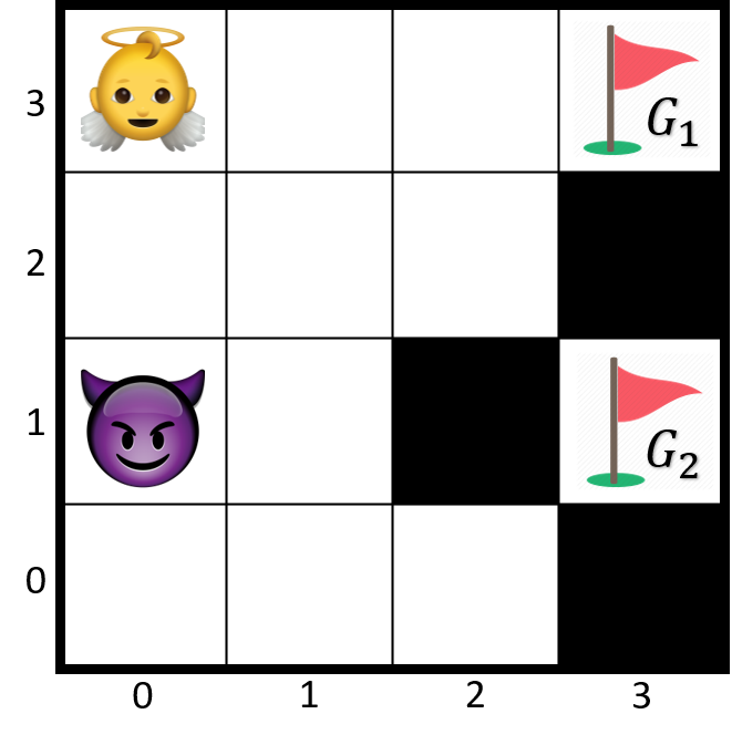
Figure 4: A game between a robot and its adversary on the gridworld.

A game on graph representing above scenario can be constructed using the product operation given in (Baier and Katoen, 2008, Def. 4.16). Every game state is a tuple $(x_{1},y_{1},x_{2},y_{2},t,q)$ where $x_{i},y_{i}$ for $i=1,2$ denote the cell that P1 and P2 occupy, $t$ represents the player who chooses the next move and $q$ denotes a state of a dfa that keeps track of the progress P1 has made towards completion of her objective. The resulting game has $4^{4}\times 2\times 4=2048$ states. We mark the states where P1 or P2 collide with an obstacle or with each other as the losing states for both players and, therefore, any action that leads to such states is disabled. Given the game on graph, a hypergame graph is constructed according to Def. 4. The hypergame graph has $2048\times 2=4096$ states because the adversary has two information states; $X_{0}$ and $X_{1}$.

When the above hypergame graph is given as an input to the Alg. 2, $2106$ out of $4096$ states are identified as dasw states. The projection of dasw states onto game state space results in $1172$ states, while the asw region has the size of $934$ states. This means that $1172-934=238$ game states that were almost-sure losing for P1 became winning for her, when P1 incorporated P2’s misperception into her planning to synthesize a deceptive strategy.

6 Conclusion

In this paper, we introduce a hypergame model to represent the interactions between two players with asymmetric information about their action capabilities. Then, we present an algorithm to synthesize action-deceptive strategies in a two-player turn-based zero-sum reachability games, where P2 has incomplete information about the P1’s action capabilities. We show that the synthesized strategy has two important and desirable properties. First, the dasw strategy is guaranteed to satisfy the reachability objective with probability one. Second, it is at least as powerful as the asw strategy, because the dasw region is a superset of the asw region.

References

- Baier and Katoen [2008] Christel Baier and Joost-Pieter Katoen. Principles of model checking. MIT press, 2008.
- Bennett [1977] PG Bennett. Toward a theory of hypergames. Omega, 5(6):749–751, jan 1977.
- Bernet et al. [2002] Julien Bernet, David Janin, and Igor Walukiewicz. Permissive strategies: from parity games to safety games. RAIRO - Theoretical Informatics and Applications, 36(3):261–275, 2002.
- Bloem et al. [2012] Roderick Bloem, Barbara Jobstmann, Nir Piterman, Amir Pnueli, and Yaniv Sa’ar. Synthesis of reactive(1) designs. Journal of Computer and System Sciences, 78(3):911 – 938, 2012. In Commemoration of Amir Pnueli.
- de Alfaro et al. [2007] Luca de Alfaro, Thomas A Henzinger, and Orna Kupferman. Concurrent reachability games. Theoretical Computer Science, 386(3):188–217, 2007.
- Ettinger and Jehiel [2010] David Ettinger and Philippe Jehiel. A theory of deception. American Economic Journal: Microeconomics, 2(1):1–20, February 2010.
- Fainekos et al. [2009] Georgios E. Fainekos, Antoine Girard, Hadas Kress-Gazit, and George J. Pappas. Temporal logic motion planning for dynamic robots. Automatica, 45(2):343 – 352, 2009.
- Gharesifard and Cortés [2012] Bahman Gharesifard and Jorge Cortés. Evolution of players’ misperceptions in hypergames under perfect observations. IEEE Trans. Automat. Contr., 57(7):1627–1640, 2012.
- Gharesifard and Cortés [2014] Bahman Gharesifard and Jorge Cortés. Stealthy deception in hypergames under informational asymmetry. IEEE Trans. Syst. Man, Cybern. Syst., 44(6):785–795, 2014.
- Gutierrez et al. [2015] Christopher N Gutierrez, Saurabh Bagchi, H Mohammed, and Jeff Avery. Modeling Deception In Information Security As A Hypergame–A Primer. In Proc. 16th Annu. Inf. Secur. Symp., page 41. CERIAS-Purdue University, 2015.
- Kovach [2016] Nicholas S Kovach. A Temporal Framework for Hypergame Analysis of Cyber Physical Systems in Contested Environments. Technical report, Air Force Institute of Technology, 2016.
- Kulkarni and Fu [2019] Abhishek Ninad Kulkarni and Jie Fu. Opportunistic synthesis in reactive games under information asymmetry. CoRR, abs/1906.05847, 2019.
- Pnueli and Rosner [1989] A Pnueli and R Rosner. On the synthesis of a reactive module. pages 179–190, 1989.
- Ramadge and Wonham [1989] P. J. G. Ramadge and W. M. Wonham. The control of discrete event systems. Proceedings of the IEEE, 77(1):81–98, Jan 1989.
- Rasmusen [1989] Eric Rasmusen. Games and information: An introduction to game theory. Number 519.3/R22g. Blackwell Oxford, 1989.