Lake Ice Detection from Sentinel-1 SAR with Deep Learning

Abstract

Lake ice, as part of the Essential Climate Variable (ECV) lakes, is an important indicator to monitor climate change and global warming. The spatio-temporal extent of lake ice cover, along with the timings of key phenological events such as freeze-up and break-up, provide important cues about the local and global climate. We present a lake ice monitoring system based on the automatic analysis of Sentinel-1 Synthetic Aperture Radar (SAR) data with a deep neural network. In previous studies that used optical satellite imagery for lake ice monitoring, frequent cloud cover was a main limiting factor, which we overcome thanks to the ability of microwave sensors to penetrate clouds and observe the lakes regardless of the weather and illumination conditions. We cast ice detection as a two class (frozen, non-frozen) semantic segmentation problem and solve it using a state-of-the-art deep convolutional network (CNN). We report results on two winters ($2016$-$17$ and $2017$-$18$) and three alpine lakes in Switzerland. The proposed model reaches mean Intersection-over-Union (mIoU) scores >90% on average, and >84% even for the most difficult lake. Additionally, we perform cross-validation tests and show that our algorithm generalises well across unseen lakes and winters.

1 INTRODUCTION

Climate change is one of the main challenges humanity is facing today, calling for new methods to quantify and monitor the rapid change in global and local climatic conditions. Various lake observables are related to those conditions and provide an opportunity for long-term monitoring, among them the duration and extent of lake ice. Remote sensing of lake ice also fits well with the Climate Change Initiative (CCI+, 2017) by the European Space Agency (ESA), where lakes and lake ice were newly included. Additionally, CCI+ promotes long-term trend studies and climate studies, as recognised by the Global Climate Observing System (GCOS). Furthermore, lake ice influences various economic and social activities, such as winter sports and tourism, hydroelectric power, fishing, transportation, and public safety (e.g., winter and spring flooding due to ice jams). In addition, its impact on the regional environment and ecological systems is significant, which further underlines the need for detailed monitoring.

Satellites are a secure source for remote sensing of the cryosphere and for sustainable, reliable, and long term trend analysis. Additionally, satellite images are currently the only means to monitor large regions systematically and with short update cycles. This increasing importance of satellite observations has also been recognised by the GCOS. Recently, Tom et al., (2018) proposed a machine learning-based semantic segmentation approach for lake ice detection using low spatial-resolution ($250$m-$1000$m) optical satellite data (MODIS and VIIRS). Although the nominal temporal resolution of those sensors is very good (daily coverage), the main drawback of this methodology is frequent data loss due to clouds, which reduces the effective temporal resolution. This is critical, since important phenological variables depend on frequent and reliable observation. In particular, the ice-on date is defined as the first day when the lake surface is (almost) completely frozen and remains frozen on the next day, and ice-off is defined symmetrically as the first day where a significant amount of the surface is liquid water, and remains in that state for another day (Hendricks Franssen, Scherrer, and Scherrer, 2008). The GCOS accuracy requirement for these two dates is $\pm 2$ days. Systems based on optical satellite data will fail to determine these key events if they coincide with a cloudy period. Moreover, low spatial resolution of MODIS and VIIRS is also a bottleneck for spatially explicit ice mapping. Higher resolution optical sensors like Landsat-8 or Sentinel-2 do not provide a solution, due to their low temporal resolution and susceptibility to clouds. On the contrary, Sentinel-1 represents a favourable trade-off between spatial and temporal resolution. Additionally, Radar is unaffected by clouds, which in many regions is a considerable advantage.

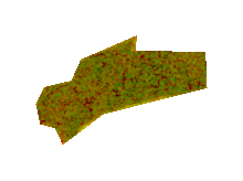
(a) Non-frozen (01.09.2016)

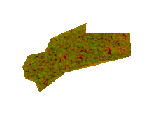
(b) Freeze-up (10.01.2017)

(c) Snow with skate tracks (08.02.2017)

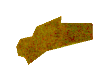
(d) Break-up (23.03.2017)

Figure 1: Examples of RGB composites of Sentinel-1 SAR data (RGB = [VV, VH, 0]) of lake St. Moritz showing the lake in the four different states specified in the sub-captions.

Here we propose to use Sentinel-1 SAR data, which mostly meets the requirements of lake ice monitoring, and additionally comes for free and with a commitment to ensure continuity of the observations. Its spatial and temporal resolution (GSD ca. 10 m / revisit period if 1.5 days) make it possible to derive high-resolution ice maps almost on a daily basis. For completeness, we mention that, taking into account estimation uncertainty, the temporal resolution of Sentinel-1 falls just short of the 1-day temporal resolution requirement of lake ice monitoring, it can still provide an excellent “observation backbone” for an operational system that could fill the gaps with optical satellite data (Tom et al.,, 2018) or webcams (Xiao et al.,, 2018).

Converting a Sentinel-1 image to a lake ice map boils down to 2-class semantic segmentation, i.e., assigning each lake pixel to one of two classes, frozen or non-frozen. We do this with the Deeplab v3+ semantic segmentation network (Chen et al.,, 2018). Examples of Sentinel-1 SAR composites over the lake St. Moritz is visualised in Fig. 1, showing the VV amplitude in the red channel, and the VH amplitude in the green channel. The examples include the states non-frozen (01.09.2016, water), freeze-up (10.01.2017), frozen (08.02.2017, snow on top of ice) and a break-up date (23.03.2017).

Target lakes and winters. We analyse three selected lakes in Switzerland (Sils, Silvaplana, St. Moritz, see Table 1) over the period of two winters ($2016$-$17$ and $2017$-$18$). These three lakes are located close to each other in the same geographic region, referred to as Region Sils. The lakes are comparatively small and situated in an Alpine environment, and they are known to reliably freeze over completely every year during the winter months. For the two winters $2016$-$17$ and $2017$-$18$, all available images were collected for the nine months between September $1$ and May $31$. After back-projecting the digitised lake outline polygons from Open Street Map (OSM) on to the SAR images, for each lake, we extract the lake pixels which lie inside the lake outline. In low-spatial resolution satellite images such as MODIS and VIIRS, only few such lake pixels are available (Tom et al.,, 2018), which makes the analysis of very small lakes such as St. Moritz difficult or even impossible. Thanks to the higher spatial resolution, the Sentinel-1 time series provides us with millions of lake pixels, which makes it possible to train powerful deep learning models for segmentation, which are extremely data-hungry.

Contributions. We address the problem of lake ice detection from Sentinel-1 SAR data, as an alternative to optical satellite data which is impaired by clouds. In the process, we show that a deep learning model pre-trained on an optical RGB dataset can nevertheless be re-used successfully as initialisation for fine-tuning to Radar data. To our knowledge, our work is the first one that utilises Radar data and deep learning for lake ice detection, though it has been used for sea ice analysis.

	Sils	Silvaplana	St. Moritz
Area ($km^{2}$)	$4.1$	$2.7$	$0.78$
Altitude (L) ($m$)	$1797$	$1791$	$1768$
Max. depth ($m$)	$71$	$77$	$42$
Meteo station	Segl Maria	Segl Maria	Samedan
Dist. to lake ($km$)	0.5	1	5
Altitude (S) ($m$)	$1804$	$1804$	$1709$

Table 1: Characteristics of the target lakes. Altitude (L) and altitude (S) denote the altitudes of the lake and nearest meteo station respectively. The distance to station is also shown.

Lake	Winter	Non-transition days		Transition days	Total	Temporal resolution (days)	# lake pixels
		Non-frozen	Frozen		# acq.
Sils	2016-17	40	42	37	119	2.3	40908
	2017-18	76	65	40	181	1.5
Silvaplana	2016-17	36	44	39	119	2.3	26563
	2017-18	85	66	30	181	1.5
St. Moritz	2016-17	66	42	11	119	2.3	7521
	2017-18	84	77	20	181	1.5

Table 2: Dataset statistics. Non-transition days, on which a lake is almost fully frozen / non-frozen, and transition days (partially frozen) are shown. Lake pixels are those which lie completely inside the lake polygon. # acq. denotes the number of acquisitions.

2 RELATED WORK

Many studies discussed the trends in lake ice formation in different parts of the globe. Duguay et al., (2006) presented the trends in lake freeze-up and break-up across Canada for a long period from $1951$ until $2000$. Later, Hendricks Franssen, Scherrer, and Scherrer (2008) reported the decreasing tendency in lake freezing in several Swiss lakes. Then, Brown, Duguay, and Duguay (2010) reviewed the response and role of ice cover in lake-climate interactions. This paper observed that the ability to accurately monitor lake ice will be an important step in the improvement of global circulation models, regional and global climate models and numerical weather forecasting. Brown, Duguay, and Duguay (2011) used the Canadian Lake Ice Model (CLIMo) to simulate lake ice phenology across the North American Arctic from $1961$–$2100$, using two climate scenarios produced by the Canadian Regional Climate Model (CRCM). They projected changes to the ice cover using $30$-year mean data between $1961$–$1990$ and $2041$–$2070$, which suggested a probable drift in freeze-up ($0$–$15$ days later) and break-up ($10$–$25$ days earlier). Duguay et al., (2015) presented an overview of the progress of remote sensing for lake and river ice. For lakes, that work reviewed a number of topics, including ice cover concentration, ice extent and phenology, and ice types, as well as ice thickness, snow on ice, snow/ice surface temperature, and grounded and floating ice cover on shallow Arctic and sub-Arctic lakes.

Lake ice monitoring using Radar data. Duguay, Lafleur, and Lafleur (2003) proposed to determine the depth and thickness of ice in shallow lakes and ponds using the Landsat Thematic Mapper and European Remote Sensing (ERS)-1 SAR data. Almost a decade later, Surdu et al., (2014) conducted a study of the shallow lakes on the north slope of Alaska to find the response of ice cover on the climate conditions using Radar remote sensing and numerical analysis. A machine learning-based automated ice-vs-water classification was proposed by Leigh et al., (2014) using dual polarisation SAR imagery. Later, Surdu et al., (2015) performed a study on the ice freezing and thawing detection in shallow lakes from Northern Alaska with spaceborne SAR imagery. Antonova et al., (2016) monitored ice phenology in lakes of the Lena river delta using TerraSAR-X backscatter. Du et al., (2017) performed an assessment of lake ice phenology in the Northern Hemisphere from $2002$ to $2015$. Pointner et al., (2018) studied the effect of the lake size on the accuracy of a threshold-based classification of ground-fast and floating lake ice from Sentinel-1 SAR data. Duguay, Wang, and Wang (2019) presented various algorithms such as thresholding, Iterative Region Growing with Semantics (IRGS) and $k$-means for the generation of a floating lake ice product from Sentinel-1 SAR data for various permafrost regions (Alaska, Canada and Russia). Geldsetzer et al., (2010) used RADARSAT-2 SAR data to monitor ice cover in lakes during the spring melt period in the Yukon area of the Canadian Arctic. They put forward a threshold-based classification methodology and observed that the HH and HV backscatter from the lake ice have significant temporal variability and inter-lake diversity. Murfitt et al., (2018) used the RADARSAT-2 imagery to develop a threshold-based method to determine lake phenology events for the mid-latitude lakes in Central Ontario from $2008$ to $2017$. Wang et al., (2018) also used RADARSAT-2 imagery (dual polarised) for developing a lake ice classification system acquired over lake Erie, with the IRGS method. Additionally, Gunn et al., (2018) used the polarimetric RADARSAT-2 (C-Band) to observe the scattering mechanisms of bubbled freshwater lake ice. SAR data analysis is challenging, and deep learning could play a significant role because of its ability to learn task-specific, hierarchical image features.

Lake ice monitoring with webcams. Xiao et al., (2018) described a system that detects lake ice in webcam data with the help of a deep neural network. Public webcams have two main advantages compared to optical satellite images. Firstly, they are usually not affected by clouds, except for the comparatively rare case of dense fog. Secondly, they have a very high temporal resolution (up to one image per 10 min). Although the approach generated excellent results, it also has disadvantages. Webcams are usually placed arbitrarily (e.g., too far away or covering a small lake area), and often only low above the lake, leading to great scale differences between front and back of the lake surface. Moreover, they are prone to hardware failure, and, being very cheap cameras, they have poor spectral and radiometric quality with significant compression artifacts. Another practical problem with webcams is that it is difficult to operationalise them at country- or even world-scale.

Optical data for lake ice monitoring. Tom et al., (2018) proposed a machine learning-based methodology for lake ice detection using low resolution optical satellite images. The main problem with optical satellite images is the data loss due to clouds. However, the authors showed that the algorithm produces consistent results when tested on data from multiple winters. In addition, Barbieux et al., (2018) used Landsat-8 multi-spectral data for extraction of frozen lakes and water-vs-ice classification. Recently, Tom et al., (2019) put forward a feasibility study, which targeted for a unified lake ice monitoring system that combines images from optical satellites, in-situ temperature data and webcam images.

3 data

Sentinel-1 SAR consists of two identical satellites (S1A and S1B) operational in space with $180^{\circ}$ phase shift, following a sun-synchronous, near-polar orbit. The two satellites orbit the Earth at an altitude of $693$ km and have a repeat cycle of $12$ days at the equator (effectively $6$ days with S1A and S1B). The same point on Earth is mapped several times within one repeat cycle. Due to the large across-track area coverage of the satellites and the latitude of our target area in Switzerland (and most other areas where lakes freeze), the revisit time is further reduced. For Region Sils, it can bee seen from Table 2 that the temporal resolution in winter $2017$-$18$ is better than that of $2016$-$17$. This is because of missing data from S1B. Though S1B was launched in April 2016, the corresponding data is fully available in the Google Earth Engine (GEE) platform (see Section “Data Collection” below) only from March $2017$. In addition, Sentinel-1 covers the Region Sils in four orbits. See Table 3 for the details. Footprints of the four orbits are shown in Fig. 2.

Table 3: Details of four orbits scanning Region Sils such as orbit number, flight direction, acquisition time in Universal Coordinate Time (UTC), and approximate incidence angle.

Orbit	Flight dir.	Acquisition time	Incidence angle
15	ascending	17:15	41.0∘
66	descending	05:35	32.3∘
117	ascending	17:06	30.8∘
168	descending	05:26	41.7∘

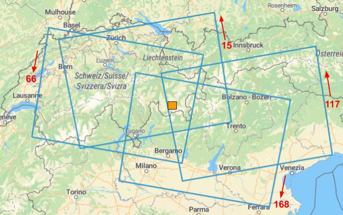
Figure 2: The four Sentinel-1 orbits ($15$, $66$, $17$, $168$) with the corresponding directions (ascending or descending) which covers the Region Sils (shown as orange filled rectangle).

The S1A and S1B satellites have the same SAR system on board which sends out frequency-modulated electromagnetic waves (C-frequency band) and detects the backscattered echoes of the surface. From the reflected signal, the SAR sensor measures the amplitude and phase. In our research, we use only the amplitude information. We work with the Level-1 Ground Range Detected (GRD) product in Interferometric Wide (IW) swath mode. That product has no phase information anymore, and has a nearly square footprint ($10$m$\times 10$m per pixel). It also has good temporal resolution (see Table 2) and four polarisations (VV, VH, HH, HV). However, for the Region Sils, data is acquired only in VV and VH modes. The distribution of backscatter values of frozen and non-frozen pixels in these bands are shown in Fig. 3. Note that the separability in VV appears better than in VH.

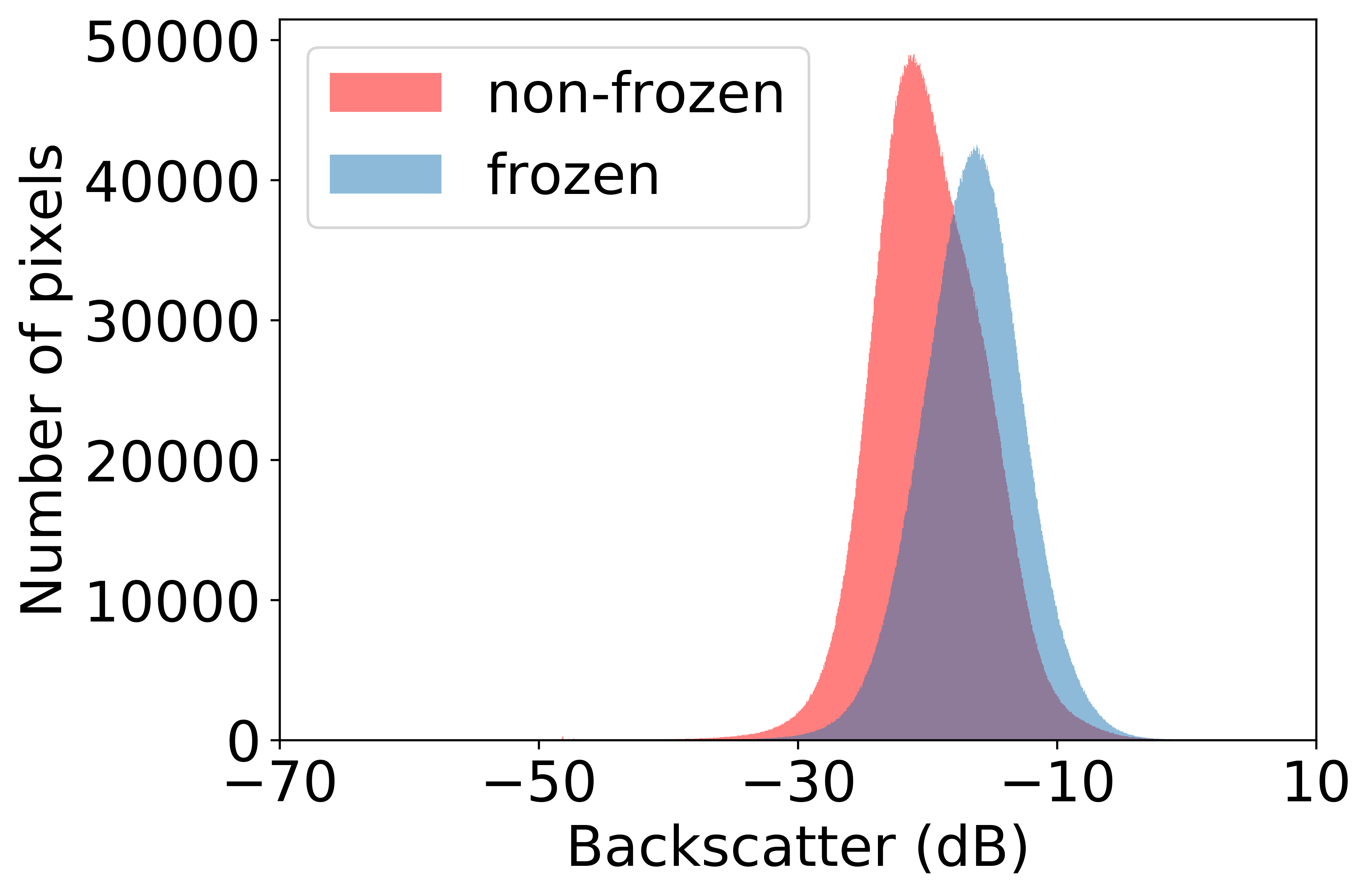
(a) Distribution of VV

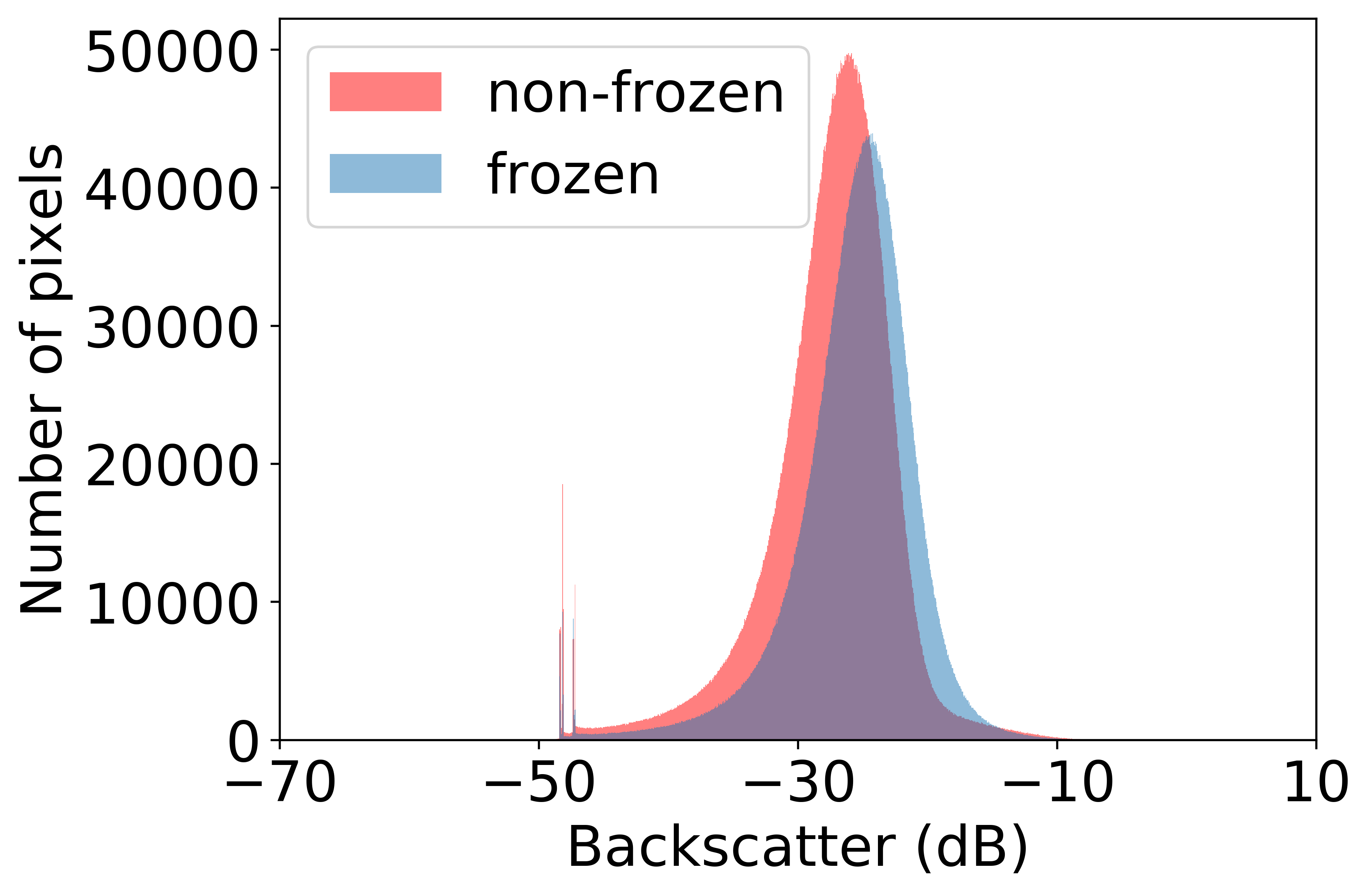
(b) Distribution of VH

Figure 3: Distribution of frozen and non-frozen pixels for VV and VH polarisations (combined data from $3$ lakes, $2$ winters). Best if viewed on screen.

The radar backscatter is influenced in a complex manner by a variety of factors, which can be grouped into two main categories. Firstly, the sensor parameters such as wavelength ($5.54$ cm), incident angle ($20^{\circ}$ to $46^{\circ}$) and polarisation. Secondly, it depends on surface parameters which can be either geometrical factors such as roughness, landscape topography, etc. or physical factors such as the permittivity of the surface material. Significant factors for lakes are also wind speed and direction, and the water content in snow. For smooth and plain water, almost all radiation is scattered away from the sensor making it appear very dark. As the wind speed picks up, waves occur on the water surface and significant scattering can occur. When perfectly plain water is covered by perfectly plain ice, microwaves penetrate the ice without absorption and are reflected at the ice-water interface away from the sensor, and the ice covered lake would in theory appear completely black. In reality, cracks in the ice scatter some microwaves back to the sensor. Therefore, visible and well located cracks are clear indicators for ice cover. Furthermore, in reality, the ice-water interface is never completely smooth, therefore some scattering can occur at these boundaries which, however, can be weak. The older the ice, the more air bubbles are enclosed in it, which increase the backscatter within the ice volume by direct backscattering and also by double reflection of microwaves at the air-bubbles and the ice-water interface. With snow cover, the air-ice interface becomes increasingly rough which further increases the backscatter signal. Finally, with snow melt, the liquid water content of the overlying snow pack increases and significantly reduces the backscatter signal, as the snow-water mixture of wet snow absorbs a significant fraction of the microwave energy.

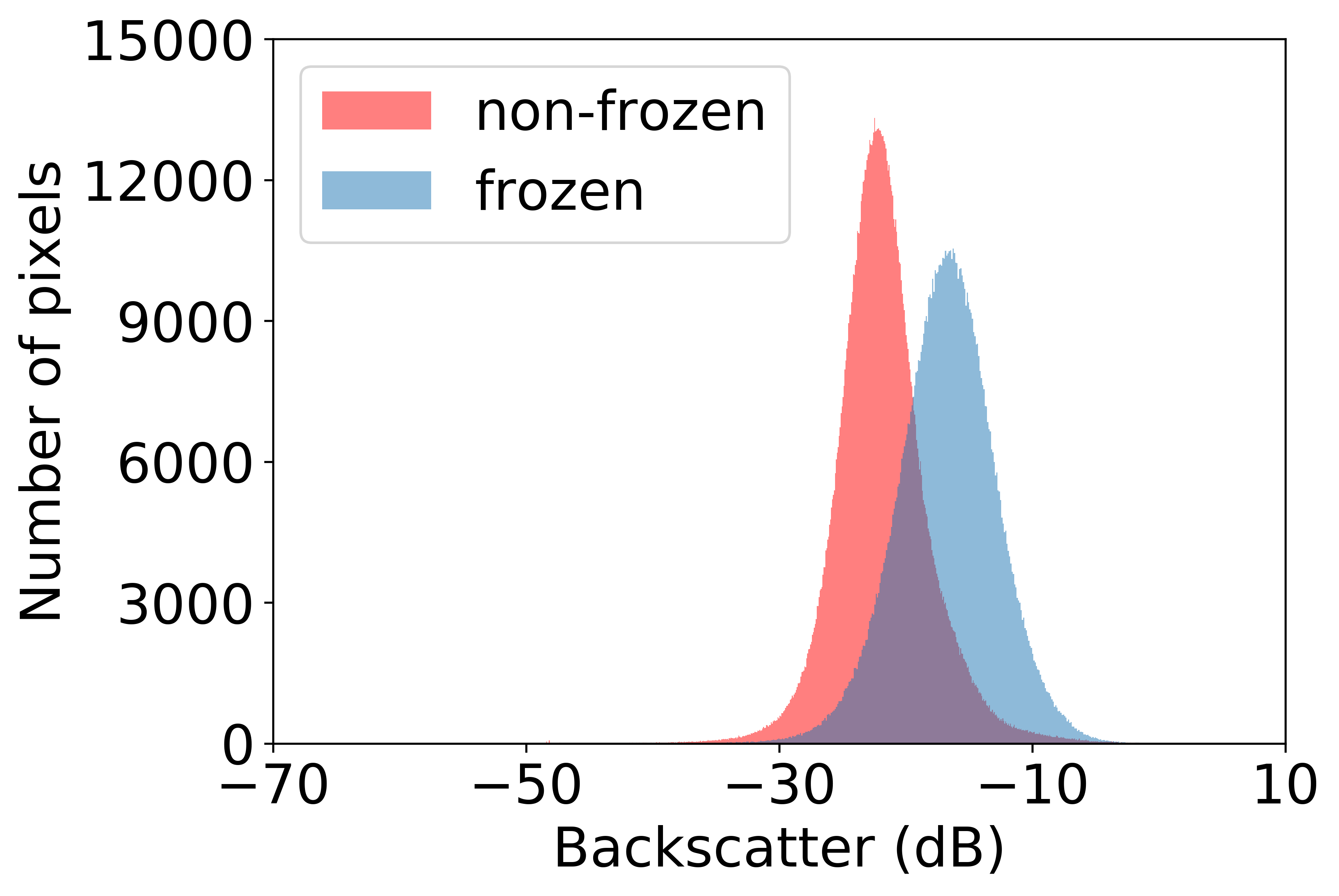
(a) VV, wind speed <5 Km/h

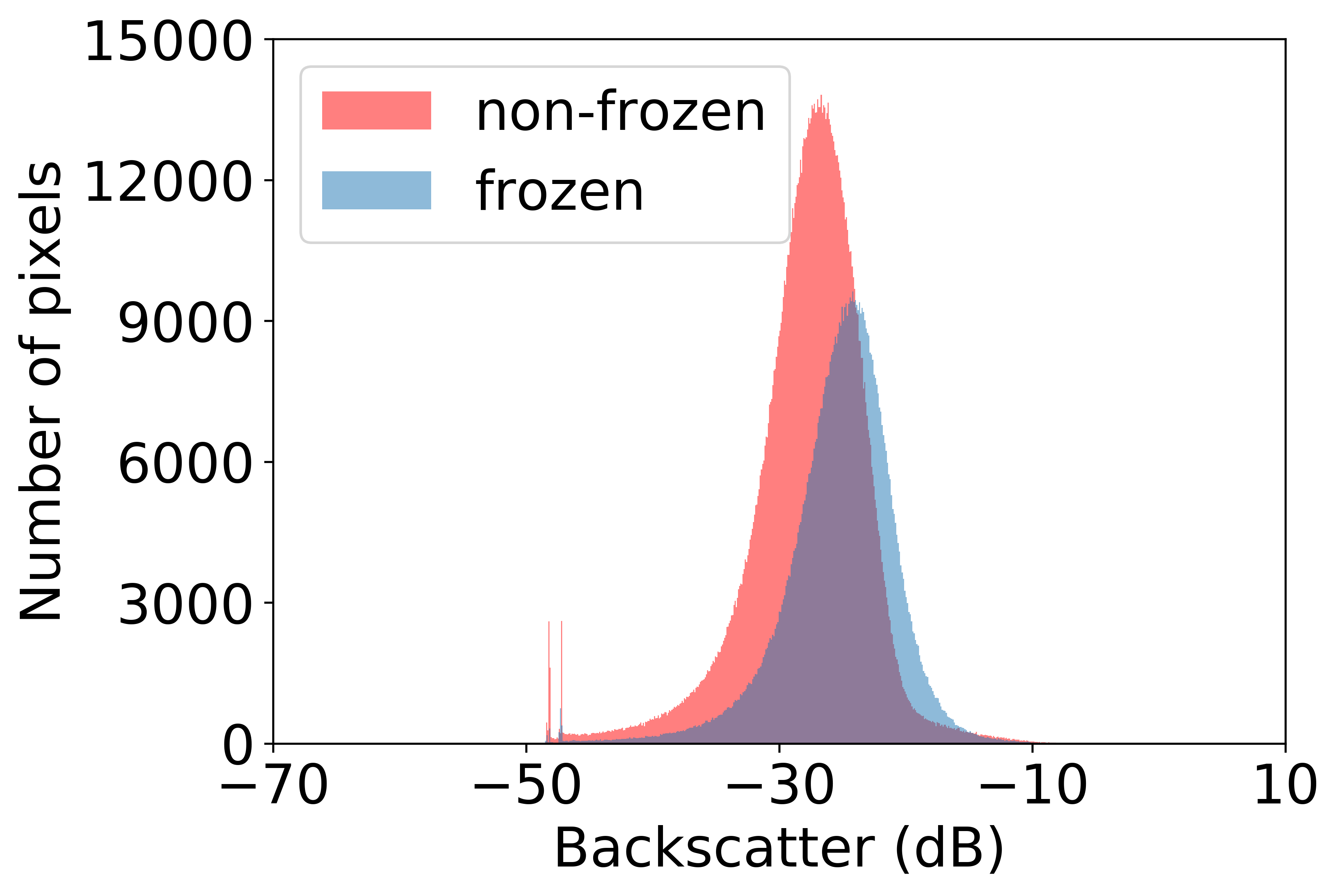
(b) VH, wind speed <5 Km/h

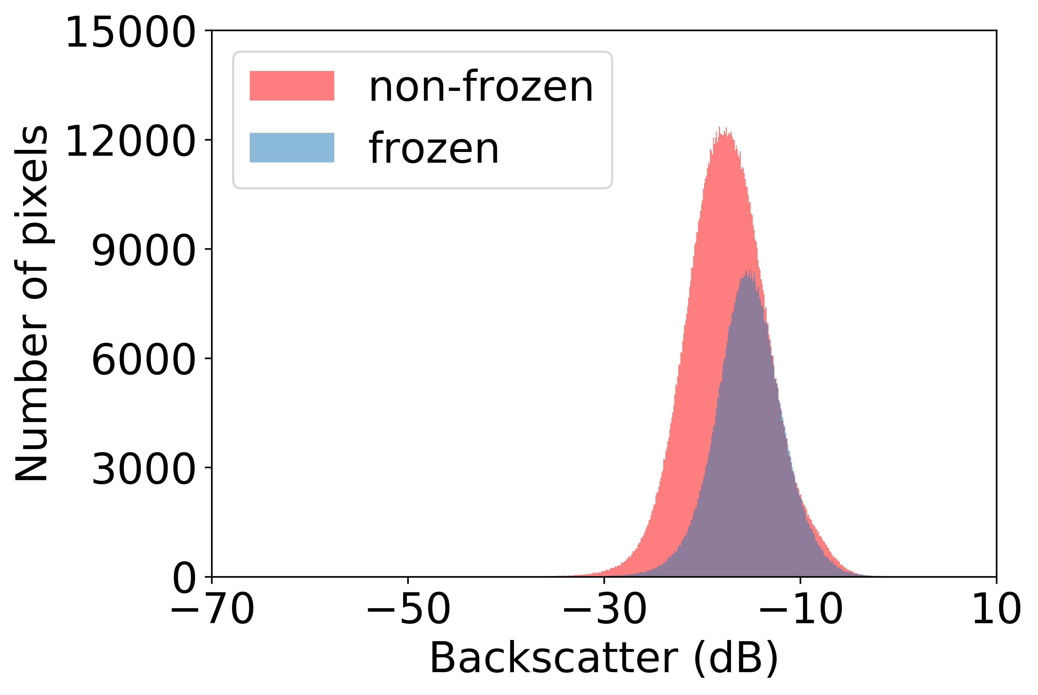
(c) VV, wind speed >20 Km/h

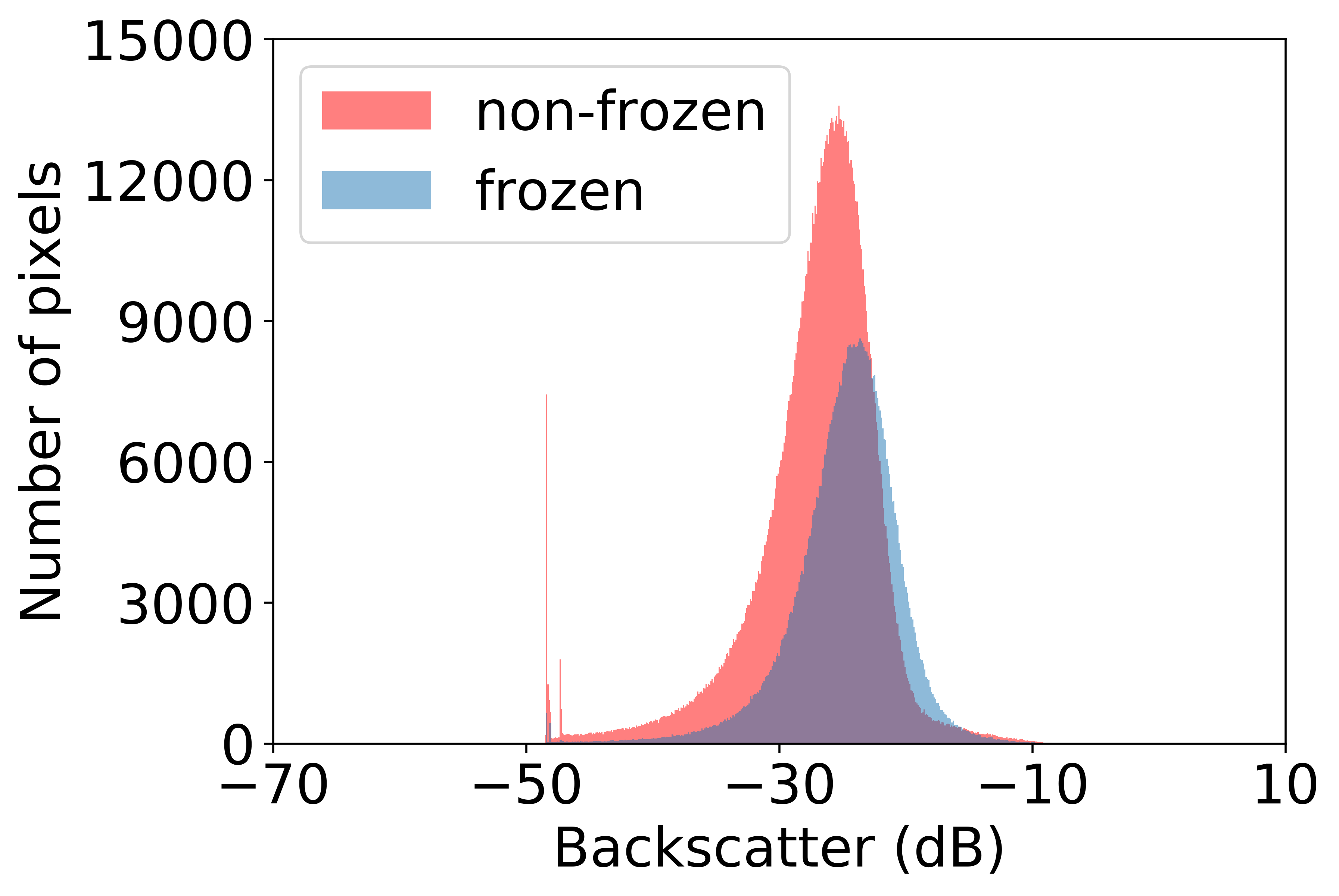
(d) VH, wind speed >20 Km/h

Figure 4: Distribution of frozen and non-frozen pixels for VV and VH polarisations in different wind speed conditions (combined data from $3$ lakes, $2$ winters). Best if viewed on screen.

Data collection and pre-processing. GEE is a cloud-based platform for large-scale geo-spatial data analysis (Gorelick et al.,, 2017). It stores and provides data of various satellite missions, performs data pre-processing and makes them freely available for education and research purposes. The Sentinel-1 backscatter coefficients (in decibels) were downloaded from the GEE platform after several inbuilt pre-processing steps such as GRD border noise removal which corrects the noise at the border of the images, thermal noise removal for correcting the thermal noise between the sub-swaths, radiometric calibration which calculates the backscatter intensity using the GRD metadata, terrain correction to correct the side looking effects using the digital elevation model (SRTM, 30m), and log-scaling to transform the approximate distribution of the SAR responses from Chi-squared to Gaussian (see Fig. 3). Note that we did not perform any absolute geolocation correction, since the back-projected lake outlines suggested a sufficient accuracy.

Transition and non-transition days. All the data from two winters was divided into two categories: non-transition dates where the lake is almost fully frozen or fully non-frozen, and transition dates with partially frozen lake surface. Both freeze-up and break-up dates belong to the transition category. The dataset statistics are shown in Table 2. Note that, since lake St. Moritz is relatively small in area and volume, it freezes and melts faster and has fewer transition days.

Ground truth. For each lake, one label (fully frozen / non-frozen, partially frozen / non-frozen) per day was assigned by a human operator after visual interpretation of the visible part of the lake from freely available webcam data. The ground truth thus generated was further enriched by visual interpretation of the Sentinel-2 images whenever available. However, some remaining noise in the ground truth is likely due to interpretation errors, as a result of overly oblique viewing angles of webcams and compression artefacts in the images. During the transition days, ground truth estimation was very difficult since we had partially frozen and non-frozen states and there was a difficulty to discriminate transparent ice and water. Thus, transition days were not used for quantitative analysis.

4 Methodology

Semantic segmentation. We define lake ice detection as a two class (frozen, non-frozen) pixel-wise classification problem and tackle it with the state-of-the-art semantic segmentation network Deeplab v3+ (Chen et al.,, 2018). The non-frozen class comprises of only water pixels. Whereas a pixel is considered to be part of the frozen class if it is either ice or snow, since in the target region, the frozen lakes are covered by snow for much of the winter. The standard procedures in machine learning-based data analysis are followed. The dataset is first divided into mutually exclusive training and test sets. The Deeplab v3+ model is then fitted on the training set. Lastly, the trained model is tested on the previously unseen test dataset.

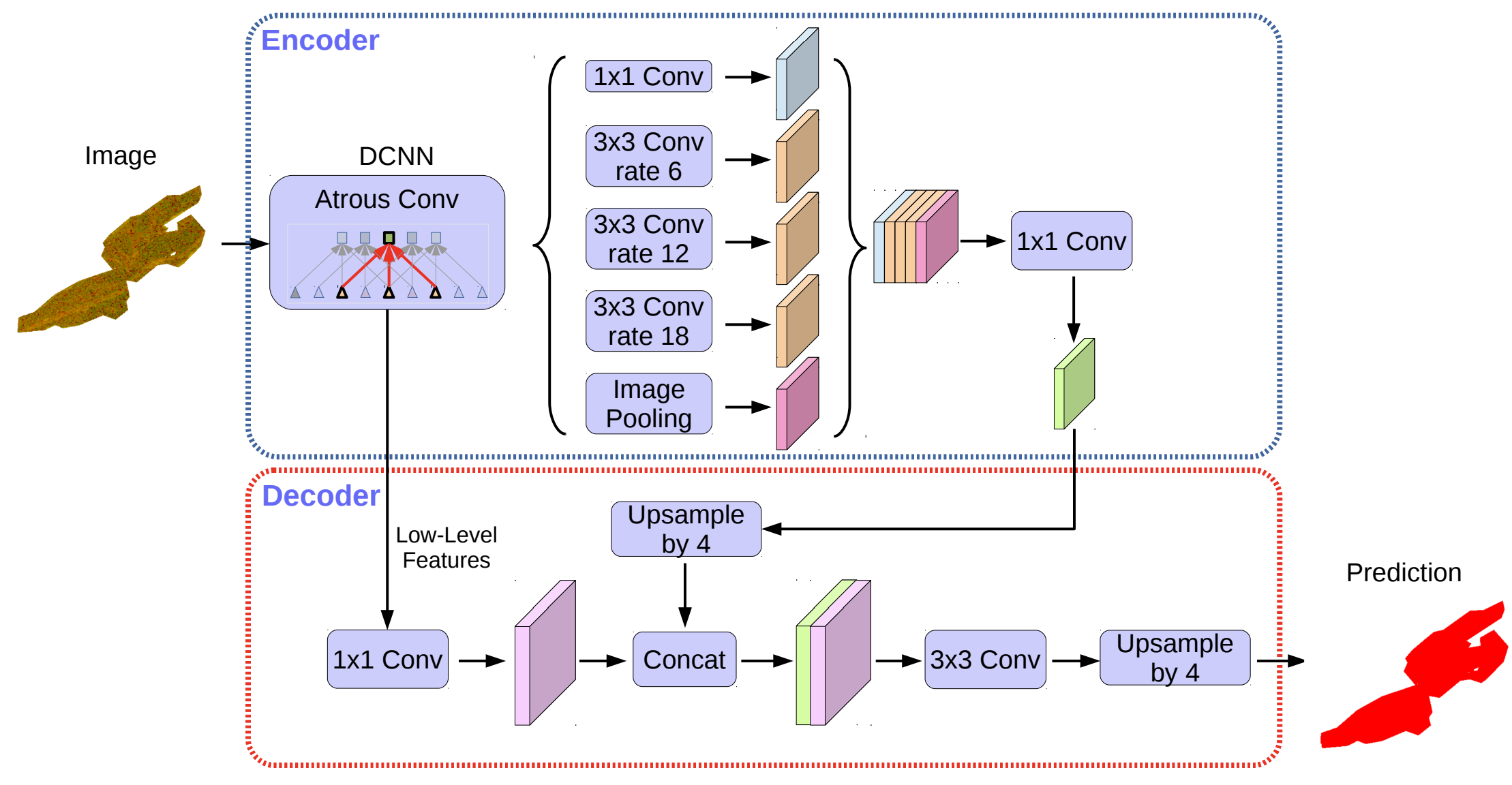
Figure 5: Deeplab v3+ architecture. Best if viewed on screen.

	Non-frozen   Frozen	Recall
Non-frozen	3.06         0.01	99.7%
Frozen	0.29         2.89	90.8%
Precision	91.3%      99.6%	95.5%

	Non-frozen   Frozen	Recall
Non-frozen	5.77         0.19	96.7%
Frozen	0.44         4.59	91.1%
Precision	92.9%      95.8%	94.8%

Table 4: Results for winter $2016$-$17$ (left) and $2017$-$18$ (right). Data from all the three lakes from winter $2016$-$17$ was used to train the model that was tested on winter $2017$-$18$, and vice versa. Confusion matrices are shown. Units are in millions of pixels, except for precision, recall, and accuracy (bottom right cell in each table).

Deeplab v3+ (Chen et al.,, 2018) is a deep neural network for semantic segmentation, which has set the state-of-the-art in multiple benchmarks, including among others the PASCAL VOC 2012 dataset (Everingham et al.,, 2015). It combines the advantages of both Atrous Spatial Pyramid Pooling (ASPP) and encoder-decoder structure. Atrous convolution allows to explicitly control the resolution of the features computed by the convolutional feature extractor. Moreover, it adjusts the field-of-view of the filters in order to capture multi-scale information. Deeplab v3+ also incorporates depthwise separable convolution (per-channel 2D convolution followed by pointwise $1\times 1$ convolution) which significantly reduces the model size. The network architecture is shown in Fig. 5.

Network parameters. We used the mobilenetv2 implementation of Deeplab v3+, as available in TensorFlow. The train crop size was set to $129\times 129$ (effective patch size is $128\times 128$) and the eval crop size to the full image resolution. All models were trained for $40^{\prime}000$ iterations with a batch size of $8$. Atrous rates were set to [$1,2,3$] for all experiments. The cross-entropy loss function was minimised with standard stochastic gradient descent, with a base learning rate of $10^{-3}$.

Transfer learning. Deep supervised classification approaches need lots of labelled data and a large amount of resources to train a model from scratch. Such data volumes are often not available. Even if they are, labelling them is costly and increases the computational cost of model training. Transfer learning mitigates this bottleneck by using an already trained model from some related task as a starting point. Given the fact that the initial layers of a neural network learn rather generic local image properties, a model trained on a huge image dataset can be re-utilised on a different dataset with a much smaller amount of fine-tuning (re-training) to the specific characteristics of the new data. We use a Deeplab v3+ model pre-trained on the PASCAL VOC 2012 close-range dataset as the starting point and fine-tune it on the relatively small Sentinel-1 SAR dataset (see Table 2). Surprisingly, we find that pre-training on RGB amateur images of indoor scenes, vehicles, animals, humans etc. greatly enhances the performance even on a data source as different as interferometric Radar, compared to training from scratch only on the SAR data. Note, all weights were fine-tuned, we did not freeze any network layers.

5 EXPERIMENTS, RESULTS, AND DISCUSSION

We use various measures to quantify performance, including recall, precision, overall accuracy, and the IoU score (Jaccard index). In all experiments described in the paper, we used only lake pixels from the non-transition dates to train the network and to compute performance metrics. This is due to the lack of reliable ground truth during the transition dates. Additionally, whenever the ground truth cannot be established for a non-transition date due to foggy webcam images and/or clouds in Sentinel-2, it is exempted from the training set. However, qualitative analysis is done on all the dates.

Quantitative results: Semantic segmentation. For developing an ideal operational system for lake ice monitoring, the data from a couple of lakes from a few winters would have to be used to train the model, which can then be deployed on unseen lakes and winters. However, generating ground truth for each lake is a tedious task. Nevertheless, we make sure that the data from at least one lake from one full winter is in the training set for the classifier to learn the proper class decision boundaries.

We employ Cross-Validation (CV), i.e., the data is partitioned into k folds, usually of approximately the same size. Then, the evaluation is done k times, each time using one fold as test set and the union of all remaining folds as training set. Leave-one-out cross-validation is the setting where the number of folds equals the number of instances (in our case the number of winters/lakes) in the dataset.

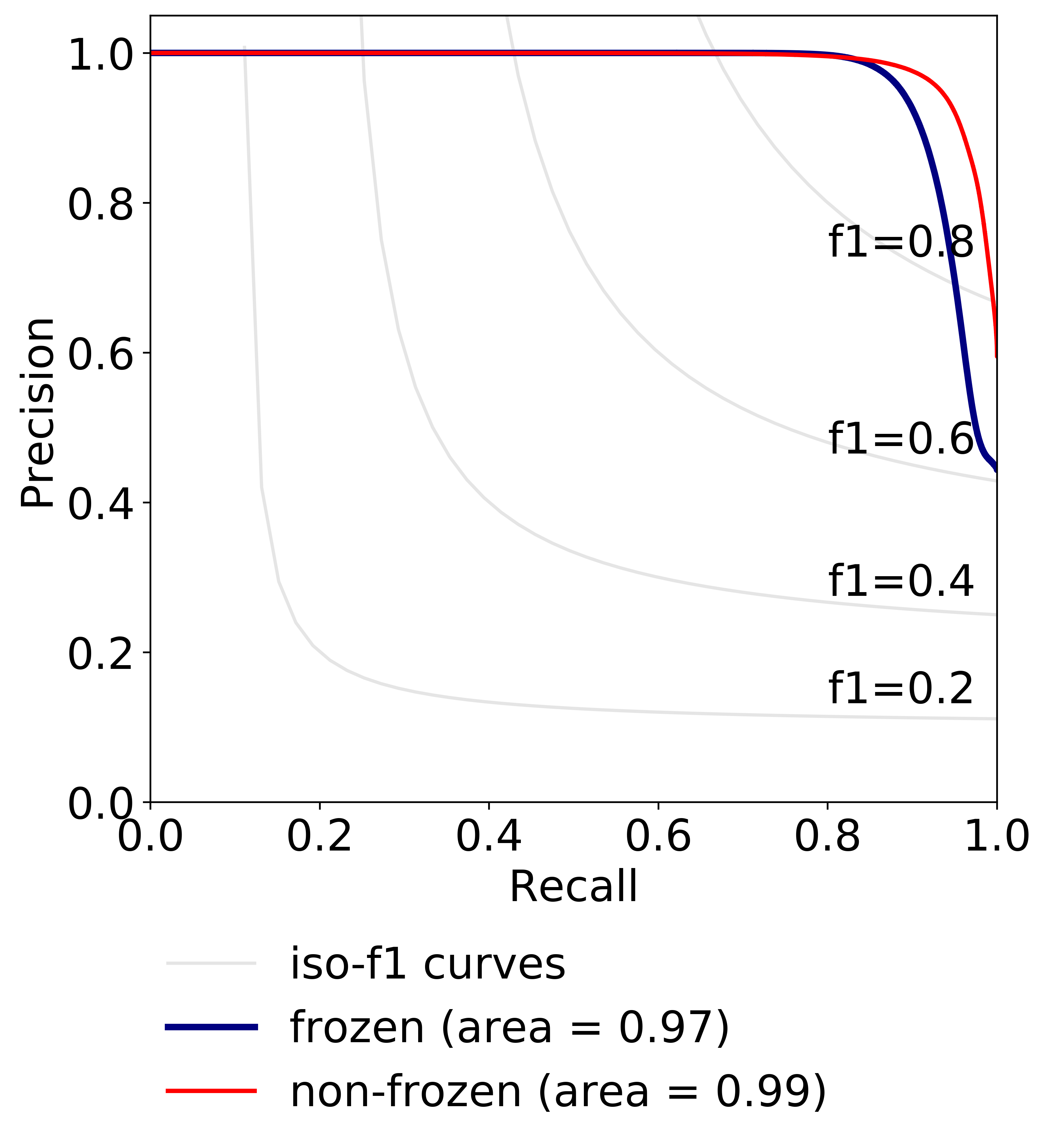
Figure 6: Precision-recall (PR) curves for lakes Sils (left), Silvaplana (middle), and St. Moritz (right) for winter $2017$-$18$. The iso-f$1$ curve connects all points in the PR space with same F$1$ score. Combined data of all $3$ lakes from winter $2016$-$17$ was used to train the model. Best if viewed on screen.

The goal of leave-one-winter-out CV is to investigate the generalisation capability of a model trained on one winter when tested on a different winter. The results are shown on Table 4. It can be seen that we achieve excellent results for both winters with average accuracies of $95.5\%$ and $94.8\%$ for $2016$-$17$ and $2017$-$18$ respectively. The results show that the model generalises well across the potential domain shift caused by the specific conditions of different winters, without having seen data from any day within the test period.

	Non-frozen   Frozen	Recall
Non-frozen	4.69         0.02	99.4%
Frozen	0.13         4.22	96.9%
Precision	97.3%      99.4%	98.3%

	Non-frozen   Frozen	Recall
Non-frozen	3.08         0.10	96.4%
Frozen	0.11         2.78	96.1%
Precision	96.4%      96.4%	96.4%

	Non-frozen   Frozen	Recall
Non-frozen	1.00         0.10	94.1%
Frozen	0.62         0.82	88.5%
Precision	94.1%      88.5%	91.5%

Table 5: Results for lake Sils (top), Silvaplana (middle), and St. Moritz (bottom). Confusion matrices are shown for the leave-one-lake-out cross-validation experiment. Units are in millions of pixels, except for precision, recall, and accuracy (bottom right cell in each table).

We also report results of a leave-one-lake-out CV experiment to check the generalisation capacity of the model across lakes. The results are shown on Table 5. While testing for all data of a lake (e.g., Sils) from two winters, the data from the other two lakes (e.g., Silvaplana, St. Moritz) from the same two winters is used for training. The prediction achieves >$91.5\%$ overall accuracy for all three lakes. See Table 6 for the per-class and mean IoU values for each lake. The worst performance is noted for St. Moritz where the lake itself is smaller than the size of a single patch ($128\times 128$). Note also, St. Moritz has the least mIoU, especially for class frozen. This is because of the presence of tents and other infrastructure on the frozen lake St. Moritz, which is not present in the other two lakes used in training. To assess the per-class performance in detail, we also report the precision-recall curves in Fig. 6. For both the frozen and non-frozen classes, the area under the curve is nearly optimal for lake Sils and very good performance is achieved on lakes Silvaplana and St. Moritz.

Table 6: Per-class- and mean IoU values of frozen and non-frozen classes for each lake. The data of a lake from two winters ($2016-17$ and $2017-18$) is tested using a model trained on the data from the other two lakes from both winters.

	Sils	Silvaplana	St. Moritz
Non-frozen	96.7%	93.3%	85.6%
Frozen	96.4%	92.7%	82.9%
Mean	96.5%	93.1%	84.3%

Quantitative results: Time-series. The ice-on and ice-off dates are of particular interest for climate monitoring. From the per-day semantic segmentation results, we estimate the daily percentage of frozen surface for each observed lake. Thus, for each available SAR image, we compute the percentage of frozen pixels, throughout the entire winter. An example time series for lake Silvaplana in winter $2017$-$18$ is shown in Fig. 7a. Although we do not have per-pixel ground truth on the partially frozen transition days, we know whether the lake has more water (shown with a value of $75\%$ in the ground truth) or more ice/snow (shown with a value of $25\%$ in the ground truth). Even though some miss-classifications exist during the transition days, the non-transition days are almost always predicted correctly, likely because the network was trained solely on non-transition days. For a comparison, we also plot the time series of temperature values (sliding window mean of the daily median, window size $7$ days) obtained from the nearest meteo station in Fig. 7b. Sub-zero values in this graph correlate (with some time lag) with the period in which the lakes are fully or partially frozen.

(a) Time series of percentage of non-frozen pixels for lake Silvaplana from winter $2017$-$18$.

(b) Temperature (temporal moving average of daily median with window size of $7$ days) from the nearest meteo station.

Figure 7: Correlation of our results (winter $2017$-$18$) on lake Silvaplana with the ground truth and the auxiliary temperature data. Best if viewed on screen.

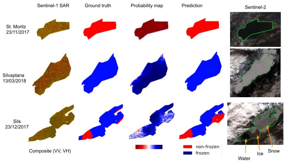
Figure 8: Qualitative results for lake St. Moritz on a non-frozen day (row $1$), lake Silvaplana on a frozen day (row $2$), and lake Sils on a transition day (row $3$). For each lake we show the Sentinel-1 composite image (column $1$), the ground truth (column $2$), the predicted frozen probability map derived from the network logits (column $3$), and the corresponding binary classification map (column $4$). Additionally, column $5$ shows a corresponding Sentinel-2 image for better visual interpretation.

Qualitative analysis. Exemplary qualitative results are depicted in Fig. 8. We show the classification results on frozen, non-frozen, and transition dates along with the probability map (blue means higher probability of frozen, red means higher probability of non-frozen). For better interpretation of the result, especially for the transition date, we show the corresponding image from Sentinel-2.

Table 7: Per-class- and mean IoU values of frozen and non-frozen classes with different polarisations (left table) and orbits (right table). Data from all three lakes from winter $2016$-$17$ was tested using a model trained on the data from all three lakes from winter $2017$-$18$. Asc and Dsc denotes ascending and descending orbits respectively.

	VV, VH	VH	VV	VV, VV_prev
Non-frozen	91.0%	71.0%	87.7%	93.3%
Frozen	90.6%	60.1%	86.6%	91.9%
Mean	90.8%	65.9%	87.1%	92.6%

	Asc, Dsc	Dsc	Asc
Non-frozen	91.0%	84.7%	85.9%
Frozen	90.6%	82.7%	84.3%
Mean	90.8%	83.7%	85.1%

Miscellaneous experiments. In all the experiments reported so far, we used the data from all four orbits (both ascending and descending) and both polarisations (VV and VH). To study the individual effect of polarisations VV and VH, we drop either of them and report the corresponding results on Table 7 (left). Note that mIoU drops by almost $25\%$ when VV is left out, while it drops by only $3.7\%$ without VH, confirming the significance of polarisation VV for lake ice detection. This finding also aligns with the visual differences in Fig. 3. However, while VH appears to be less discriminative overall, it is much less affected by wind speed – see Fig. 4. We believe that using also VH may improve robustness in windy conditions, where discriminating water from ice/snow should be particularly challenging because of increased surface roughness due to waves. However, we do not have enough days with strong wind to quantitatively corroborate this hypothesis. From our current data it appears that the system can handle calm and moderately windy days practically equally well.

In another experiment, we drop VH but use VV from two temporally adjacent acquisitions (VV and VV_prev), thus simultaneously feeding the network with data from two different days. The mIoU rises by  $2\%$, see Table 7 (left). However, we noted some stability issues especially during fully frozen days. We believe this is due to the fact we removed VH. We did another experiment to check the effect of acquisition time. Here, we used the data from both VV and VH. However, we drop the data from some orbits (see Table 3). Table 7 (right) shows that the mIoU drops by $7.1\%$ and $5.7\%$ respectively when the data from only descending orbits ($66$ and $168$) or only ascending orbits ($15$ and $117$) were used. A final experiment was done to assess the influence of the (rectangular) training patch size, see Fig. 9. Somewhat surprisingly, even the move from an already large context of $64\times 64$ pixels to $128\times 128$ pixels ($1.3\times 1.3$ km) still brought a marked improvement, hence we always use that patch size in our system.

Figure 9: Mean IoU values obtained with different input patch sizes. The total time taken to complete training and testing is also indicated, in hours (h). The results are for all three lakes combined, training on $2016$-$17$ and testing on $2017$-$18$.

6 CONCLUSION AND OUTLOOK

We have described a system for reliable monitoring of lake ice based on Sentinel-1 SAR imagery, with the potential to retrieve long, consistent time series over many years (assuming continuity of the satellite mission). The proposed method has been demonstrated for three different Swiss lakes over two complete winters, and obtains good results (mIoU 90% on average, and >84% even for the most difficult lake), even when generalising to an unseen winter or lake. Given the main advantage of SAR data for our purposes – its ability to observe with very good spatial and temporal resolution independent of clouds – we see the possibility to extend our method into an operational monitoring system. A logical next step would be to process longer time series, which unfortunately is not yet possible with Sentinel-1. It is quite possible that even a moderate time span, say 20 years, would suffice to reveal trends in lake freezing patterns and perhaps also correlations with climate change. Another future direction is an integrated monitoring concept, using SAR together with optical satellite imagery and optionally images from webcams, to ensure reliable identification of ice-on and ice-off dates within the GCOS specification of $\pm 2$ days.

ACKNOWLEDGEMENTS. This work is part of the project Integrated lake ice monitoring and generation of sustainable, reliable, long time series funded by Swiss Federal Office of Meteorology and Climatology MeteoSwiss in the framework of GCOS Switzerland. Also, we thank Anton B. Ivanov from Skoltech for his support.

References

- Antonova et al., (2016) Antonova, S., Duguay, C., Kääb, A., Heim, B., Langer, M., Westermann, S., Boike, J., 2016. Monitoring bedfast ice and ice phenology in lakes of the Lena river delta using TerraSAR-X backscatter and coherence time series. Remote Sensing, 8(11).
- Barbieux et al., (2018) Barbieux, K., Charitsi, A., Merminod, B., 2018. Icy lakes extraction and water-ice classification using Landsat 8 OLI multispectral data. International Journal of Remote Sensing, 39(11).
- Brown, Duguay, (2010) Brown, L. C., Duguay, C. R., 2010. The response and role of ice cover in lake-climate interactions. Progress in Physical Geography: Earth and Environment, 34(5).
- Brown, Duguay, (2011) Brown, L. C., Duguay, C. R., 2011. The fate of lake ice in the North American Arctic. The Cryosphere, 5(4).
- Chen et al., (2018) Chen, L.-C., Zhu, Y., Papandreou, G., Schroff, F., Adam, H., 2018. Encoder-decoder with atrous separable convolution for semantic image segmentation. European Conference on Computer Vision.
- Du et al., (2017) Du, J., Kimball, J. S., Duguay, C., Kim, Y., Watts, J. D., 2017. Satellite microwave assessment of Northern Hemisphere lake ice phenology from 2002 to 2015. The Cryosphere, 11(1).
- Duguay et al., (2015) Duguay, C., Bernier, M., Gauthier, Y., Kouraev, A., 2015. Remote sensing of lake and river ice. M. Tedesco (ed.), Remote Sensing of the Cryosphere, Wiley-Blackwell, Oxford, 273–306.
- Duguay et al., (2006) Duguay, C., Prowse, T., Bonsal, B., Brown, R., Lacroix, M., Menard, P., 2006. Recent trends in Canadian lake ice cover. Hydrological Processes, 20(4).
- Duguay, Lafleur, (2003) Duguay, C. R., Lafleur, P. M., 2003. Determining depth and ice thickness of shallow sub-Arctic lakes using space-borne optical and SAR data. International Journal of Remote Sensing, 24(3).
- Duguay, Wang, (2019) Duguay, C., Wang, J., 2019. Advancement in bedfast lake ice mapping from Sentinel-1 SAR data. International Geoscience and Remote Sensing Symposium.
- Everingham et al., (2015) Everingham, M., Eslami, S. M. A., Van Gool, L., Williams, C. K. I., Winn, J., Zisserman, A., 2015. The Pascal visual object classes challenge: A retrospective. International Journal of Computer Vision, 111(1).
- Geldsetzer et al., (2010) Geldsetzer, T., van der Sanden, J., Brisco, B., 2010. Monitoring lake ice during spring melt using RADARSAT-2 SAR. Canadian Journal of Remote Sensing, 36(S2).
- Gorelick et al., (2017) Gorelick, N., Hancher, M., Dixon, M., Ilyushchenko, S., Thau, D., Moore, R., 2017. Google earth engine: Planetary-scale geospatial analysis for everyone. Remote Sensing of Environment, 202.
- Gunn et al., (2018) Gunn, G., Duguay, C. R., Atwood, D. K., King, J., Toose, P., 2018. Observing scattering mechanisms of bubbled freshwater lake ice using polarimetric RADARSAT-2 (C-Band) and UW-Scat (X- and Ku-Bands). Transactions on Geoscience and Remote Sensing, 56(5).
- Hendricks Franssen, Scherrer, (2008) Hendricks Franssen, H. J., Scherrer, S. C., 2008. Freezing of lakes on the Swiss plateau in the period 1901–2006. International Journal of Climatology, 28(4).
- Leigh et al., (2014) Leigh, S., Wang, Z., Clausi, D. A., 2014. Automated ice–water classification using dual polarization SAR satellite imagery. Transactions on Geoscience and Remote Sensing, 52(9).
- Murfitt et al., (2018) Murfitt, J., Brown, L., Howell, S., 2018. Evaluating RADARSAT-2 for the monitoring of lake ice phenology events in mid-latitudes. Remote Sensing, 10(10).
- Pointner et al., (2018) Pointner, G., Bartsch, A., Forbes, B. C., Kumpula, T., 2018. The role of lake size and local phenomena for monitoring ground-fast lake ice. International Journal of Remote Sensing, 40(3).
- Surdu et al., (2014) Surdu, C. M., Duguay, C. R., Brown, L. C., Fernández Prieto, D., 2014. Response of ice cover on shallow lakes of the North Slope of Alaska to contemporary climate conditions (1950–2011): Radar remote-sensing and numerical modeling data analysis. The Cryosphere, 8(1).
- Surdu et al., (2015) Surdu, C. M., Duguay, C. R., Pour, H. K., Brown, L. C., 2015. Ice freeze-up and break-up detection of shallow lakes in Northern Alaska with spaceborne SAR. Remote Sensing, 7(5).
- Tom et al., (2018) Tom, M., Kälin, U., Sütterlin, M., Baltsavias, E., Schindler, K., 2018. Lake ice detection in low-resolution optical satellite images. ISPRS Annals of Photogrammetry, Remote Sensing and Spatial Information Sciences, IV-2.
- Tom et al., (2019) Tom, M., Suetterlin, M., Bouffard, D., Rothermel, M., Wunderle, S., Baltsavias, E., 2019. Integrated monitoring of ice in selected Swiss lakes. Final Project Report.
- Wang et al., (2018) Wang, J., Duguay, C. R., Clausi, D. A., Pinard, V., Howell, S. E. L., 2018. Semi-automated classification of lake ice cover using dual polarization RADARSAT-2 imagery. Remote Sensing, 10(11).
- Xiao et al., (2018) Xiao, M., Rothermel, M., Tom, M., Galliani, S., Baltsavias, E., Schindler, K., 2018. Lake ice monitoring with webcams. ISPRS Annals of Photogrammetry, Remote Sensing and Spatial Information Sciences, IV-2.