Climate Change and Grain Production Fluctuations

Abstract

50 year-long time series from a Long Term Agronomic Experiment have been used to to investigate the effects of climate change on yields of Wheat and Maize. Trends and fluctuations, useful to estimate production forecasts and related risks are compared to national ones, a classical regional climatic index as Western Mediterranean Oscillation Index, and a global one given by Sun Spot Number. Data, denoised by EMD and SSA, show how SSN oscillations slowing down in the last decades, affects regional scale dynamics, where in the last two decades a range of fluctuations (7-16 years) are also evident. Both signals reflects on yield fluctuations of Wheat and Maize both a national and local level.

Keywords: climate change, crop yield, time series, risk analysis.

1 Introduction

a) formulation of the problem (in brief)

Climate change is considered a matter of fact, and food security is probably one of more worrying connected problem ([16],[35]) as global and local trends and oscillations of temperatures and rainfalls are related to the variability of crop yields. To assess the dimension of the problem it is fundamental analyzing time series of yields in relation to other climate related variables.

c) which are the main methods applied in the area

In the last decades, a growing collection of methods have been developed to analyze time series. Most of them are aimed at finding global or local trends, and identifying noise component from trend is a main issue ([45]). On the other hand signals characterizing natural phenomena or artificial apparatus often have regular fluctuations, which are classically approached by the Fourier Analysis (FA), assuming an underlying system linear and quasi-stationary.

For non-stationary signals other approaches have been developed ([36]) as local FA approaches, including Windowed Fourier transform (WFT), a forerunner of Wavelet Analysis (WA), and Hilbert Transform ([8]).

Jet, when signal is characterized by asymmetric or skewed behavior, non-parametric methods can be used, as the Empirical Mode Decomposition (EMD, [23]), and the Singular Spectrum Analysis (SSA, [43]). Both EMD and SSA generalize the Principal Component Analysis (PCA) in a Functional way ([34]), decomposing the original time series into a complete set of components, which in the second case are also orthonormal[17].

Both parametric and non-parametric approaches are used to study signals separately or to find relations, basing on finding of similar signals more or less dumped or delayed.

b) what people are doing in the area

Harrison ([21]) is one of first authors who looked for a relation between sunspot cycles and crop yields, and Kozlowsky ([25]) analyzed the impact of weather factors on crop yields.

To date most of analysis have been oriented to relate yields to observed climatic variables with linear regression methods (e.g.[28]), aimed at develop previsions for different climate scenario (e.g.[47]).

WFT has been used to investigate yield fluctuations in important crops ([46]), WA have been used by [25] to study the impact of weather factors on yields, and by in Crowley [11] to investigate the impact of climate on yields from a market perspective.

[41]used a selection of non-parametric methods included EMD to analyse spatial & temporal variability of environmental determinant of crop performance.

SSA has been used to characterize ecosystem-atmosphere interactions from short to inter-annual time scales ([31]).

d) what is the specific of the question which is discussed in the paper

What is still needed is a deeper investigation of relation of yields with variables (indicors) related to climate to find confirmation of possible teleconnections, which could give a better basis of perceived effects of climate change on yields.

e) main questions addressed in the paper

The purpose of the present analysis is investigating oscillations of crop yields grown in a single site to see if then can be recognized in those of country average data, if both can be related to a regional climatic indicator, and to finally find if some components of fluctuations can be identified in solar activity.

f) structure of the paper

1. 50 years records of yield of Wheat and Maize from both from a local (Bologna,IT) LTAE and at country-level (FAO assessed values) have been collected together with yearly averages of two climate indicators at regional and worldwide level, namely Western Mediterranean Oscillation index (WeMO) and Sun Spot Number (SSN).

2. The 4 scale data-sets are formerly detrended with classical non-parametric methodologies. Stationarity test is performed on detrended signal, successively EMD and SSA are used to identify noise components and finally a wavelet analysis is performed on main signal.

2 Problem Formulation and data Source

Problem Formulation

It is possible to see a crop yield as the result of an integration process affected from solar radiation, temperature, relative humidity, wind velocity, water and nutrient availability: simulation models as DSSAT, APSIM and STICS already implement most of processes occurring in a cropping system.

Therefore a crop yield may be considered a candidate climatic indicator useful to detect the effects of climate-change [42] and linked to important issues as food security. To test such hypothesis yield record has to be compared to other climatic indicators.

Data Source

Bologna LTAE No.64 has been established in 1967, and is still in progress. Situated in the Southeast Po valley (Italy, $44{{}^{\circ}}33$ N, $11{{}^{\circ}}21$ E; 32 m a.s.l., silty-loam soil with a OM 1,3%w.w. in the layer $0-40$ cm, climate sub-humid, with average annual temperature of $13{{}^{\circ}}$C and $700$ mm rainfall, water table $0.5$ to $2.5$ m depth), the experiment compares 5 rotations: a $9$-year rotation (corn (Zea mays L.)-wheat (Triticum aestivum, L.)-corn-wheat-corn-wheat-alfalfa(Medicago sativa L.)-alfalfa, two $2$-year successions (corn-wheat and sugarbeet(Beta vulgaris L.)-wheat, continuous corn and continuous wheat. Crops, all rainfed, are grown every year under three mineral fertilizing doses (the maximum being the optimum-different for each crop) combined to three rates of cattle manure. For the present paper we have used corn and wheat yield relative to the maximum level of mineral fertilization without manure [40].

The described local yields values have been compared to an higher scale time series, that of average yields for Italy collected from FAO’s (from http://www.fao.org/faostat/en/#data/QC), and to two classical climatic indicators, the Western Mediterranean Oscillation index (WeMO, from http://www.ub.edu/gc/en/wemo/), and the Sun Spot Number (SSN, also known as Wolf number, collected from Royal Observatory of Belgium in Brussels since 1749, available at http://www.sidc.be/silso/home, data available at https://crudata.uea.ac.uk/cru/data/moi/). SSN affects on Total Solar Irradiance (TSI) seems to call out sun from the causes of climate change (e.g.[48]) even if the complexity of the Sun-Earth system make conclusions still hard to be done (e.g. [13]).

As SSN and WeMO series have a time resolution finer than those of yields [10], their yearly average has been considered for the sake of homogeneity. Series analyzed are shown in figure 1 together with their trends (described below).

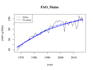
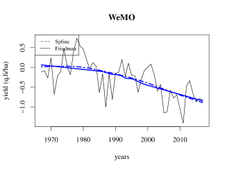
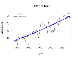
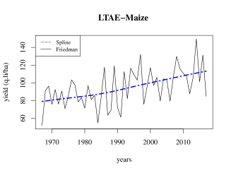
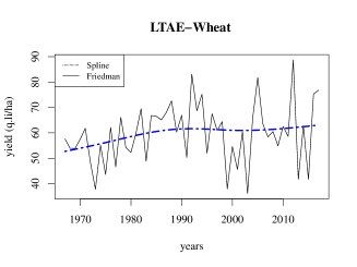
Figure 1: Time series considered in the analysis during the period 1967-2017 with computed trends.

Causality - Any causality issue has been disregarded in present analysis because of the yearly time interval of data, which make series to be assumed as synchronous [12]. SSN is an indicator of solar activity, which affects Global Circulation, that in turn affects regional climates, whose trends can be revealed by indicators as WeMO. Regional weather conditions certainly affects those of a country, whose yields aggregate those attained locally. The diagram shown in figure 2, the causality chain, displayed in figure is therefore embedded in spatial aggregation.

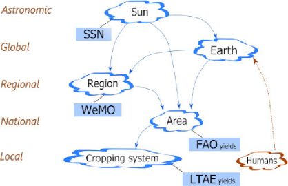
Figure 2: Relation between observed indicators and dynamical systems involved (clouds) with related scales on the left.

The diagram also shows that causality could derive from relationships between observed indicators meant as state variables of “black box” systems as Sun and General Circulation System still are. Such teleconnections are therefore embedded in observation scales.

3 Applied Method

Time Series Representation

Each time series ${x_{i}}$ is commonly represented in terms of three main components, a trend $\mu_{i}$ (sometimes decomposed into an offset-intercept and a more or less linear trend), a (more or less regular) cyclical component $y_{i}$ , and an noise $\varepsilon_{i}$ . In fact recognizing these components is strongly dependent on the method used and the hypothesis assumed. The components can be assumed to appear in an additive model, where they are independent of each other $x_{i}=\mu_{i}+y{}_{i}+\varepsilon_{i}$ (further discussed in Appendix 1).

Trend & Stationarity

Trend is in most discipline considered the most important component of time series, therefore a lot of statistical methods are oriented to model it (e.g. regression, fitting). On the other hand when signal analysis focuses on cyclical components, most of methods requires the time series be stationary (see Appendix 2), and a preliminary detrending is required. This is a common practice when having to do with time series too short to identify trend as long-time oscillation. Such a detrending is often performed by smoothing (acting like an high-pass filter) or local linear regression, as spline functions driven by a stiffness parameter, or with self-adaptation of span value [14]. First components from parametric and non-parametric methods can be also used to the purpose.

Parametric analysis

Parametric approach assumes that the signal can be represented by a family of cyclic signal are represented by a family of functions. For a continuous time signal $f(t)$, and a 1-parameter family of functions, a parameter distribution, called transform $F(\omega)$, can be obtained by the integral:

$$F(\omega)=\int_{\tau=0}^{t}K(\tau,\omega)\cdot f(\tau)\>d\tau$$ (1)

$F(\omega)$ represents the distribution of weights / amplitudes (and phases) of $K(\tau,\omega)$, the kernel of transformation. For a uniformly sampled signal $X={x_{i};i=1..N}$ transformation can be can be discretized to:

$$F_{k}=\sum_{i=1}^{N}K_{k,i}\cdot x_{i}\Longrightarrow F=K\cdot X$$ (2)

Such a linear form is the same encountered both in parametric and non-parametric approaches.

Periodical components in natural signals (astronomy, earth, living organisms) have long been studied with Fourier Analysis (FA), based on a simple harmonic $K(t,\omega)=e^{i\omega t}$, $\omega$ being the radian frequency and $t$ the observation time. Fourier Transform is applied on sampled signals by its discrete version (DFT):

$$F_{k}=\sum_{i=1}^{N}e^{i2\pi kt_{i}}\cdot x_{i}$$ (3)

where the summation is extended to a number of frequencies $k$ multiple of the sampling one and in number equal to that of the observations, $N$. To optimize computation times DFT is usually performed via the Fast Fourier Transform (FFT) requiring $N^{\prime}=2^{n}$, where $n$ are the possible frequencies.

Non-parametric analysis

Non parametric analysis is used when the signal analyst does not want or can not use pre-defined functions, and may be regarded as an extension of Functional Principal Component Analysis. To date the more diffused methods are represented by EMD and SSA. They are often considered as non-linear analysis tool, as they focus on signals hard to be generated by linear system (plane harmonics).

EMD is based on an iterative methodology called sifting: on the original (detrended) signal is identified an envelope described by a couple of curves obtained by maximum and minimum values, whose average identify the points of the so-called Intrinsic Mode Function (IMF). IMF points are used to detrend the signal, while the residual undergoes the procedure repetitively till a tolerance ($\epsilon$) is reached:

$$\sum_{t}\left(\frac{h_{j}(t)-h_{j-1}(t)}{h_{j-1}(t)}\right)^{2}<\epsilon$$ (4)

where $h_{i}(t)$ is the IMF at step $i$. Since when it has been proposed [23], IMFs have been recognized to need to be interpreted as amplitude and frequency variable functions, and Hilbert-transform (Appendix 3) has followed, allowing for obtaining a generalized Fourier expansion:

$$Y(t)=\sum_{j=1}^{n}h_{j}(t)\>e\>^{i\intop\omega_{j}(t)\>dt}$$ (5)

where $Y(t)$ is the reconstructed signal, and amplitude distribution $h_{j}(t)$ is known as Hilbert-Huang transform.

SSA allows for detecting amplitude and phase modulated oscillations [2] in terms of Empirical Orthogonal Components (EOCs). The method is based on building lagged series from the original one (of length $N$) taking $L$ records only (window size) obtaining $K\quad(=N-L-1)$ rows of the so-called trajectory matrix $T$ (embedding step). The successive $T$ is diagonalization completes the Singular Value Decomposition (SVD):

$$T=U\;D\;V^{\prime}$$ (6)

allowing to obtain the eigenvectors (diagonals of $D$), and $K$ eigenvectors of length $L$ (rows of $U$), representing the components of the signal. Components may also be collected into groups to facilitate recognition of trend, periodicity and separation of noise [18].

Non stationarity - Both parametric and non/parametric methods required the signal be stationarity together with the possibility to reconstruct the signal by a linear superposition of components.

To assess stationarity of a (detrended) signal, Kwiatkowski–Phillips–Schmidt–Shin (KPSS) test can be used to verify (HP-0) that the time series is stationary around a deterministic trend, or the (complementary) Augmented Dickey Fuller (ADF) tests (HP-0) that there is a unit root, that the characteristic equation represents an AR process (see e.g. [26]).

When the detrended signal is non-stationary, because of non-homeostaticity of the underlying system, changing frequency, phase or amplitude of signal components, the methods described above have been extended by means of local operators.

SSA has been extended for non-stationary series adding circularity in Circulant SSA (CSSA, [6]) and Sliding SSA (SSSA, [20]), which are ways to analyze locally the series by means of windows. The windowing strategy has been introduced by [15] in WFT by superimposing to the traditional kernel a windowing function $w$ :

$$K(t,to,\tau,\omega)=w(t;to,\tau)\cdot e^{i\omega t}$$ (7)

WFT allows to maintain the orthogonality of the transformation within the same interval, that is the invertibility of the Fourier transform [29]. Such an approach is also known as Short Time Fourier Transform and available by algorithms as the sliding DFT [22] well fitting the issue of having $N>N^{\prime}$, that make possible to perform the analysis on several data sets ($L=N-N^{\prime}$). Such approaches, though, do not guarantee ortho-normality . Wavelet Transform (WT) [1, 32] is identified by a two parameter convolution kernel $K(x,y)$ made of a mother wavelet $\psi(t)$, which can be interpreted as an high-pass filter, and a scaling function $\phi(t,s)$ (also called father function) which can be regarded as a low-pass filter, $s$ being the scale. Its discrete version can be written as a weighted average:

$$W_{k}(s)=\sum_{i=0}^{N-1}Q_{k,i}(s)\cdot x_{i}$$ (8)

where $Q_{i,j}=c(s)\;\psi(t_{i})\circ\phi\left(t_{i}-t_{j},s\right)=c(s)\;\psi\left((t_{i}-t_{j})/s\right)$:

Wavelet approach can adopt several mother functions, each with peculiar properties (e.g. Haar wavelet, deriving from the box function, has a real transform) that make it appropriate to certain data sets. In geophysical data it is quite used the Morlet wavelet, inheriting features of “tapering” method [39]:

$$\psi(\omega,t)=\pi^{-1/4}e^{i\omega t}e^{-t^{2}/2}$$ (9)

Wavelet technique can be used to evidence pattern superposition of two series by means of the Cross Wavelet Transform (CWT). Power spectrum $P_{k}$ definition may be extended to obtain the cross power spectrum:

$$P_{k}^{XY}=\left\langle W_{k}^{X}\;W_{k}^{Y*}\right\rangle$$ (10)

where $\left\langle\right\rangle$ stands for expected value and (^∗) for complex conjugate.

Following the scheme described above, the cumulated probability distribution of cross power spectrum for a given $p$ is :

$$D\left(\frac{\left|W_{n}^{X}(s)\;W_{n}^{Y^{*}}(s)\right|}{\sigma_{X}\;\sigma_{Y}}<p\right)=\frac{Z_{m}(p)}{m}\sqrt{P_{k}^{Y}\;P{}_{k}^{Y}}$$ (11)

where $Z(p)=\sqrt{\chi_{m}^{2}(p)\;\chi_{m}^{2}(p)}$ . As $P_{k}^{XY}$ is complex, analyzing coherency is also important, the latter being defined by:.

$$R_{k}^{2}(s)=\frac{\left|S(W_{k}^{XY}(s)/s)\right|^{2}}{S\left(\left|(W_{k}^{X}(s))\right|^{2}/s\right)\cdot S\left(\left|(W_{k}^{Y}(s))\right|^{2}/s\right)}$$ (12)

where smoothing both in scale and time is applied: $S_{k}(W_{k})=S_{time}[S_{scale}(W_{k})]$ (see [19] for details).

Denoising and Periodogram readability - In many cases noise corresponds to high frequency stationary components (2-nd order stationary), and removed applying high pass filters [3, 7].

Smoothing is also applied on periodograms (power spectrum along years), to increase their readability, and interpolated values are commonly considered consistent estimator of the true spectrum [33]. In WT (2D periodograms) things are more complex though, because neighboring points in time and scale are correlated, and expected power spectrum $P_{k}$ can be obtained from a Fourier power spectrum extending the Wiener-Khinchin theorem [33] :

$$P_{k}=\left\langle W_{k}\cdot W_{k}^{*}\right\rangle$$ (13)

where scaling factor $s$ is omitted for sake of simplicity. Applying it to a Fourier spectrum of an AR(1) $x_{t}=x_{t-1}+\alpha\cdot\varepsilon_{t}$ [2] it becomes:

$$P_{k}=\frac{1-\alpha^{2}}{1-\alpha\cdot e^{-i2\pi k}}$$ (14)

where the error $\varepsilon_{t}$ is modeled as a Gaussian model (white noise) and $\alpha$ is estimated from data. If $P_{k}$ is sufficiently smooth, the cumulated probability of a power for a given significance level $p$ is :

$$D\left(\left|W_{k}\right|^{2}<p\cdot\sigma_{k}^{2}\right)=\frac{1}{2}P_{k}\;\chi_{m}^{2}(p)$$ (15)

where $m$ is 1 for real WT (e.g.Haar) and 2 for complex ones (e.g. Morlet) [19].

Analysis steps - Starting from methods described above, many analysis recipes have been developed, and a variety of code libraries have been produced that already implement such methods in several platforms. In the present study, analysis has been carried out with RStudio (ver.1.1.456), following the steps below:

• Original signals have been formerly detrended (by $detrend.series$, package dplR, by Bunn) by ”Spline” and “Friedman” approaches, and trends are discussed.

• On detrended signals, stationarity has been successively tested by Kwiatkowski–Phillips–Schmidt–Shin (KPSS) and Augmented Dickey Fuller (ADF) test (procedures $KPSS.test$ and $ADF.test$ from package aTSA, by Debin Qiu).

• EMD (procedure $extractimf$ , package EMD, by Kim) has been used to identify noise of big amplitude which can be found in the first component (first sifting passage); on such component FFT (by $periodogram$ , package TSA, by Chan & Ripley) has been used to identify the related noise model.

• SSA has been successively performed on (by $ssa$ , package Rssa, by [24]) on EMD filtered signal to identify high frequency components corresponding to lowest eigenvalues.

• Wavelelet analysis has been performed on reconstructed signals (by $analyze.wavelet$ , package “WaveletComp”, by [37]).

• Cross Wavelelet Analysis to verify signal coherency has been finally performed by $analyze.coherency$ (package “WaveletComp”, by [37]).

4 Results

1. At a first glance (see figure 1), time series looks very different to one another. The large fluctuations visible in SSN (figure 1), corresponding to the well known $\sim 11$ year cycle (e.g. [48]), are not readily recognizable in the other series.

2. Trends by spline and Friedman techniques are very similar to one another (figure 1) and the former has been chosen for the following analysis.

3. SSN and WeMO trends looks very similar, being stable in the first decades and decreasing in the last period. A regression between the two trends ($R^{2}=0.99$) could easily suggest a strong dependence of regional climate on solar activity.

4. Strong quasi-linear trends appears especially in FAO-yield, showing the effects of the so called “green revolution” due, after the WWII, to genotype improvements and diffusion of mechanization, chemical fertilizers and pesticides. Such a rise in yield is almost reaching a plateau in Maize, still growing in Wheat. Such behavior can be explained from genetic research, which is still intensive for crops grown in dry conditions (lot of congresses and debates on drought) as wheat, whereas maize is mostly grown in irrigated areas.

5. In experimental plots (LTAE), the more stable yields of wheat with respect to maize can be ascribed to a conservative approach aimed at growing the same varieties. This want though turned to be feasible for wheat, not for maize, where seed availability is bond to crop variety commercial availability (and related patents). Moreover, despite a particular care into experimental crop management (manual weed control, fertilization management) yearly fluctuation are still large when compared to country values (FAO) which are an average of a large number of values with a variability due to different climates, cropping techniques, crop varieties,etc.

6. Stationarity tests have been performed on detrended signals (using spline method) for the base model (no drift, no trend) and results, displayed in table 1, show that SSN represents the only critical issue. Autocovariance functions are reported in appendix A2.

		SSN	WeMO	FAO-W	FAO-M	LTAE-W	LTAE-M
Spline	KPSS	>0.1	>0.1	>0.1	>0.1	>0.1	>0.1
	ADF	0.022	<0.01	<0.01	<0.01	<0.01	<0.01
Friedman	KPSS	>0.1	>0.1	>0.1	>0.1	>0.1	>0.1
	ADF	0.022	<0.01	<0.01	<0.01	<0.01	<0.01

Table 1: p values of stationarity test applied to detrended time series

As KPSS are almost every time > 0.1 and ADF values < 0.05 detrended data can be considered stationary.

In figure 3 the detrended signals are shown together with the signal reconstructed from EMD excluding the first component, whose FFT is shown on the right.

Figure 3: EMD-based noise identification

This was not possible for SSN where first component incorporates the main oscillation, how it is evidenced from FFT. SSN and WeMO preliminary annual average seems in fact to be sufficient to filter out higher frequencies in the first, being much less effective in the second, so that the first component of EMD is still significantly high.

A similar procedure has been performed by SSA, to identify low amplitude noise components with the aid of eigenvalues distribution (left plot in figure 4); the same figure reports denoized signals together with the filtered noise.

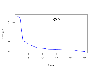
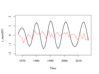
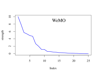
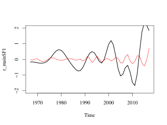
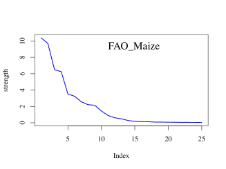
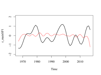
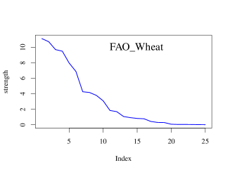
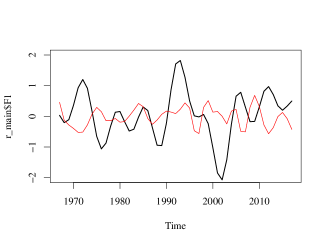
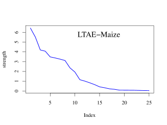
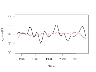
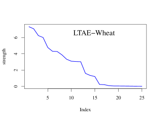
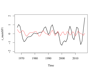
Figure 4: SSA-based noise identification

On detrended signals, the WA allows to locate frequencies in different time domains making things more readable (figure 5). In the periodograms it is possible to notice an arc-shaped region, which reflects the interval of validity of wavelet analysis: the greater is the period, the narrow is the interval of data (year window). Black and white lines represent 90% and 95% confidence limits of the power values (see side bar).

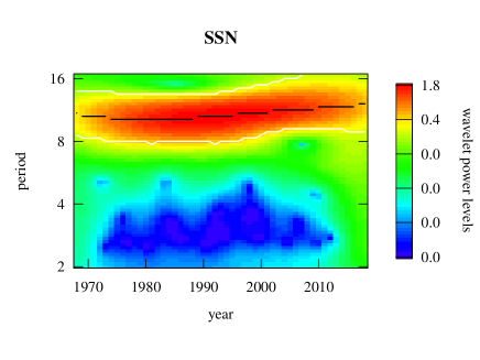
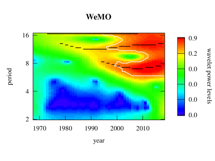
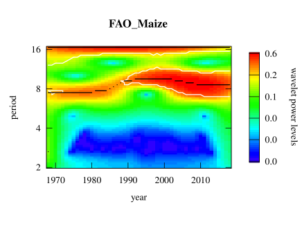
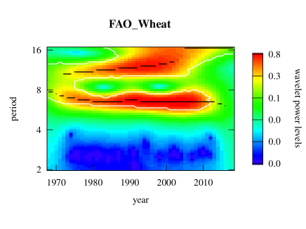
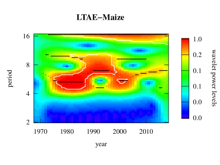
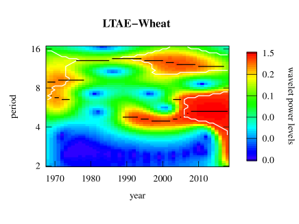
Figure 5: Wavelet transform of detrended normalized EMD-denoised series

From figure it is quite evident a shift in frequency moving from the 11 years of 1970-2000 to higher values in the last two decades. More evident is in WeMO the passage from a rather quiescent zone (small amplitude fluctuations) of the first 3 decades to oscillations within the range of 7-16 years for the last two decades. Such a behavior can be slightly recognized in FAO-Maise, wheres FAO-Wheat slower oscillations seems to follow more SSN, apart of a more rapid fluctuation around 7 years which seems to disappear in the last decade. Fluctuations in LTAE-Maize with a period of 5-9 years evident in 1980-2000, whereas in LTAE-Wheat strong fluctuations around 4-7 years are appearing in the last two decades.

Other suggestions are searched with the help of cross-wavelet analysis, which put in evidence how SSN 11-year fluctuation and its shift can be detected in almost every other signals. Also WeMO increase of fluctuation with a large spectrum (4-16 years) seems to affect yield both at a national and local scale.

More difficult is interpreting spectrogram related to comparison of yield fluctuations, though those of maize seems to be more concentrated in the past (central decades) while those of wheat seem to increase in the last decade.

	SSN	WeMO	FAO-Maize	FAO-Wheat	LTAE-Maize
WeMO
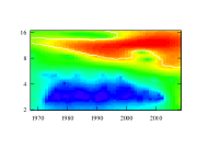
FAO-Maize
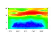
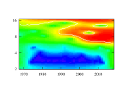
FAO-Wheat
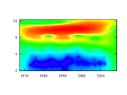
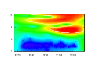
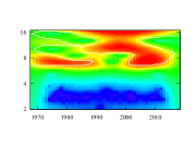
LTAE-Maize
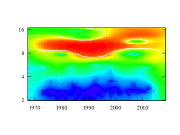
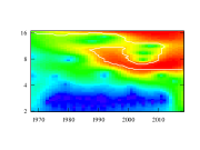
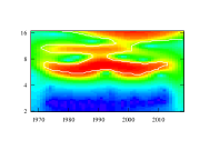
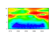
LTAE-Wheat

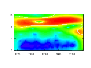
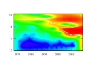
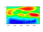
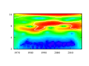
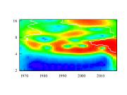
Figure 6: Cross Wavelet Transform of detrended, normalised and EMD-denoised reconstructed series. In the second column the lower frequency have been dumped to mask the effect of SSN.

Conclusions

The aim of this study is to investigate how climate change affects yields of major crops as maize and wheat, focusing on trends and fluctuations, useful to estimate production forecasts and related risks.

The analysis investigates possible relations of local yields with national ones, a classical regional climatic index as Western Mediterranean Oscillation Index, and a global one given by Sun Spot Number.

The present investigation shows how SSN oscillations affects regional scale dynamics, recorded by indicators as WeMO, which in turn reflects on the yield of Wheat and Maize.

The analysis suffered the a small size of time series (51 years) though non-parametric methods as EMD and SSA seemed efficient in identifying and remove noise components.

On the back of any derived conclusions there is the analysis some historical series of climate indicators, whose causal connections are not jet clearly perceivable to important stakeholders as the farmer.

Another consideration regards the number of years requested to obtain a view of a significant trend in climatic conditions that influence crop yield. It seems that both at a global level and locally, the annual anomalies around an average are so wide that a clear trend, even if significant, needs a high number of years to be perceived. During the lifespan of a farmer he would be hardly understand if our planet is going toward a colder or a hotter end. Therefore he has not any mean, based only on his experience, to decide if it’s better to change is production system in a way or another.

Such connections, having an empathized impact on communication media, citizen, stakeholders and decision makers, are based on indicators and variables related to measured variables, but often far from common perception: this is the case of El-Nino Souther Oscillation index, which long has been related to astronomical components [4], both far from real world experience.

Understanding such fluctuations is of strategic importance not only for economy of commodities, but also concerning food security. The agro-environmental system is characterized by variables reflecting the behavior of complex dynamics that cannot be ascribed to specific causes. Recently many researches are addressing the climate change issue, trying to identify and confirm the reasons at the base of the many expected (not always tangible), effects of such environmental drift on human life. Though most of the studies focus on food security, an analysis of the real effects of climate change on crop production is still lacking.

Finally it has to be put in evidence the importance of Long Term Agronomic Experiments. While the trend of the average Italian temperatures and annual rainfall can be obtained for a long period [30], yields are less reconstructable [9]. Therefore they represent a source of data that, though influenced by soil type and technical management, it embeds long-range seasonality.

Finally, to avoid any manipulation of present results, authors want to underline that the effects of human activities on climate change is not discussed in this work.

Appendix 1 - Time Series Analysis

Instead of additive model, multiplicative, $x_{i}=\mu_{i}\times y{}_{i}\times\varepsilon_{i}$ or mixed ones (e.g. $x_{i}=\mu_{i}\times\varepsilon_{i}+y_{i}$) can be adopted emerging from a Time Series Analysis, where observations are used to develop a mathematical model which captures the underlying Data Generation Process (DGP), which could be extremely useful for predictions. A common strategy is interpreting a time series ${x(t)}$ as a realization of a stochastic process, a sample of the totality of realizations which is called ensemble. Such a sample can be used to estimate the joint probability distribution of the random variable involved, describing the probability structure of the time series as a stochastic process.

Most of time series analysis relay on linearity assumption, meaning that it can be modeled by a linear stochastic process, where the current value of the series is a linear function of past observations.

Linear processes include AutoRegressive (AR) model, Moving Average (MA) and derived ones (ARMA, ARIMA, SARIMA, Box-Jenkins):

$$AR) x(t)=\mu+\varepsilon(t)+\sum_{j=1}^{p}\alpha_{j}\cdot x(t-j)$$

$$MA) x(t)=\mu+\varepsilon(t)+\sum_{j=1}^{q}\beta_{j}\cdot\varepsilon(t-j)$$

$$ARMA) x(t)=\mu+\varepsilon(t)+\sum_{j=1}^{p}\alpha_{j}\cdot x(t-j)+\sum_{j=1}^{q}\beta_{j}\cdot\varepsilon(t-j)$$

$$ARIMA_{1}) x(t)=\varepsilon(t)+\sum_{j=1}^{p}\alpha_{j}\cdot x(t-j)-\sum_{j=1}^{q}\beta_{j}\cdot\varepsilon(t-j)$$

where $p$ is the lag order for AR model, $\alpha_{j}$ representing the weight/memory of past observations $x(t-j)$, $q$ is the order of moving average, $\beta_{j}$ representing the weights over past forecast (non observed) errors $\varepsilon(t-j)$. While ARMA is just a simple combination of the two, ARIMA is based on differentiating (in the reported equation the degree of differentiating d=1).

Linearity may be tested by a number of methods ([5], all of them lay on surrogate data generation [38],[27]) as Teraesvirta’s and White’s test (based on neural network), verifying HP0: “Linearity in mean", Keenan’s, Tsay’s and likelihood’s tests, with HP0: “The time series is generated from a Non-Linear AR process”, McLeod-Li’s test for Heteroschedasticity with HP0: “The time series is generated from a Non-Linear ARIMA process”. Such test are based on quasi-stationarity of time series.

Table 2 show the results of linearity test performed with 6 different methods mentioned above on spline detrended data.

	test	SSN	WeMO	FAO-W	FAO-M	LTAE-W	LTAE-M
linearity in ’mean’	Teraesvirta	0.618	0.202	0.069	0.125	0.741	0.282
	White	0.581	0.195	0.164	0.100	0.640	0.322
NL-AR	Keenan	0.228	0.883	0.099	0.932	0.703	0.117
	Tsay	0.022	0.041	0.044	0.386	0.732	0.003
	likelihood	$1e^{-7}$	0.430	0.061	0.257	0.334	0.003
NL-ARIMA	McLeod-Li	0.014	1.000	0.557	0.979	0.585	0.791

Table 2: p-values of stability test applied on detrended time series

From table 2 we can see that null hypothesis (linearity in ’mean’) can be accepted in the majority of cases, with the exceptions for FAO-W emerging from Teraesvirta test. However there are also strong clues on non-linearity, after Keenan’s test in every series, which are confirmed by every test on FAO-M and LTAE-W.

Appendix 2 - Stationarity and ACF

Stationarity is a property making the time series useful for forecasts, which could be meant in several ways. Strict stationarity, wanting $X={x_{i}}={x_{i+h}}$ for every $h$ is hardly used; first order stationarity requires a constant local average $E(X_{t})$, being $X_{t}$ is a subset of original series around $t$; finally the second order or weak stationarity requires a constant variance $\sigma^{2}(X_{t})$ and an Auto Correlation Function (ACF) not depending on time. The latter is the one commonly adopted.

Being ACF:

$$\rho_{k}=cov(X,X_{k})/\left(Var(X)\cdot Var(X_{k})\right)$$ (16)

where $X_{k}$ is the series shifted of a time lag $k$, in stationary conditions it reduces to:

$$\rho_{k}=cov(X,X_{k})/\sigma^{2}$$ (17)

ACF allows to reveal both the presence of a trend and to spot periodical components.

For the adopted time series, ACF can be seen in the figure BELOW

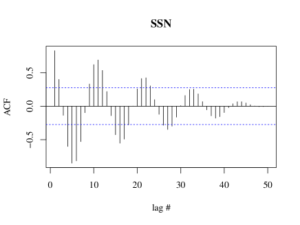
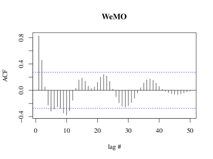
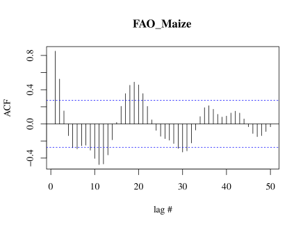
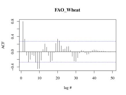
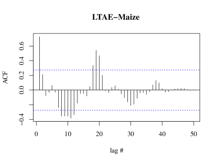
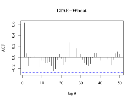
Figure 7: Autocovariance functions for time series, showing a clear decrease in SSN and WeMO in the last decades.

References

- [1] Paul Addison. The Illustrated Wavelet Transform Handbook. Taylor & Francis, jul 2002.
- [2] Myles R. Allen, Leonard A. Smith, Myles R. Allen, and Leonard A. Smith. Monte Carlo SSA: Detecting irregular oscillations in the Presence of Colored Noise. Journal of Climate, 9(12):3373–3404, dec 1996.
- [3] A. M. Alvarez-Meza, C. D. Acosta-Medina, and G. Castellanos-Dominguez. Automatic singular spectrum analysis for time-series decomposition. ESANN 2013 proceedings, 21st European Symposium on Artificial Neural Networks, Computational Intelligence and Machine Learning, (April):131–136, 2013.
- [4] M. R. Attolini, S. Cecchini, M. Galli, and T. Nanni. On the persistence of the 22 y solar cycle. Solar Physics, 125(2):389–398, 1990.
- [5] Luisa Bisaglia and Margherita Gerolimetto. Testing for (non)linearity in economic time series: a Montecarlo comparison, 2014.
- [6] Juan Bógalo, Pilar Poncela, and Eva Senra. Automatic Signal Extraction for Stationary and Non-Stationary Time Series by Circulant SSA, 2017.
- [7] Abdel-O. Boudraa, Jean-Christophe Cexus, and Zazia Saidi. EMD-Based Signal Noise Reduction. Signal Processing, pages 33–37, 2005.
- [8] Andreas Bruns. Fourier-, Hilbert- and wavelet-based signal analysis: are they really different approaches? Journal of Neuroscience Methods, 137(2):321–332, aug 2004.
- [9] L. Cavazza. Aspetti agronomici della produzione foraggera nel Mezzogiorno. In Atti di "Strutture e Mercati dell’Agricoltura Meridionale", 6 Carni, Tomo I, 1-273. Ed.Cassa per il Mezzogiorno, Roma, 1966.
- [10] Frédéric Clette, Leif Svalgaard, José M. Vaquero, and Edward W. Cliver. Revisiting the Sunspot Number. Space Science Reviews, 186(1-4):35–103, dec 2014.
- [11] Patrick Matthew Crowley. An intuitive guide to wavelets for economists. jan 2005.
- [12] Neville Davies and C. Chatfield. The Analysis of Time Series: An Introduction. The Mathematical Gazette, 74(468):194, jun 1990.
- [13] C. de Jager and H. Nieuwenhuijzen. Terrestrial ground temperature variations in relation to solar magnetic variability, including the present Schwabe cycle. Natural Science, 05(10):1112–1120, sep 2013.
- [14] J. H. Friedman. A variable span smoother. Technical report, Laboratory for Computational Statis-tics,Department of Statistics,, 1984.
- [15] D. Gabor. Theory of communication. Part 1: The analysis of information. Journal of the Institution of Electrical Engineers - Part III: Radio and Communication Engineering, 93(26):429–441, nov 1946.
- [16] H. C. J. Godfray, J. R. Beddington, I. R. Crute, L. Haddad, D. Lawrence, J. F. Muir, J. Pretty, S. Robinson, S. M. Thomas, and C. Toulmin. Food Security: The Challenge of Feeding 9 Billion People. Science, 327(5967):812–818, feb 2010.
- [17] Nina Golyandina, A Shlemov arXiv preprint ArXiv:1308.4022, Undefined 2013, and Alex Shlemov. Variations of singular spectrum analysis for separability improvement: non-orthogonal decompositions of time series. arxiv.org, aug 2013.
- [18] Nina Golyandina and Anton Korobeynikov. Basic Singular Spectrum Analysis and Forecasting with R. Computational Statistics and Data Analysis, 71:934–954, 2014.
- [19] A. Grinsted, J. C. Moore, and S. Jevrejeva. Application of the cross wavelet transform and wavelet coherence to geophysical time series. Nonlinear Processes in Geophysics, 11(5/6):561–566, nov 2004.
- [20] Jinane Harmouche, Dominique Fourer, Francois Auger, Pierre Borgnat, and Patrick Flandrin. The Sliding Singular Spectrum Analysis: A Data-Driven Nonstationary Signal Decomposition Tool. IEEE Transactions on Signal Processing, 66(1):251–263, jan 2018.
- [21] Virden L. Harrison. Do Sunspot Cycles Affect Crop Yields ? Technical report, ECONOMIC RESEARCH SERVICE U.S. DEPARTMENT OF AGRICULTURE, 1974.
- [22] Gerhard Heinzel, Albrecht Rüdiger, and Roland Schilling. Spectrum and spectral density estimation by the Discrete Fourier transform (DFT), including a comprehensive list of window functions and some new at-top windows. 2002.
- [23] Norden E. Huang, Zheng Shen, Steven R. Long, Manli C. Wu, Hsing H. Shih, Quanan Zheng, Nai-Chyuan Yen, Chi Chao Tung, and Henry H. Liu. The empirical mode decomposition and the Hilbert spectrum for nonlinear and non-stationary time series analysis. Proceedings of the Royal Society of London. Series A: Mathematical, Physical and Engineering Sciences, 454(1971):903–995, mar 1998.
- [24] Anton Korobeynikov. Computation- and space-efficient implementation of SSA. Statistics and Its Interface, 3(3):357–368, nov 2010.
- [25] B. Kozlowski. Weather Indicators and Crop Yields Analysis with Wavelets. Technical report, IIASA Interim Report, 2007.
- [26] Denis Kwiatkowski, Peter C. B. Phillips, Peter Schmidt, and Yongcheol Shin. Testing the null hypothesis of stationarity against the alternative of a unit root: How sure are we that economic time series have a unit root? Journal of Econometrics, 54(1-3):159–178, 1992.
- [27] Gemma Lancaster, Dmytro Iatsenko, Aleksandra Pidde, Valentina Ticcinelli, and Aneta Stefanovska. Surrogate data for hypothesis testing of physical systems. Physics Reports, 748:1–60, jul 2018.
- [28] David B. Lobell and Marshall B. Burke. On the use of statistical models to predict crop yield responses to climate change. Agricultural and Forest Meteorology, 150(11):1443–1452, oct 2010.
- [29] Alfred Karl Louis, P. Maass, and A. (Andreas) Rieder. Wavelets : theory and applications. Wiley, 1997.
- [30] Galli M. Time series analysis with power spectrum and cyclograms, Solar-terrestrial relationships and the earth environment in the last millennia. In SIF 1988, pages 246–273, 1988.
- [31] M. D. Mahecha, M. Reichstein, H. Lange, N. Carvalhais, C. Bernhofer, T. Grünwald, D. Papale, and G. Seufert. Characterizing ecosystem-atmosphere interactions from short to interannual time scales. Biogeosciences, 4(5):743–758, sep 2007.
- [32] Stéphane G. Mallat and Gabriel Peyré. A wavelet tour of signal processing : the sparse way. Elsevier/Academic Press, 2009.
- [33] D. Maraun and J. Kurths. Cross wavelet analysis: significance testing and pitfalls. Nonlinear Processes in Geophysics, 11(4):505–514, nov 2004.
- [34] James Ramsay and B. W. Silverman. Functional Data Analysis. Springer-Verlag, New York, 2005.
- [35] Deepak K. Ray, Paul C. West, Michael Clark, James S. Gerber, Alexander V. Prishchepov, and Snigdhansu Chatterjee. Climate change has likely already affected global food production. PLOS ONE, 14(5):e0217148, may 2019.
- [36] E.A. Robinson. Physical Applications of Stationary Time-Series. Charles Griffith & Co.Ltd., 1980.
- [37] A. Roesch and H. Schmidbauer. Package "WaveletComp". Technical report, 2018.
- [38] James Theiler, Stephen Eubank, André Longtin, Bryan Galdrikian, and J. Doyne Farmer. Testing for nonlinearity in time series: the method of surrogate data. Physica D: Nonlinear Phenomena, 58(1-4):77–94, sep 1992.
- [39] D.J. Thomson. Spectrum estimation and harmonic analysis. In Proceedings of the IEEE, 1982.
- [40] L. Triberti, A. Nastri, and G. Baldoni. Long-term effects of crop rotation, manure and mineral fertilisation on carbon sequestration and soil fertility. European journal of Agronomy, 74:47–55, 2016.
- [41] B. Usowicz and J.B. Usowicz. Spatial and temporal variation of selected physical and chemical properties of soil. Technical report, 2004.
- [42] Laura Uusitalo, Annukka Lehikoinen, Inari Helle, and Kai Myrberg. Environmental modelling & software : with environment data news. Elsevier Science Ltd, 2015.
- [43] R. Vautard and M. Ghil. Singular spectrum analysis in nonlinear dynamics, with applications to paleoclimatic time series. Physica D: Nonlinear Phenomena, 35(3):395–424, may 1989.
- [44] F. Vercelli. Analisi Periodale. Tecnica Italiana, (Anno IX, N.2):12, 1954.
- [45] Juan Manuel Vilar, José Antonio Vilar, and Sonia Pértega. Classifying Time Series Data: A Nonparametric Approach. Journal of Classification, 26(1):3–28, apr 2009.
- [46] G. Vitali. La trasformata wavelets nell’interpretazione agro-climatologica. In SIA 1999, 1999.
- [47] Keith Wiebe, Hermann Lotze-Campen, Ronald Sands, Andrzej Tabeau, Dominique van der Mensbrugghe, Anne Biewald, Benjamin Bodirsky, Shahnila Islam, Aikaterini Kavallari, Daniel Mason-D’Croz, Christoph Müller, Alexander Popp, Richard Robertson, Sherman Robinson, Hans van Meijl, and Dirk Willenbockel. Climate change impacts on agriculture in 2050 under a range of plausible socioeconomic and emissions scenarios. Environmental Research Letters, 10(8):085010, aug 2015.
- [48] RuoWen Yang, Jie Cao, Wei Huang, and AiBing Nian. Cross wavelet analysis of the relationship between total solar irradiance and sunspot number. Chinese Science Bulletin, 55(20):2126–2130, jul 2010.
Acknowledgments
Authors are thankful to “World Data Center for the production, preservation and dissemination of the international sunspot number”, the “Climatic Research Unit of East Anglia University” for Western Mediterranean Oscillation index records availability, FAO for data dissemination efforts, and R, R-Studio developers and contributors for allowing and maintain free access to their products.