Variance Reduced Coordinate Descent with Acceleration:
New Method With a Surprising Application to Finite-Sum Problems

Abstract

We propose an accelerated version of stochastic variance reduced coordinate descent – ASVRCD. As other variance reduced coordinate descent methods such as SEGA or SVRCD, our method can deal with problems that include a non-separable and non-smooth regularizer, while accessing a random block of partial derivatives in each iteration only. However, ASVRCD incorporates Nesterov’s momentum, which offers favorable iteration complexity guarantees over both SEGA and SVRCD. As a by-product of our theory, we show that a variant of Katyusha [1] is a specific case of ASVRCD, recovering the optimal oracle complexity for the finite sum objective.

1 Introduction

In this paper, we aim to solve the regularized optimization problem

$$\min_{x\in\mathbb{R}^{d}}P(x):=f(x)+\psi(x),$$ (1)

where function $f$ is convex and differentiable, while the regularizer $\psi$ is convex and non-smooth. Furthermore, we assume that the dimensionality $d$ is large.

The most standard approach to deal with the huge $d$ is to decompose the space, i.e., use coordinate descent, or, more generally, subspace descent methods [24, 37, 19]. Those methods are especially popular as they achieve a linear convergence rate on strongly convex problems while enjoying a relatively cheap cost of performing each iteration.

However, coordinate descent methods are only feasible if the regularizer $\psi$ is separable [31]. In contrast, if $\psi$ is not separable, the corresponding stochastic gradient estimator has an inherent (non-zero) variance at the optimum, and thus the linear convergence rate is not achievable.

This phenomenon is, to some extent, similar when applying Stochastic Gradient Descent (SGD) [32, 23] on finite sum objective – the corresponding stochastic gradient estimator has a (non-zero) variance at the optimum, which prevents SGD from converging linearly. Recently, the issue of sublinear convergence of SGD has been resolved using the idea of control variates [14], resulting in famous variance reduced methods such as SVRG [16] and SAGA [5].

Motivated by the massive success of variance reduced methods for finite sums, control variates have been proposed to “fix” coordinate descent methods to minimize problem (1) with non-separable $\psi$. To best of our knowledge, there are two such algorithms in the literature – SEGA [11] and SVRCD [13], which we now quickly describe.

Let $x^{k}$ be the current iterate of SEGA (or SVRCD) and suppose that the oracle reveals $\nabla_{i}f(x^{k})$ (for $i$ chosen uniformly at random). The simplest unbiased gradient estimator of $\nabla f(x^{k})$ can be constructed as $\tilde{g}^{k}=d\nabla_{i}f(x^{k})e_{i}$ (where $e_{i}\in\mathbb{R}^{d}$ is the $i$-th standard basis vector). The idea behind these methods is to enrich $\tilde{g}^{k}$ using a control variate $h^{k}\in\mathbb{R}^{d}$, resulting in a new (still unbiased) gradient estimator $g^{k}$:

$$g^{k}=d\nabla_{i}f(x^{k})e_{i}-dh_{i}^{k}e_{i}+h^{k}.$$

How to choose the sequence of control variates $\{h^{k}\}$? Intuitively, we wish for both sequences $\{h^{k}\}$ and $\{\nabla f(x^{k}\})$ to have an identical limit point. In such case, we have $\lim_{k\rightarrow\infty}\mathrm{Var}(g^{k})=0$, and thus one shall expect faster convergence. There is no unique way of setting $\{h^{k}\}$ to have the mentioned property satisfied – this is where SEGA and SVRCD differ. See Algorithm 1 for details.

Algorithm 1 SEGA and SVRCD

0:  Stepsize $\alpha>0$, starting point $x^{0}\in\mathbb{R}^{d}$, probability vector $p$: $p_{i}\coloneqq\mathbb{P}\left(i\in S\right)$

  Set $h^{0}=0\in\mathbb{R}^{d}$

  for  $k=0,1,2,\ldots$  do

     Sample random $S\subseteq\{1,2,\dots,d\}$

     $g^{k}=\sum\limits_{i\in S}\frac{1}{{\color[rgb]{0,0,0}p_{i}}}(\nabla_{i}f(x^{k})-h_{i}^{k}){\color[rgb]{0,0,0}e_{i}}+h^{k}$

     $x^{k+1}=\mathop{\mathrm{prox}}\nolimits_{\alpha\psi}(x^{k}-\alpha g^{k})$

     $h^{k+1}=\begin{cases}h^{k}+\sum\limits_{i\in S}(\nabla_{i}f(x^{k})-h^{k}_{i}){\color[rgb]{0,0,0}e_{i}}&\text{for SEGA}\\ \begin{cases}\nabla f(x^{k})&\text{w.p. }{\color[rgb]{0,0,0}\rho}\\ h^{k}&\text{w.p. }1-{\color[rgb]{0,0,0}\rho}\end{cases}&\text{for SVRCD}\end{cases}$

  end for

In this work, we continue the above research along the lines of variance reduced coordinate descent algorithms, with surprising consequences.

1.1 Contributions

Here we list the main contributions of this paper.

$\triangleright$ Exploiting prox in SEGA/SVRCD. Assume that the regularizer $\psi$ includes an indicator function of some affine subspace of $\mathbb{R}^{d}$. We show that both SEGA and SVRCD might exploit this fact, resulting in a faster convergence rate. As a byproduct, we establish the same result in the more general framework from [13] (presented in the appendix).

$\triangleright$ Accelerated SVRCD. We propose an accelerated version of SVRCD - ASVRCD. ASVRCD is the first accelerated variance reduced coordinate descent to minimize objectives with non-separable, proximable regularizer.

$\triangleright$ SEGA/SVRCD/ASCRVD generalizes SAGA/L-SVRG/L-Katyusha. We show a surprising link between SEGA and SAGA. In particular, SAGA is a special case of SEGA; and the new rate we obtain for SEGA recovers the tight complexity of SAGA [29, 8]. Similarly, we recover loopless SVRG (L-SVRG) [15, 18] along with its best-known rate [13, 28] using a result for SVRCD. Lastly, as a particular case of ASVRCD, we recover an algorithm which is marginally preferable to loopless Katyusha (L-Katyusha) [28]: while we recover their iteration complexity result, our proof is more straightforward, and at the same time, the stepsize for the proximal operator is smaller.

1.2 Preliminaries

As mentioned in Section 1.1, the new results we provide i are particularly interesting if the regularizer $\psi$ contains an indicator function of some affine subspace of $\mathbb{R}^{d}$.

Assumption 1.1

Assume that ${\color[rgb]{0,0,0}}$ is a projection matrix such that

$$\psi(x)=\begin{cases}\psi^{\prime}(x)&{\text{i}f}\quad x\in\{x^{0}+{\rm Range}\left({\color[rgb]{0,0,0}}\right)\}\\ \infty&{\text{i}f}\quad x\not\in\{x^{0}+{\rm Range}\left({\color[rgb]{0,0,0}}\right)\}\end{cases}$$ (2)

for some convex function $\psi^{\prime}(x)$. Furthermore, suppose that the proximal operator of $\psi$ is cheap to compute.

Remark 1.1

If $\psi$ is convex, there is always some ${\color[rgb]{0,0,0}}$ such that (2) holds as one might choose ${\color[rgb]{0,0,0}}={\bf I}$.

Next, we require smoothness of the objective, as well as the strong convexity over the affine subspace given by ${\rm Range}\left({\color[rgb]{0,0,0}}\right)$.

Assumption 1.2

Function $f$ is ${\bf M}$-smooth, i.e., for all $x,y\in\mathbb{R}^{d}$:

$$f(x)\leq f(y)+\langle\nabla f(y),x-y\rangle+\frac{1}{2}\|x-y\|^{2}_{{\bf M}}.$$

Function $f$ is $\mu$-strongly convex over $\{x^{0}+{\rm Range}\left({\color[rgb]{0,0,0}}\right)\}$, i.e., for all $x,y\in\{x^{0}+{\rm Range}\left({\color[rgb]{0,0,0}}\right)\}$:

$$f(x) \geq f(y)+\langle\nabla f(y),x-y\rangle+\frac{\mu}{2}\|x-y\|^{2}.$$ (3)

Remark 1.2

Smoothness with respect to matrix ${\bf M}$ arises naturally in various applications. For example, if $f(x)=f^{\prime}({\bf A}x)$, where $f^{\prime}$ is $L^{\prime}$-smooth (for scalar $L^{\prime}>0$), we can derive that $f$ is ${\bf M}=L^{\prime}{\bf A}^{\top}{\bf A}$-smooth.

In order to stress the distinction between the finite sum setup and the setup from the rest of the paper, we are denoting the finite-sum variables that differ from the non-finite sum case in red. We thus, recommend printing this paper in color.

2 Better rates for SEGA and SVRCD

In this section, we show that a specific structure of nonsmooth function $\psi$ might lead to faster convergence of SEGA and SVRCD.

The next lemma is a direct consequence of Assumption 1.1 – it shows that proximal operator of $\psi$ is contractive under ${\color[rgb]{0,0,0}}$-norm.

Lemma 2.1

Let $\{x^{k}\}_{k\geq 0}$ be a sequence of iterates of Algorithm 1 and let $x^{*}$ be optimal solution of (1). Then

$$x^{k}\in\{x^{0}+{\rm Range}\left({\color[rgb]{0,0,0}}\right)\},\;x^{*}\in\{x^{0}+{\rm Range}\left({\color[rgb]{0,0,0}})\right)\}.$$ (4)

for all $k$. Furthermore, for any $x,y\in\mathbb{R}^{d}$ we have

$$\|\mathop{\mathrm{prox}}\nolimits_{\alpha\psi}(x)-\mathop{\mathrm{prox}}\nolimits_{\alpha\psi}(y)\|^{2}\leq\|x-y\|^{2}_{{\color[rgb]{0,0,0}}}.$$ (5)

Next, we state the convergence rate of both SEGA and SVRCD under Assumption 1.1 as Theorem 2.2. We also generalize the main theorem from [13] (fairly general algorithm which covers SAGA, SVRG, SEGA, SVRCD, and more as a special case; see Section E of the appendix); from which the convergence rate of SEGA/SVRCD follows as a special case.

Theorem 2.2

Let Assumptions 1.1, 1.2 hold and denote $p_{i}\coloneqq\mathbb{P}\left(i\in S\right)$. Consider vector $v=\sum_{i=1}^{d}{\color[rgb]{0,0,0}e_{i}}v_{i},v_{i}\geq 0$ such that

$${\bf M}^{\frac{1}{2}}\mathbb{E}\left[\sum_{i\in S}\frac{1}{{\color[rgb]{0,0,0}p_{i}}}{\color[rgb]{0,0,0}e_{i}}{\color[rgb]{0,0,0}e_{i}}^{\top}{\color[rgb]{0,0,0}}\sum_{i\in S}\frac{1}{{\color[rgb]{0,0,0}p_{i}}}{\color[rgb]{0,0,0}e_{i}}{\color[rgb]{0,0,0}e_{i}}^{\top}\right]{\bf M}^{\frac{1}{2}}\preceq{\bf D}(p^{-1}\circ v),$$ (6)

where ${\bf D}(\cdot)$ is a diagonal operator. Then, iteration complexity of SEGA with $\alpha=\min_{i}\frac{{\color[rgb]{0,0,0}p_{i}}}{4v_{i}+\mu}$ is $\max_{i}\left(\frac{4v_{i}+\mu}{{\color[rgb]{0,0,0}p_{i}}\mu}\right)\log\frac{1}{\epsilon}$. At the same time, iteration complexity of SVRCD with $\alpha=\min_{i}\frac{1}{4v_{i}{\color[rgb]{0,0,0}p_{i}}^{-1}+\mu{\color[rgb]{0,0,0}\rho}^{-1}}$ is $\left(\frac{4\max_{i}(v_{i}{\color[rgb]{0,0,0}p_{i}}^{-1})+\mu{\color[rgb]{0,0,0}\rho}^{-1}}{\mu}\right)\log\frac{1}{\epsilon}$.

Let us look closer to convergence rate of SVRCD from Theorem 2.2. The optimal vector $v$ is a solution to the following optimization problem

$$\min_{v\in\mathbb{R}^{d}}\;\;\left(\frac{4\max_{i}\{v_{i}{\color[rgb]{0,0,0}p_{i}}^{-1}\}+\mu{\color[rgb]{0,0,0}\rho}^{-1}}{\mu}\right)\log\frac{1}{\epsilon}\;\;\text{s. t.}\;\eqref{eq:ESO_sega_good}\;\text{holds}.$$

Clearly, there exists a solution of the form $v\propto p$; let us thus choose $v\coloneqq{\cal L}p$ with ${\cal L}>0$. In this case, to satisfy (6) we must have

$${\cal L}=\lambda_{\max}\left({\bf M}^{\frac{1}{2}}\mathbb{E}\left[\sum_{i\in S}\frac{1}{{\color[rgb]{0,0,0}p_{i}}}{\color[rgb]{0,0,0}e_{i}}{\color[rgb]{0,0,0}e_{i}}^{\top}{\color[rgb]{0,0,0}}\sum_{i\in S}\frac{1}{{\color[rgb]{0,0,0}p_{i}}}{\color[rgb]{0,0,0}e_{i}}{\color[rgb]{0,0,0}e_{i}}^{\top}\right]{\bf M}^{\frac{1}{2}}\right)$$ (7)

and the iteration complexity of SVRCD becomes $\left(\frac{4{\cal L}+\mu{\color[rgb]{0,0,0}\rho}^{-1}}{\mu}\right)\log\frac{1}{\epsilon}$.

How does ${\color[rgb]{0,0,0}}$ influence the rate? As mentioned, one can always consider ${\color[rgb]{0,0,0}}={\bf I}$. In such a case, we recover the convergence rate of SEGA and SVRCD from [13]. However, the smaller rank of ${\color[rgb]{0,0,0}}$ is, the faster rate is Theorem 2.2 providing. To see this, it suffices to realize that if ${\cal L}$ is increasing in ${\color[rgb]{0,0,0}}$ (in terms of Loewner ordering).

Example 2.3

Let ${\bf M}={\bf I}$ and $S=\{i\}$ with probability $d^{-1}$ for all $1\leq i\leq d$. Given that ${\color[rgb]{0,0,0}}={\bf I}$, it is easy to see that ${\cal L}=d$. In such case, the iteration complexity of SVRCD is $\left(\frac{4d+\mu{\color[rgb]{0,0,0}\rho}^{-1}}{\mu}\right)\log\frac{1}{\epsilon}$. In the other extreme, if ${\color[rgb]{0,0,0}}=\frac{1}{d}ee^{\top}$, we have ${\cal L}=1$, which yields complexity (of SVRCD) $\left(\frac{4+\mu{\color[rgb]{0,0,0}\rho}^{-1}}{\mu}\right)\log\frac{1}{\epsilon}$. Therefore, given that $\mu={\cal O}({\color[rgb]{0,0,0}\rho})$, the low rank of ${\color[rgb]{0,0,0}}$ caused the speedup of order $\Theta(d)$.

We shall also note that the tight rate of SAGA and L-SVRG might be recovered from Theorem 2.2 only using a non-trivial ${\color[rgb]{0,0,0}}$ (see Section 3), while the original theory of SEGA and SVRCD only yield a suboptimal rate for both SAGA and L-SVRG.

Connection with Subspace SEGA [11].

Assume that function $f$ is of structure $f(x)=h({\bf A}x)$. As a consequence, we have $\nabla f(x)={\bf A}^{\top}\nabla h({\bf A}x)$ and thus $\nabla f(x)\in{\rm Range}\left({\bf A}^{\top}\right)$. This fact was exploited by Subspace SEGA in order to achieve a faster convergence rate. Our results can mimic Subspace SEGA by setting $\psi$ to be an indicator function of $x^{0}+{\rm Range}\left({\bf A}^{\top}\right)$, given that there is no extra non-smooth term in the objective.

Remark 2.4

Throughout all proofs of this section, we have used a weaker conditions than Assumption 1.2. In particular, instead of-${\bf M}$-smoothness, it is sufficient to have $D_{f}(x,x^{*})\geq\frac{1}{2}\left\|\nabla f(x)-\nabla f(x^{*})\right\|^{2}_{{\bf M}^{-1}}$ for all $x\in\mathbb{R}^{d}$ (Lemma E.3 shows that it is indeed a consequence of ${\bf M}$ smoothness and convexity). At the same time, instead of $\mu$-strong convexity, it is sufficient to have $\mu$-quasi strong convexity, i.e., for all $x\in\{x^{0}+{\rm Range}\left({\color[rgb]{0,0,0}}\right)\}$: $f(x^{*})\geq f(x)+\langle\nabla f(x),x^{*}-x\rangle+\frac{\mu}{2}\|x-x^{*}\|^{2}.$ However, the accelerated method (presented in Section 4) requires the fully general version of Assumption 1.2.

3 Connection between SEGA (SVRCD) and SAGA (L-SVRG)

In this section, we show that SAGA and L-SVRG are special cases of SEGA and SVRCD, respectively. At the same time, the previously tightest convergence rate of SAGA [8, 29] and L-SVRG [13, 28] follow from Theorem 2.2 (convergence rate of SEGA and SVRCD).

3.1 Convergence rate of SAGA and L-SVRG

We quickly state the best-known convergence rate for both SAGA and L-SVRG to minimize the following objective:

$$\min_{{\color[rgb]{1,0,0}x}\in\mathbb{R}^{\color[rgb]{1,0,0}d}}{\color[rgb]{1,0,0}P}({\color[rgb]{1,0,0}x})\coloneqq\underbrace{\frac{1}{n}\sum\limits_{j=1}^{n}{\color[rgb]{1,0,0}f}_{j}({\color[rgb]{1,0,0}x})}_{\coloneqq{\color[rgb]{1,0,0}f}({\color[rgb]{1,0,0}x})}+{\color[rgb]{1,0,0}\psi}({\color[rgb]{1,0,0}x}).$$ (8)

Assumption 3.1

Each ${\color[rgb]{1,0,0}f}_{j}$ is convex, ${\color[rgb]{1,0,0}{\bf M}}_{j}$-smooth and ${\color[rgb]{1,0,0}f}$ is ${\color[rgb]{1,0,0}\mu}$-strongly convex.

Assuming the oracle access to $\nabla{\color[rgb]{1,0,0}f}_{i}({\color[rgb]{1,0,0}x}^{k})$ for $i\in{\color[rgb]{1,0,0}S}$ (where ${\color[rgb]{1,0,0}S}$ is a random subset of $\{1,\dots,n\}$), the minibatch SGD [9] uses moves in the direction of the “plain” unbiased stochastic gradient $\frac{1}{n}\sum\limits_{i\in{\color[rgb]{1,0,0}S}}\frac{1}{{{\color[rgb]{1,0,0}p}}_{i}}\nabla{\color[rgb]{1,0,0}f}_{i}({\color[rgb]{1,0,0}x}^{k})$ (where ${\color[rgb]{1,0,0}p}_{i}\coloneqq\mathbb{P}\left(i\in{\color[rgb]{1,0,0}S}\right)$).

In contrast, variance reduced methods such as SAGA and L-SVRG enrich the “plain” unbiased stochastic gradient with control variates:

$${\color[rgb]{1,0,0}g}^{k}=\frac{1}{n}\sum\limits_{i\in{\color[rgb]{1,0,0}S}}\frac{1}{{{\color[rgb]{1,0,0}p}}_{i}}\left(\nabla{\color[rgb]{1,0,0}f}_{i}({\color[rgb]{1,0,0}x}^{k})-{\bf J}^{k}_{:,i}\right)+\frac{1}{n}{\bf J}^{k}{\color[rgb]{1,0,0}e}.$$ (9)

where ${\bf J}^{k}\in\mathbb{R}^{{\color[rgb]{1,0,0}d}\times n}$ is the control matrix and ${\color[rgb]{1,0,0}e}\in\mathbb{R}^{n}$ is vector of ones. The difference between SAGA and L-SVRG lies in the procedure to update ${\bf J}^{k}$; SAGA uses the freshest gradient information to replace corresponding columns in ${\bf J}^{k}$; i.e.

$${\bf J}^{k+1}_{:,i}=\begin{cases}\nabla{\color[rgb]{1,0,0}f}_{i}({\color[rgb]{1,0,0}x}^{k})&\text{if }i\in{\color[rgb]{1,0,0}S}\\ {\bf J}^{k}_{:,i}&\text{if }i\not\in{\color[rgb]{1,0,0}S}.\end{cases}$$ (10)

On the other hand, L-SVRG sets ${\bf J}^{k}$ to the true Jacobian of $f$ upon a successful, unfair coin toss:

$${\bf J}^{k+1}=\begin{cases}\left[\nabla{\color[rgb]{1,0,0}f}_{1}({\color[rgb]{1,0,0}x}^{k}),\dots,\nabla{\color[rgb]{1,0,0}f}_{n}({\color[rgb]{1,0,0}x}^{k})\right]&\text{w. p. }{\color[rgb]{0,0,0}\rho}\\ {\bf J}^{k}&\text{w. p. }1-{\color[rgb]{0,0,0}\rho}.\end{cases}$$ (11)

The formal statement of SAGA and L-SVRG is provided in the appendix as Algorithm 4, while Proposition 3.1 states their convergence rate.

Proposition 3.1

Suppose that Assumption 3.1 holds and let ${\color[rgb]{1,0,0}v}$ be a nonegative vector such that for all $h_{1},\dots,h_{n}\in\mathbb{R}^{{\color[rgb]{1,0,0}d}}$ we have

$$\mathbb{E}\left[\left\|\sum_{j\in{\color[rgb]{1,0,0}S}}{\color[rgb]{1,0,0}{\bf M}}^{\frac{1}{2}}_{j}h_{j}\right\|^{2}\right]\leq\sum_{j=1}^{n}{\color[rgb]{1,0,0}p}_{j}{\color[rgb]{1,0,0}v}_{j}\left\|h_{j}\right\|^{2}.$$ (12)

Then the iteration complexity of SAGA with ${\color[rgb]{1,0,0}\alpha}=\min_{j}\frac{n{\color[rgb]{1,0,0}p}_{j}}{4{\color[rgb]{1,0,0}v}_{j}+n{\color[rgb]{1,0,0}\mu}}$ is $\max_{j}\left(\frac{4{\color[rgb]{1,0,0}v}_{j}+n{\color[rgb]{1,0,0}\mu}}{n{\color[rgb]{1,0,0}\mu}{\color[rgb]{1,0,0}p}_{j}}\right)\log\frac{1}{\epsilon}$. At the same time, iteration complexity of L-SVRG with ${\color[rgb]{1,0,0}\alpha}=\min_{j}\frac{n}{4\frac{{\color[rgb]{1,0,0}v}_{j}}{{\color[rgb]{1,0,0}p}_{j}}+\frac{{\color[rgb]{1,0,0}\mu}n}{{\color[rgb]{0,0,0}\rho}}}$is $\max_{j}\left(4\frac{{\color[rgb]{1,0,0}v}_{j}}{n{\color[rgb]{1,0,0}\mu}{\color[rgb]{1,0,0}p}_{j}}+\frac{1}{{\color[rgb]{0,0,0}\rho}}\right)\log\frac{1}{\epsilon}$.

3.2 SAGA is a special case of SEGA

Consider setup from Section 3.1; i.e., problem (8) along with Assumption 3.1 and ${\color[rgb]{1,0,0}v}$ defined according to (12). We will construct an instance of (1) (i.e., specific $f$, $\psi$), which is equivalent to (8), such that applying SEGA on (1) is equivalent applying SAGA on (8).

Let $d\coloneqq{\color[rgb]{1,0,0}d}n$. For convenience, define $R_{j}\coloneqq\{{\color[rgb]{1,0,0}d}(j-1)+1,{\color[rgb]{1,0,0}d}(j-1)+1,\dots,{\color[rgb]{1,0,0}d}j\}$ (i.e., $|R_{j}|={\color[rgb]{1,0,0}d}$) and lifting operator $Q\left(\cdot\right):\mathbb{R}^{\color[rgb]{1,0,0}d}\rightarrow\mathbb{R}^{d}$ defined as $Q\left({\color[rgb]{1,0,0}x}\right)\coloneqq\left[\underbrace{{\color[rgb]{1,0,0}x}^{\top},\dots,{\color[rgb]{1,0,0}x}^{\top}}_{n\,\mathrm{times}}\right]^{\top}$.

Construction of $f$, $\psi$.

Let $I$ be indicator function of the set $x_{R_{1}}=\dots=x_{R_{n}}$ and choose

$$f(x)\coloneqq\frac{1}{n}\sum_{j=1}^{n}{\color[rgb]{1,0,0}f}_{j}(x_{R_{j}}),\;\;\psi(x)\coloneqq I(x)+{\color[rgb]{1,0,0}\psi}(x_{R_{1}})$$ (13)

Now, it is easy to see that problem (8) and problem (1) with the choice (13) are equivalent; each $x\in\mathbb{R}^{d}$ such that $P(x)<\infty$ must be of the form $x=Q\left({\color[rgb]{1,0,0}x}\right)$ for some ${\color[rgb]{1,0,0}x}\in\mathbb{R}^{\color[rgb]{1,0,0}d}$. In such case, we have $P(x)={\color[rgb]{1,0,0}P}({\color[rgb]{1,0,0}x})$. The next lemma goes further, and derives the values ${\bf M},\mu,{\color[rgb]{0,0,0}}$ and $v$ based on ${\color[rgb]{1,0,0}{\bf M}}_{i}$ ($1\leq i\leq n$), ${\color[rgb]{1,0,0}\mu},{\color[rgb]{1,0,0}v}$.

Lemma 3.2

Consider $f,\psi$ defined by (13). Function $f$ satisfies Assumption 1.2 with $\mu\coloneqq\frac{{\color[rgb]{1,0,0}\mu}}{n}$ and ${\bf M}\coloneqq\frac{1}{n}\text{BlockDiag}({\color[rgb]{1,0,0}{\bf M}}_{1},\dots,{\color[rgb]{1,0,0}{\bf M}}_{n})$. Function $\psi$ and $x^{0}=Q\left({\color[rgb]{1,0,0}x}^{0}\right)$ satisfy Assumption with ${\color[rgb]{0,0,0}}\coloneqq\frac{1}{n}{\color[rgb]{1,0,0}e}{\color[rgb]{1,0,0}e}^{\top}\otimes{\bf I}$. At the same time, given that ${\color[rgb]{1,0,0}v}$ satisfies (12), inequaility (6) holds with $v={\color[rgb]{1,0,0}v}n^{-1}$.

Next, we show that running Algorithm 1 in this particular setup is equivalent to running Algorithm 4 for the finite sum objective.

Lemma 3.3

Consider $f,\psi$ from (13), $S$ as described in the last paragraph and $x^{0}=Q\left({\color[rgb]{1,0,0}x}^{0}\right)$. Running SEGA (SVRCD) on (1) with $S\coloneqq\cup_{j\in{\color[rgb]{1,0,0}S}}R_{j}$ and $\alpha\coloneqq n{\color[rgb]{1,0,0}\alpha}$ is equivalent to running SAGA (L-SVRG) on (8).; i.e., we have for all $k$

$$x^{k}=Q\left({\color[rgb]{1,0,0}x}^{k}\right).$$ (14)

As a consequence of Lemmas 3.2 and 3.3, we get the next result.

Corollary 3.4

Let $f,\psi,S$ be as described above. Convergence rate of SAGA (L-SVRG) given by Proposition 3.1 to solve (1) is identical to convergence rate of SEGA (SVRCD) given by Theorem 2.2.

4 Accelerated SVRCD

In this section we present SVRCD with Nesterov’s momentum [26] – ASVRCD. The development of ASVRCD along with the theory (Theorem 4.1) was motivated by Katyusha [1], ASVRG [34] and their loopless variants [18, 28]. In Section 5.2, we show that a variant of L-Katyusha (Algorithm 3) is a special case of ASVRCD, and argue that it is slightly superior to the methods mentioned above.

The main component of ASVRCD is the gradient estimator $g^{k}$ constructed analogously to SVRCD. In particular, $g^{k}$ is an unbiased estimator of $\nabla f(x^{k})$ controlled by $\nabla f(w^{k})$:

$$g^{k}=\nabla f(w^{k})+\sum\limits_{i\in S}\frac{1}{{\color[rgb]{0,0,0}p_{i}}}(\nabla_{i}f(x^{k})-\nabla_{i}f(w^{k}))e_{i}.$$ (15)

Next, ASVRCD requires two more sequences of iterates $\{y^{k}\}_{k\geq 0},\{z^{k}\}_{k\geq 0}$ in order to incorporate Nesterov’s momentum. The update rules of those sequences consist of subtracting $g^{k}$ alongside with convex combinations or interpolations of the iterates. See Algorithm 2 for specific formulas.

Algorithm 2 Accelerated SVRCD (ASVRCD)

0:  $0<\theta_{1},\theta_{2}<1$, $\eta,\beta,\gamma>0$, ${\color[rgb]{0,0,0}\rho}\in(0,1)$, $y^{0}=z^{0}=x^{0}\in\mathbb{R}^{d}$

  for $k=0,1,2,\ldots$ do

     $x^{k}=\theta_{1}z^{k}+\theta_{2}w^{k}+(1-\theta_{1}-\theta_{2})y^{k}$

     Sample random $S\subseteq\{1,2,\dots,d\}$

     $g^{k}=\nabla f(w^{k})+\sum\limits_{i\in S}\frac{1}{{\color[rgb]{0,0,0}p_{i}}}(\nabla_{i}f(x^{k})-\nabla_{i}f(w^{k}))e_{i}$

     $y^{k+1}=\mathop{\mathrm{prox}}\nolimits_{\eta\psi}(x^{k}-\eta g^{k})$

     $z^{k+1}=\beta z^{k}+(1-\beta)x^{k}+\frac{\gamma}{\eta}(y^{k+1}-x^{k})$

     $w^{k+1}=\begin{cases}y^{k},&\text{ with probability }{\color[rgb]{0,0,0}\rho}\\ w^{k},&\text{ with probability }1-{\color[rgb]{0,0,0}\rho}\\ \end{cases}$

  end for

We are now ready to present ASVRCD along with its convergence guarantees.

Theorem 4.1

Let Assumption 1.1, 1.2 hold and denote $L\coloneqq\lambda_{\max}\left({\bf M}^{\frac{1}{2}}{\color[rgb]{0,0,0}}{\bf M}^{\frac{1}{2}}\right)$. Further, let ${\color[rgb]{0,0,1}{\cal L}^{\prime}}$ be such that for all $k$ we have

$$\mathbb{E}\left[\left\|g^{k}-\nabla f(x^{k})\right\|^{2}_{\color[rgb]{0,0,0}}\right]\leq 2{\color[rgb]{0,0,1}{\cal L}^{\prime}}D_{f}(w^{k},x^{k}).$$ (16)

Define the following Lyapunov function:

$$\Psi^{k} \coloneqq \left\|z^{k}-x^{*}\right\|^{2}+\frac{2\gamma\beta}{\theta_{1}}\left[P(y^{k})-P(x^{*})\right]$$

$$\qquad+\frac{(2\theta_{2}+\theta_{1})\gamma\beta}{\theta_{1}{\color[rgb]{0,0,0}\rho}}\left[P(w^{k})-P(x^{*})\right],$$

and let

$$\eta = \frac{1}{4}\max\{{\color[rgb]{0,0,1}{\cal L}^{\prime}},L\}^{-1},$$

$$\theta_{2} = \frac{{\color[rgb]{0,0,1}{\cal L}^{\prime}}}{2\max\{L,{\color[rgb]{0,0,1}{\cal L}^{\prime}}\}},$$

$$\gamma = \frac{1}{\max\{2\mu,4\theta_{1}/\eta\}},$$

$$\beta = 1-\gamma\mu\;\mathrm{and}$$

$$\theta_{1} = \min\left\{\frac{1}{2},\sqrt{\eta\mu\max\left\{\frac{1}{2},\frac{\theta_{2}}{\rho}\right\}}\right\}.$$

Then the following inequality holds:

$$\mathbb{E}\left[\Psi^{k+1}\right]\leq\left[1-\frac{1}{4}\min\left\{{\color[rgb]{0,0,0}\rho},\sqrt{\frac{\mu}{2\max\left\{L,\frac{{\color[rgb]{0,0,1}{\cal L}^{\prime}}}{\rho}\right\}}}\right\}\right]\Psi^{0}.$$

As a consequence, iteration complexity of Algorithm 2 is ${\cal O}\left(\left(\frac{1}{{\color[rgb]{0,0,0}\rho}}+\sqrt{\frac{L}{\mu}}+\sqrt{\frac{{\color[rgb]{0,0,1}{\cal L}^{\prime}}}{{\color[rgb]{0,0,0}\rho}\mu}}\right)\log\frac{1}{\epsilon}\right)$.

Convergence rate of ASVRCD depends on constant ${\color[rgb]{0,0,1}{\cal L}^{\prime}}$ such that (16) holds. The next lemma shows that ${\color[rgb]{0,0,1}{\cal L}^{\prime}}$ can be obtained indirectly from ${\bf M}$-smoothness (via ${\cal L}$), in which case the convergence rate provided by Theorem 4.1 significantly simplifies.

Lemma 4.2

Inequality 16 holds for ${\color[rgb]{0,0,1}{\cal L}^{\prime}}={\cal L}$ (defined in (7)). Further, we have $L\leq{\cal L}$. Therefore, setting ${\color[rgb]{0,0,0}\rho}\geq\sqrt{\frac{\mu}{{\cal L}}}$ yields the following complexity of ASVRCD:

$${\cal O}\left(\sqrt{\frac{{\cal L}}{{\color[rgb]{0,0,0}\rho}\mu}}\log\frac{1}{\epsilon}\right).$$ (17)

Setting ${\color[rgb]{0,0,1}{\cal L}^{\prime}}={\cal L}$ might be, however, loose in some cases. In particular, inequality (16) is slightly weaker than (6) and consequently, the bound bound from Theorem 4.1 is slightly better than (17). To see this, notice that the proof of Lemma 4.2 bounds variance of $g^{k}+\nabla f(w^{k})$ by its second moment. Admittedly, this bound might not worsen the rate by more than a constant factor when $\frac{\mathbb{E}\left[|S|\right]}{d}$ is not close to 1. Therefore, bound (17) is good in essentially all practical cases. The next reason why we keep inequality (16) is that an analogous assumption was required for the analysis of L-Katyusha in [28] (see Section 5.1) – and so we can now recover L-Katyusha results directly.

Let us give a quick taste how the rate of ASVRCD behaves depending on ${\color[rgb]{0,0,0}}$. In particular, Lemma 4.3 shows that nontrivial ${\color[rgb]{0,0,0}}$ might lead to speedup of order $\Theta(\sqrt{d})$ for ASVRCD.

Lemma 4.3

Let $S=i$ for each $1\leq i\leq d$ with probability $\frac{1}{d}$ and ${\color[rgb]{0,0,0}\rho}=\frac{1}{d}$. Then, if ${\color[rgb]{0,0,0}}={\bf I}$, iteration complexity of ASVRCD is ${\cal O}\left(d\sqrt{\frac{\lambda_{\max}{\bf M}}{\mu}}\log\frac{1}{\epsilon}\right)$. If, however, ${\color[rgb]{0,0,0}}=\frac{1}{d}ee^{\top}$, iteration complexity of ASVRCD is ${\cal O}\left(\sqrt{\frac{d\lambda_{\max}{\bf M}}{\mu}}\log\frac{1}{\epsilon}\right)$.

5 Connection between ASVRCD and L-Katyusha

Next, we show that L-Katyusha can be seen as a particular case of ASVRCD.

5.1 Convergence rate of L-Katyusha

In this section, we quickly introduce the loopless Katyusha (L-Katyusha) from [28] along with its convergence guarantees. In the next section, we show that an improved version of L-Katyusha can be seen as a special case of ASVRCD, and at the same time, the tight convergence guarantees from [28] can be obtained as a special case of Theorem 4.1.

Consider problem (8) and suppose that ${\color[rgb]{1,0,0}f}$ is ${\color[rgb]{1,0,0}L}$-smooth and ${\color[rgb]{1,0,0}\mu}$-strongly convex. Let ${\color[rgb]{1,0,0}S}$ be a random subset of $\{1,\dots,n\}$ (sampled from arbitrary fixed distribution) such that ${{\color[rgb]{1,0,0}p}}_{i}\coloneqq\mathbb{P}\left(i\in{\color[rgb]{1,0,0}S}\right)$. For each $k$ let ${\color[rgb]{1,0,0}g}^{k}$ be the following unbiased, variance reduced estimator of $\nabla{\color[rgb]{1,0,0}f}(x^{k})$:

$${\color[rgb]{1,0,0}g}^{k}=\frac{1}{n}\left(\sum_{i\in{\color[rgb]{1,0,0}S}}{{\color[rgb]{1,0,0}p}}_{i}^{-1}\left(\nabla{\color[rgb]{1,0,0}f}_{i}({\color[rgb]{1,0,0}x}^{k})-\nabla{\color[rgb]{1,0,0}f}_{i}({\color[rgb]{1,0,0}w}^{k})\right)\right)+\nabla{\color[rgb]{1,0,0}f}({\color[rgb]{1,0,0}w}^{k}).$$

Next, L-Katyusha requires the variance of ${\color[rgb]{1,0,0}g}^{k}$ to be bounded by Bregman distance between ${\color[rgb]{1,0,0}w}^{k}$ and ${\color[rgb]{1,0,0}x}^{k}$ with constant ${\color[rgb]{1,0,0}{\cal L}}$, as the next assumption states.

Assumption 5.1

For all $k$ we have

$$\mathbb{E}\left[\|{\color[rgb]{1,0,0}g}^{k}-\nabla{\color[rgb]{1,0,0}f}({\color[rgb]{1,0,0}x}^{k})\|^{2}\right]\leq 2{\color[rgb]{1,0,0}{\cal L}}D_{f}({\color[rgb]{1,0,0}w}^{k},{\color[rgb]{1,0,0}x}^{k}).$$ (18)

Proposition 5.1 provides a convergence rate of L-Katyusha.

Proposition 5.1

[28] Let ${\color[rgb]{1,0,0}f}$ be ${\color[rgb]{1,0,0}L}$-smooth and ${\color[rgb]{1,0,0}\mu}$-strongly convex while Assumption 5.1 holds. Iteration complexity of L-Katyusha is ${\cal O}\left(\left(\frac{1}{{\color[rgb]{1,0,0}p}}+\sqrt{\frac{{\color[rgb]{1,0,0}L}}{{\color[rgb]{1,0,0}\mu}}}+\sqrt{\frac{{\color[rgb]{1,0,0}{\cal L}}}{{\color[rgb]{1,0,0}\mu}{\color[rgb]{1,0,0}p}}}\right)\log\frac{1}{\epsilon}\right)$.

5.2 L-Katyusha is a special case of ASVRCD

In this section, we show that a modified version of L-Katyusha (Algorithm 3) is a special case of ASVRCD. Furthermore, we show that the tight convergence rate of L-Katyusha [28] follows from Theorem 4.1 (convergence rate of ASVRCD).

Consider again $f,\psi$ chosen according to (13). With this choice, problem (1) and (8) are equivalent. At the same time, Lemma 3.3 establishes that $f$ satisfies Assumption 1.2 with $\mu=\frac{{\color[rgb]{1,0,0}\mu}}{n}$ and ${\bf M}=\frac{1}{n}\text{BlockDiag}({\color[rgb]{1,0,0}{\bf M}}_{1},\dots,{\color[rgb]{1,0,0}{\bf M}}_{n})$ while $\psi$ and $x^{0}$ satisfy Assumption with ${\color[rgb]{0,0,0}}\coloneqq\frac{1}{n}{\color[rgb]{1,0,0}e}{\color[rgb]{1,0,0}e}^{\top}\otimes{\bf I}$.

Note that the update rule of sequences $x^{k},z^{k},w^{k}$ are identical for both algorithms; we shall thus verify that the update rule on $y^{k}$ is identical as well. The last remaining thing is to relate ${\color[rgb]{0,0,1}{\cal L}^{\prime}}$ and ${\color[rgb]{1,0,0}{\cal L}}$. The next lemma establishes both results.

Lemma 5.2

Running ASVRCD on (1) with $S\coloneqq\cup_{j\in{\color[rgb]{1,0,0}S}}R_{j}$ and $\eta\coloneqq n{\color[rgb]{1,0,0}\eta}$, $\gamma\coloneqq n{\color[rgb]{1,0,0}\gamma}$ is equivalent to running Algorithm 3 on (8). At the same time, inequality 16 holds with ${\color[rgb]{0,0,1}{\cal L}^{\prime}}=n^{-1}{\color[rgb]{1,0,0}{\cal L}}$, while we have $L=n^{-1}{\color[rgb]{1,0,0}L}$.

As a direct consequence of Lemma 5.2 and Theorem 4.1, we obtain the next corollary.

Corollary 5.3

Let $f,\psi,S$ be as described above. Iteration complexity of Algorithm 3 is

$${\cal O}\left(\left(\frac{1}{{\color[rgb]{1,0,0}p}}+\sqrt{\frac{{\color[rgb]{1,0,0}L}}{{\color[rgb]{1,0,0}\mu}}}+\sqrt{\frac{{\color[rgb]{1,0,0}{\cal L}}}{{\color[rgb]{1,0,0}\mu}{\color[rgb]{1,0,0}p}}}\right)\log\frac{1}{\epsilon}\right).$$

As promised, the convergence rate of Algorithm 3 matches the convergence rate of L-Katyusha from Proposition 5.1 and thus matches the lower bound for finite sum minimization by [36]. Let us now argue that Algorithm 3 is slightly superior to other accelerated SVRG variants.

First, Algorithm 3 is loopless; thus has a simpler analysis and slightly better properties (as shown by [18]) over Katyusha [1] and ASVRG [34]. Next, the analysis is simpler than [28] (i.e., we do not require one page of going through special cases). At the same time, Algorithm 3 uses a smaller stepsize for the proximal operator than L-Katyusha, which is useful if the proximal operator does is estimated numerically. However, Algorithm 3 is almost indistinguishable from L-Katyusha if ${\color[rgb]{1,0,0}\psi}=0$.

Remark 5.4

The convergence rate of L-Katyusha from [28] allows exploiting the strong convexity of regularizer $\psi$ (given that it is strongly convex). While such a result is possible to obtain in our case, we have omitted it for simplicity.

Algorithm 3 Variant of L-Katyusha (special case of Algorithm 2)

0:  $0<\theta_{1},\theta_{2}<1$, ${\color[rgb]{1,0,0}\eta},\beta,{\color[rgb]{1,0,0}\gamma}>0$, ${\color[rgb]{0,0,0}\rho}\in(0,1)$

  ${\color[rgb]{1,0,0}y}^{0}={\color[rgb]{1,0,0}z}^{0}={\color[rgb]{1,0,0}x}^{0}\in\mathbb{R}^{\color[rgb]{1,0,0}d}$

  for $k=0,1,2,\ldots$ do

     ${\color[rgb]{1,0,0}x}^{k}=\theta_{1}{\color[rgb]{1,0,0}z}^{k}+\theta_{2}{\color[rgb]{1,0,0}w}^{k}+(1-\theta_{1}-\theta_{2}){\color[rgb]{1,0,0}y}^{k}$

     Sample random ${\color[rgb]{1,0,0}S}\subseteq\{1,2,\dots,n\}$

     $g^{k}=\nabla{\color[rgb]{1,0,0}f}({\color[rgb]{1,0,0}w}^{k})+\sum\limits_{i\in{\color[rgb]{1,0,0}S}}\frac{1}{{{\color[rgb]{1,0,0}p}}_{i}}(\nabla{\color[rgb]{1,0,0}f}_{i}({\color[rgb]{1,0,0}x}^{k})-\nabla{\color[rgb]{1,0,0}f}_{i}({\color[rgb]{1,0,0}w}^{k}))$

     ${\color[rgb]{1,0,0}y}^{k+1}=\mathop{\mathrm{prox}}\nolimits_{{\color[rgb]{1,0,0}\eta}\psi}({\color[rgb]{1,0,0}x}^{k}-{\color[rgb]{1,0,0}\eta}{\color[rgb]{1,0,0}g}^{k})$

     ${\color[rgb]{1,0,0}z}^{k+1}=\beta{\color[rgb]{1,0,0}z}^{k}+(1-\beta){\color[rgb]{1,0,0}x}^{k}+\frac{{\color[rgb]{1,0,0}\gamma}}{{\color[rgb]{1,0,0}\eta}}({\color[rgb]{1,0,0}y}^{k+1}-{\color[rgb]{1,0,0}x}^{k})$

     ${\color[rgb]{1,0,0}w}^{k+1}=\begin{cases}{\color[rgb]{1,0,0}y}^{k},&\text{ with probability }{\color[rgb]{0,0,0}\rho}\\ {\color[rgb]{1,0,0}w}^{k},&\text{ with probability }1-{\color[rgb]{0,0,0}\rho}\\ \end{cases}$

  end for

6 Experiments

In this section, we numerically verify the performance of ASVRCD, as well as the improved performance of SVRCD under Assumption 1.1. In order to better understand and control the experimental setup, we consider a quadratic minimization (four different types) over the unit ball intersected with a linear subspace. The specific choice of the objective is presented in Section F of the Appendix.

In the first experiment we demonstrate the superiority of ASVRCD to SVRCD for problems with ${\color[rgb]{0,0,0}}={\bf I}$. We consider four different methods – ASVRCD and SVRCD, both with uniform and importance sampling such that $|S|=1$ with probability 1. The importance sampling is the same as one from [13]. In short, the goal is to have ${\cal L}$ from (7) as small as possible. Using ${\color[rgb]{0,0,0}}={\bf I}$, it is easy to see that ${\cal L}=\lambda_{\max}\left({\bf D}(p)^{-\frac{1}{2}}{\bf M}{\bf D}(p)^{-\frac{1}{2}}\right)$. While the optimal $p$ is still hard to find, we set $p_{i}\propto{\bf M}_{i,i}$ (i.e., the effect of importance sampling is the same as the effect of Jacobi preconditioner). Figure 1 shows the result. As expected, accelerated SVRCD always outperforms non-accelerated variant, while at the same time, the importance sampling improves the performance too.

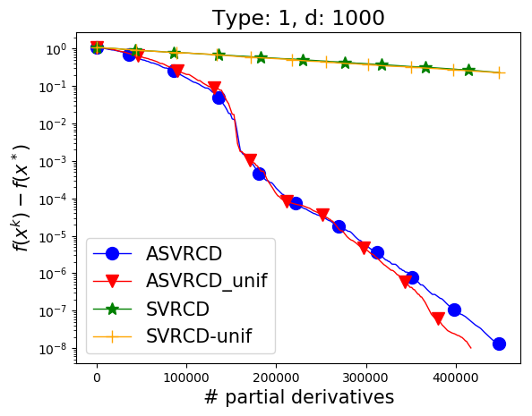
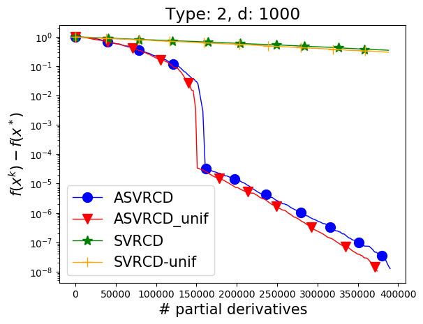
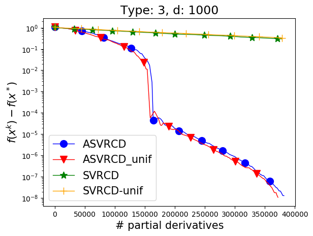
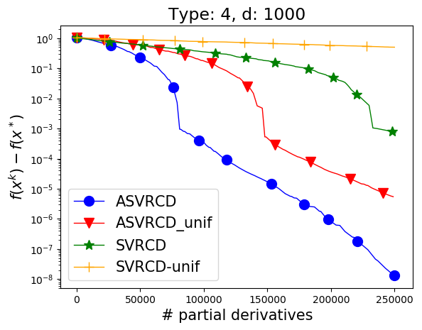
Figure 1: Comparison of both ASVRCD and SVRCD with importance and uniform sampling.

The second experiment compares the performance of both ASVRCD and SVRCD for various ${\bf W}$. We only consider methods with the importance sampling ($p_{i}\propto{\bf M}_{i,i}{\bf W}_{i,i}$) and theory supported stepsize. Figure 2 presents the result. We see that the smaller ${\rm Range}\left({\bf W}\right)$ is, the faster the convergence is. This observation is well-aligned with our theory: ${\cal L}$ is increasing as a function of ${\bf W}$ (in terms of Loewner ordering).

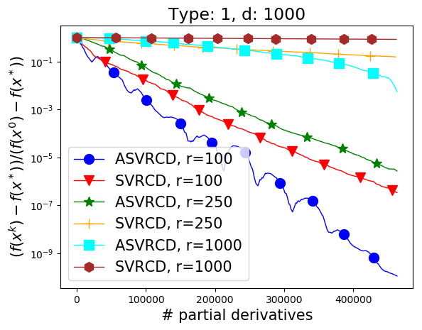
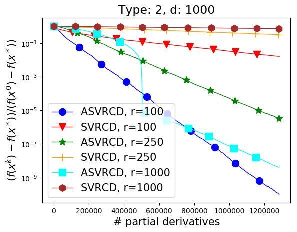
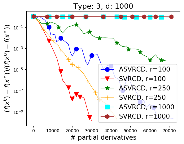
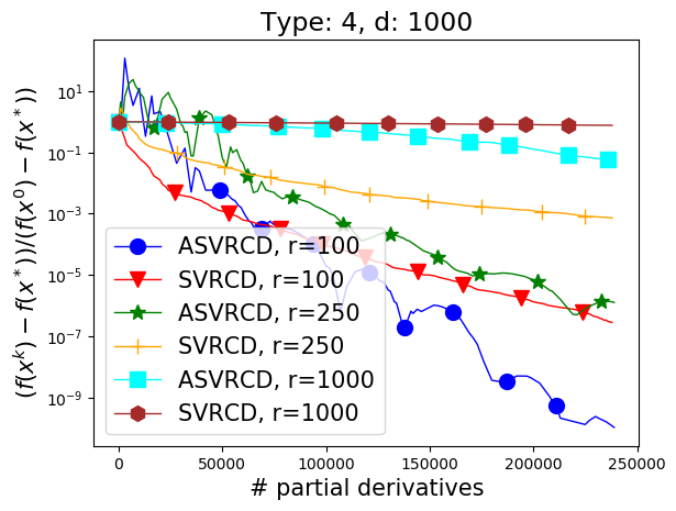
Figure 2: Comparison of ASVRCD and SVRCD for various ${\color[rgb]{0,0,0}}$. Label ’r’ indicates the dimension of ${\rm Range}\left({\color[rgb]{0,0,0}}\right)$.

7 Implications

Finite sum algorithms are a special case of methods with partial derivative oracle.

Using the trick described in Sections 3 and 5.2, it is possible to show that essentially any finite-sum stochastic algorithm is a special case of analogous method with partial derivative oracle (those are yet to be discovered/analyzed) in a given setting (i.e., strongly convex, convex, non-convex). Those include, but are not limited to SGD [32, 23], over-parametrized SGD [35], SAG [33], SVRG [16], S2GD [17], SARAH [27], incremental methods such as Finito [6], MISO [22] or accelerated algorithms such as point-SAGA [4], Katyusha [1], MiG [39], SAGA-SSNM [38], Catalyst [21, 20], non-convex variance reduced algorithms [30, 2, 7] and others. In particular, SGD can be seen as a special case of block coordinate descent, while SAG is a special case of bias-SEGA from [11] (neither of CD with non-separable prox, nor bias-SEGA were analyzed yet).

Zero order optimization with non-separable non-smooth regularizer.

We believe it would be interesting to develop an inexact version of ASVRCD, as this would immediately enable the application in zero-order optimization, where the partial derivatives are (inexactly) estimated using finite differences.

Acknowledgments

The authors would like to express their gratitude to Konstantin Mishchenko. In particular, Konstantin has introduced us to the product space objective (13) and at the same time, the idea that SAGA is a special case of SEGA was born during the discussion with him.

Appendix A SAGA and L-SVRG: The algorithm

Algorithm 4 SAGA/L-SVRG

0:  $\alpha>0$, ${\color[rgb]{0,0,0}\rho}\in(0,1)$

  ${\color[rgb]{1,0,0}x}^{0}\in\mathbb{R}^{\color[rgb]{1,0,0}d},{\bf J}^{0}=0\in\mathbb{R}^{d\times n}$

  for $k=0,1,2,\ldots$ do

     Sample random ${\color[rgb]{1,0,0}S}\subseteq\{1,\dots,n\}$

     ${\color[rgb]{1,0,0}g}^{k}=\frac{1}{n}{\bf J}^{k}{\color[rgb]{1,0,0}e}+\frac{1}{n}\sum\limits_{i\in{\color[rgb]{1,0,0}S}}\frac{1}{{{\color[rgb]{1,0,0}p}}_{i}}(\nabla{\color[rgb]{1,0,0}f}_{i}({\color[rgb]{1,0,0}x}^{k})-{\bf J}^{k}_{:,i})$

     ${\color[rgb]{1,0,0}x}^{k+1}=\mathop{\mathrm{prox}}\nolimits_{{\color[rgb]{1,0,0}\alpha}\psi}({\color[rgb]{1,0,0}x}^{k}-{\color[rgb]{1,0,0}\alpha}{\color[rgb]{1,0,0}g}^{k})$

     Update ${\bf J}^{k+1}$ according to (10) or (11)

  end for

Appendix B Missing lemmas and proofs: SAGA/L-SVRG is a special case of SEGA/SVRCD

B.1 Proof of Lemma 3.2

Let ${\color[rgb]{0,0,0}}^{\prime}\coloneqq\frac{1}{n}{\color[rgb]{1,0,0}e}{\color[rgb]{1,0,0}e}^{\top}\otimes{\bf I}$ and denote ${\bf D_{B}}({\color[rgb]{1,0,0}{\bf M}})\coloneqq\text{BlockDiag}({\color[rgb]{1,0,0}{\bf M}}_{1},\dots,{\color[rgb]{1,0,0}{\bf M}}_{n})$ for simplicity. Now clearly $x^{0}\in{\rm Range}\left({\color[rgb]{0,0,0}}^{\prime}\right)$, while ${\color[rgb]{0,0,0}}^{\prime}$ is a projection matrix such that $I(x)<\infty$ if and only if ${\color[rgb]{0,0,0}}^{\prime}x=x$. Consequently, ${\color[rgb]{0,0,0}}={\color[rgb]{0,0,0}}^{\prime}$. Next, if $x,y\in{\rm Range}\left({\color[rgb]{0,0,0}}\right)$, there is ${\color[rgb]{1,0,0}x},{\color[rgb]{1,0,0}y}\in\mathbb{R}^{\color[rgb]{1,0,0}d}$ such that $x=Q\left({\color[rgb]{1,0,0}x}\right),y=Q\left({\color[rgb]{1,0,0}y}\right)$. Therefore we can write

$$f(x)=f({\color[rgb]{0,0,0}}(x))=\frac{1}{n}\sum_{j=1}^{n}{\color[rgb]{1,0,0}f}_{j}({\color[rgb]{1,0,0}x}) \geq \frac{1}{n}\sum_{j=1}^{n}{\color[rgb]{1,0,0}f}_{j}({\color[rgb]{1,0,0}y})+\left\langle\nabla\left(\frac{1}{n}\sum_{j=1}^{n}{\color[rgb]{1,0,0}f}_{j}({\color[rgb]{1,0,0}y})\right),{\color[rgb]{1,0,0}x}-{\color[rgb]{1,0,0}y}\right\rangle+\frac{{\color[rgb]{1,0,0}\mu}}{2}\|{\color[rgb]{1,0,0}x}-{\color[rgb]{1,0,0}y}\|^{2}$$

$$= f(y)+\left\langle\nabla f(y),x-y\right\rangle+\frac{{\color[rgb]{1,0,0}\mu}}{2n}\|x-y\|^{2}.$$

Similarly,

$$f(x)=\frac{1}{n}\sum_{j=1}^{n}{\color[rgb]{1,0,0}f}_{j}({\color[rgb]{1,0,0}x}) \leq \frac{1}{n}\sum_{j=1}^{n}{\color[rgb]{1,0,0}f}_{j}({\color[rgb]{1,0,0}y})+\left\langle\nabla\left(\frac{1}{n}\sum_{j=1}^{n}{\color[rgb]{1,0,0}f}_{j}({\color[rgb]{1,0,0}y})\right),{\color[rgb]{1,0,0}x}-{\color[rgb]{1,0,0}y}\right\rangle+\sum_{j=1}^{n}\frac{1}{2n}\|{\color[rgb]{1,0,0}x}-{\color[rgb]{1,0,0}y}\|^{2}_{{\color[rgb]{1,0,0}{\bf M}}_{j}}$$

$$= f(y)+\left\langle\nabla f(y),x-y\right\rangle+\frac{1}{2n}\|x-y\|^{2}_{{\bf D_{B}}({\color[rgb]{1,0,0}{\bf M}})}.$$

Thus we conclude $\mu=\frac{{\color[rgb]{1,0,0}\mu}}{n}$ and ${\bf M}=\frac{1}{n}{\bf D_{B}}({\color[rgb]{1,0,0}{\bf M}})$. Further, for any $h\in\mathbb{R}^{d}$, we have:

$$h^{\top}{\bf M}^{\frac{1}{2}}\mathbb{E}\left[\sum_{i\in S}{\color[rgb]{0,0,0}p_{i}}^{-1}{\color[rgb]{0,0,0}e_{i}}{\color[rgb]{0,0,0}e_{i}}^{\top}{\color[rgb]{0,0,0}}\sum_{i\in S}{\color[rgb]{0,0,0}p_{i}}^{-1}{\color[rgb]{0,0,0}e_{i}}{\color[rgb]{0,0,0}e_{i}}^{\top}\right]{\bf M}^{\frac{1}{2}}{h}$$

$$\qquad=\frac{1}{n}h^{\top}{\bf D_{B}}({\color[rgb]{1,0,0}{\bf M}})^{\frac{1}{2}}\mathbb{E}\left[\left(\sum_{i\in{\color[rgb]{1,0,0}S}}{\color[rgb]{1,0,0}p}_{i}^{-1}\left(\sum_{j\in R_{i}}e_{j}e_{j}^{\top}\right)\right){\color[rgb]{0,0,0}}\left(\sum_{i\in{\color[rgb]{1,0,0}S}}{\color[rgb]{1,0,0}p}_{i}^{-1}\left(\sum_{j\in R_{i}}e_{j}e_{j}^{\top}\right)\right)\right]{\bf D_{B}}({\color[rgb]{1,0,0}{\bf M}})^{\frac{1}{2}}{h}$$

$$\qquad=\frac{1}{n}\mathbb{E}\left[\left\|\sum_{i\in{\color[rgb]{1,0,0}S}}{\color[rgb]{1,0,0}{\bf M}}^{\frac{1}{2}}_{i}{\color[rgb]{1,0,0}p}_{i}^{-1}h_{R_{i}}\right\|^{2}\right]$$

$$\qquad\stackrel{{\scriptstyle\eqref{eq:ESO_saga}}}{{\leq}}\frac{1}{n}\sum_{i=1}^{n}{\color[rgb]{1,0,0}p}_{i}{\color[rgb]{1,0,0}v}_{i}\left\|h_{R_{i}}\right\|^{2}$$

and thus (6) holds with $v=\frac{1}{n}{\color[rgb]{1,0,0}v}$ as desired.

B.2 Proof of Lemma 3.3

Denote $\mbox{Vec}\left(\cdot\right)$ to be the vectorization operator, i.e., operator which takes a matrix as an input, and returns a vector constructed by a column-wise stacking of the matrix columns. We will show both

$$h^{k}=\frac{1}{n}\mbox{Vec}\left({\bf J}^{k}\right)$$ (19)

and (14) using mathematical induction. Clearly, if $k=0$ both (19) and (14) hold. Now, let us proceed with the second induction step.

$$x^{k+1} = \mathop{\mathrm{prox}}\nolimits_{\alpha\psi}(x^{k}-\alpha g^{k})=\operatorname*{argmin}_{x\in\mathbb{R}^{d}}\,\alpha I(x)+\alpha{\color[rgb]{1,0,0}\psi}(x_{R_{1}})+\|x-(x^{k}-\alpha g^{k})\|^{2}$$ (20)

$$= \operatorname*{argmin}_{x\in\mathbb{R}^{d}}\,\alpha I(x)+\alpha{\color[rgb]{1,0,0}\psi}(x_{R_{1}})+\left\|x-x^{k}+\alpha\left(h^{k}+\sum\limits_{i\in S}\frac{1}{{\color[rgb]{0,0,0}p_{i}}}(\nabla_{i}f(x^{k})-h_{i}^{k}){\color[rgb]{0,0,0}e_{i}}\right)\right\|^{2}$$

$$= \operatorname*{argmin}_{x={\color[rgb]{0,0,0}}x}\,\alpha{\color[rgb]{1,0,0}\psi}(x_{R_{1}})+\left\|x-x^{k}+\alpha\left(h^{k}+\sum\limits_{i\in S}\frac{1}{{\color[rgb]{0,0,0}p_{i}}}(\nabla_{i}f(x^{k})-h_{i}^{k}){\color[rgb]{0,0,0}e_{i}}\right)\right\|^{2}$$

$$= \operatorname*{argmin}_{x={\color[rgb]{0,0,0}}x}\,\alpha{\color[rgb]{1,0,0}\psi}(x_{R_{1}})+\left\|x-x^{k}+\alpha\left(h^{k}+\sum\limits_{i\in S}\frac{1}{{\color[rgb]{0,0,0}p_{i}}}(\nabla_{i}f(x^{k})-h_{i}^{k}){\color[rgb]{0,0,0}e_{i}}\right)\right\|^{2}_{{\color[rgb]{0,0,0}}}$$

$$\stackrel{{\scriptstyle\eqref{eq:iterates_equivalence}}}{{=}} Q\left(\operatorname*{argmin}_{{\color[rgb]{1,0,0}x}\in\mathbb{R}^{\color[rgb]{1,0,0}d}}\,\alpha{\color[rgb]{1,0,0}\psi}({\color[rgb]{1,0,0}x})+\left\|Q\left({\color[rgb]{1,0,0}x}\right)-Q\left({\color[rgb]{1,0,0}x}^{k}\right)+\alpha\left(h^{k}+\sum\limits_{i\in{\color[rgb]{1,0,0}S}}\frac{1}{{\color[rgb]{1,0,0}p}_{i}}\left(\sum_{j\in R_{i}}\left(\frac{1}{n}\nabla_{j}{\color[rgb]{1,0,0}f}_{i}({\color[rgb]{1,0,0}x}^{k})-h_{(i-1){\color[rgb]{1,0,0}d}+j}^{k}\right)e_{(i-1){\color[rgb]{1,0,0}d}+j}\right)\right)\right\|^{2}_{{\color[rgb]{0,0,0}}}\right)$$

$$= Q\left(\operatorname*{argmin}_{{\color[rgb]{1,0,0}x}\in\mathbb{R}^{\color[rgb]{1,0,0}d}}\,\alpha{\color[rgb]{1,0,0}\psi}({\color[rgb]{1,0,0}x})+\frac{1}{n}\left\|n{\color[rgb]{1,0,0}x}-n{\color[rgb]{1,0,0}x}^{k}+\alpha\left(\sum_{i=1}^{n}h^{k}_{R_{i}}+\sum\limits_{i\in{\color[rgb]{1,0,0}S}}\frac{1}{{\color[rgb]{1,0,0}p}_{i}}\left(\frac{1}{n}\nabla{\color[rgb]{1,0,0}f}_{i}({\color[rgb]{1,0,0}x}^{k})-h_{R_{i}}^{k}\right)\right)\right\|^{2}\right)$$

$$\stackrel{{\scriptstyle\eqref{eq:hj_equivalence}}}{{=}} Q\left(\operatorname*{argmin}_{{\color[rgb]{1,0,0}x}\in\mathbb{R}^{\color[rgb]{1,0,0}d}}\,\alpha{\color[rgb]{1,0,0}\psi}({\color[rgb]{1,0,0}x})+\frac{1}{n}\left\|n{\color[rgb]{1,0,0}x}-n{\color[rgb]{1,0,0}x}^{k}+\alpha\left(\frac{1}{n}{\bf J}^{k}{\color[rgb]{1,0,0}e}+\frac{1}{n}\sum\limits_{i\in{\color[rgb]{1,0,0}S}}\frac{1}{{\color[rgb]{1,0,0}p}_{i}}\left((\nabla{\color[rgb]{1,0,0}f}_{i}({\color[rgb]{1,0,0}x}^{k})-{\bf J}^{k}_{:,i})\right)\right)\right\|^{2}\right)$$

$$= Q\left(\operatorname*{argmin}_{{\color[rgb]{1,0,0}x}\in\mathbb{R}^{\color[rgb]{1,0,0}d}}\,{\color[rgb]{1,0,0}\alpha}{\color[rgb]{1,0,0}\psi}({\color[rgb]{1,0,0}x})+\left\|{\color[rgb]{1,0,0}x}-{\color[rgb]{1,0,0}x}^{k}+{\color[rgb]{1,0,0}\alpha}\left(\frac{1}{n}{\bf J}^{k}{\color[rgb]{1,0,0}e}+\frac{1}{n}\sum\limits_{i\in{\color[rgb]{1,0,0}S}}\frac{1}{{\color[rgb]{1,0,0}p}_{i}}\left((\nabla{\color[rgb]{1,0,0}f}_{i}({\color[rgb]{1,0,0}x}^{k})-{\bf J}^{k}_{:,i})\right)\right)\right\|^{2}\right)$$

$$= Q\left({\color[rgb]{1,0,0}x}^{k+1}\right).$$

It remains to notice that since $x^{k+1}=Q\left({\color[rgb]{1,0,0}x}^{k}\right)$, we have $h^{k+1}=\frac{1}{n}\mbox{Vec}\left({\bf J}^{k+1}\right)$ as desired.

Appendix C Missing lemmas and proofs: ASVRCD

C.1 Technical lemmas

We first start with two key technical lemmas.

Lemma C.1

Suppose that

$$\eta\leq\frac{1}{2L}.$$ (21)

Then, for all $x\in{\rm Range}\left({\color[rgb]{0,0,0}}\right)$ the following inequality holds:

$$\frac{1}{\eta}\mathbb{E}\left[\left\langle x-x^{k},x^{k}-y^{k+1}\right\rangle\right] \leq\mathbb{E}\left[P(x)-P(y^{k+1})-\frac{1}{4\eta}\left\|y^{k+1}-x^{k}\right\|^{2}+\frac{\eta}{2}\left\|g^{k}-\nabla f(x^{k})\right\|^{2}_{\color[rgb]{0,0,0}}\right]-D_{f}(x,x^{k}).$$ (22)

Proof: From the definition of $y^{k+1}$ we get

$$y^{k+1}=x^{k}-\eta g^{k}-\eta\Delta,$$

where $\Delta\in\partial\psi(y^{k+1})$. Therefore,

$$\mathbb{E}\left[\frac{1}{\eta}\left\langle x-x^{k},x^{k}-y^{k+1}\right\rangle\right] =\mathbb{E}\left[\left\langle x-x^{k},g^{k}+\Delta\right\rangle\right]$$

$$=\left\langle x-x^{k},\nabla f(x^{k})\right\rangle+\mathbb{E}\left[\left\langle x-y^{k+1},\Delta\right\rangle+\left\langle y^{k+1}-x^{k},\Delta\right\rangle\right]$$

$$\leq f(x)-f(x^{k})-D_{f}(x,x^{k})+\mathbb{E}\left[\psi(x)-\psi(y^{k+1})\right]+\mathbb{E}\left[\left\langle y^{k+1}-x^{k},\Delta\right\rangle\right]$$ (23)

Now, we use the fact that $f$ is $L$-smooth over the set where iterates live (i.e., over $\{x^{0}+{\rm Range}\left({\color[rgb]{0,0,0}}\right)\}$):

$$f(y^{k+1}) \leq f(x^{k})+\left\langle\nabla f(x^{k}),y^{k+1}-x^{k}\right\rangle+\frac{L}{2}\left\|y^{k+1}-x^{k}\right\|^{2}$$ (24)

$$= f(x^{k})+\left\langle{\color[rgb]{0,0,0}}\nabla f(x^{k}),y^{k+1}-x^{k}\right\rangle+\frac{L}{2}\left\|y^{k+1}-x^{k}\right\|^{2}.$$

Thus, we have

$$\mathbb{E}\left[\frac{1}{\eta}\left\langle x-x^{k},x^{k}-y^{k+1}\right\rangle\right]$$

$$\,\,\,\,\,\stackrel{{\scriptstyle\eqref{eq:dnjansdjkajksd}+\eqref{eq:dabhusdbhu}}}{{\leq}}\mathbb{E}\left[P(x)-P(y^{k+1})+\left\langle y^{k+1}-x^{k},{\color[rgb]{0,0,0}}(\Delta+\nabla f(x^{k}))\right\rangle+\frac{L}{2}\left\|y^{k+1}-x^{k}\right\|^{2}\right]$$

$$\qquad\qquad-D_{f}(x,x^{k})$$

$$\qquad=\mathbb{E}\left[P(x)-P(y^{k+1})+\left\langle y^{k+1}-x^{k},{\color[rgb]{0,0,0}}(\nabla f(x^{k})-g^{k})\right\rangle-\frac{1}{\eta}\left\|y^{k+1}-x^{k}\right\|^{2}\right]$$

$$\qquad\qquad+\mathbb{E}\left[\frac{L}{2}\left\|y^{k+1}-x^{k}\right\|^{2}\right]-D_{f}(x,x^{k})$$

$$\qquad\leq\mathbb{E}\left[P(x)-P(y^{k+1})+\frac{\eta}{2}\left\|\nabla f(x^{k})-g^{k}\right\|^{2}_{\color[rgb]{0,0,0}}-\frac{1}{2\eta}\left\|y^{k+1}-x^{k}\right\|^{2}+\frac{L}{2}\left\|y^{k+1}-x^{k}\right\|\right]$$

$$\qquad\qquad-D_{f}(x,x^{k})$$

$$\qquad\stackrel{{\scriptstyle\eqref{eq:mkdkmd}}}{{\leq}}\mathbb{E}\left[P(x)-P(y^{k+1})-\frac{1}{4\eta}\left\|y^{k+1}-x^{k}\right\|^{2}+\frac{\eta}{2}\left\|\nabla f(x^{k})-g^{k}\right\|^{2}_{\color[rgb]{0,0,0}}\right]-D_{f}(x,x^{k}),$$

which concludes the proof.

Lemma C.2

Suppose, the following choice of parameters is used:

$$\eta=\frac{1}{4}\max\{{\color[rgb]{0,0,1}{\cal L}^{\prime}},L\}^{-1},\qquad\gamma=\frac{1}{\max\{2\mu,4\theta_{1}/\eta\}},\qquad\beta=1-\gamma\mu,\qquad\theta_{2}=\frac{{\color[rgb]{0,0,1}{\cal L}^{\prime}}}{2\max\{L,{\color[rgb]{0,0,1}{\cal L}^{\prime}}\}}.$$

Then the following inequality holds:

$$\mathbb{E}\left[\left\|z^{k+1}-x^{*}\right\|^{2}+\frac{2\gamma\beta}{\theta_{1}}\left[P(y^{k+1})-P(x^{*})\right]\right]$$

$$\qquad\leq\beta\left\|z^{k}-x^{*}\right\|^{2}+\frac{2\gamma\beta\theta_{2}}{\theta_{1}}\left[P(w^{k})-P(x^{*})\right]+\frac{2\gamma\beta(1-\theta_{1}-\theta_{2})}{\theta_{1}}\left[P(y^{k})-P(x^{*})\right].$$ (25)

Proof:

$$\mathbb{E}\left[\left\|z^{k+1}-x^{*}\right\|^{2}\right] =\mathbb{E}\left[\left\|\beta z^{k}+(1-\beta)x^{k}-x^{*}+\frac{\gamma}{\eta}(y^{k+1}-x^{k})\right\|^{2}\right]$$

$$\leq\beta\left\|z^{k}-x^{*}\right\|^{2}+(1-\beta)\left\|x^{k}-x^{*}\right\|^{2}+\frac{\gamma^{2}}{\eta^{2}}\mathbb{E}\left[\left\|y^{k+1}-x^{k}\right\|^{2}\right]$$

$$\qquad+\frac{2\gamma}{\eta}\mathbb{E}\left[\left\langle y^{k+1}-x^{k},\beta z^{k}+(1-\beta)x^{k}-x^{*}\right\rangle\right]$$

$$=\beta\left\|z^{k}-x^{*}\right\|^{2}+(1-\beta)\left\|x^{k}-x^{*}\right\|^{2}+\frac{\gamma^{2}}{\eta^{2}}\mathbb{E}\left[\left\|y^{k+1}-x^{k}\right\|^{2}\right]$$

$$\qquad+\frac{2\gamma}{\eta}\mathbb{E}\left[\left\langle y^{k+1}-x^{k},x^{k}-x^{*}\right\rangle\right]+\frac{2\gamma\beta}{\eta}\mathbb{E}\left[\left\langle y^{k+1}-x^{k},z^{k}-x^{k}\right\rangle\right]$$

$$=\beta\left\|z^{k}-x^{*}\right\|^{2}+(1-\beta)\left\|x^{k}-x^{*}\right\|^{2}+\frac{\gamma^{2}}{\eta^{2}}\mathbb{E}\left[\left\|y^{k+1}-x^{k}\right\|^{2}\right]+\frac{2\gamma}{\eta}\mathbb{E}\left[\left\langle x^{k}-y^{k+1},x^{*}-x^{k}\right\rangle\right]$$

$$\qquad+\frac{2\gamma\beta\theta_{2}}{\eta\theta_{1}}\mathbb{E}\left[\left\langle x^{k}-y^{k+1},w^{k}-x^{k}\right\rangle\right]+\frac{2\gamma\beta(1-\theta_{1}-\theta_{2})}{\eta\theta_{1}}\mathbb{E}\left[\left\langle x^{k}-y^{k+1},y^{k}-x^{k}\right\rangle\right]$$

$$\stackrel{{\scriptstyle\eqref{eq:keylemma_acc}}}{{\leq}}\beta\left\|z^{k}-x^{*}\right\|^{2}+(1-\beta)\left\|x^{k}-x^{*}\right\|^{2}+\frac{\gamma^{2}}{\eta^{2}}\mathbb{E}\left[\left\|y^{k+1}-x^{k}\right\|^{2}\right]$$

$$\qquad+2\gamma\mathbb{E}\left[P(x^{*})-P(y^{k+1})-\frac{1}{4\eta}\left\|y^{k+1}-x^{k}\right\|^{2}-D_{f}(x^{*},x^{k})+\frac{\eta}{2}\left\|g^{k}-\nabla f(x^{k})\right\|^{2}_{\color[rgb]{0,0,0}}\right]$$

$$\qquad+\frac{2\gamma\beta\theta_{2}}{\theta_{1}}\mathbb{E}\left[P(w^{k})-P(y^{k+1})-\frac{1}{4\eta}\left\|y^{k+1}-x^{k}\right\|^{2}-D_{f}(w^{k},x^{k})+\frac{\eta}{2}\left\|g^{k}-\nabla f(x^{k})\right\|^{2}_{\color[rgb]{0,0,0}}\right]$$

$$\qquad+\frac{2\gamma\beta(1-\theta_{1}-\theta_{2})}{\theta_{1}}\mathbb{E}\left[P(y^{k})-P(y^{k+1})-\frac{1}{4\eta}\left\|y^{k+1}-x^{k}\right\|^{2}+\frac{\eta}{2}\left\|g^{k}-\nabla f(x^{k})\right\|^{2}_{\color[rgb]{0,0,0}}\right]$$

$$\stackrel{{\scriptstyle\eqref{eq:sc}}}{{\leq}}\beta\left\|z^{k}-x^{*}\right\|^{2}+(1-\beta-\gamma\mu)\left\|x^{k}-x^{*}\right\|^{2}+\frac{\gamma^{2}}{\eta^{2}}\mathbb{E}\left[\left\|y^{k+1}-x^{k}\right\|^{2}\right]$$

$$\qquad+2\gamma\beta\mathbb{E}\left[P(x^{*})-P(y^{k+1})-\frac{1}{4\eta}\left\|y^{k+1}-x^{k}\right\|^{2}\right]+\eta\gamma\mathbb{E}\left[\left\|g^{k}-\nabla f(x^{k})\right\|^{2}_{\color[rgb]{0,0,0}}\right]$$

$$\qquad+\frac{2\gamma\beta\theta_{2}}{\theta_{1}}\mathbb{E}\left[P(w^{k})-P(y^{k+1})-\frac{1}{4\eta}\left\|y^{k+1}-x^{k}\right\|^{2}-D_{f}(w^{k},x^{k})+\frac{\eta}{2}\left\|g^{k}-\nabla f(x^{k})\right\|^{2}_{\color[rgb]{0,0,0}}\right]$$

$$\qquad+\frac{2\gamma\beta(1-\theta_{1}-\theta_{2})}{\theta_{1}}\mathbb{E}\left[P(y^{k})-P(y^{k+1})-\frac{1}{4\eta}\left\|y^{k+1}-x^{k}\right\|^{2}+\frac{\eta}{2}\left\|g^{k}-\nabla f(x^{k})\right\|^{2}_{\color[rgb]{0,0,0}}\right].$$

Using $\beta=1-\gamma\mu$ we get

$$\mathbb{E}\left[\left\|z^{k+1}-x^{*}\right\|^{2}\right] \leq\beta\left\|z^{k}-x^{*}\right\|^{2}+\left[\frac{\gamma^{2}}{\eta^{2}}-\frac{\gamma\beta}{2\eta\theta_{1}}\right]\mathbb{E}\left[\left\|y^{k+1}-x^{k}\right\|^{2}\right]+\frac{\eta\gamma}{\theta_{1}}\mathbb{E}\left[\left\|g^{k}-\nabla f(x^{k})\right\|^{2}_{\color[rgb]{0,0,0}}\right]$$

$$\qquad-\frac{2\gamma\beta\theta_{2}}{\theta_{1}}D_{f}(w^{k},x^{k})+2\gamma\beta\mathbb{E}\left[P(x^{*})-P(y^{k+1})\right]$$

$$\qquad+\frac{2\gamma\beta\theta_{2}}{\theta_{1}}\mathbb{E}\left[P(w^{k})-P(y^{k+1})\right]+\frac{2\gamma\beta(1-\theta_{1}-\theta_{2})}{\theta_{1}}\mathbb{E}\left[P(y^{k})-P(y^{k+1})\right].$$

Using stepsize $\gamma\leq\frac{\beta\eta}{2\theta_{1}}$ we get

$$\mathbb{E}\left[\left\|z^{k+1}-x^{*}\right\|^{2}\right] \leq\beta\left\|z^{k}-x^{*}\right\|^{2}+\frac{\eta\gamma}{\theta_{1}}\mathbb{E}\left[\left\|g^{k}-\nabla f(x^{k})\right\|^{2}_{\color[rgb]{0,0,0}}\right]-\frac{2\gamma\beta\theta_{2}}{\theta_{1}}D_{f}(w^{k},x^{k})+2\gamma\beta\mathbb{E}\left[P(x^{*})-P(y^{k+1})\right]$$

$$\qquad+\frac{2\gamma\beta\theta_{2}}{\theta_{1}}\mathbb{E}\left[P(w^{k})-P(y^{k+1})\right]+\frac{2\gamma\beta(1-\theta_{1}-\theta_{2})}{\theta_{1}}\mathbb{E}\left[P(y^{k})-P(y^{k+1})\right].$$

Now, using the expected smoothness from inequality (16):

$$\mathbb{E}\left[\left\|g^{k}-\nabla f(x^{k})\right\|^{2}_{\color[rgb]{0,0,0}}\right]\leq 2{\color[rgb]{0,0,1}{\cal L}^{\prime}}D_{f}(w^{k},x^{k})$$ (26)

and stepsize $\eta\leq\frac{\beta\theta_{2}}{{\color[rgb]{0,0,1}{\cal L}^{\prime}}}$ we get

$$\mathbb{E}\left[\left\|z^{k+1}-x^{*}\right\|^{2}\right] \leq\beta\left\|z^{k}-x^{*}\right\|^{2}+\frac{2{\color[rgb]{0,0,1}{\cal L}^{\prime}}\eta\gamma}{\theta_{1}}D_{f}(w^{k},x^{k})-\frac{2\gamma\beta\theta_{2}}{\theta_{1}}D_{f}(w^{k},x^{k})+2\gamma\beta\mathbb{E}\left[P(x^{*})-P(y^{k+1})\right]$$

$$\qquad+\frac{2\gamma\beta\theta_{2}}{\theta_{1}}\mathbb{E}\left[P(w^{k})-P(y^{k+1})\right]+\frac{2\gamma\beta(1-\theta_{1}-\theta_{2})}{\theta_{1}}\mathbb{E}\left[P(y^{k})-P(y^{k+1})\right]$$

$$\leq\beta\left\|z^{k}-x^{*}\right\|^{2}+2\gamma\beta\mathbb{E}\left[P(x^{*})-P(y^{k+1})\right]+\frac{2\gamma\beta\theta_{2}}{\theta_{1}}\mathbb{E}\left[P(w^{k})-P(y^{k+1})\right]$$

$$\qquad+\frac{2\gamma\beta(1-\theta_{1}-\theta_{2})}{\theta_{1}}\mathbb{E}\left[P(y^{k})-P(y^{k+1})\right]$$

$$=\beta\left\|z^{k}-x^{*}\right\|^{2}-\frac{2\gamma\beta}{\theta_{1}}\mathbb{E}\left[P(y^{k+1})-P(x^{*})\right]+\frac{2\gamma\beta\theta_{2}}{\theta_{1}}\left[P(w^{k})-P(x^{*})\right]$$

$$\qquad+\frac{2\gamma\beta(1-\theta_{1}-\theta_{2})}{\theta_{1}}\left[P(y^{k})-P(x^{*})\right].$$

It remains to rearrange the terms.

C.2 Proof of Theorem 4.1

One can easily show that

$$\mathbb{E}\left[P(w^{k+1})\right]={\color[rgb]{0,0,0}\rho}P(y^{k})+(1-{\color[rgb]{0,0,0}\rho})P(w^{k}).$$ (27)

Using that we obtain

$$\mathbb{E}\left[\Psi^{k+1}\right] \stackrel{{\scriptstyle\eqref{eq:nhivbhi}+\eqref{eq:bfrbuf}}}{{\leq}} \beta\left\|z^{k}-x^{*}\right\|^{2}+\frac{2\gamma\beta\theta_{2}}{\theta_{1}}\left[P(w^{k})-P(x^{*})\right]+\frac{2\gamma\beta(1-\theta_{1}-\theta_{2})}{\theta_{1}}\left[P(y^{k})-P(x^{*})\right]$$

$$\qquad+\frac{(2\theta_{2}+\theta_{1})\gamma\beta}{\theta_{1}{\color[rgb]{0,0,0}\rho}}\left[{\color[rgb]{0,0,0}\rho}P(y^{k})+(1-{\color[rgb]{0,0,0}\rho})P(w^{k})-P(x^{*})\right]$$

$$= \beta\left\|z^{k}-x^{*}\right\|^{2}+\frac{2\gamma\beta(1-\theta_{1}/2)}{\theta_{1}}\left[P(y^{k})-P(x^{*})\right]$$

$$\qquad+\frac{(2\theta_{2}+\theta_{1})\gamma\beta}{\theta_{1}{\color[rgb]{0,0,0}\rho}}\left[1-{\color[rgb]{0,0,0}\rho}+\frac{2{\color[rgb]{0,0,0}\rho}\theta_{2}}{2\theta_{2}+\theta_{1}}\right]\left[P(w^{k})-P(x^{*})\right]$$

$$\leq \max\left\{1-\frac{1}{\max\{2,4\theta_{1}/(\eta\mu)\}},1-\frac{\theta_{1}}{2},1-\frac{{\color[rgb]{0,0,0}\rho}\theta_{1}}{2\max\{2\theta_{2},\theta_{1}\}}\right\}\Psi^{k}$$

$$= \left[1-\max\left\{\frac{2}{{\color[rgb]{0,0,0}\rho}},\frac{4}{\theta_{1}}\max\left\{\frac{1}{2},\frac{\theta_{2}}{\rho}\right\},\frac{4\theta_{1}}{\eta\mu}\right\}^{-1}\right]\Psi^{k}.$$

Using $\theta_{1}=\min\left\{\frac{1}{2},\sqrt{\eta\mu\max\left\{\frac{1}{2},\frac{\theta_{2}}{\rho}\right\}}\right\}$ we get

$$\mathbb{E}\left[\Psi^{k+1}\right] \leq\left[1-\max\left\{\frac{2}{{\color[rgb]{0,0,0}\rho}},8\max\left\{\frac{1}{2},\frac{\theta_{2}}{\rho}\right\},4\sqrt{\frac{\max\left\{\frac{1}{2},\frac{\theta_{2}}{\rho}\right\}}{\eta\mu}}\right\}^{-1}\right]\Psi^{k}$$

$$\leq\left[1-\frac{1}{4}\max\left\{\frac{1}{{\color[rgb]{0,0,0}\rho}},\sqrt{\frac{2\max\left\{L,\frac{{\color[rgb]{0,0,1}{\cal L}^{\prime}}}{\rho}\right\}}{\mu}}\right\}^{-1}\right]\Psi^{k},$$

as desired.

C.3 Proof of Lemma 4.2

To establish that that we can choose ${\color[rgb]{0,0,1}{\cal L}^{\prime}}={\cal L}$, it suffices to see

$$\mathbb{E}\left[\left\|g^{k}-\nabla f(x^{k})\right\|^{2}_{\color[rgb]{0,0,0}}\right] = \mathbb{E}\left[\left\|\sum\limits_{i\in S}\frac{1}{{\color[rgb]{0,0,0}p_{i}}}(\nabla_{i}f(x^{k})-\nabla_{i}f(w^{k}))e_{i}+\nabla f(w^{k})-\nabla f(x^{k})\right\|^{2}_{\color[rgb]{0,0,0}}\right]$$

$$\leq \mathbb{E}\left[\left\|\sum\limits_{i\in S}\frac{1}{{\color[rgb]{0,0,0}p_{i}}}(\nabla_{i}f(x^{k})-\nabla_{i}f(w^{k}))e_{i}\right\|^{2}_{\color[rgb]{0,0,0}}\right]$$

$$\stackrel{{\scriptstyle\eqref{eq:ccLdef}}}{{\leq}} {\cal L}\left\|\nabla f(x^{k})-\nabla f(w^{k})\right\|^{2}_{{\bf M}^{-1}}$$

$$\stackrel{{\scriptstyle\eqref{eq:smooth}}}{{\leq}} 2{\cal L}D_{f}(w^{k},x^{k}).$$

Next, to establish ${\cal L}\geq L$, let ${\bf Q}\coloneqq\sum_{i\in S}\frac{1}{{\color[rgb]{0,0,0}p_{i}}}{\color[rgb]{0,0,0}e_{i}}{\color[rgb]{0,0,0}e_{i}}^{\top}{\color[rgb]{0,0,0}}$. Consequently, we get

$${\cal L} \stackrel{{\scriptstyle\eqref{eq:ccLdef}}}{{=}} \lambda_{\max}\left({\bf M}^{\frac{1}{2}}\mathbb{E}\left[\sum_{i\in S}\frac{1}{{\color[rgb]{0,0,0}p_{i}}}{\color[rgb]{0,0,0}e_{i}}{\color[rgb]{0,0,0}e_{i}}^{\top}{\color[rgb]{0,0,0}}\sum_{i\in S}\frac{1}{{\color[rgb]{0,0,0}p_{i}}}{\color[rgb]{0,0,0}e_{i}}{\color[rgb]{0,0,0}e_{i}}^{\top}\right]{\bf M}^{\frac{1}{2}}\right)$$

$$= \lambda_{\max}\left({\bf M}^{\frac{1}{2}}\mathbb{E}\left[\sum_{i\in S}\frac{1}{{\color[rgb]{0,0,0}p_{i}}}{\color[rgb]{0,0,0}e_{i}}{\color[rgb]{0,0,0}e_{i}}^{\top}{\color[rgb]{0,0,0}}^{2}\sum_{i\in S}\frac{1}{{\color[rgb]{0,0,0}p_{i}}}{\color[rgb]{0,0,0}e_{i}}{\color[rgb]{0,0,0}e_{i}}^{\top}\right]{\bf M}^{\frac{1}{2}}\right)$$

$$= \lambda_{\max}\left({\bf M}^{\frac{1}{2}}\mathbb{E}\left[{\bf Q}{\bf Q}^{\top}\right]{\bf M}^{\frac{1}{2}}\right)$$

$$\geq \lambda_{\max}\left({\bf M}^{\frac{1}{2}}\mathbb{E}\left[{\bf Q}\right]\mathbb{E}\left[{\bf Q}^{\top}\right]{\bf M}^{\frac{1}{2}}\right)$$

$$= \lambda_{\max}\left({\bf M}^{\frac{1}{2}}{\color[rgb]{0,0,0}}^{2}{\bf M}^{\frac{1}{2}}\right)$$

$$= \lambda_{\max}\left({\bf M}^{\frac{1}{2}}{\color[rgb]{0,0,0}}{\bf M}^{\frac{1}{2}}\right)$$

$$= L,$$

as desired.

C.4 Proof of Lemma 4.3

Let us look first at ${\color[rgb]{0,0,0}}={\bf I}$. In such case, it is easy to see that

$$\mathbb{E}\left[\left\|g^{k}-\nabla f(x^{k})\right\|^{2}_{{\color[rgb]{0,0,0}}}\right] =\mathbb{E}\left[\left\|g^{k}-\nabla f(x^{k})\right\|^{2}\right]$$

$$\leq\mathbb{E}\left[\left\|d(\nabla_{i}f(x^{k})-\nabla_{i}f(w^{k}))e_{i}\right\|^{2}\right]$$

$$=d\left\|\nabla f(x^{k})-\nabla f(w^{k})\right\|^{2}$$

$$\leq 2d\lambda_{\max}{\bf M}D_{f}(w^{k},x^{k}),$$

i. e. we can choose ${\color[rgb]{0,0,1}{\cal L}^{\prime}}=d\lambda_{\max}{\bf M}$. Noting that $\lambda_{\max}{\bf M}\geq L$, the iteration complexity of Algorithm 2 is ${\cal O}\left(d\sqrt{\frac{L}{\mu}}\log\frac{1}{\epsilon}\right)$.

On the other hand, if ${\color[rgb]{0,0,0}}=\frac{1}{d}{\color[rgb]{1,0,0}e}^{\top}$, we have

$$\mathbb{E}\left[\left\|g^{k}-\nabla f(x^{k})\right\|^{2}_{{\color[rgb]{0,0,0}}}\right]= \mathbb{E}\left[\left\|g^{k}-\nabla f(x^{k})\right\|^{2}_{\frac{1}{d}ee^{\top}}\right]$$

$$\leq\mathbb{E}\left[\left\|d(\nabla_{i}f(x^{k})-\nabla_{i}f(w^{k}))e_{i}\right\|^{2}_{\frac{1}{d}ee^{\top}}\right]$$

$$=\left\|\nabla f(x^{k})-\nabla f(w^{k})\right\|^{2}$$

$$\leq 2\lambda_{\max}{\bf M}D_{f}(w^{k},x^{k}),$$

and therefore ${\color[rgb]{0,0,1}{\cal L}^{\prime}}=\lambda_{\max}{\bf M}$, which yields ${\cal O}\left(\sqrt{\frac{d\lambda_{\max}{\bf M}}{\mu}}\log\frac{1}{\epsilon}\right)$ convergence rate.

Appendix D Missing lemmas and proofs: L-Katyusha as a particular case of ASVRCD

D.1 Proof of Lemma 5.2

Let us proceed by induction. We will show the following for all $k\geq 0$ we have

$${\color[rgb]{1,0,0}x}^{k}=x^{k}_{R_{1}}=\dots=x^{k}_{R_{n}},\;{\color[rgb]{1,0,0}y}^{k}=y^{k}_{R_{1}}=\dots=y^{k}_{R_{n}},\;{\color[rgb]{1,0,0}z}^{k}=z^{k}_{R_{1}}=\dots=z^{k}_{R_{n}}\;\mathrm{and}\>{\color[rgb]{1,0,0}w}^{k}=w^{k}_{R_{1}}=\dots=w^{k}_{R_{n}}.$$ (28)

Clearly, for $k=0$, the above claim holds. Let us proceed with the second induction step and assume that (28) holds for some $k\geq 0$. First, the update rule on $\{x^{k}\}$ for ASVRCD together with the update rule on $\{{\color[rgb]{1,0,0}x}^{k}\}$ yields

$${\color[rgb]{1,0,0}x}^{k+1}=x^{k+1}_{R_{1}}=\dots=x^{k+1}_{R_{n}}.$$ (29)

To show

$${\color[rgb]{1,0,0}y}^{k+1}=y^{k+1}_{R_{1}}=\dots=y^{k+1}_{R_{n}},$$ (30)

we essentially repeat the proof of Lemma 3.3. In particular, it is sufficient to repeat the sequence of inequalities (20) where variables

$$(x^{k+1},{\color[rgb]{1,0,0}x}^{k+1},h^{k},{\bf J}^{k}\alpha,{\color[rgb]{1,0,0}\alpha})$$

are replaced by

$$(y^{k+1},{\color[rgb]{1,0,0}y}^{k+1},\nabla f(w^{k}),[\nabla{\color[rgb]{1,0,0}f}_{1}({\color[rgb]{1,0,0}w}^{k}),\dots,\nabla{\color[rgb]{1,0,0}f}_{n}({\color[rgb]{1,0,0}w}^{k})],\eta,{\color[rgb]{1,0,0}\eta})$$

respectively.

Next, ${\color[rgb]{1,0,0}z}^{k+1}=z^{k+1}_{R_{1}}=\dots=z^{k+1}_{R_{n}}$ follows from (28), (29) and (30) together with the update rule (on $\{z^{k}\}$ and $\{{\color[rgb]{1,0,0}z}^{k}\}$) of both algorithms and the fact that $\frac{\gamma}{\eta}=\frac{{\color[rgb]{1,0,0}\gamma}}{{\color[rgb]{1,0,0}\eta}}$.

To finish the proof of the algorithms equivalence, we shall notice that ${\color[rgb]{1,0,0}w}^{k+1}=w^{k+1}_{R_{1}}=\dots=w^{k+1}_{R_{n}}$ follows from (28), (30) together with the update rule (on $\{w^{k}\}$ and $\{{\color[rgb]{1,0,0}w}^{k}\}$) of both algorithms.

To show ${\color[rgb]{0,0,1}{\cal L}^{\prime}}=\frac{{\color[rgb]{1,0,0}{\cal L}}}{n}$ it is sufficient to see

$$\mathbb{E}\left[\left\|g^{k}-\nabla f(x^{k})\right\|^{2}_{\color[rgb]{0,0,0}}\right] = \mathbb{E}\left[\left\|\sum_{i\in{\color[rgb]{1,0,0}S}}p_{i}^{-1}\left(\sum_{j\in R_{i}}\left(\nabla_{j}f(x^{k})-\nabla_{j}f(w^{k})\right)e_{j}\right)-\left(\nabla f(x^{k})-\nabla f(w^{k})\right)\right\|^{2}_{\color[rgb]{0,0,0}}\right]$$

$$= \mathbb{E}\left[\left\|{\color[rgb]{0,0,0}}\left(\sum_{i\in{\color[rgb]{1,0,0}S}}p_{i}^{-1}\left(\sum_{j\in R_{i}}\left(\nabla_{j}f(x^{k})-\nabla_{j}f(w^{k})\right)e_{j}\right)\right)-{\color[rgb]{0,0,0}}\left(\nabla f(x^{k})-\nabla f(w^{k})\right)\right\|^{2}\right]$$

$$= \frac{1}{n}\mathbb{E}\left[\left\|\left(\frac{1}{n}\sum_{i\in{\color[rgb]{1,0,0}S}}{\color[rgb]{1,0,0}p}_{i}^{-1}\left(\nabla{\color[rgb]{1,0,0}f}_{i}({\color[rgb]{1,0,0}x}^{k})-\nabla{\color[rgb]{1,0,0}f}_{i}({\color[rgb]{1,0,0}w}^{k})\right)\right)-\left(\nabla{\color[rgb]{1,0,0}f}({\color[rgb]{1,0,0}x}^{k})-\nabla{\color[rgb]{1,0,0}f}({\color[rgb]{1,0,0}w}^{k})\right)\right\|^{2}\right]$$

$$= \frac{1}{n}\mathbb{E}\left[\left\|{\color[rgb]{1,0,0}g}^{k}-\nabla{\color[rgb]{1,0,0}f}({\color[rgb]{1,0,0}w}^{k})\right\|^{2}\right]$$

$$\leq 2\frac{{\color[rgb]{1,0,0}{\cal L}}}{n}D_{\color[rgb]{1,0,0}f}({\color[rgb]{1,0,0}w}^{k},{\color[rgb]{1,0,0}x}^{k})$$

$$= 2\frac{{\color[rgb]{1,0,0}{\cal L}}}{n}\left(\frac{1}{n}\sum_{i=1}^{n}D_{{\color[rgb]{1,0,0}f}_{i}}(w^{k}_{R_{i}},x^{k}_{R_{i}})\right)$$

$$= 2\frac{{\color[rgb]{1,0,0}{\cal L}}}{n}D_{f}(w^{k},x^{k}).$$

Lastly, if $x,y\in{\rm Range}\left({\color[rgb]{0,0,0}}\right)$, there is ${\color[rgb]{1,0,0}x},{\color[rgb]{1,0,0}y}\in\mathbb{R}^{\color[rgb]{1,0,0}d}$ such that $x=Q\left({\color[rgb]{1,0,0}x}\right),y=Q\left({\color[rgb]{1,0,0}y}\right)$. Therefore we can write

$$f(x)=f({\color[rgb]{0,0,0}}(x))=\frac{1}{n}\sum_{j=1}^{n}{\color[rgb]{1,0,0}f}_{j}({\color[rgb]{1,0,0}x}) \leq \frac{1}{n}\sum_{j=1}^{n}{\color[rgb]{1,0,0}f}_{j}({\color[rgb]{1,0,0}y})+\left\langle\nabla\left(\frac{1}{n}\sum_{j=1}^{n}{\color[rgb]{1,0,0}f}_{j}({\color[rgb]{1,0,0}y})\right),{\color[rgb]{1,0,0}x}-{\color[rgb]{1,0,0}y}\right\rangle+\frac{{\color[rgb]{1,0,0}L}}{2}\|{\color[rgb]{1,0,0}x}-{\color[rgb]{1,0,0}y}\|^{2}$$

$$= f(y)+\left\langle\nabla f(y),x-y\right\rangle+\frac{{\color[rgb]{1,0,0}L}}{2n}\|x-y\|^{2}$$

and thus $L=\lambda_{\max}\left({\bf M}^{\frac{1}{2}}{\color[rgb]{0,0,0}}{\bf M}^{\frac{1}{2}}\right)\leq n^{-1}{\color[rgb]{1,0,0}L}$.

Appendix E Tighter rates for GJS [13] by exploiting prox and proof of Theorem 2.2

In this section, we show that specific nonsmooth function $\psi$ might lead to faster convergence of variance reduced methods. We exploit the well-known fact that under some circumstances, a proximal operator might change the smoothness structure of the objective [10]. In particular, we consider Generalized Jacobian Sketching (GJS) from [13]. We generalize Theorem 5.1 therein, which allows for a tighter rate if $\psi$ has a specific structure.

E.1 GJS

Consider a the following objective:

$$\min_{x\in\mathbb{R}^{d}}\sum_{i=1}^{n}f_{i}(x)+\psi(x).$$

and define Jacobian operator ${\bf G}:\mathbb{R}^{d}\rightarrow\mathbb{R}^{d\times n}$ as ${\bf G}(x)\coloneqq[\nabla f_{1}(x),\dots,\nabla f_{n}(x)]$. Further, define ${\cal M}:\mathbb{R}^{d\times n}\rightarrow\mathbb{R}^{d\times n}$ to be such linear operator that the following holds $\left({\cal M}{\bf X}\right)_{:j}={\bf M}_{j}{\bf X}_{:j}$ for $j\in[n]$.

Suppose that ${\cal U}:\mathbb{R}^{d\times n}\rightarrow\mathbb{R}^{d\times n}$ is a random linear operator such that $\mathbb{E}\left[{\cal U}\right]$ is identity, and ${\cal S}:\mathbb{R}^{d\times n}\rightarrow\mathbb{R}^{d\times n}$ is a random projection operator. Given the (fixed) distribution over ${\cal U},{\cal S}$, GJS is a variance reduced algorithm with the oracle access to ${\cal U}{\bf G}(x),{\cal S}{\bf G}(x)$.

1:  Parameters: Stepsize $\alpha>0$, random projector ${\cal S}$ and unbiased sketch ${\cal U}$

2:  Initialization: Choose solution estimate $x^{0}\in\mathbb{R}^{d}$ and Jacobian estimate ${\bf J}^{0}\in\mathbb{R}^{d\times n}$

3:  for $k=0,1,\dots$ do

4:     Sample realizations of ${\cal S}$ and ${\cal U}$, and perform sketches ${\cal S}{\bf G}(x^{k})$ and ${\cal U}{\bf G}(x^{k})$

5:     ${\bf J}^{k+1}={\bf J}^{k}-{\cal S}({\bf J}^{k}-{\bf G}(x^{k}))$  update the Jacobian estimate

6:     $g^{k}=\frac{1}{n}{\bf J}^{k}{\color[rgb]{0,0,1}e}+\frac{1}{n}{\cal U}\left({\bf G}(x^{k})-{\bf J}^{k}\right){\color[rgb]{0,0,1}e}$ construct the gradient estimator

7:     $x^{k+1}=\mathop{\mathrm{prox}}\nolimits_{\alpha\varphi}(x^{k}-\alpha g^{k})$ perform the proximal SGD step

8:  end for

Algorithm 5 Generalized JacSketch (GJS)

Theorem E.1 (Extension of Theorem 5.1 from [13])

Define $f(x)\coloneqq\frac{1}{n}\sum_{i=1}^{n}f_{i}(x)$. Let Assumption 1.1 hold and suppose that ${{\cal M}^{\dagger}}^{\nicefrac{{1}}{{2}}}$ commutes with ${\cal S}$. Next, let $\alpha$ and ${\cal B}$ are such that for every ${\bf X}\in\mathbb{R}^{d\times n}$ we have

$$\frac{2\alpha}{n^{2}}\mathbb{E}\left[\left\|{\cal U}{\bf X}e\right\|^{2}_{{\color[rgb]{0,0,0}}}\right]+\left\|\left({\cal I}-\mathbb{E}\left[{\cal S}\right]\right)^{\frac{1}{2}}{\cal B}{{\cal M}^{\dagger}}{\bf X}\right\|^{2}\leq(1-\alpha\sigma^{\prime})\left\|{\cal B}{{\cal M}^{\dagger}}{\bf X}\right\|^{2},$$ (31)

$$\frac{2\alpha}{n^{2}}\mathbb{E}\left[\left\|{\cal U}{\bf X}e\right\|_{{\color[rgb]{0,0,0}}}^{2}\right]+\left\|\left(\mathbb{E}\left[{\cal S}\right]\right)^{\frac{1}{2}}{\cal B}{{\cal M}^{\dagger}}{\bf X}\right\|^{2}\leq\frac{1}{n}\left\|{{\cal M}^{\dagger}}{\bf X}\right\|^{2}$$ (32)

and ${\cal B}$ commutes with ${\cal S}$. Then for all $k\geq 0$, we have $\mathbb{E}\left[\Psi^{k}\right]\leq\left(1-\alpha\sigma^{\prime}\right)^{k}\Psi^{0},$ where

$$\Psi^{k} \coloneqq \left\|x^{k}-x^{*}\right\|^{2}+\alpha\left\|{\cal B}{{\cal M}^{\dagger}}^{\frac{1}{2}}\left({\bf J}^{k}-{\bf G}(x^{*})\right)\right\|^{2}.$$

E.2 Towards the proof of Theorem E.1

Lemma E.2

(Slight extension of Lemma from [13]) Let ${\cal U}$ be random linear operator which is identity in expectation. Let ${\bf G}(x)$ be Jacobian at $x$ and $g^{k}=\frac{1}{n}{\cal U}({\bf G}(x)-{\bf J}^{k}){\color[rgb]{0,0,1}e}-\frac{1}{n}{\bf J}^{k}{\color[rgb]{0,0,1}e}$. Then for any ${\bf Q}\in\mathbb{R}^{d\times d},{\bf Q}\succeq 0$ and all $k\geq 0$ we have

$$\mathbb{E}\left[\left\|g^{k}-\nabla f(x^{*})\right\|_{\bf Q}^{2}\right]\leq\frac{2}{n^{2}}\mathbb{E}\left[\left\|{\cal U}\left({\bf G}(x^{k})-{\bf G}(x^{*})\right){\color[rgb]{0,0,1}e}\right\|_{\bf Q}^{2}\right]+\frac{2}{n^{2}}\mathbb{E}\left[\left\|{\cal U}\left({\bf J}^{k}-{\bf G}(x^{*})\right){\color[rgb]{0,0,1}e}\right\|_{\bf Q}^{2}\right].$$ (33)

Proof: Since $\nabla f(x^{*})=\frac{1}{n}{\bf G}(x^{*}){\color[rgb]{0,0,1}e}$, we have

$$g^{k}-\nabla f(x^{*})=\underbrace{\frac{1}{n}{\cal U}\left({\bf G}(x^{k})-{\bf G}(x^{*})\right){\color[rgb]{0,0,1}e}}_{a}+\underbrace{\frac{1}{n}\left({\bf J}^{k}-{\bf G}(x^{*})\right){\color[rgb]{0,0,1}e}-\frac{1}{n}{\cal U}\left({\bf J}^{k}-{\bf G}(x^{*})\right){\color[rgb]{0,0,1}e}}_{b}.$$ (34)

Applying the bound $\left\|a+b\right\|_{{\bf Q}}^{2}\leq 2\left\|a\right\|_{{\bf Q}}^{2}+2\left\|b\right\|_{{\bf Q}}^{2}$ to (34) and taking expectations, we get

$$\mathbb{E}\left[\left\|g^{k}-\nabla f(x^{*})\right\|_{\bf Q}^{2}\right] \leq \mathbb{E}\left[\frac{2}{n^{2}}\left\|{\cal U}\left({\bf G}(x^{k})-{\bf G}(x^{*})\right){\color[rgb]{0,0,1}e}\right\|_{\bf Q}^{2}\right]$$

$$\qquad+\mathbb{E}\left[\frac{2}{n^{2}}\left\|\left({\bf J}^{k}-{\bf G}(x^{*})\right){\color[rgb]{0,0,1}e}-{\cal U}\left({\bf J}^{k}-{\bf G}(x^{*})\right){\color[rgb]{0,0,1}e}\right\|_{\bf Q}^{2}\right]$$

$$= \frac{2}{n^{2}}\mathbb{E}\left[\left\|{\cal U}\left({\bf G}(x^{k})-{\bf G}(x^{*})\right){\color[rgb]{0,0,1}e}\right\|_{\bf Q}^{2}\right]$$

$$\qquad+\frac{2}{n^{2}}\mathbb{E}\left[\left\|\left({\cal I}-{\cal U}\right)\left({\bf J}^{k}-{\bf G}(x^{*})\right){\color[rgb]{0,0,1}e}\right\|_{\bf Q}^{2}\right].$$

It remains to note that

$$\mathbb{E}\left[\left\|\left({\cal I}-{\cal U})({\bf J}^{k}-{\bf G}(x^{*})\right){\color[rgb]{0,0,1}e}\right\|_{\bf Q}^{2}\right] = \mathbb{E}\left[\left\|{\cal U}\left({\bf J}^{k}-{\bf G}(x^{*})\right){\color[rgb]{0,0,1}e}\right\|_{{\bf Q}}^{2}\right]-\left\|\left({\bf J}^{k}-{\bf G}(x^{*})\right){\color[rgb]{0,0,1}e}\right\|_{\bf Q}^{2}$$

$$\leq \mathbb{E}\left[\left\|{\cal U}\left({\bf J}^{k}-{\bf G}(x^{*})\right){\color[rgb]{0,0,1}e}\right\|_{\bf Q}^{2}\right].$$

Lemma E.3

([13], Lemma E.3) Assume that function $f_{j}$ are convex and ${\bf M}_{j}$-smooth. Then

$$D_{f_{j}}(x,y)\geq\frac{1}{2}\left\|\nabla f_{j}(x)-\nabla f_{j}(y)\right\|^{2}_{{\bf M}_{j}^{\dagger}},\quad\forall x,y\in\mathbb{R}^{d},1\leq j\leq n.$$ (35)

If $x-y\in{\rm Null}\left({\bf M}_{j}\right)$, then

1. $$f_{j}(x)=f_{j}(y)+\langle\nabla f_{j}(y),x-y\rangle,$$ (36)

2. $$\nabla f_{j}(x)-\nabla f_{j}(y)\in{\rm Null}\left({\bf M}_{j}\right),$$ (37)

3. $$\langle\nabla f_{j}(x)-\nabla f_{j}(y),x-y\rangle=0.$$ (38)

If, in addition, $f_{j}$ is bounded below, then $\nabla f_{j}(x)\in{\rm Range}\left({\bf M}_{j}\right)$ for all $x$.

Lemma E.4

([13], Lemma E.5) Let ${\cal S}$ be a random projection operator and ${\cal A}$ any deterministic linear operator commuting with ${\cal S}$, i.e., ${\cal A}{\cal S}={\cal S}{\cal A}$. Further, let ${\bf X},{\bf Y}\in\mathbb{R}^{d\times n}$ and define ${\bf Z}=({\cal I}-{\cal S}){\bf X}+{\cal S}{\bf Y}$. Then

• ${\cal A}{\bf Z}=({\cal I}-{\cal S}){\cal A}{\bf X}+{\cal S}{\cal A}{\bf Y}$,

• $\left\|{\cal A}{\bf Z}\right\|^{2}=\left\|({\cal I}-{\cal S}){\cal A}{\bf X}\right\|^{2}+\left\|{\cal S}{\cal A}{\bf Y}\right\|^{2}$,

• $\mathbb{E}\left[\left\|{\cal A}{\bf Z}\right\|^{2}\right]=\left\|({\cal I}-\mathbb{E}\left[{\cal S}\right])^{1/2}{\cal A}{\bf X}\right\|^{2}+\left\|\mathbb{E}\left[{\cal S}\right]^{1/2}{\cal A}{\bf Y}\right\|^{2}$, where the expectation is with respect to ${\cal S}$.

Proof of Theorem E.1

For simplicity of notation, in this proof, all expectations are conditional on $x^{k}$, i.e., the expectation is taken with respect to the randomness of $g^{k}$. First notice that

$$\mathbb{E}\left[g^{k}\right]=\nabla f(x^{k}).$$ (39)

For any differentiable function $h$ let $D_{h}(x,y)$ to be Bregman distance with kernel $h$, i.e., $D_{h}(x,y)\coloneqq h(x)-h(y)-\langle\nabla h(y),x-y\rangle$. Since

$$x^{*}=\mathop{\mathrm{prox}}\nolimits_{\alpha\varphi}(x^{*}-\alpha\nabla f(x^{*})),$$ (40)

and since the prox operator is non-expansive, we have

$$\mathbb{E}\left[\left\|x^{k+1}-x^{*}\right\|^{2}\right] \overset{\eqref{eq:prox_opt_xx}}{=} \mathbb{E}\left[\left\|\mathop{\mathrm{prox}}\nolimits_{\alpha\varphi}(x^{k}-\alpha g^{k})-\mathop{\mathrm{prox}}\nolimits_{\alpha\varphi}(x^{*}-\alpha\nabla f(x^{*}))\right\|^{2}\right]$$ (41)

$$\stackrel{{\scriptstyle\eqref{eq:prox_cont}+\eqref{eq:q_identity}}}{{\leq}} \mathbb{E}\left[\left\|x^{k}-x^{*}-\alpha{\color[rgb]{0,0,0}}(g^{k}-\nabla f(x^{*}))\right\|^{2}\right]$$

$$\overset{\eqref{eq:unbiased_xx}}{=} \left\|x^{k}-x^{*}\right\|^{2}-2\alpha\left\langle\nabla f(x^{k})-\nabla f(x^{*}),x^{k}-x^{*}\right\rangle$$

$$\qquad+\alpha^{2}\mathbb{E}\left[\left\|g^{k}-\nabla f(x^{*})\right\|^{2}_{{\color[rgb]{0,0,0}}}\right]$$

$$\leq (1-\alpha\sigma^{\prime})\left\|x^{k}-x^{*}\right\|^{2}+\alpha^{2}\mathbb{E}\left[\left\|g^{k}-\nabla f(x^{*})\right\|^{2}_{{\color[rgb]{0,0,0}}}\right]$$

$$\qquad-2\alpha D_{f}(x^{k},x^{*}).$$

Since $f(x)=\frac{1}{n}\sum_{i=1}^{n}f_{i}(x)$, in view of (35) we have

$$D_{f}(x^{k},x^{*})\quad=\quad\frac{1}{n}\sum_{i=1}^{n}D_{f_{i}}(x^{k},x^{*}) \overset{\eqref{eq:smooth}}{\geq} \frac{1}{2n}\sum_{i=1}^{n}\left\|\nabla f_{i}(x^{k})-\nabla f_{i}(x^{*})\right\|^{2}_{{{\bf M}_{i}^{\dagger}}}$$ (42)

$$= \frac{1}{2n}\left\|{{\cal M}^{\dagger}}^{\frac{1}{2}}\left({\bf G}(x^{k})-{\bf G}(x^{*})\right)\right\|^{2}.$$

By combining (41) and (42), we get

$$\mathbb{E}\left[\left\|x^{k+1}-x^{*}\right\|^{2}\right] \leq (1-\alpha\sigma^{\prime})\left\|x^{k}-x^{*}\right\|^{2}+\alpha^{2}\mathbb{E}\left[\left\|g^{k}-\nabla f(x^{*})\right\|_{{\color[rgb]{0,0,0}}}^{2}\right]$$

$$\qquad-\frac{\alpha}{n}\left\|{{\cal M}^{\dagger}}^{\frac{1}{2}}({\bf G}(x^{k})-{\bf G}(x^{*}))\right\|^{2}.$$

Next, applying Lemma E.2 with ${\bf Q}={\color[rgb]{0,0,0}}$ leads to the estimate

$$\mathbb{E}\left[\left\|x^{k+1}-x^{*}\right\|^{2}\right] \leq (1-\alpha\sigma^{\prime})\left\|x^{k}-x^{*}\right\|^{2}-\frac{\alpha}{n}\left\|{{\cal M}^{\dagger}}^{\frac{1}{2}}\left({\bf G}(x^{k})-{\bf G}(x^{*})\right)\right\|^{2}$$ (43)

$$\qquad+\frac{2\alpha^{2}}{n^{2}}\mathbb{E}\left[\left\|{\cal U}\left({\bf G}(x^{k})-{\bf G}(x^{*})\right)e\right\|_{{\color[rgb]{0,0,0}}}^{2}\right]$$

$$\qquad+\frac{2\alpha^{2}}{n^{2}}\mathbb{E}\left[\left\|{\cal U}\left({\bf J}^{k}-{\bf G}(x^{*})\right)e\right\|_{{\color[rgb]{0,0,0}}}^{2}\right].$$

Since, by assumption, both ${\cal B}$ and ${{\cal M}^{\dagger}}^{\frac{1}{2}}$ commute with ${\cal S}$, so does their composition ${\cal A}\coloneqq{\cal B}{{\cal M}^{\dagger}}^{\frac{1}{2}}$. Applying Lemma E.4, we get

$$\mathbb{E}\left[\left\|{\cal B}{{\cal M}^{\dagger}}^{\frac{1}{2}}\left({\bf J}^{k+1}-{\bf G}(x^{*})\right)\right\|^{2}\right] = \left\|({\cal I}-\mathbb{E}\left[{\cal S}\right])^{\frac{1}{2}}{\cal B}{{\cal M}^{\dagger}}^{\frac{1}{2}}\left({\bf J}^{k}-{\bf G}(x^{*})\right)\right\|^{2}$$ (44)

$$+\left\|\mathbb{E}\left[{\cal S}\right]^{\frac{1}{2}}{\cal B}{{\cal M}^{\dagger}}^{\frac{1}{2}}\left({\bf G}(x^{k})-{\bf G}(x^{*})\right)\right\|^{2}.$$

Adding $\alpha$-multiple of (44) for ${\cal C}={{\cal M}^{\dagger}}^{\frac{1}{2}}$ to (43) yields

$$\mathbb{E}\left[\left\|x^{k+1}-x^{*}\right\|^{2}\right]+\alpha\mathbb{E}\left[\left\|{\cal B}\left({{\cal M}^{\dagger}}^{\frac{1}{2}}({\bf J}^{k+1}-{\bf G}(x^{*}))\right)\right\|^{2}\right]$$

$$\qquad\leq(1-\alpha\sigma^{\prime})\left\|x^{k}-x^{*}\right\|^{2}+\frac{2\alpha^{2}}{n^{2}}\mathbb{E}\left[\left\|{\cal U}\left({\bf G}(x^{k})-{\bf G}(x^{*})\right)e\right\|_{{\color[rgb]{0,0,0}}}^{2}\right]+$$

$$\qquad\qquad\frac{2\alpha^{2}}{n^{2}}\mathbb{E}\left[\|{\cal U}({\bf J}^{k}-{\bf G}(x^{*}))e\|_{{\color[rgb]{0,0,0}}}^{2}\right]+\alpha\left\|({\cal I}-\mathbb{E}\left[{\cal S}\right])^{\frac{1}{2}}\left({\cal B}\left({{\cal M}^{\dagger}}^{\frac{1}{2}}({\bf J}^{k}-{\bf G}(x^{*}))\right)\right)\right\|^{2}$$

$$\qquad\qquad+\alpha\left\|\mathbb{E}\left[{\cal S}\right]^{\frac{1}{2}}\left({\cal B}\left({{\cal M}^{\dagger}}^{\frac{1}{2}}({\bf G}(x^{k})-{\bf G}(x^{*}))\right)\right)\right\|^{2}-\frac{\alpha}{n}\left\|{{\cal M}^{\dagger}}^{\frac{1}{2}}({\bf G}(x^{k})-{\bf G}(x^{*}))\right\|^{2}$$

$$\qquad\stackrel{{\scriptstyle\eqref{eq:small_step_v2}}}{{\leq}}(1-\alpha\sigma^{\prime})\left\|x^{k}-x^{*}\right\|^{2}+(1-\alpha\sigma^{\prime})\alpha\mathbb{E}\left[\left\|{\cal B}\left({{\cal M}^{\dagger}}^{\frac{1}{2}}\left({\bf J}^{k}-{\bf G}(x^{*})\right)\right)\right\|^{2}\right]$$

$$\qquad\qquad+\frac{2\alpha^{2}}{n^{2}}\mathbb{E}\left[\|{\cal U}({\bf G}(x^{k})-{\bf G}(x^{*}))e\|_{{\color[rgb]{0,0,0}}}^{2}\right]+\alpha\left\|\mathbb{E}\left[{\cal S}\right]^{\frac{1}{2}}\left({\cal B}\left({{\cal M}^{\dagger}}^{\frac{1}{2}}({\bf G}(x^{k})-{\bf G}(x^{*}))\right)\right)\right\|^{2}$$

$$\qquad\qquad-\frac{\alpha}{n}\left\|{{\cal M}^{\dagger}}^{\frac{1}{2}}({\bf G}(x^{k})-{\bf G}(x^{*}))\right\|^{2}$$

$$\qquad\stackrel{{\scriptstyle\eqref{eq:small_step2_v2}}}{{\leq}}(1-\alpha\sigma^{\prime})\left(\left\|x^{k}-x^{*}\right\|^{2}+\alpha\mathbb{E}\left[\left\|{\cal B}\left({{\cal M}^{\dagger}}^{\frac{1}{2}}({\bf J}^{k}-{\bf G}(x^{*}))\right)\right\|^{2}\right]\right).$$

Above, we have used (31) with ${\bf X}={\bf J}^{k}-{\bf G}(x^{*})$ and (32) with ${\bf X}={\bf G}(x^{k})-{\bf G}(x^{*})$.

E.3 Proof of Theorem 2.2

First, due to our choice of ${\cal S}$ we have

$$\mathbb{E}\left[{\cal S}(x)\right] = {\bf D}(p)x$$

and at the same time ${\cal S}$ and ${{\cal M}^{\dagger}}^{\frac{1}{2}}$ commute. Next, (6) implies

$$\mathbb{E}\left[\left\|{\cal U}({\bf M}^{\frac{1}{2}}x)\right\|^{2}_{{\color[rgb]{0,0,0}}}\right]=\|x\|^{2}_{{\bf M}^{\frac{1}{2}}\mathbb{E}\left[\sum_{i\in S}{\color[rgb]{0,0,0}p_{i}}^{-1}{\color[rgb]{0,0,0}e_{i}}{\color[rgb]{0,0,0}e_{i}}^{\top}{\color[rgb]{0,0,0}}\sum_{i\in S}{\color[rgb]{0,0,0}p_{i}}^{-1}{\color[rgb]{0,0,0}e_{i}}{\color[rgb]{0,0,0}e_{i}}^{\top}\right]{\bf M}^{\frac{1}{2}}}\leq\|x\|^{2}_{p^{-1}\circ w}.$$

In order to satisfy (31) and (32) it remains to have (we substituted $y={{\bf M}^{\dagger}}^{\frac{1}{2}}x$):

$$2\alpha\|y\|^{2}_{p^{-1}\circ w}+\left\|\left({\cal I}-\mathbb{E}\left[{\cal S}\right]\right)^{\frac{1}{2}}{\cal B}(y)\right\|^{2}\leq(1-\alpha\sigma)\|{\cal B}(y)\|^{2},$$ (45)

$$2\alpha\|y\|^{2}_{p^{-1}\circ w}+\left\|\left(\mathbb{E}\left[{\cal S}\right]\right)^{\frac{1}{2}}{\cal B}(y)\right\|^{2}\leq\|y\|^{2}.$$ (46)

Let us consider ${\cal B}$ to be the operator corresponding to the left multiplication with matrix ${\bf D}(b)$. Thus for satisfy (31) it suffices to have for all $i\in[d]$:

$$2\alpha m_{i}{\color[rgb]{0,0,0}p_{i}}^{-1}+b_{i}^{2}(1-{\color[rgb]{0,0,0}p_{i}})\leq b_{i}^{2}(1-\alpha\sigma)\qquad\Rightarrow\qquad 2\alpha m_{i}{\color[rgb]{0,0,0}p_{i}}^{-1}+b_{i}^{2}\alpha\sigma\leq b_{i}^{2}{\color[rgb]{0,0,0}p_{i}}.$$

For (32) it suffices to have for all $i\in[d]$

$$2\alpha m_{i}{\color[rgb]{0,0,0}p_{i}}^{-1}+b_{i}^{2}{\color[rgb]{0,0,0}p_{i}}\leq 1.$$

It remains to notice that choice $b_{i}^{2}=\frac{1}{2{\color[rgb]{0,0,0}p_{i}}}$ and $\alpha=\min_{i}\frac{{\color[rgb]{0,0,0}p_{i}}}{4m_{i}+\sigma}$ is valid.

Appendix F Experiments: The choice of the objective

In all experiments from section 6, we have chosen $f(x)=\frac{1}{2}x^{\top}{\bf M}x-b^{\top}x$ where $x\in\mathbb{R}^{1000}$, while $\psi$ is an indicator function of the unit ball intersected with ${\rm Range}\left({\color[rgb]{0,0,0}}\right)$. First, matrix ${\bf M}$ was chosen according to Table 1. Next, vector $b$ was chosen as follows: first we generate $\tilde{x}\in\mathbb{R}^{d}$ with independent normal entries, then compute $\tilde{b}={\bf M}^{-1}\tilde{x}$ and set $b=\frac{3}{2\|\tilde{b}\|}\tilde{b}$. Lastly, for Figure 2, the projection matrix ${\color[rgb]{0,0,0}}$ of rank $r$ was chosen as a block diagonal matrix with $r$ blocks, each of them being the matrix of ones multiplied by $\frac{r}{d}$.

Table 1: Choice of ${\bf M}$. ${O_{dd}}$ is set of all odd positive integers smaller than $d+1$, while matrix ${\bf U}$ was set as random orthonormal matrix (generated by QR decomposition from a matrix with independent standard normal entries).

Type	${\bf M}$	Figure 1: $L$	Figure 2: $L$
1	${\bf U}\left({\bf I}+{\bf I}_{:,{O_{dd}}}{\bf D}\left(((L-1)^{\frac{1}{500}})^{(1:500)}\right){\bf I}_{{O_{dd}},:}\right){\bf U}^{\top}$	100	1000
2	${\bf U}\left({\bf I}+\sum_{i=1}^{100}(L-1)e_{i}e_{i}^{\top}\right){\bf U}^{\top}$	100	1000
3	${\bf U}\left(\kappa{\bf I}-\sum_{i=1}^{100}(L-1)e_{i}e_{i}^{\top}\right){\bf U}^{\top}$	100	1000
4	$\left({\bf I}+\frac{L}{500}{\bf I}_{:,{O_{dd}}}{\bf D}\left(1:500\right){\bf I}_{{O_{dd}},:}\right)$	100	1000

References

• [1] Zeyuan Allen-Zhu. Katyusha: The first direct acceleration of stochastic gradient methods. The Journal of Machine Learning Research, 18(1):8194–8244, 2017.
• [2] Zeyuan Allen-Zhu and Elad Hazan. Variance reduction for faster non-convex optimization. In International conference on machine learning, pages 699–707, 2016.
• [3] Zeyuan Allen-Zhu, Zheng Qu, Peter Richtárik, and Yang Yuan. Even faster accelerated coordinate descent using non-uniform sampling. In International Conference on Machine Learning, pages 1110–1119, 2016.
• [4] Aaron Defazio. A simple practical accelerated method for finite sums. In Advances in neural information processing systems, pages 676–684, 2016.
• [5] Aaron Defazio, Francis Bach, and Simon Lacoste-Julien. Saga: A fast incremental gradient method with support for non-strongly convex composite objectives. In Advances in neural information processing systems, pages 1646–1654, 2014.
• [6] Aaron Defazio, Justin Domke, et al. Finito: A faster, permutable incremental gradient method for big data problems. In International Conference on Machine Learning, pages 1125–1133, 2014.
• [7] Cong Fang, Chris Junchi Li, Zhouchen Lin, and Tong Zhang. Spider: Near-optimal non-convex optimization via stochastic path-integrated differential estimator. In Advances in Neural Information Processing Systems, pages 689–699, 2018.
• [8] Nidham Gazagnadou, Robert M Gower, and Joseph Salmon. Optimal mini-batch and step sizes for SAGA. In International conference on machine learning, 2019.
• [9] Robert Mansel Gower, Nicolas Loizou, Xun Qian, Alibek Sailanbayev, Egor Shulgin, and Peter Richtárik. SGD: General analysis and improved rates. In Proceedings of the 36th International Conference on Machine Learning, volume 97 of Proceedings of Machine Learning Research, pages 5200–5209, 09–15 Jun 2019.
• [10] David H Gutman and Javier F Pena. The condition number of a function relative to a set. arXiv preprint arXiv:1901.08359, 2019.
• [11] Filip Hanzely, Konstantin Mishchenko, and Peter Richtárik. Sega: Variance reduction via gradient sketching. In Advances in Neural Information Processing Systems, pages 2082–2093, 2018.
• [12] Filip Hanzely and Peter Richtárik. Accelerated coordinate descent with arbitrary sampling and best rates for minibatches. In International Conference on Artificial Intelligence and Statistics, 2018.
• [13] Filip Hanzely and Peter Richtárik. One method to rule them all: Variance reduction for data, parameters and many new methods. arXiv preprint arXiv:1905.11266, 2019.
• [14] Fred J Hickernell, Christiane Lemieux, Art B Owen, et al. Control variates for quasi-monte carlo. Statistical Science, 20(1):1–31, 2005.
• [15] Thomas Hofmann, Aurelien Lucchi, Simon Lacoste-Julien, and Brian McWilliams. Variance reduced stochastic gradient descent with neighbors. In Advances in Neural Information Processing Systems, pages 2305–2313, 2015.
• [16] Rie Johnson and Tong Zhang. Accelerating stochastic gradient descent using predictive variance reduction. In Advances in neural information processing systems, pages 315–323, 2013.
• [17] Jakub Konečný and Peter Richtárik. Semi-stochastic gradient descent methods. Frontiers in Applied Mathematics and Statistics, 3:9, 2017.
• [18] Dmitry Kovalev, Samuel Horváth, and Peter Richtárik. Don’t jump through hoops and remove those loops: SVRG and Katyusha are better without the outer loop. In Proceedings of the 31st International Conference on Algorithmic Learning Theory, 2020.
• [19] David Kozak, Stephen Becker, Alireza Doostan, and Luis Tenorio. Stochastic subspace descent. arXiv preprint arXiv:1904.01145, 2019.
• [20] Andrei Kulunchakov and Julien Mairal. A generic acceleration framework for stochastic composite optimization. In Advances in Neural Information Processing Systems, pages 12556–12567, 2019.
• [21] Hongzhou Lin, Julien Mairal, and Zaid Harchaoui. A universal catalyst for first-order optimization. In Advances in neural information processing systems, pages 3384–3392, 2015.
• [22] Julien Mairal. Incremental majorization-minimization optimization with application to large-scale machine learning. SIAM Journal on Optimization, 25(2):829–855, 2015.
• [23] Arkadi Nemirovski, Anatoli Juditsky, Guanghui Lan, and Alexander Shapiro. Robust stochastic approximation approach to stochastic programming. SIAM Journal on optimization, 19(4):1574–1609, 2009.
• [24] Yu Nesterov. Efficiency of coordinate descent methods on huge-scale optimization problems. SIAM Journal on Optimization, 22(2):341–362, 2012.
• [25] Yurii Nesterov and Sebastian U Stich. Efficiency of the accelerated coordinate descent method on structured optimization problems. SIAM Journal on Optimization, 27(1):110–123, 2017.
• [26] Yurii E Nesterov. A method for solving the convex programming problem with convergence rate o (1/k^ 2). In Dokl. akad. nauk Sssr, volume 269, pages 543–547, 1983.
• [27] Lam M Nguyen, Jie Liu, Katya Scheinberg, and Martin Takáč. Sarah: A novel method for machine learning problems using stochastic recursive gradient. In Proceedings of the 34th International Conference on Machine Learning-Volume 70, pages 2613–2621. JMLR. org, 2017.
• [28] Xun Qian, Zheng Qu, and Peter Richtárik. L-svrg and L-Katyusha with arbitrary sampling. arXiv preprint arXiv:1906.01481, 2019.
• [29] Xun Qian, Zheng Qu, and Peter Richtárik. SAGA with arbitrary sampling. arXiv preprint arXiv:1901.08669, 2019.
• [30] Sashank J Reddi, Ahmed Hefny, Suvrit Sra, Barnabas Poczos, and Alex Smola. Stochastic variance reduction for nonconvex optimization. In International conference on machine learning, pages 314–323, 2016.
• [31] Peter Richtárik and Martin Takáč. Iteration complexity of randomized block-coordinate descent methods for minimizing a composite function. Mathematical Programming, 144(1-2):1–38, 2014.
• [32] H. Robbins and S. Monro. A stochastic approximation method. The Annals of Mathematical Statistics, page 400–407, 1951.
• [33] Nicolas L Roux, Mark Schmidt, and Francis R Bach. A stochastic gradient method with an exponential convergence rate for finite training sets. In Advances in neural information processing systems, pages 2663–2671, 2012.
• [34] Fanhua Shang, Licheng Jiao, Kaiwen Zhou, James Cheng, Yan Ren, and Yufei Jin. Asvrg: Accelerated proximal svrg. In Proceedings of The 10th Asian Conference on Machine Learning, 2018.
• [35] Sharan Vaswani, Francis Bach, and Mark Schmidt. Fast and faster convergence of sgd for over-parameterized models and an accelerated perceptron. In International Conference on Artificial Intelligence and Statistics, 2018.
• [36] Blake E Woodworth and Nati Srebro. Tight complexity bounds for optimizing composite objectives. In Advances in neural information processing systems, pages 3639–3647, 2016.
• [37] Stephen J Wright. Coordinate descent algorithms. Mathematical Programming, 151(1):3–34, 2015.
• [38] Kaiwen Zhou. Direct acceleration of saga using sampled negative momentum. In International Conference on Artificial Intelligence and Statistics, 2018.
• [39] Kaiwen Zhou, Fanhua Shang, and James Cheng. A simple stochastic variance reduced algorithm with fast convergence rates. In The 35th International Conference on Machine Learning, 2018.