Spectroscopy of hot $\gamma$ Doradus and A-F hybrid Kepler candidates close to the hot border of the $\delta$ Scuti instability strip

Abstract

If $\gamma$ Dor-type pulsations are driven by the convective blocking mechanism, a convective envelope at a sufficient depth is essential. There are several hot $\gamma$ Dor  and hybrid star candidates in which there should not be an adequate convective envelope to excite the $\gamma$ Dor-type oscillations. The existence of these hot objects needs an explanation. Therefore, we selected, observed and studied 24 hot $\gamma$ Dor  and hybrid candidates to investigate their properties. The atmospheric parameters, chemical abundances and $v\sin i$  values of the candidates were obtained using medium-resolution ($R$ = 46 000) spectra taken with the FIES instrument mounted at the Nordic Optical Telescope. We also carried out frequency analyses of the Kepler long- and short-cadence data to determine the exact pulsation contents. We found only five bona-fide hot $\gamma$ Dor  and three bona-fide hot hybrid stars in our sample. The other 16 stars were found to be normal $\gamma$ Dor, $\delta$ Sct, or hybrid variables. No chemical peculiarity was detected in the spectra of the bona-fide hot $\gamma$ Dor  and hybrid stars. We investigated the interplay between rotation and pulsational modes. We also found that the hot $\gamma$ Dor  stars have higher Gaia luminosities and larger radii compared to main-sequence A-F stars.

1 Introduction

The Kepler spacecraft (Koch et al., 2010; Borucki et al., 2010) was originally launched to detect Earth-like transiting planets, but it also shed new light on many other aspects of stellar astrophysics (e.g. Pizzocaro, et al., 2019; Compton, Bedding & Stello, 2019; Hełminiak, et al., 2019). In particular, new discoveries about pulsating stars provided important input for asteroseismology, opening new frontiers and posing new questions. Some of those concern the classes of the A- and F-type pulsating variables located on or close to the main sequence, i.e., $\delta$ Scuti ($\delta$ Sct) and $\gamma$ Doradus ($\gamma$ Dor) stars.

The $\delta$ Sct  stars generally exhibit pressure ($p$) modes which are excited by the $\kappa$ mechanism in the He ii ionization zone. They typically oscillate with frequencies higher than $\sim$5 d^-1. The $\delta$ Sct  stars are mostly placed in the lower part of the classical instability strip. Recently, Murphy et al. (2019) classified a sample of over 15 000 Kepler A-type and F-type targets into $\delta$ Sct  and non-$\delta$ Sct  stars, also providing a subdivision in groups on the basis of the observed pulsation properties. They also defined a new empirical instability strip for $\delta$ Sct  stars.

The $\gamma$ Dor  stars are a little cooler than the $\delta$ Sct  variables. The gravity ($g$) mode oscillations of $\gamma$ Dor  stars are believed to be excited by the convective blocking mechanism (Guzik et al., 2000) with frequencies typically lower than 5 d^-1. In a recent study, it was suggested that the $\gamma$ Dor-type pulsations are caused by the combination of $\kappa$ mechanism and the convection-oscillation coupling (Xiong et al., 2016). The $\gamma$ Dor  domain partially overlaps the cool border of the theoretical instability strip of $\delta$ Sct  stars. In this part, new variables called A-F type hybrid stars were predicted (Handler, 1999; Dupret et al., 2004). These stars display both $\delta$ Sct  and $\gamma$ Dor  type pulsations, i.e., $p$ and $g$ modes.

Before Kepler, only a few hybrid stars had been discovered by means of ground-based observations (Henry & Fekel, 2005; Uytterhoeven et al., 2008; Handler, 2009) and their positions in the Hertzsprung-Russell (H-R) diagram matched very well with the theoretically predicted region. The precision and near continuous nature of Kepler photometry revolutionized the field, showing that apparently there are many A-F type hybrid stars located beyond the theoretical region (Grigahcène et al., 2010; Uytterhoeven et al., 2011). On the other hand, it was also found that some $\delta$ Sct  and $\gamma$ Dor  stars are also placed outside the respective instability strips. These results give rise to conflicts with theory. Therefore, it was timely to fix the exact positions of these variables in the H-R diagram and to revise the borders of their instability strips. For these reasons, spectroscopic studies were carried out to determine accurate atmospheric parameters of $\delta$ Sct, $\gamma$ Dor, and hybrid stars (e.g. Tkachenko et al. 2012; Niemczura et al. 2015, 2017). These investigations confirmed that some stars are actually outside the theoretical instability strips.

In particular, Balona (2014) and Balona et al. (2016) noticed how some gravity-mode pulsators are located close to, and even beyond, the hot border of $\delta$ Sct  instability strip, defining them as hot $\gamma$ Dor  stars. These variables are remarkable objects because if the theory of convective driving would apply to stars located in this part of the H-R diagram then they should not have a sufficient convective envelope to drive the $\gamma$ Dor-type pulsations. It has been suggested that the hot $\gamma$ Dor  stars could be A- or B-type stars with a cooler $\gamma$ Dor  companion, or simply stars with wrong determinations of the effective temperature ($T_{\rm eff}$). A spectroscopic study of hot $\gamma$ Dor  stars was undertaken (Balona et al., 2016) and it turned out that the resulting $T_{\rm eff}$  values were mostly consistent with those given in the Kepler input catalog (KIC; Brown et al., 2011). However, the binary nature of the stars was not assessed and also the chemical composition of these variables could not be probed due to the low resolution of the spectra.

Another explanation is that the hot $\gamma$ Dor  stars are actually rapidly-rotating slowly pulsating B (SPB) stars (Balona et al., 2016). Due to gravity darkening, their equatorial zones appear cooler than the rest of the surface, then they are classified as hot A-stars and, hence, as hot $\gamma$ Dor  variables. If this hypothesis is true, all hot $\gamma$ Dor  stars should rotate with high rotational velocities. There are also some hot hybrid stars which are located in the same area of the H-R diagram. In both cases the $\gamma$ Dor-type pulsation conflicts with the theory, since would require that the convective blocking mechanism is continuing to be active in the hottest A stars (Balona, 2014). The $g$ mode pulsation in those $\gamma$ Dor  stars can also be explained by the radiative $\kappa$ mechanism and the coupling between oscillation and convection (Xiong et al., 2016).

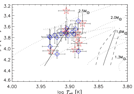
Figure 1: The positions of the selected candidate $\gamma$ Dor (star symbols) and hybrid (diamonds) stars. The parameters of the stars were taken from Huber et al. (2014). The theoretical instability strips of the $\gamma$ Dor (dashed lines) and $\delta$ Sct (solid lines) stars were taken from Dupret et al. (2005). The evolutionary tracks (Z = 0.02) were adopted from Kahraman Aliçavuş et al. (2016).

In this study, a new spectroscopic survey of a selected sample of hot $\gamma$ Dor  and hybrid stars is presented. We focused on the candidate $\gamma$ Dor  and hybrid stars located close to the hot border of the $\delta$ Sct  instability strip. We aim to answer the following questions. First, are the $T_{\rm eff}$  values of these hot objects correct? Second, do the hot $\gamma$ Dor  stars have hotter A- or B-type companions? Third, are the hybrid stars members of binary or multiple systems? Can those hot variables be rapidly-rotating stars? Additionally, are hot $\gamma$ Dor  and hybrid stars chemically peculiar? Therefore, we present a detailed spectroscopic analysis to determine the atmospheric parameters ($T_{\rm eff}$, surface gravity $\log g$, and microturbulence velocity $\xi$), projected rotatinal velocities, binarity effects, and surface chemical abundances.

The target selection is described in Sect. 2. The spectroscopic observations, data reduction and normalisation in Sect. 3. The determinations of the atmospheric parameters from photometric indices, spectral energy distribution (SED), the analysis of Balmer and metal lines are discussed in Sect. 4. The chemical abundance analysis is presented in Sect. 5. The frequency analysis of the targets is performed in Sect. 6. The discussion and conclusions are given in Sects. 7 and 8, respectively.

2 Target Selection

We started the selection process from the $\gamma$ Dor  and hybrid star candidates listed in the study of Uytterhoeven et al. (2011). They were proposed on the basis of their Kepler light curves and preliminary atmospheric parameters listed in the KIC. To better characterize them, we used the improved parameters reported in the revised Kepler catalog of Huber et al. (2014, hereafter H14), the latest available at the time of our observations (October 2016). This catalog is based on a compilation of literature values for atmospheric properties derived from a variety of observational techniques.

High-resolution spectroscopy of a well-constrained sample of stars should provide reliable answers to the questions posed in Sect. 1, especially when combining this technique with a homogeneous reduction and analysis of the spectra taken with a single instrument.

To refine our selection, we considered that the $\gamma$ Dor  stars have $T_{\rm eff}$  values in the range 6900 $-$ 7300 K (Van Reeth et al., 2015) and that the hybrid stars are expected to be found at the intersection of the $\gamma$ Dor  and $\delta$ Sct  instability strips, where $T_{\rm eff}$  changes approximately from 6600 to 7300 K. Given that the typical $T_{\rm eff}$  uncertainty is $\sim$300 K (Niemczura et al., 2017) and hot $\gamma$ Dor  stars definition by Balona et al. (2016), we selected $\gamma$ Dor  and hybrid candidates with $T_{\rm eff}$ $\geq$ 7500 K.

In the end, our selection contained nine hot $\gamma$ Dor  and fifteen hot hybrid candidate stars (Table 1), for which high-resolution spectroscopy was not available. Some of them were observed with low-resolution spectroscopy (Frasca et al., 2016; Balona et al., 2016), but it is not possible to obtain reliable $\log g$  and metallicity values from this technique.

The positions of the targets in the log $T_{\rm eff}$ $-$$\log g$  diagram are shown in Fig. 1. As can be seen from the figure, all stars are located beyond the blue edge of $\gamma$ Dor  instability strip. The $T_{\rm eff}$  values of the selected targets were also checked by using the updated parameters of the stars (Mathur et al., 2017, hereafter M17). It turned out that all targets except KIC 11508397 ($\sim$400 K cooler) still have $T_{\rm eff}$  values in the same range of the selection criteria. We used the M17 parameters in the following investigations.

3 Spectroscopic Observations

The stars were observed with the Fibre-fed Échelle Spectrograph (FIES), a cross-dispersed spectrograph mounted on the 2.56-m Nordic Optical Telescope of the Roque de los Muchachos Observatory in La Palma (Telting et al., 2014). The spectrograph offers three resolving power options. The maximum resolving power is $R$ = 67 000, while the medium and low resolving powers are $R$ = 46 000 and $R$ = 25 000, respectively, covering the wavelength range of $3700-8300$ Å.

Since we aimed to derive atmospheric parameters and chemical abundances of the targets, we opted for the medium-resolution ($R$ = 46 000) configuration, taking into account the average brightness of the sample ($V$ = 10.6 mag). Observations were performed in the first halves of the nights from October 13 to 19, 2016. To examine the binarity nature of the targets, we tried to take at least two spectra per star on different nights. For some stars, only one spectrum could be taken due to the weather conditions and the limited observing time. The number of the spectra for each star and the signal-to-noise (S/N) ratios at around 5500 Å for combined spectra are given in Table 1.

The spectra were reduced by the dedicated pipeline FIEStool (Telting et al., 2014). The standard reduction procedure was applied. Bias subtraction, correction of flat-field, scattered light extraction, wavelength calibration, and merging of orders were performed for each spectrum. Normalisation of the reduced spectra was carried out manually by using the continuum task of the NOAO/IRAF package.

Table 1: Log of the observations (from October 13 to 19, 2016): number of the star (N_i) used in the paper, KIC ID, V-magnitude, signal-to-noise ratio (S/N), number of taken spectra (N_S), and input classification (Uytterhoeven et al., 2011).

Ni	KIC	V	S/N	Ns	Input
		[mag]			classifcation
1	2168333	10.02	90	2	Hybrid
2	3119604	10.90	50	1	Hybrid
3	3231406	10.38	85	2	Hybrid
4	3240556	10.10	75	2	Hybrid
5	3245420	10.52	75	2	Hybrid
6	3868032	10.44	70	2	$\gamma$ Dor
7	4677684	10.19	85	2	$\gamma$ Dor
8	4768677	10.91	60	2	Hybrid
9	5180796	10.11	85	2	$\gamma$ Dor
10	5630362	10.69	70	2	$\gamma$ Dor
11	6199731	10.94	50	1	Hybrid
12	6500578	10.77	80	2	$\gamma$ Dor
13	6776331	10.71	50	1	Hybrid
14	7694191	10.94	45	1	$\gamma$ Dor
15	7732458	10.85	75	2	Hybrid
16	9052363	10.64	60	2	Hybrid
17	9775385	11.05	45	1	Hybrid
18	10281360	11.06	50	1	$\gamma$ Dor
19	11197934	10.81	60	2	Hybrid
20	11199412	10.90	50	1	$\gamma$ Dor
21	11508397	10.65	80	2	Hybrid
22	11612274	10.44	85	4	$\gamma$ Dor
23	11718839	10.73	60	2	Hybrid
24	11822666	10.69	70	2	Hybrid

4 Determination of the Atmospheric parameters

The spectroscopic atmospheric parameters ($T_{\rm eff}$, $\log g$, and $\xi$) were determined using the Balmer and iron lines, as done in previous several studies (e.g., Nieva & Przybilla, 2010; Tkachenko et al., 2012; Niemczura et al., 2017). The approach we used in the analysis of the Balmer lines has been successfully applied in other papers (Catanzaro et al., 2011; Catanzaro & Balona, 2012; Catanzaro, Ripepi, & Bruntt, 2013). In practice, the procedure minimized the difference between observed and synthetic spectra, using the $\chi^{2}$ as goodness-of-fit parameter. Since the rotational velocity affects the profile of the lines, we determined initial estimates of projected rotational velocity ($v\sin i$) values by using the least-squares deconvolution (LSD) technique (Donati et al., 1997). The $v\sin i$  values were measured from the zero positions of the Fourier transform of the mean line profiles (Table 1).

Table 2: The atmospheric parameters taken from M17 and our $T_{\rm eff}$ values derived from the analysis of Balmer lines. ${\it E(B-V)}$ values (Sect. 7.6) are also listed.

Number	KIC	$E(B-V)$	$T_{\rm eff}$M17	$\log g$M17	$T_{\rm eff}$Hlines
		[mag]	[K]	[dex]	[K]
		$\pm$ 0.02
1	2168333	0.03	8363${}^{+197}_{-395}$	3.80${}^{+0.36}_{-0.15}$	8000 $\pm$ 300
2	3119604	0.03	8383${}^{+233}_{-350}$	4.10${}^{+0.14}_{-0.15}$	7900 $\pm$ 360
3	3231406	0.02	8005${}^{+222}_{-333}$	3.77${}^{+0.40}_{-0.07}$	7600 $\pm$ 270
4	3240556	0.03	8615${}^{+238}_{-374}$	3.78${}^{+0.41}_{-0.14}$	8000 $\pm$ 300
5	3245420	0.11	8079${}^{+225}_{-338}$	3.72${}^{+0.43}_{-0.11}$	7900 $\pm$ 320
6	3868032	0.10	8564${}^{+234}_{-402}$	4.04${}^{+0.16}_{-0.16}$	8300 $\pm$ 610
7	4677684	0.22	8602${}^{+68}_{-94}$	3.78${}^{+0.28}_{-0.11}$	8600 $\pm$ 480
8	4768677	0.20	8584${}^{+77}_{-86}$	3.76${}^{+0.26}_{-0.03}$	8800 $\pm$ 830
9	5180796	0.15	8076${}^{+64}_{-96}$	3.82${}^{+0.22}_{-0.09}$	8100 $\pm$ 280
10	5630362	0.11	7821${}^{+78}_{-78}$	3.88${}^{+0.17}_{-0.07}$	7700 $\pm$ 170
11	6199731	0.05	8040${}^{+251}_{-306}$	3.64${}^{+0.55}_{-0.09}$	7500 $\pm$ 320
12	6500578	0.28	8072${}^{+223}_{-363}$	3.72${}^{+0.42}_{-0.10}$	8200 $\pm$ 450
13	6776331	0.08	7870${}^{+244}_{-325}$	3.70${}^{+0.46}_{-0.08}$	7600 $\pm$ 400
14	7694191	0.19	8070${}^{+251}_{-334}$	3.66${}^{+0.50}_{-0.09}$	8300 $\pm$ 580
15	7732458	0.02	7766${}^{+216}_{-324}$	3.64${}^{+0.49}_{-0.09}$	7300 $\pm$ 230
16	9052363	0.11	7810${}^{+216}_{-324}$	3.74${}^{+0.42}_{-0.10}$	7800 $\pm$ 360
17	9775385	0.05	7675${}^{+211}_{-316}$	4.05${}^{+0.17}_{-0.15}$	7300 $\pm$ 300
18	10281360	0.06	7776${}^{+216}_{-325}$	4.02${}^{+0.22}_{-0.14}$	7200 $\pm$ 280
19	11197934	0.06	7641${}^{+68}_{-91}$	3.83${}^{+0.22}_{-0.06}$	7600 $\pm$ 360
20	11199412	0.02	7693${}^{+239}_{-319}$	3.72${}^{+0.46}_{-0.08}$	7200 $\pm$ 280
21	11508397	0.00	7287${}^{+76}_{-87}$	3.87${}^{+0.18}_{-0.10}$	7200 $\pm$ 240
22	11612274	0.00	7694${}^{+214}_{-322}$	3.60${}^{+0.54}_{-0.06}$	7000 $\pm$ 190
23	11718839	0.03	8443${}^{+233}_{-367}$	3.76${}^{+0.42}_{-0.14}$	8100 $\pm$ 500
24	11822666	0.03	8615${}^{+238}_{-374}$	3.78${}^{+0.42}_{-0.14}$	8200 $\pm$ 540

Synthetic spectra were generated in three steps. First, we computed LTE atmospheric models using the ATLAS9 code (Kurucz, 1993a, b). Second, the stellar spectra were then synthesized using SYNTHE (Kurucz & Avrett, 1981). Third, the spectra were convolved with the instrumental and rotational broadenings.

$T_{\rm eff}$  was estimated by computing the ATLAS9 model atmosphere which gave the best match between the observed $H_{\alpha}$, $H_{\beta}$, $H_{\gamma}$, and $H_{\delta}$ lines profile and those computed with SYNTHE. The models were computed using solar opacity distribution functions (ODF). It is also known that Balmer lines are not sensitive to $\log g$  parameter for $T_{\rm eff}$ $\lesssim$ 8000 K (Smalley et al., 2002). Considering the $T_{\rm eff}$  range of our targets and the error bars, we fixed the $\log g$  and metallicity values to 4.0 dex and solar, respectively.

The Balmer lines are located far from the edges of the échelle orders. The simultaneous fitting of four lines led to a final solution at the intersection of the four $\chi^{2}$ iso-surfaces. An important source of uncertainty arose from difficulties in the normalization since it is always challenging for Balmer lines in échelle spectra. The uncertainties on the $T_{\rm eff}$  values were estimated by introducing a 1$\sigma$ change in the normalization level and a 0.2 dex error on $\log g$  and metallicity. We also considered the errors on the initial $v\sin i$  values (Table 1). These uncertainties were summed in quadrature with the errors obtained by the fitting procedure. The final results for $T_{\rm eff}$  values and their errors are reported in Table 2.

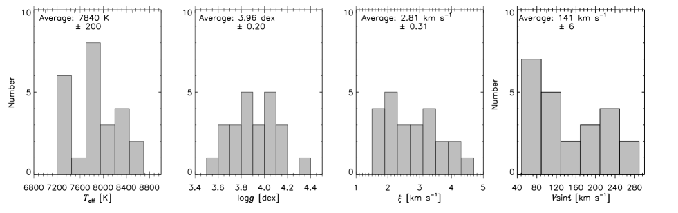
Figure 2: Distributions of the final atmospheric parameters determined from the iron lines analysis and $v\sin i$  values.

Final atmospheric parameters were derived by using the excitation and the ionisation potentials of metal lines. For the correct atmospheric parameters of a star, all lines of the same element should give the same chemical abundance. The relationship between the chemical abundance and the excitation, ionisation potentials of the same element should be flat.

We used Fe lines in the analysis, since they are the most numerous lines in the spectra having the $T_{\rm eff}$  range of our stars. The ATLAS9 (Kurucz, 1993a, b) model atmospheres were synthesized by using the SYNTHE code (Kurucz & Avrett, 1981) in this and the following chemical abundance analysis. A synthetic spectrum is adjusted until it fits well the observed spectrum looking at $\chi^{2}$ parameter (for more details see Niemczura et al. 2015, Kahraman Aliçavuş et al. 2016). The Fe lines of all stars were analysed for a range of $T_{\rm eff}$, $\log g$, and $\xi$ with a step of 100 K, 0.1 dex and 0.1 km s^-1, respectively. The range of the atmospheric parameters was selected taking into account the initial $T_{\rm eff}$  values derived from Balmer lines and the values given by M17 (Table 2). After the analysis was performed, we determined $T_{\rm eff}$  and $\log g$  values considering the excitation potential$-$abundance and the ionisation potential$-$abundance relations, respectively. The $\xi$ values were also obtained by checking the dependence between abundance and line strength. The obtained atmospheric parameters are given in Table 3. The uncertainties in the parameters were estimated by checking how much the parameters change for $\sim$$5$ % differences in the excitation potential$-$abundance, ionisation potential$-$abundance, and the abundance$-$line strength relationships.

The distributions of the derived atmospheric parameters are shown in Fig. 2. The final $T_{\rm eff}$, $\log g$, and $\xi$ ranges were obtained to be $7200-8600$ K, $3.5-4.4$ dex, and $1.5-4.4$ km s^-1, respectively. The final atmospheric parameters were compared with the M17 atmospheric parameters. In most cases $T_{\rm eff}$  values are consistent with each other within errors. However, in Fig. 3, the final $\log g$  values were also compared with the $\log g$  values given by M17. The final $\log g$  values are generally higher than the M17 $\log g$  values for the $T_{\rm eff}$  ranges of our stars. Additionally, it appears that the $\log g$  difference between our spectroscopic values and M17 ones increases with the growing $\log g$. The relationship between those parameters is shown in the lower panel of Fig. 3.

Figure 3: Differences between the final spectroscopic $\log g$  and the $\log g$  taken from M17 as a function of the final spectroscopic $T_{\rm eff}$  (upper panel) and $\log g$  (lower panel) obtained from the iron line analysis. Dashed lines represent 1-$\sigma$ levels. The Spearman’s rank correlation coefficient (R) and probability (the number after comma) are given in the right corner of the right panel.

Relations between $\xi$ and $T_{\rm eff}$  and $\log g$  were checked as shown in Fig. 4. The $\xi$ $-$ $T_{\rm eff}$  relationship has already been examined in several studies (e.g., Landstreet et al., 2009; Gebran et al., 2014; Niemczura et al., 2017). According to these studies, a decline in $\xi$ is expected for the $T_{\rm eff}$  value higher than about 7000 K. The $\xi$ $-$ $\log g$  relationship was also examined by Gray, Graham, & Hoyt (2001). They showed a relation between these two parameters for spectral types from A5 to G2. According to this relation, the $\xi$ values decrease with increasing $\log g$. However, as our sample spans a $T_{\rm eff}$  range narrower than the A5 $-$ G2 one, we could not verify these relationships (Fig. 4).

Figure 4: The final $\xi$ as a function of the final spectroscopic $T_{\rm eff}$  (right panel) and $\log g$  (left panel).

Table 3: The final atmospheric parameters derived from the iron lines analysis, the $v\sin i$  values and the Fe abundances. The final pulsation type classification is given in last column as a result of our frequency analysis.

Number	KIC	$T_{\rm eff}$	$\log g$	$\xi$	$\log\epsilon$ (Fe)	$v\sin i$	Pulsation
		[K]	[dex]	[km s-1]	[dex]	[km s-1]	type
1	2168333	8400 $\pm$ 200	3.7 $\pm$ 0.2	2.0 $\pm$ 0.5	7.47 $\pm$ 0.27	175 $\pm$ 9	$\delta$ Sct
2	3119604	7700 $\pm$ 200	3.9 $\pm$ 0.3	2.9 $\pm$ 0.2	7.23 $\pm$ 0.34	92 $\pm$ 5	$\delta$ Sct
3	3231406	7900 $\pm$ 100	3.8 $\pm$ 0.2	2.1 $\pm$ 0.2	7.63 $\pm$ 0.31	169 $\pm$ 10	Hybrid
4	3240556	7800 $\pm$ 200	4.4 $\pm$ 0.2	1.5 $\pm$ 0.5	7.51 $\pm$ 0.35	213 $\pm$ 9	$\delta$ Sct
5	3245420	8100 $\pm$ 200	3.7 $\pm$ 0.1	2.0 $\pm$ 0.2	7.58 $\pm$ 0.32	151 $\pm$ 6	$\delta$ Sct
6	3868032	8400 $\pm$ 200	4.0 $\pm$ 0.3	3.5 $\pm$ 0.4	7.11 $\pm$ 0.32	181 $\pm$ 9	Non-pulsator
7	4677684	8500 $\pm$ 200	3.5 $\pm$ 0.2	1.7 $\pm$ 0.3	7.52 $\pm$ 0.28	71 $\pm$ 3	$\gamma$ Dor
8	4768677	8600 $\pm$ 300	4.2 $\pm$ 0.3	2.0 $\pm$ 0.5	6.94 $\pm$ 0.50	256 $\pm$ 14	$\delta$ Sct
9	5180796	8400 $\pm$ 200	4.0 $\pm$ 0.2	2.5 $\pm$ 0.2	7.73 $\pm$ 0.30	152 $\pm$ 6	$\gamma$ Dor
10	5630362	7700 $\pm$ 300	3.7 $\pm$ 0.3	3.0 $\pm$ 0.5	7.34 $\pm$ 0.33	230 $\pm$ 12	$\gamma$ Dor
11	6199731	7800 $\pm$ 200	4.1 $\pm$ 0.3	4.4 $\pm$ 0.4	7.23 $\pm$ 0.35	236 $\pm$ 10	$\delta$ Sct
12	6500578	7700 $\pm$ 300	3.8 $\pm$ 0.2	1.9 $\pm$ 0.3	7.35 $\pm$ 0.30	95 $\pm$ 6	$\gamma$ Dor
13	6776331	7900 $\pm$ 200	3.9 $\pm$ 0.1	2.3 $\pm$ 0.2	7.65 $\pm$ 0.32	49 $\pm$ 3	Hybrid
14	7694191	8400 $\pm$ 200	4.1 $\pm$ 0.2	3.9 $\pm$ 0.2	7.31 $\pm$ 0.36	76 $\pm$ 6	$\gamma$ Dor
15	7732458	7800 $\pm$ 200	4.1 $\pm$ 0.2	2.6 $\pm$ 0.2	7.73 $\pm$ 0.34	87 $\pm$ 5	$\delta$ Sct
16	9052363	8000 $\pm$ 200	4.1 $\pm$ 0.2	3.5 $\pm$ 0.3	7.40 $\pm$ 0.33	109 $\pm$ 5	Non-pulsator
17	9775385	7400 $\pm$ 200	4.2 $\pm$ 0.2	4.1 $\pm$ 0.2	7.44 $\pm$ 0.36	71 $\pm$ 3	Hybrid
18	10281360	7200 $\pm$ 200	4.2 $\pm$ 0.2	4.1 $\pm$ 0.3	7.29 $\pm$ 0.36	108 $\pm$ 5	$\gamma$ Dor
19	11197934	7600 $\pm$ 200	3.9 $\pm$ 0.2	3.0 $\pm$ 0.5	7.46 $\pm$ 0.31	267 $\pm$ 18	Hybrid
20	11199412	7200 $\pm$ 200	4.1 $\pm$ 0.2	3.9 $\pm$ 0.3	6.68 $\pm$ 0.35	77 $\pm$ 6	$\gamma$ Dor
21	11508397	7200 $\pm$ 200	3.9 $\pm$ 0.3	1.5 $\pm$ 0.5	7.68 $\pm$ 0.30	240 $\pm$ 11	Hybrid
22	11612274	7400 $\pm$ 200	3.8 $\pm$ 0.1	3.2 $\pm$ 0.2	7.38 $\pm$ 0.27	130 $\pm$ 7	$\gamma$ Dor
23	11718839	8100 $\pm$ 200	3.9 $\pm$ 0.1	3.4 $\pm$ 0.2	7.45 $\pm$ 0.32	57 $\pm$ 3	$\delta$ Sct
24	11822666	8200 $\pm$ 200	4.0 $\pm$ 0.1	2.5 $\pm$ 0.2	7.37 $\pm$ 0.31	115 $\pm$ 7	Hybrid

5 Analysis of chemical abundances

Chemical abundances of the stars were derived by performing spectrum synthesis. The derived atmospheric parameters were taken as input during the analysis and the chemical abundances of individual elements were determined in addition to $v\sin i$.

In the first step of the analysis, all lines in the spectra were divided into subsets line by line. In the case of rapidly rotating stars, lines are mostly blended. Therefore, for rapidly rotating stars wider ranges in wavelength were selected considering the normalisation level. For each subset the line identifications were done by using the line list of Kurucz. Then these spectral subsets were analysed separately. The identified elements in each spectral subset and $v\sin i$  values were adjusted during the analysis. Taking the minimum difference between the observed and theoretical spectra, chemical abundances and $v\sin i$  values were obtained from each spectral subset. The range of $v\sin i$  was found to be from 49 to 267 km s^-1  (Table 3, Fig. 2).

The average values of the abundances of individual elements for each star are given in Table 3 and the uncertainties given in this table are the standard deviations. The total uncertainties were estimated by considering the errors in the obtained atmospheric parameters, assumptions in the model atmospheres, the resolution and the S/N ratio of spectra (Kahraman Aliçavuş et al., 2016). As a result, the uncertainty in the obtained abundances was found to be 0.28 dex on average. The total uncertainties were estimated for the Fe abundances (Table 3).

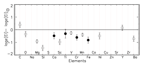
Figure 5: Differences between the derived chemical abundances and the Solar values (Asplund et al., 2009) as a function of elements for KIC 11199412. Filled circles show the differences that were obtained from at least 5 and more lines, while others represent the opposite.

Figure 6: Differences between the spectroscopic [Fe/H] and [Fe/H] taken from H14 as a function of the spectroscopic [Fe/H] (left panel) and $T_{\rm eff}$  (right panel). The Spearman’s rank correlation coefficient (R) and probability (the number after comma) are given in the right corner of the right panel.

Consequently, we found that all stars have chemical abundances similar to solar (Asplund et al., 2009). There are three stars, KIC 3868032, KIC 4768677 and KIC 11199412, which seem to have moderately underabundant Fe ([Fe/H] $\lesssim$  $-$ 0.50 dex). However, when the uncertainties in Fe abundances of these stars were considered, we can say that only KIC 11199412 has slightly lower Fe abundance. Additionally, this star displays underabundance in almost all elements compared to the solar abundances (Fig. 5). We compared our [Fe/H] values and the values given by M17 (Fig. 6). According to the right panel, the difference between the spectroscopic [Fe/H] and the [Fe/H] values given by M17 increases after [Fe/H]=0.0 dex. However, the Spearman’s rank coefficient R do not support the significance of such a trend: the correlation coefficient of $R=0.22$ and a probability value 0.31 indicate that there is no significant correlation.

Finally, KIC 11199412 clearly shows weak metal and Ca ii K lines. KIC 11718839 also exhibits slightly weaker metal and Ca ii K lines comparing the hydrogen spectral type, but not enough to classify it as a peculiar star. For sake of completeness, we report our final supervised spectral classification in Table 1.

6 Frequency analysis of photometric data

To precisely classify the pulsational behaviour of the selected targets, we performed an independent frequency analysis of the Kepler data. The original time series were retrieved from the MAST archive. Keeping the subdivision into long- and short-cadence acquisition mode, the original data were normalized to the mean values of each quarter, thus correcting instrumental drifts. During this procedure isolated outliers were removed. When reconstructing the pulsational content of our variables, we used the short-cadence time series to investigate the region above the Nyquist frequency ($f$ = 24.5 d^-1) of the more numerous long-cadence data.

The accurate time series were then analysed for their constituent frequencies with the goal to establish their modal content. We have used the iterative both sine-wave fitting method (Vaniĉek 1971) and the software package Period04 (Lenz & Breger, 2005). The final goal is to determine the pulsational characteristics with respect to the spectroscopic properties and the position in the H-R diagram. The initial variability classification of our targets ($\gamma$ Dor, hybrid) was taken from Uytterhoeven et al. (2011). When our analysis was almost finished, Murphy et al. (2019) used Gaia–derived luminosities to propose another classification scheme based on the skewness of the amplitudes in the Fourier spectra. However, these authors focused on the $\delta$ Sct  stars, without investigating the frequency region below 5 d^-1, where $\gamma$ Dor  and hybrid stars are expected to show their $g$-modes.

6.1 Variability not induced by pulsation

The most obvious case was that of KIC 3868032. The frequency spectrum clearly shows peaks at $f$ = 0.40 d^-1, 2$f$, 3$f$, and 4$f$. The spectroscopic analysis pointed out a mean profile with two superimposed components, with clearly different rotational regimes, i.e., $v\sin i$ = 180 km s^-1  and $v\sin i$ $<100$ km s^-1. Uytterhoeven et al. (2011) classified it as a $\gamma$ Dor  variable. However, these peaks are associated with the orbital motion and cannot be ascribed to pulsation. We noticed that after considering $f$ and harmonics, a peak at $f_{1}$ = 1.68 d^-1  appears, close but not equal to 4$f$. It could be still an artifact of the orbital/rotational effects, but its pulsational origin cannot be ruled out.

The case of KIC 9052363 is similar. The light curve is almost flat, without any clear feature that could be ascribed to pulsation. The frequency analysis reveals a couple of low-frequency, very-low amplitude peaks. Due to their incoherence, small rotational effects are the most plausible reason. Both stars are also reported as non-$\delta$ Sct  by Murphy et al. (2019).

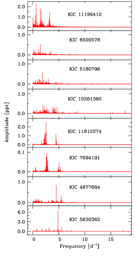
Figure 7: Amplitude spectra obtained by combining short- and long-cadence data of the variables showing a regime of low-frequency ($f\leq 6$ d^-1) modes. They are ordered for increasing frequency of the highest peak.

6.2 Low-frequency regime

Eight stars in our sample show a set of low-frequency peaks only. We ordered them by increasing frequency of the strongest peak (Fig. 7). We note that the range of frequencies is small, not exceeding 6 d^-1. Occasional high frequency peaks appear in the frequency spectra not enough to claim that a clear double regime of pulsation is present. It is noteworthy that all stars in Fig. 7  were classified as $\gamma$ Dor  by Uytterhoeven et al. (2011). Actually, they are the only stars classified as $\gamma$ Dor  in our sample and therefore we are in full agreement.

KIC 5630362 is the star showing the highest frequency ($f$ = 4.856 d^-1, $P$ = 0.206 d), with an amplitude much larger than those of the others (bottom panel). It is unlikely that this frequency is that of the fundamental radial mode, since the long period would suggest an evolved $\delta$ Sct  star: the very fast rotation (230 km s^-1) and the gravity ($\log g$ = 3.7 dex) do not support such an hypothesis. Therefore, pulsators with largely predominant modes also exist in $\gamma$ Dor  stars, not only in $\delta$ Sct  ones (i.e., the Group A proposed by Murphy et al. 2019).

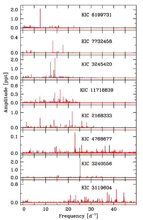
Figure 8: Amplitude spectra obtained by combining short- and long-cadence data of the variables showing a prevailing regime of high-frequency modes. They are ordered for increasing frequency of the highest peak.

6.3 High-frequency regime

None of the stars in our sample was classified as a pure $\delta$ Sct  star. However, our frequency analysis showed that some stars are characterized by a large set of high-frequency peaks accompanied by no (or a few) low-frequency ones (Fig. 8). The case of KIC 3240556 is noteworthy, since this star shows a largely predominant mode. The frequency is too high ($f$ = 25.2 d^-1) to be due to rotation. Note that the short-cadence time series allowed us to determine the exact value of this high frequency very close to the Nyquist frequency of the long-cadence data. KIC 3240556 surely belongs to Group A in the Murphy et al. (2019) classification scheme.

All these variables were classified as hybrid stars. However, we know from the analysis of line-profile variations that very high-degree modes (up to $\ell$=14) are excited in $\delta$ Sct  stars and they are spectroscopically detectable (Poretti et al., 2009; Mantegazza et al., 2012). The rotational splitting can shift the frequencies of retrograde modes of multiplets toward low values, thus producing the bunch of peaks observed there in hybrid stars. They also could be combination terms between high-frequency modes or again effects of the rotational modulation induced by changing spots and/or faculae on the stellar surfaces. We emphasize that in general this multiplicity of causes does not make a few low-frequency peaks on their own a sufficient criterion to claim for an hybrid pulsational regime.

6.4 Low and high-frequency regime

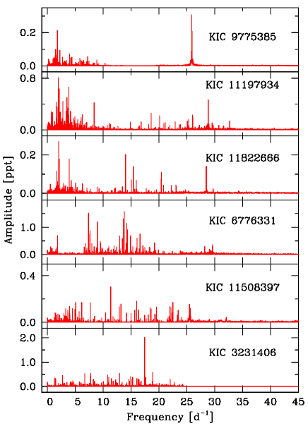
Figure 9: Amplitude spectra obtained by combining short- and long-cadence data of the variables showing clear regimes of both high-frequency and low-frequency peaks.

Only six stars show simultaneously well-defined low- and high-frequency regimes (Fig. 9), with clear peaks in both regions. However, it has to be noted how the amplitude spectra differ: there are low- and high-frequencies both confined in separated groups and continuously distributed. All these stars had an input classification as hybrid variables.

7 Discussion

We can now use the results from the frequency and atmospheric analyses to better define the properties of our targets and closely look at how much they are really peculiar, as suggested by previous works. Our new classification and parameters are reported in Table 3. In the left panel of Fig. 10, the log $T_{\rm eff}$ $-$$\log g$  positions are shown on the basis of the predicted atmospheric parameters by M17, while in the right panel our final atmospheric parameters are used. As can be noticed, the larger changes in the positions are mostly due to the differences in the $\log g$  values.

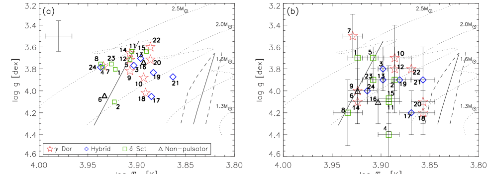
Figure 10: a) The positions of the target stars, as numbered in Table 3, according to the atmospheric parameters given by M17. b) The positions of the stars according to the final atmospheric parameters. The theoretical instability strips of the $\gamma$ Dor (dashed-lines) and $\delta$ Sct (solid lines) stars were taken from Dupret et al. (2005). The evolutionary tracks (Z=0.02) were adopted from Kahraman Aliçavuş et al. (2016).

7.1 Binary nature

Composite spectra suggesting double-lined spectroscopic binaries are not observed, except for the ellipsoidal variable KIC 3868032 (Sect. 6.1). Seventeen stars in our sample have at least two spectra taken on different nights. The radial velocities were examined: if there was a companion, the radial velocities should vary due to the orbital motion. We did not find any large variation in the radial velocities. Nevertheless, the very small number of observations and their very limited time coverage do not allow us to clearly detect long-period or small-amplitude or low-inclination binary systems. For example, KIC 2168333 and KIC 11508397 are known binaries with very long orbital periods ($\gtrsim$ 350 d; Murphy et al., 2018), but the radial velocities obtained from their two spectra differ by 2.6 and 1.5 km s^-1 only, respectively.

7.2 Pulsation characteristics vs new atmospheric parameters

Our detailed frequency analysis was able to clean the physical scenario since 10 targets (8 $\delta$ Sct  and 2 non-pulsating stars; Sects. 6.1 and  6.2, respectively) out of 24 (42%) can be retired from the initial sample of $\gamma$ Dor  and hybrid pulsators. In particular the 8 $\delta$ Sct  stars erroneously classified as hybrid variables turned out to be normal $p$-modes pulsators, well inside the $\delta$ Sct  instability strip. Additionally, the two non-pulsators remain located close to the hot border of the $\delta$ Sct  domain, where the fraction of $\delta$ Sct  pulsating stars is estimated to be $\sim$40% (Murphy et al., 2019).

Among the six hybrid variables, only KIC 11822666 is really a hot star (8200 K), while the $T_{\rm eff}$  of KIC 9775385, KIC 11197934, and KIC 11508397 are very close or below the 7300 K limit when taking into account the error bars. KIC 6776331 and KIC 3231406 have intermediate values (7900 K).

A similar count applies to the 8 targets re-classified as pure $\gamma$ Dor  stars: five (KIC 5630362, KIC 6500578, KIC 10281360, KIC 11199412, and KIC 11612274) have $T_{\rm eff}$  values in agreement with that of the hot border of the classical $\gamma$ Dor  strip (assuming 1$\sigma$ error bars), though KIC 5630362 and KIC 6500578 seem to be more luminous than usual for $\gamma$ Dor  stars (Fig. 12). Note that the normal $\gamma$ Dor  pulsator KIC 11199412 is the only star showing hints of chemical peculiarities (Sect. 7.4). In three cases (KIC 4677684, KIC 7694191, and KIC 5180796) the $T_{\rm eff}$  values are well above 8000 K.

In the end, we have 8 stars (3 hybrid and 5 normal $\gamma$ Dor  pulsators) that show $g$-modes even if they are beyond the hot border of the $\gamma$ Dor  instability strip: namely, KIC 3231406, KIC 6776331, KIC 11822666, KIC 4677684, KIC 5180796, KIC 5630362, KIC 6500578, and KIC 7694191. They constitute our final bona-fide sample. We recall that the whole initial sample (24 stars) was expected to be composed of such unusual $\gamma$ Dor  pulsators.

7.3 Other atmospheric parameters

When the obtained atmospheric parameters are taken into account, most stars are found that they have $T_{\rm eff}$  values in agreement with those given by M17. Only two stars, KIC 10281360 and KIC 11199412, show spectroscopic $T_{\rm eff}$  values about 500 K cooler than the previously given values by M17. This explains why the previous classification put them so close to the hot border.

Our final $\log g$  values were compared with the $\log g$  values given by M17 (Fig. 3). In some cases, the final $\log g$ values differ more than 0.4 dex. Therefore, the positions of these stars change in the log $T_{\rm eff}$ $-$$\log g$  diagram (Fig. 10). When taking into account the final positions in the log $T_{\rm eff}$ $-$$\log g$  diagram and the evolutionary tracks, we can say that $\sim$$70$ % of stars have masses from 2.0 to 2.5 $M_{\sun}$, while the mass range of the others is between 1.6 and 2.0 $M_{\sun}$.

The microturbulent velocity $\xi$ changes with $T_{\rm eff}$  (Gray, Graham, & Hoyt, 2001; Smalley, 2004; Landstreet et al., 2009) and the $\xi$ value varies from $\sim$1.5 to 3 km s^-1  for $T_{\rm eff}$  range of about 7000 $-$ 7300. However, three cool stars (KIC 9775385, KIC 10281360, KIC 11199412) have $\xi$ values between 3.9 and 4.1 km s^-1with a maximum uncertainty of 0.3 km s^-1. These $\xi$ values are high for this $T_{\rm eff}$  range, but the three stars seem to be normally located on the cool border of the $\gamma$ Dor  instability strip. For the other hotter stars the $\xi$ range is between 1.5 and 4.5 ($\pm$ 0.3) km s^-1, as expected for A-type stars.

Some target stars have low-resolution LAMOST spectroscopy in the literature. The atmospheric parameters derived from these studies are given in Table 2. When we compared these results with our final atmospheric parameters, we found significant differences and trends between the parameters obtained from the high- and low-resolution spectroscopy (Fig. 11).

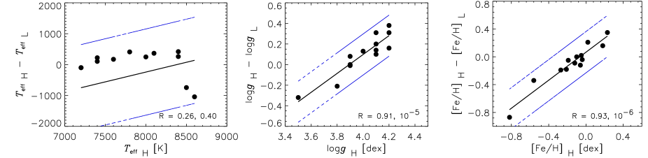
Figure 11: Comparison of the atmospheric parameters obtained from high- and low-resolution spectroscopy. The subscripts $H$ and $L$ defines the high- and low-resolution spectroscopy, respectively. The Spearman’s rank correlation coefficient (R) and probability (the number after comma) are given in the right corner of the panels. Blue lines represent the 1$\sigma$ levels.

7.4 Chemical abundances

Anomalous abundances, like the Am phenomenon (Hareter et al., 2011), have been considered a possible physical explanation of the hybrid $\gamma$ Dor-$\delta$ Sct  pulsation. Our analysis did not reveal any abundance peculiarity in our bona-fide sample of eight hot $\gamma$ Dor  and hybrid stars, in agreement with recent studies showing that most hybrid stars are chemically normal (Niemczura et al., 2015, 2017). We also searched for He lines, without any significant detection. Only KIC 11199412 (a normal $\gamma$ Dor  star) exhibits a moderate underabundance in almost all the elements (Fig. 5).

7.5 The $v\sin i$  values and the SPB hypothesis

It has been suggested that hot $\gamma$ Dor  stars are actually rapidly-rotating SPB stars (Salmon et al., 2014; Balona et al., 2015). Due to gravity darkening, their equatorial zones appear cooler than the rest of the surface, then they are classified as hot A-stars and, hence, as hot $\gamma$ Dor  variables.

Balona et al. (2016) determined an average $v\sin i$ = 114 km s^-1  for a group of six hot $\gamma$ Dor  stars. Our five bona-fide hot $\gamma$ Dor  stars show $v\sin i$  values ranging from 71 to 230 km s^-1  (Table 3), with an average value of 125 km s^-1. In the spectral range B5-B9, main-sequence stars, like SPB variables, show a mean $v\sin i$ = 144 km s^-1  (Głȩbocki & Gnaciński, 2005; Balona et al., 2016). Since hot $\gamma$ Dor  stars do not seem to rotate faster than normal SPB stars, they do not constitute a special SPB subclass. Moreover, we could not find spectral lines indicative of the B-type (Sect. 7.4), which should be present at least for SPB stars seen at intermediate or pole-on orientations. Finally, gravity darkening does not seem to be able to lower the $T_{\rm eff}$  of SPB stars sufficiently to approach the hot border of the $\delta$ Sct instability strip (see Fig. 4 in Salmon et al., 2014). We prudently note that the classification as hot or classical hybrid/$\gamma$ Dor  stars could also be affected by the gravity darkening, especially in case of fast rotators seen almost equator-on, like KIC 5630362, KIC 11197934, and KIC 11508397.

7.6 Gaia parallaxes

As a final check, we used the Gaia parallaxes (Gaia Collaboration et al., 2018) to investigate the positions of the stars in the H-R diagram. We adopted the bolometric corrections computed taking into account the $T_{\rm eff}$  values (Flower, 1996). The extinction coefficients ($A$_V) were estimated using the interstellar reddening $E(B-V)$ values (Table 2). These were obtained by measuring the equivalent widths of the Na D lines in our spectra and then applying the relation given by Munari & Zwitter (1997).

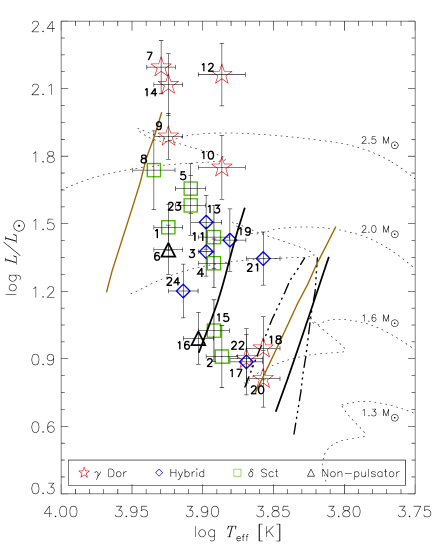
Figure 12: The positions of the stars in the H-R diagram, as numbered in Table 1. The theoretical instability strips of the $\gamma$ Dor (dashed-lines) and $\delta$ Sct (solid black lines) stars were taken from Dupret et al. (2005). The recently suggested $\delta$ Sct  instability strip (Murphy et al., 2019) is shown by brown solid lines. The evolutionary tracks (Z=0.02) were adopted from Kahraman Aliçavuş et al. (2016).

An offset of $-0.03$ mas in the Gaia parallaxes was found (Lindegren et al., 2018; Zinn et al., 2019). However, when this offset was applied to a large sample ($\sim$ 15000 stars), a huge amount of stars goes below the zero-age main-sequence with unreasonably low luminosities (Murphy et al., 2019). Therefore, to calculate our final Gaia luminosities we did not apply this offset to the parallaxes, accordingly with recent studies (Arenou et al., 2018; Murphy et al., 2019). The positions of the stars in the H-R diagram are illustrated in Fig. 12. Note that the new empirical instability strip of $\delta$ Sct  stars (Murphy et al., 2019) now incorporates some variables located beyond the hot border of the previous theoretical instability strip.

As can be noticed from Fig. 12, stars 7, 9, 10, 12, and 14 (see Table 3 for their KIC identification) have very high luminosities. When the radii of those hot $\gamma$ Dor  stars were calculated using the Gaia luminosities, we obtained values ranging from 4.3 to 6.0 $R_{\odot}$. We also calculated the radii of the hot $\gamma$ Dor  stars classified by Balona et al. (2016). It turned out that $\sim$70% of their sample have larger radii (3.2 $<$ $R_{\odot}$ $<$ 7.2). Main-sequence A-F type stars should have radii in the range $1.5-2.7$ $R_{\odot}$ (Cox, 2000). Therefore, the larger size of the hot $\gamma$ Dor  pulsators appears to support the hypothesis that they are different from main-sequence A-F pulsators. They could be evolved A-F stars or more massive stars (such as B-type stars) entering the classical instability strip in their redward evolution. The impact of enhanced iron opacity on stellar pulsations can lead to a substantial revision of the instability strips (Moravveji, 2016) and then play a key role to explain the location of our hot hybrid and $\gamma$ Dor  variables. Additionally, the higher luminosity values of these hot stars may be the result of binarity. These systems could be a member of a long orbital period binary system which could not detect with our present spectroscopic data.

8 Conclusions

We performed a detailed spectroscopic and photometric study of a group of 24 Kepler targets, all claimed to be hot $\gamma$ Dor  or $\delta$ Sct-$\gamma$ Dor  hybrid stars, located well beyond the theoretical $\gamma$ Dor  instability strip (Uytterhoeven et al., 2011). The detailed frequency analysis of the Kepler time series and the determination of $T_{\rm eff}$  and other atmospheric parameters performed with the new FIES spectra allowed us to set the bona-fide sample of such peculiar pulsators to five hot $\gamma$ Dor  stars and three hot hybrid stars. If on one hand we provide a strong confirmation that these peculiar pulsators exist, on the other we reduce their recurrence to 1/3 to what originally evaluated. Therefore, we can assume that the physical explanation should reside in a mechanism or a cause applicable to a limited number of stars, not to the vast majority of the $\delta$ Sct  or $\gamma$ Dor  variables.

Searching for this still elusive explanation, we did not find any peculiarity in the atmospheric parameters and chemical abundances. The lack of composite spectra does not support the possibility that the hot hybrid stars are binaries in which one or both components are normal $\delta$ Sct  and/or $\gamma$ Dor  pulsators. We investigated the rotation rate and we cannot support the hypothesis that hot $\gamma$ Dor  pulsators are actually fast-rotating SPB stars. On the other hand, Gaia luminosities suggested us that hot $\gamma$ Dor  pulsators have larger radii and higher luminosities than normal main sequence A-F stars. New efforts, both theoretical and observational, have to be made to well constrain all the features of this new scenario.

Table 1: The initial $v\sin i$  values derived for the Balmer lines analysis (Sect. 4) and our spectral classification (Sect. 5).

KIC	$v\sin i$	Spectral type
	(km s-1)
2168333	163 $\pm$ 15	kA5hA4 V
3119604	94 $\pm$ 1	A5 V
3231406	173 $\pm$ 6	A7 III-IV
3240556	218 $\pm$ 4	A5 IV-V
3245420	158 $\pm$ 4	A7 V
3868032	178 $\pm$ 4	A5 V
4677684	75 $\pm$ 5	A3 IV-V
4768677	257 $\pm$ 14	A3 IV-V
5180796	155 $\pm$ 3	A4 IV-V
5630362	242 $\pm$ 12	A5 III-IV
6199731	241 $\pm$ 3	A5 III
6500578	98 $\pm$ 3	A3 IV
6776331	51 $\pm$ 1	A7 V
7694191	78 $\pm$ 1	A5 IV-V
7732458	82 $\pm$ 2	A9 IV-V
9052363	109 $\pm$ 2	A5 IV-V
9775385	72 $\pm$ 1	F0V
10281360	111 $\pm$ 4	A9 IV-V
11197934	295 $\pm$ 5	A8 IV-V
11199412	73 $\pm$ 2	kA3hF0mA3 V
11508397	245 $\pm$ 6	F0 V
11612274	132 $\pm$ 4	F0 V
11718839	57 $\pm$ 4	kA7hA5mA7 V, kA6hA5mA6 V
11822666	121 $\pm$ 4	A5 V

Table 2: The atmospheric parameters of the stars which have low-resolution spectroscopy in the literature.

KIC	$T_{\rm eff}$	$\log g$	Fe/H	Reference
	[K]	[dex]	[dex]
4677684	9245 $\pm$ 529	3.82 $\pm$ 0.13	$-$ 0.19 $\pm$ 0.13	1
4768677	9655 $\pm$ 323	3.82 $\pm$ 0.12	$-$ 0.22 $\pm$ 0.12	1
5180796	7981 $\pm$ 370	3.87 $\pm$ 0.13	$-$ 0.12 $\pm$ 0.12	1
	8090 $\pm$ 10	3.80	$-$ 0.04	2
6199731	7390 $\pm$ 255	3.96 $\pm$ 0.13	$-$ 0.08 $\pm$ 0.13	1
7694191	8140 $\pm$ 10	3.79	$-$ 0.14	2
9052363	7752 $\pm$ 320	3.90 $\pm$ 0.12	$-$ 0.10 $\pm$ 0.13	1
9775385	7296 $\pm$ 137	3.89 $\pm$ 0.13	0.06 $\pm$ 0.14	1
10281360	7300 $\pm$ 10	4.04	$-$ 0.03	2
11197934	7429 $\pm$ 205	3.90 $\pm$ 0.12	0.00 $\pm$ 0.13	1
11199412	11956 $\pm$ 1854	4.00 $\pm$ 0.15	0.05 $\pm$ 0.16	1
11508397	7300 $\pm$ 148	3.91 $\pm$ 0.14	0.02 $\pm$ 0.13	1
11612274	7179 $\pm$ 152	4.01 $\pm$ 0.13	$-$ 0.03 $\pm$ 0.13	1
	7175 $\pm$ 16	4.07 $\pm$ 0.02	$-$ 0.21 $\pm$ 0.01	2
11718839	7734 $\pm$ 210	3.82 $\pm$ 0.12	$-$ 0.07 $\pm$ 0.12	1

Reference

1. Frasca et al. (2016), 2. Qian, et al. (2019)

Table 3: Average abundances and standard deviations of individual elements. Number of the analysed spectral parts is given in the brackets.

Atomic	Elements	KIC 2168333	KIC 3119604	KIC 3231406	KIC 3240556	KIC 3245420
number
6	C	8.45 $\pm$ 0.18 (1)	8.54 $\pm$ 0.19 (4)	8.53 $\pm$ 0.13 (4)	8.94 $\pm$ 0.20 (2)	8.51 $\pm$ 0.32 (6)
8	O			8.97 $\pm$ 0.24 (1)
11	Na			5.74 $\pm$ 0.24 (1)
12	Mg	7.95 $\pm$ 0.39 (6)	7.82 $\pm$ 0.22 (6)	8.05 $\pm$ 0.15 (5)	7.97 $\pm$ 0.36 (3)	7.85 $\pm$ 0.50 (6)
14	Si	6.60 $\pm$ 0.18 (2)	7.18 $\pm$ 0.33 (3)	7.50 $\pm$ 0.10 (3)	6.49 $\pm$ 0.20 (2)	7.23 $\pm$ 0.28 (3)
16	S
20	Ca	6.45 $\pm$ 0.10 (3)	6.20 $\pm$ 0.28 (12)	6.96 $\pm$ 0.28 (7)	6.30 $\pm$ 0.26 (3)	6.38 $\pm$ 0.35 (7)
21	Sc	2.81 $\pm$ 0.18 (2)	3.37 $\pm$ 0.53 (3)	3.63 $\pm$ 0.32 (3)	3.65 $\pm$ 0.35 (3)	3.93 $\pm$ 0.37 (3)
22	Ti	5.02 $\pm$ 0.16 (8)	4.87 $\pm$ 0.30 (23)	5.22 $\pm$ 0.31 (11)	5.17 $\pm$ 0.23 (9)	5.40 $\pm$ 0.45 (15)
23	V		3.80 $\pm$ 0.48 (4)	4.36 $\pm$ 0.20 (2)	5.35 $\pm$ 0.23 (1)	4.91 $\pm$ 0.32 (2)
24	Cr	5.57 $\pm$ 0.14 (6)	5.29 $\pm$ 0.20 (12)	5.86 $\pm$ 0.14 (8)	5.96 $\pm$ 0.18 (6)	5.84 $\pm$ 0.23 (9)
25	Mn		4.91 $\pm$ 0.22 (2)	5.86 $\pm$ 0.20 (2)	5.45 $\pm$ 0.22 (2)	5.58 $\pm$ 0.32 (2)
26	Fe	7.47 $\pm$ 0.12 (23)	7.23 $\pm$ 0.16 (45)	7.63 $\pm$ 0.18 (33)	7.51 $\pm$ 0.24 (14)	7.58 $\pm$ 0.18 (31)
28	Ni	6.27 $\pm$ 0.18 (1)	6.17 $\pm$ 0.27 (3)	6.942 $\pm$ 0.20 (2)	5.93 $\pm$ 0.20 (2)	6.69 $\pm$ 0.32 (2)
29	Cu
30	Zn		4.42 $\pm$ 0.20 (1)
38	Sr	1.97 $\pm$ 0.18 (1)	1.54 $\pm$ 0.22 (1)	2.11 $\pm$ 0.20 (1)
39	Y		4.64 $\pm$ 0.22 (1)	4.80 $\pm$ 0.20 (1)	4.03 $\pm$ 0.32(1)	4.66 $\pm$ 0.32 (1)
40	Zr		2.22 $\pm$ 0.22 (1)
56	Ba	2.74 $\pm$ 0.18 (1)	1.97 $\pm$ 0.22 (2)	2.89 $\pm$ 0.20 (2)	3.27 $\pm$ 0.32 (1)	3.43 $\pm$ 0.32 (1)

Table 3: Continuation.

Atomic	Elements	KIC 3868032	KIC 4677684	KIC 4768677	KIC 5180796	KIC 5630362
number
6	C	8.30 $\pm$ 0.20 (1)	8.60 $\pm$ 0.27 (2)	7.99 $\pm$ 0.13 (1)	8.66 $\pm$ 0.10 (5)	8.74 $\pm$ 0.31 (1)
8	O		8.64 $\pm$ 0.27 (1)	8.31 $\pm$ 0.24 (1)	8.83 $\pm$ 0.25 (1)
11	Na
12	Mg	7.93 $\pm$ 0.16 (4)	7.85 $\pm$ 0.33 (8)		8.10 $\pm$ 0.13 (5)	7.87 $\pm$ 0.51 (5)
14	Si	6.42 $\pm$ 0.20 (2)	7.54 $\pm$ 0.35 (7)		7.44 $\pm$ 0.21 (5)	6.45 $\pm$ 0.31 (2)
16	S
20	Ca	6.57 $\pm$ 0.20 (1)	6.25 $\pm$ 0.11 (10)	6.96 $\pm$ 0.28 (7)	6.55 $\pm$ 0.28 (9)	5.85 $\pm$ 0.46 (3)
21	Sc	3.01 $\pm$ 0.20 (1)	3.52 $\pm$ 0.17 (4)	3.63 $\pm$ 0.32 (3)	3.49 $\pm$ 0.32 (5)	2.15 $\pm$ 0.31 (1)
22	Ti	4.77 $\pm$ 0.17 (6)	5.17 $\pm$ 0.19 (30)	5.22 $\pm$ 0.31 (11)	5.36 $\pm$ 0.32 (14)	4.99 $\pm$ 0.13 (6)
23	V			4.36 $\pm$ 0.20 (2)	4.81 $\pm$ 0.25 (2)
24	Cr	5.53 $\pm$ 0.26 (5)	5.72 $\pm$ 0.24 (15)	5.11 $\pm$ 0.14 (5)	5.93 $\pm$ 0.12 (10)	5.59 $\pm$ 0.21 (6)
25	Mn		5.73 $\pm$ 0.44 (3)		5.50 $\pm$ 0.26 (3)	4.38 $\pm$ 0.31 (1)
26	Fe	7.11 $\pm$ 0.16 (12)	7.52 $\pm$ 0.16 (55)	6.94 $\pm$ 0.18 (17)	7.73 $\pm$ 0.17 (39)	7.34 $\pm$ 0.23 (20)
28	Ni	6.27 $\pm$ 0.18 (1)	6.08 $\pm$ 0.48 (3)		6.51 $\pm$ 0.26 (4)
29	Cu
30	Zn
38	Sr		2.61 $\pm$ 0.27 (1)		1.99 $\pm$ 0.25 (1)
39	Y		2.22 $\pm$ 0.27 (2)		3.83 $\pm$ 0.25 (1)
40	Zr				3.22 $\pm$ 0.25 (1)
56	Ba	1.98 $\pm$ 0.20 (1)	2.48 $\pm$ 0.20 (2)		2.44 $\pm$ 0.25 (2)	2.71 $\pm$ 0.31 (1)

Table 3: Continuation.

Atomic	Elements	KIC 6199731	KIC 6500578	KIC 6776331	KIC 7694191	KIC 7732458
number
6	C	8.72 $\pm$ 0.23 (1)	8.41 $\pm$ 0.15 (8)	8.71 $\pm$ 0.27 (7)	8.76 $\pm$ 0.27 (5)	8.79 $\pm$ 0.15 (7)
8	O		8.68 $\pm$ 0.32 (2)			8.20 $\pm$ 0.28 (2)
11	Na		6.54 $\pm$ 0.32 (1)			6.48 $\pm$ 0.28 (1)
12	Mg	7.00 $\pm$ 0.23 (3)	7.84 $\pm$ 0.29 (8)	8.03 $\pm$ 0.12 (7)	7.68 $\pm$ 0.18 (3)	8.24 $\pm$ 0.26 (5)
14	Si	6.67 $\pm$ 0.23 (2)	6.97 $\pm$ 0.48 (9)	7.07 $\pm$ 0.32 (10)	6.90 $\pm$ 0.49 (4)	7.59 $\pm$ 0.28 (10)
16	S
20	Ca	5.88 $\pm$ 0.39 (3)	6.40 $\pm$ 0.30 (11)	6.86 $\pm$ 0.28 (21)	6.27 $\pm$ 0.18 (8)	6.73 $\pm$ 0.35 (21)
21	Sc	2.69 $\pm$ 0.23 (1)	3.12 $\pm$ 0.35 (4)	3.22 $\pm$ 0.22 (6)	3.12 $\pm$ 0.21 (7)	3.45 $\pm$ 0.31 (7)
22	Ti	4.97 $\pm$ 0.25 (9)	5.00 $\pm$ 0.23 (22)	5.43 $\pm$ 0.22 (37)	5.23 $\pm$ 0.25 (27)	5.45 $\pm$ 0.31 (30)
23	V		3.90 $\pm$ 0.35 (3)	4.58 $\pm$ 0.29 (4)		4.66 $\pm$ 0.21 (3)
24	Cr	5.62 $\pm$ 0.26 (7)	5.65 $\pm$ 0.26 (18)	5.80 $\pm$ 0.30 (29)	5.65 $\pm$ 0.27 (13)	6.01 $\pm$ 0.30 (30)
25	Mn	4.73 $\pm$ 0.23 (2)	5.11 $\pm$ 0.61 (6)	5.46 $\pm$ 0.23 (9)	5.58 $\pm$ 0.42 (6)	5.83 $\pm$ 0.21 (10)
26	Fe	7.23 $\pm$ 0.10 (15)	7.35 $\pm$ 0.17 (47)	7.65 $\pm$ 0.16 (102)	7.31 $\pm$ 0.25 (59)	7.73 $\pm$ 0.21 (89)
28	Ni		6.37 $\pm$ 0.43 (12)	6.25 $\pm$ 0.32 (21)	6.18 $\pm$ 0.25 (7)	6.51 $\pm$ 0.38 (32)
29	Cu					4.61 $\pm$ 0.28 (2)
30	Zn
38	Sr		3.16 $\pm$ 0.32 (1)	3.96 $\pm$ 0.31 (2)	2.43 $\pm$ 0.24 (1)	3.55 $\pm$ 0.28 (2)
39	Y		2.34 $\pm$ 0.32 (2)	3.45 $\pm$ 0.57 (3)	2.73 $\pm$ 0.24 (2)	2.53 $\pm$ 0.20 (4)
40	Zr		2.86 $\pm$ 0.33 (5)	3.40 $\pm$ 0.76 (5)	3.04 $\pm$ 0.24 (1)	3.04 $\pm$ 0.39 (3)
56	Ba	2.38 $\pm$ 0.23 (1)	2.55 $\pm$ 0.21 (3)	3.22 $\pm$ 0.31 (1)	1.98 $\pm$ 0.24 (1)	3.09 $\pm$ 0.18 (2)

Table 3: Continuation.

Atomic	Elements	KIC 9052363	KIC 9775385	KIC 10281360	KIC 11197934	KIC 11199412
number
6	C	8.80 $\pm$ 0.14 (3)	8.75 $\pm$ 0.10 (6)	8.75 $\pm$ 0.25 (4)	8.95 $\pm$ 0.37 (1)	8.82 $\pm$ 0.21 (2)
8	O		8.96 $\pm$ 0.24 (1)	8.67 $\pm$ 0.25 (1)		8.34 $\pm$ 0.21 (1)
11	Na		5.96 $\pm$ 0.24 (1)	6.16 $\pm$ 0.25 (1)
12	Mg	7.56 $\pm$ 0.10 (4)	7.96 $\pm$ 0.17 (5)	7.48 $\pm$ 0.22 (5)	8.09 $\pm$ 0.37 (2)	6.68 $\pm$ 0.14 (3)
14	Si	7.23 $\pm$ 0.23 (6)	7.16 $\pm$ 0.38 (21)	7.01 $\pm$ 0.10 (3)	7.04 $\pm$ 0.37 (2)	6.07 $\pm$ 0.21 (2)
16	S		6.99 $\pm$ 0.24 (2)
20	Ca	6.20 $\pm$ 0.22 (8)	6.37 $\pm$ 0.29 (17)	6.35 $\pm$ 0.19 (9)	6.27 $\pm$ 0.52 (5)	5.86 $\pm$ 0.24 (5)
21	Sc	2.98 $\pm$ 0.15 (6)	2.94 $\pm$ 0.22 (12)	2.96 $\pm$ 0.12 (6)	4.35 $\pm$ 0.70 (3)	2.18 $\pm$ 0.21 (2)
22	Ti	5.04 $\pm$ 0.34 (23)	5.06 $\pm$ 0.22 (40)	4.86 $\pm$ 0.31 (29)	5.05 $\pm$ 0.23 (8)	4.64 $\pm$ 0.35 (19)
23	V	4.36 $\pm$ 0.22 (2)	4.71 $\pm$ 0.19 (6)	4.03 $\pm$ 0.28 (4)	4.35 $\pm$ 0.37 (1)	3.67 $\pm$ 0.12 (3)
24	Cr	5.64 $\pm$ 0.26 (13)	5.75 $\pm$ 0.19 (26)	5.46 $\pm$ 0.29 (15)	5.75 $\pm$ 0.18 (8)	5.03 $\pm$ 0.21 (7)
25	Mn	5.45 $\pm$ 0.13 (3)	5.66 $\pm$ 0.30 (11)	5.16 $\pm$ 0.25 (2)	5.38 $\pm$ 0.37 (2)	5.03 $\pm$ 0.13 (4)
26	Fe	7.40 $\pm$ 0.19 (42)	7.44 $\pm$ 0.17 (90)	7.29 $\pm$ 0.14 (48)	7.46 $\pm$ 0.21 (15)	6.68 $\pm$ 0.24 (36)
28	Ni	6.35 $\pm$ 0.17 (6)	6.33 $\pm$ 0.36 (27)	6.12 $\pm$ 0.14 (13)	6.35 $\pm$ 0.37 (1)	5.73 $\pm$ 0.24 (3)
29	Cu		3.50 $\pm$ 0.24 (2)
30	Zn
38	Sr	2.11 $\pm$ 0.22 (1)	3.13 $\pm$ 0.24 (2)
39	Y	2.65 $\pm$ 0.22 (2)	2.51 $\pm$ 0.31 (5)	2.56 $\pm$ 0.63 (4)		2.36 $\pm$ 0.21 (2)
40	Zr	3.14 $\pm$ 0.22 (2)	3.30 $\pm$ 0.10 (5)	2.45 $\pm$ 0.25 (2)
56	Ba	2.09 $\pm$ 0.22 (2)	1.99 $\pm$ 0.17 (3)	2.27 $\pm$ 0.25 (2)	3.66 $\pm$ 0.37 (2)	1.47 $\pm$ 0.21 (2)

Table 3: Continuation.

Atomic	Elements	KIC 11508397	KIC 11612274	KIC 11718839	KIC 11822666
number
6	C	8.89 $\pm$ 0.31 (1)	8.30 $\pm$ 0.22 (6)	8.64 $\pm$ 0.15 (6)	8.95 $\pm$ 0.37 (1)
8	O			8.82 $\pm$ 0.25 (1)
11	Na
12	Mg	8.17 $\pm$ 0.21 (4)	7.86 $\pm$ 0.10 (4)	7.93 $\pm$ 0.18 (5)	8.09 $\pm$ 0.37 (2)
14	Si	6.72 $\pm$ 0.31 (2)	7.41 $\pm$ 0.10 (3)	7.25 $\pm$ 0.40 (10)	7.04 $\pm$ 0.37 (2)
16	S
20	Ca	7.73 $\pm$ 0.41 (4)	6.57 $\pm$ 0.39 (9)	6.45 $\pm$ 0.15 (17)	6.27 $\pm$ 0.52 (5)
21	Sc		3.33 $\pm$ 0.29 (5)	3.31 $\pm$ 0.35 (14)	4.35 $\pm$ 0.70 (3)
22	Ti	5.21 $\pm$ 0.34 (7)	4.96 $\pm$ 0.28 (19)	5.17 $\pm$ 0.15 (40)	5.05 $\pm$ 0.23 (8)
23	V	4.13 $\pm$ 0.31 (1)	4.04 $\pm$ 0.25 (2)	4.40 $\pm$ 0.25 (2)	4.35 $\pm$ 0.37 (1)
24	Cr	5.69 $\pm$ 0.36 (5)	5.50 $\pm$ 0.28 (12)	5.75 $\pm$ 0.17 (24)	5.75 $\pm$ 0.18 (8)
25	Mn	5.07 $\pm$ 0.31 (1)	5.34 $\pm$ 0.25 (2)	5.64 $\pm$ 0.14 (5)	5.38 $\pm$ 0.37 (2)
26	Fe	7.68 $\pm$ 0.19 (23)	7.38 $\pm$ 0.14 (36)	7.45 $\pm$ 0.15 (106)	7.46 $\pm$ 0.21 (15)
28	Ni	6.31 $\pm$ 0.31 (2)	6.09 $\pm$ 0.34 (10)	6.21 $\pm$ 0.14 (15)	6.35 $\pm$ 0.37 (1)
29	Cu
30	Zn
38	Sr	1.65 $\pm$ 0.31 (1)	3.09 $\pm$ 0.24 (1)	2.53 $\pm$ 0.12 (3)
39	Y		2.23 $\pm$ 0.31 (2)	2.21 $\pm$ 0.19 (3)
40	Zr		3.36 $\pm$ 0.10 (2)	3.11 $\pm$ 0.19 (4)
56	Ba	1.84 $\pm$ 0.31 (1)	2.73 $\pm$ 0.17 (2)	2.24 $\pm$ 0.10 (3)	3.66 $\pm$ 0.37 (2)

References

- Arenou et al. (2018) Arenou F., et al., 2018, A&A, 616, A17
- Asplund et al. (2009) Asplund M., Grevesse N., Sauval A. J., Scott P., 2009, ARA&A, 47, 481
- Balona (2014) Balona L. A., 2014, MNRAS, 437, 1476
- Balona et al. (2015) Balona L. A., Baran A. S., Daszyńska-Daskiewicz J., De Cat P., 2015, MNRAS, 451, 1445
- Balona et al. (2016) Balona L. A., et al., 2016, MNRAS, 460, 1318
- Borucki et al. (2010) Borucki W.J. et al., 2010, Science, 327, 977
- Brown et al. (2011) Brown T. M., Latham D. W., Everett M. E., Esquerdo G. A., 2011, AJ, 142, 112
- Catanzaro et al. (2011) Catanzaro G., et al., 2011, MNRAS, 411, 1167
- Catanzaro & Balona (2012) Catanzaro G., Balona L. A., 2012, MNRAS, 421, 1222
- Catanzaro, Ripepi, & Bruntt (2013) Catanzaro G., Ripepi V., Bruntt H., 2013, MNRAS, 431, 3258
- Compton, Bedding & Stello (2019) Compton D. L., Bedding T. R., Stello D., 2019, MNRAS, 485, 560
- Cox (2000) Cox A. N., 2000, Allen’s Astrophysical Quantities,
- Cutri et al. (2003) Cutri R. M., Skrutskie M. F., van Dyk S., et al. 2003, VizieR Online Data Catalog, 2246,.
- Donati et al. (1997) Donati J.-F., Semel M., Carter B. D., Rees D. E., Collier Cameron A., 1997, MNRAS, 291, 658
- Droege et al. (2006) Droege T. F., Richmond M. W., Sallman M. P., Creager R. P., 2006, PASP, 118, 1666
- Dupret et al. (2004) Dupret M.-A., Grigahcène A., Garrido R., Gabriel M., Scuflaire R., 2004, A&A, 414, L17
- Dupret et al. (2005) Dupret M.-A., Grigahcène A., Garrido R., Gabriel M., Scuflaire R., 2005, A&A, 435, 927
- Evans, Irwin, & Helmer (2002) Evans D. W., Irwin M. J., Helmer L., 2002, A&A, 395, 347
- Flower (1996) Flower P. J., 1996, ApJ, 469, 355
- Frasca et al. (2016) Frasca A., et al., 2016, A&A, 594, A39
- Gaia Collaboration et al. (2018) Gaia Collaboration, et al., 2018, A&A, 616, A1
- Gebran et al. (2014) Gebran M., Monier R., Royer F., Lobel A., Blomme R., 2014, Putting A Stars into Context: Evolution, Environment, and Related Stars, Proceedings of the International Conference held 3-7 June, 2013 in Moscow, Russia. Edited by Gautier Mathys et al., 2014, 193
- Głȩbocki & Gnaciński (2005) Głȩbocki R., Gnaciński P., 2005, 13th Cambridge Workshop on Cool Stars, Stellar Systems and the Sun, 571, ESASP.560
- Gray, Graham, & Hoyt (2001) Gray R. O., Graham P. W., Hoyt S. R., 2001, AJ, 121, 2159
- Grigahcène et al. (2010) Grigahcène A., et al., 2010, ApJ, 713, L192
- Guzik et al. (2000) Guzik J. A., Kaye A. B., Bradley P. A., Cox A. N., Neuforge C., 2000, ApJ, 542, L57
- Handler (1999) Handler G., 1999, MNRAS, 309, L19
- Handler (2009) Handler G., 2009, MNRAS, 398, 1339
- Hareter et al. (2011) Hareter M., Fossati L., Weiss W., Suárez J. C., Uytterhoeven K., Rainer M., Poretti E., 2011, ApJ, 743, 153
- Hełminiak, et al. (2019) Hełminiak K. G., et al., 2019, MNRAS, 484, 451
- Henry & Fekel (2005) Henry G. W., Fekel F. C., 2005, AJ, 129, 2026
- Hoeg et al. (1997) Hoeg E., et al., 1997, A&A, 323, L57
- Howarth (1983) Howarth I. D., 1983, MNRAS, 203, 301
- Huber et al. (2014) Huber D., et al., 2014, ApJS, 211, 2
- Kahraman Aliçavuş et al. (2016) Kahraman Aliçavuş F., et al., 2016, MNRAS, 458, 2307
- Koch et al. (2010) Koch D.G. et al., 2010, ApJ, 713, L79
- Kurucz & Avrett (1981) Kurucz, R. L., Avrett, E. H. 1981. Solar Spectrum Synthesis. I. A Sample Atlas from 224 to 300 nm. SAO Special Report 391, 391.
- Kurucz (1993a) Kurucz R., 1993, ATLAS9 Stellar Atmosphere Programs and 2 km/s grid. Kurucz CD-ROM No. 13. Cambridge, Mass.: Smithsonian Astrophysical Observatory, 13,
- Kurucz (1993b) Kurucz R.L., 1993, A new opacity-sampling model atmosphere program for arbitrary abundances. In: Peculiar versus normal phenomena in A-type and related stars, IAU Colloquium 138, M.M. Dworetsky, F. Castelli, R. Faraggiana (eds.), A.S.P Conferences Series Vol. 44, p.87
- Landstreet et al. (2009) Landstreet J. D., Kupka F., Ford H. A., Officer T., Sigut T. A. A., Silaj J., Strasser S., Townshend A., 2009, A&A, 503, 973
- Lenz & Breger (2005) Lenz P., Breger M., 2005, CoAst, 146, 53
- Lindegren et al. (2018) Lindegren L., et al., 2018, A&A, 616, A2
- Mantegazza et al. (2012) Mantegazza L., et al., 2012, A&A, 542, A24
- Masana, Jordi, & Ribas (2006) Masana E., Jordi C., Ribas I., 2006, A&A, 450, 735
- Mathur et al. (2017) Mathur S., et al., 2017, ApJS, 229, 30
- Mermilliod, Mermilliod, & Hauck (1997) Mermilliod J.-C., Mermilliod M., Hauck B., 1997, A&AS, 124, 349
- Moravveji (2016) Moravveji E, 2016, MNRAS, 455, L67
- Munari & Zwitter (1997) Munari U., Zwitter T., 1997, A&A, 318, 269
- Murphy et al. (2018) Murphy S. J., Moe M., Kurtz D. W., Bedding T. R., Shibahashi H., Boffin H. M. J., 2018, MNRAS, 474, 4322
- Murphy et al. (2019) Murphy S. J., Hey D., Van Reeth T., Bedding T. R., 2019, MNRAS, 485, 2380
- Niemczura et al. (2015) Niemczura E., et al., 2015, MNRAS, 450, 2764
- Niemczura et al. (2017) Niemczura E., et al., 2017, MNRAS, 470, 2870
- Nieva & Przybilla (2010) Nieva M.-F., Przybilla N., 2010, EAS, 167, EAS….43
- Pizzocaro, et al. (2019) Pizzocaro D., et al., 2019, arXiv e-prints, arXiv:1906.05587
- Poretti et al. (2009) Poretti E., et al., 2009, A&A, 506, 85
- Qian, et al. (2019) Qian S.-B., Li L.-J., He J.-J., Zhang J., Zhu L.-Y., Han Z.-T., 2019, RAA, 19, 001
- Salmon et al. (2014) Salmon S. J. A. J., Montalbán J., Reese D. R., Dupret M.-A., Eggenberger P., 2014, A&A, 569, A18
- Sekiguchi & Fukugita (2000) Sekiguchi M., Fukugita M., 2000, AJ, 120, 1072
- Skrutskie et al. (2006) Skrutskie M. F., et al., 2006, AJ, 131, 1163
- Smalley et al. (2002) Smalley B., Gardiner R. B., Kupka F., Bessell M. S., 2002, A&A, 395, 601
- Smalley (2004) Smalley B., 2004, IAUS, 224, 131
- Telting et al. (2014) Telting J. H., et al., 2014, AN, 335, 41
- Tkachenko et al. (2012) Tkachenko A., Lehmann H., Smalley B., Debosscher J., Aerts C., 2012, MNRAS, 422, 2960
- Uytterhoeven et al. (2008) Uytterhoeven K., et al., 2008, A&A, 489, 1213
- Uytterhoeven et al. (2011) Uytterhoeven K., Moya, A., Grigahcène A., Guzik, J. A., Gutiérrez-Soto, J., et al., 2011, A&A, 534, AA125
- Xiong et al. (2016) Xiong D. R., Deng L., Zhang C., Wang K., 2016, MNRAS, 457, 3163
- Van Reeth et al. (2015) Van Reeth T., et al., 2015, ApJS, 218, 27
- Zinn et al. (2019) Zinn J. C., Pinsonneault M. H., Huber D., Stello D., 2019, ApJ, 878, 136