Modelling the response of potassium vapour in resonance scattering spectroscopy

Abstract

Resonance scattering techniques are often used to study the properties of atoms and molecules. The Birmingham Solar Oscillations Network (BiSON) makes use of Resonance Scattering Spectroscopy by applying the known properties of potassium vapour to achieve ultra-precise Doppler velocity observations of oscillations of the Sun. We present a model of the resonance scattering properties of potassium vapour which can be used to determine the ideal operating vapour temperature and detector parameters within a spectrophotometer. The model is validated against a typical BiSON vapour cell using a tunable diode laser, where the model is fitted to observed absorption profiles at a range of temperatures. Finally we demonstrate using the model to determine the effects of varying scattering detector aperture size, and vapour temperature, and again validate against observed scattering profiles. Such information is essential when designing the next generation of BiSON spectrophotometers (BiSON:NG), where the aim is to make use of off-the-shelf components to simplify and miniaturise the instrumentation as much as practical.

Keywords: resonance scattering spectroscopy, optical depth, vapour reference cell, model

1 Introduction

Resonance scattering techniques are often used to study the properties of atoms and molecules, such as energy levels and the fine and hyperfine structure [1]. When applied to absorption spectroscopy with techniques such as optical pumping (so-called Saturated Absorption Spectroscopy) it is possible to achieve a resolution that is Doppler-free and limited only by the uncertainty principle, producing a highly stable locking reference for tunable laser systems [2, 3]. Resonance scattering spectroscopy has wide reaching multi-disciplinary applications including biomedical diagnostics [4], and environmental sensing in terms of atmospheric pollution [4]. In astronomy, vapour reference cells are often used to enable the high-precision spectrograph wavelength calibration required for asteroseismology and detection of exoplanets [5, 6].

The Birmingham Solar Oscillations Network (BiSON) makes use of resonance scattering with a potassium vapour reference cell, enabling ultra-precise Doppler velocity measurements of oscillations of the Sun [7]. In this article we present a model of the resonance scattering properties of potassium vapour which can be used to determine the ideal operating vapour temperature, and spectrophotometer detector parameters, which are essential when developing new instrumentation making use of off-the-shelf components [8].

In Section 2 we give a brief overview of BiSON instrumentation and the use of resonance scattering spectroscopy. In Section 3 we review the theory of spectral line formation from first principles, beginning from a similar position to Boumier and Dame [9] for sodium vapour, and in Section 4 develop the equations necessary to determine optical depth from vapour temperature. In Sections 5 and 6 we use a tunable diode laser to validate the model against the absorption profiles observed with a standard BiSON vapour cell at a range of temperatures. Finally in Section 7 we use the model to determine the ideal vapour temperature and detector configuration to maximise the detected scattering intensity, and again validate against observed scattering profiles.

2 BiSON Instrumentation

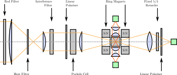
Figure 1: Schematic of a typical modern BiSON resonance scattering spectrophotometer. Light travels from left to right. The green boxes indicate detector locations. The magnetic field across the vapour cell is longitudinal, with the field axis aligned with the optical axis.

The original BiSON resonance scattering spectrophotometer (RSS) developed for Doppler velocity astronomical observations is described by Brookes et al. [10]. Modern BiSON RSS follow the same principles but make use of slightly different designs, and a typical example is shown in Figure 1. Light from the Sun is first passed through a $30\text{\,}\mathrm{mm}$ diameter aperture, and a pair of lenses in a Keplerian telescope arrangement are used to compress the beam reducing the diameter in preparation for subsequent smaller optics. A red long-pass filter, and an infra-red short-pass filter, form a pair to relieve the thermal load on the instrumentation. An interference filter with a bandwidth of $1.5\text{\,}\mathrm{nm}$ is used to isolate only the potassium D1 Fraunhofer line at $769.898\text{\,}\mathrm{nm}$, excluding the D2 line. The potassium is contained within a small cubic glass cell with sides of length $17\text{\,}\mathrm{mm}$, and a short stem. The stem is typically heated to around $90\text{\,}\mathrm{\SIUnitSymbolCelsius}$ to cause the formation of potassium vapour within the cell, with the cubic cell itself maintained at a temperature higher than this to ensure the glass remains clear of solid potassium. The cell is placed in a longitudinal magnetic field which causes the absorption line to be Zeeman split into two components, where their separation is dependent on the magnetic field strength. Splitting the lab reference-frame in this way allows measurements to be taken at two working points on the corresponding absorption line in the solar atmosphere. The polarisation component is selected using a linear polariser and an electro-optic Pockels-effect quarter-wave retarder. The polarisation is switched at approximately $100\text{\,}\mathrm{Hz}$ and a normalised ratio, R, formed,

$$R=\frac{I_{\mathrm{b}}-I_{\mathrm{r}}}{I_{\mathrm{b}}+I_{\mathrm{r}}}~{},$$ (1)

where $I_{\mathrm{b}}$ and $I_{\mathrm{r}}$ are the measured intensities in the blue and red wings respectively. Normalising the ratio in this way reduces the effect of atmospheric scintillation allowing low-noise photometry through Earth’s atmosphere [11], and also means it is unnecessary to know the precise value of the magnetic field strength or the precise frequency of the potassium line on the Sun. Light is focused into the centre of the potassium cell, where it is resonantly scattered by the vapour. Light that interacts with the vapour is scattered isotropically, and it is this isotropic nature that is leveraged by the BiSON resonance scattering spectrophotometers to move a photon away from the instrumental optical axis and into a detector. Two photodiode detectors on either side of the beam return a precise measurement of the changing solar radial velocity. A third detector monitors unscattered light that passes directly through the instrument.

There are several natural broadening processes which affect the properties of an absorption line, and it is necessary to understand the environmental factors (temperature and pressure) that affect these processes when building a model of expected instrumentation performance and informing new designs [8].

3 Resonance Radiation

3.1 Natural Line Width

In a gas that forms an absorption line, the absorption coefficient $\kappa_{\nu}$ of the gas is defined in terms of,

$$I_{\nu}=I_{0}e^{-\kappa_{\nu}x}~{},$$ (2)

where $I_{0}$ is the intensity of incident light, $I_{\nu}$ is the intensity of the transmitted light, and $x$ is the thickness of the absorbing material. The units of the absorption coefficient are always expressed in terms of the reciprocal of the units of $x$ such that the exponent becomes a unitless ratio.

It can be shown [12, p. 95] that the integral of $\kappa_{\nu}$ over all frequencies is equal to,

$$\int\kappa_{\nu}\mathrm{d}\nu=\frac{\lambda_{0}^{2}}{8\pi}\frac{g_{2}}{g_{1}}\frac{N}{\tau}\left(1-\frac{g_{1}}{g_{2}}\frac{N^{\prime}}{N}\right)~{},$$ (3)

where $\lambda_{0}$ is the wavelength at the centre of the absorption line, $\tau$ the lifetime of the excited state, and $g_{1}$ and $g_{2}$ are the statistical weights of the normal and excited states respectively. $N$ is the number density of atoms of which $[N-N^{\prime}]$ are capable of absorbing in the frequency range $\nu$ to $\nu~{}+~{}\mathrm{d}\nu$, and similarly $N^{\prime}$ is the number of excited atoms that are capable of emitting in this range. In the case where the ratio of excited atoms to normal atoms is very small ($\leqslant~{}10^{-4}$) then $N^{\prime}$ can be neglected and equation 3 reduces to,

$$\int\kappa_{\nu}\mathrm{d}\nu=\frac{\lambda_{0}^{2}}{8\pi}\frac{g_{2}}{g_{1}}\frac{N}{\tau}~{},$$ (4)

and this result shows that the integral of the absorption coefficient is constant if $N$ remains constant. This assumption can normally be made when the formation of excited atoms is due to absorption of a beam of light. Where a gas is electrically excited at high current densities, for example in a gas discharge lamp, the number of excited atoms may become a high fraction of the total number and so the simplification in equation 4 cannot be made. In the case where all atoms capable of absorbing at a certain frequency are already excited, the gas is said to be saturated and no further absorption can take place at that frequency.

Although the energy of an atomic transition is fixed, and therefore similarly the frequency of light with which it can interact, the absorption profile has a natural line width which arises from the uncertainty principle. When considered in the form,

$$\Delta E\Delta t>\frac{\hbar}{2}~{},$$ (5)

where $\Delta E$ is the energy, $\Delta t$ the lifetime, and $\hbar$ the reduced Planck constant, the result suggests that for extremely short excited state lifetimes there will be a significant uncertainty in the energy of the photon emitted. If the energy of many photons are measured the distribution formed is Lorentzian in shape, where $\Gamma$ is the width parameter for a Lorentzian profile. If we assume the lifetime in the excited state is the uncertainty in time (i.e., $\tau=\Delta t$) then,

$$\Delta E=\frac{\Gamma}{2}=\frac{\hbar}{2\tau}~{},$$ (6)

and so,

$$\Gamma=\frac{\hbar}{\tau}~{},$$ (7)

which shows that the natural line width is inversely proportional to the lifetime of the atom in the excited state. Mishra [13] observed the natural lifetime of the potassium $4^{2}P_{\frac{1}{2}}$ – $4^{2}S_{\frac{1}{2}}$ transition to be $27\text{\,}\mathrm{ns}$. Using equation 7 this corresponds to a Lorentzian width of $2.44\text{\times}{10}^{-8}\text{\,}\mathrm{eV}$. We can convert this to frequency using the relation $E=h\nu$, and so equation 6 becomes,

$$\Delta\nu=\frac{1}{4\pi\tau}~{},$$ (8)

producing a width of $5.9\text{\,}\mathrm{MHz}$. For the line centre of the $4^{2}P_{\frac{1}{2}}$ – $4^{2}S_{\frac{1}{2}}$ atomic transition at $769.898\text{\,}\mathrm{nm}$ this is a full width at half maximum (FWHM) of just $1.166\text{\times}{10}^{-05}\text{\,}\mathrm{nm}$, which is equivalent to a Doppler velocity of $4.54\text{\,}\mathrm{m}\text{\,}{\mathrm{s}}^{-1}$.

3.2 Pressure Broadening

Pressure acts to modify the natural line width. When an excited atom collides with another particle, it can be stimulated to decay earlier than would be the case for its natural lifetime. Continuing the argument from the uncertainty principle as before, if the lifetime is reduced than the uncertainty on the energy emitted must increase and hence broaden the line width. As the pressure increases, the likelihood of collisions increases.

Experimental conditions are usually selected to ensure that pressure broadening is minimised to a level of insignificance, and this is the case for our vapour reference cells which are placed under vacuum before being filled with their reference element. We will neglect this effect.

3.3 Doppler Broadening

Since the atoms in a gas are moving, the wavelength of light absorbed or emitted by the gas will be shifted according to the standard non-relativistic Doppler formula,

$$\frac{\Delta\lambda}{\lambda_{0}}=-\frac{\Delta\nu}{\nu_{0}}=\frac{v}{c}~{},$$ (9)

where $\Delta\lambda$ is the shifted wavelength, $\lambda_{0}$ is the rest wavelength, $v$ the speed, and $c$ the speed of light. Similarly, $\Delta\nu$ is the shift in frequency, and $\nu_{0}$ is the frequency at rest. The atoms in a gas are moving at speeds defined by the Maxwell-Boltzmann distribution, and so a spectral line will be broadened into a range of possible wavelengths with a Gaussian distribution. The FWHM due to Doppler broadening is given by,

$$\Delta\nu=\sqrt{\frac{8k_{\mathrm{B}}T\ln{2}}{mc^{2}}}\nu_{0}$$ (10)

which can be used to calculate the expected Doppler width of the absorption line. Potassium has a standard atomic weight of $39.0983\text{\,}\mathrm{u}$. For a reference vapour at $100\text{\,}\mathrm{\SIUnitSymbolCelsius}$ the broadening is $0.0017\text{\,}\mathrm{nm}$. This is equivalent to a Doppler velocity of $663\text{\,}\mathrm{m}\text{\,}{\mathrm{s}}^{-1}$, almost 150 times larger than the width produced by natural broadening. On the Sun at a temperature of $5777\text{\,}\mathrm{K}$, the D1 line width due to Doppler broadening is $0.0067\text{\,}\mathrm{nm}$.

It may be shown [12, p. 99] that when considering only Doppler broadening, the absorption coefficient of a gas is given by,

$$\kappa_{\nu}=\kappa_{0}e^{-\left[\frac{2(\nu-\nu_{0})}{\Delta\nu}\sqrt{\ln{2}}\right]^{2}}~{},$$ (11)

where $\kappa_{0}$ is the ideal maximum absorption for Doppler broadening alone, and $\Delta\nu$ is the Doppler breadth defined in equation 10. The integral of $\kappa_{\nu}$ over all frequencies is equal to,

$$\int\kappa_{\nu}\mathrm{d}\nu=\frac{1}{2}\sqrt{\frac{\pi}{\ln{2}}}\kappa_{0}\Delta\nu~{},$$ (12)

and this depends only on the temperature and the atomic mass of the atoms forming the vapour, which for a given material means temperature is the only variable.

4 Vapour Optical Depth

To be able to interpret the results of any experiments involving a gas reference cell, we need a mathematical expression for the absorption of the gas under the combined broadening conditions. We know that no matter what physical processes are responsible for the formation of a spectral line, the integral of the absorption coefficient over all frequencies must remain constant if the number of atoms remains constant. This can be explained more simply by considering that any given atom can have the appropriate physical properties (i.e., speed, direction) to interact with only one particular frequency. If a spectral line is broadened, then the absorption depth must simultaneously reduce due to there being fewer atoms available to interact at the line centre. From this we can equate equations 4 and 12 thus,

$$\frac{\lambda_{0}^{2}}{8\pi}\frac{g_{2}}{g_{1}}\frac{N}{\tau}=\frac{1}{2}\sqrt{\frac{\pi}{\ln{2}}}\kappa_{0}\Delta\nu~{},$$ (13)

and solving for $\kappa_{0}$ produces [12, p. 100],

$$\kappa_{0}=\frac{2}{\Delta\nu}\sqrt{\frac{\ln{2}}{\pi}}\frac{\lambda^{2}_{0}}{8\pi}\frac{g_{2}}{g_{1}}\frac{N}{\tau}~{},$$ (14)

which is the maximum absorption possible. This can be combined with the expected line profile to produce the final value for $\kappa_{\nu}$. We have already seen such an example in equation 11 where for a line profile dominated by Doppler broadening $\kappa_{\nu}$ has a Gaussian profile.

The absorption coefficient and thickness in equation 2 can be combined into one term $\tau_{\nu}$, known as the optical depth,

$$I_{\nu}=I_{0}e^{-\tau_{\nu}}~{},$$ (15)

where, as before, $I_{0}$ is the intensity of incident light, and $I_{\nu}$ is the intensity of the transmitted light. Unit optical depth is therefore defined as the optical thickness that reduces the photon flux by a factor of $1/e$. It should be noted that $\tau_{\nu}$ is specifically a different quantity from $\tau$ the lifetime of the excited state.

We know that the $769.898\text{\,}\mathrm{nm}$ line profile formed by potassium vapour is dominated by Doppler broadening, and so equation 11 is valid to describe the distribution. In order to evaluate $\kappa_{\nu}$ we need to know the value of all the terms in equation 14 – temperature $T$, the atomic mass $m$, the frequency and wavelength of the line centre $\nu_{0}$ and $\lambda_{0}$, the number density of absorbing atoms $N$, the lifetime of the excited state $\tau$, and the degeneracy of the $4^{2}P_{\frac{1}{2}}$ – $4^{2}S_{\frac{1}{2}}$ energy levels $g_{1}$ and $g_{2}$, respectively.

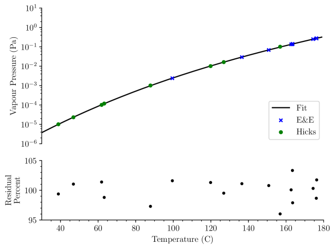
Figure 2: Upper: The blue crosses and green dots show measurements of the vapour pressure of potassium made independently by Edmondson and Egerton [14] and Hicks [15] at various temperatures. The black line shows a cubic fit to the data. Lower: The residuals to the fit in terms of percentage (i.e., $100\cdot(\textrm{model}/\textrm{data})$). The uncertainty on the source data are not available, and so no error bars are plotted.

We already know the lifetime $\tau$ to be $27\text{\,}\mathrm{ns}$, the atomic mass to be $39.0983\text{\,}\mathrm{u}$, the central wavelength to be $769.898\text{\,}\mathrm{nm}$, and it may be shown [12, p. 97] that the ratio $g_{2}/g_{1}$ is unity. The temperature of the reference cell is controlled, and so the only remaining term is the number density. We can determine the number density based on the vapour pressure, since as we saw earlier it depends only on the temperature and not on the amount of physical material.

The vapour in a gas reference cell can be treated as an ideal gas since the pressure is by design very low. The cells are evacuated and baked out before being filled with a small amount of potassium. Since the pressure is low, there will be few interactions between particles. The ideal gas law is defined as,

$$pV=Nk_{\mathrm{B}}T~{},$$ (16)

where $p$ is the pressure, $V$ the volume, $N$ the number of atoms or molecules, $k_{\mathrm{B}}$ the Boltzmann constant, and $T$ the temperature. If we combine the number of atoms and the volume into one parameter to form the number density $n(T)$, and define the pressure in terms of temperature then equation 16 simplifies to,

$$n(T)=\frac{p(T)}{k_{\mathrm{B}}T}~{},$$ (17)

which depends only on the vapour pressure and the temperature.

Previous independent measurements have been made [14, 15] of the vapour pressure of potassium at various temperatures. These data have been used to fit a polynomial in log space,

$$p_{\mathrm{vapour}}=e^{a\,T^{3}+b\,T^{2}+c\,T+d}~{},$$ (18)

where $p_{\mathrm{vapour}}$ is the vapour pressure and $T$ is the temperature in Kelvin. The values of the four fit coefficients are shown in Table 1. A plot of results from this model against the original data are shown in Figure 2. The model residuals are all within $\pm 5\text{\,}\mathrm{\char 37\relax}$ of the original value, with an upper limit to the fit of $449\text{\,}\mathrm{K}$ ($175\text{\,}\mathrm{\SIUnitSymbolCelsius}$). For a typical vapour temperature of $100\text{\,}\mathrm{\SIUnitSymbolCelsius}$ the number density required is $4.9\text{\times}{10}^{17}\text{\,}{\mathrm{m}}^{-3}$. This is equivalent to $3.2\text{\times}{10}^{-8}\text{\,}\mathrm{kg}$ of potassium – if you can see solid potassium in the cell then there is enough to form the required vapour.

Table 1: Potassium vapour pressure model coefficients.

Coefficient	Value	Uncertainty
a	$6.005\,421\,123\,5\text{\times}{10}^{-07}$	$8.746\,869\,416\,7\text{\times}{10}^{-08}$
b	$-8.912\,131\,894\,2\text{\times}{10}^{-04}$	$1.007\,298\,376\,8\text{\times}{10}^{-04}$
c	$4.889\,749\,974\,5\text{\times}{10}^{-01}$	$3.839\,917\,119\,5\text{\times}{10}^{-02}$
d	$-9.555\,120\,408\,0\text{\times}{10}^{01}$	$4.843\,625\,849\,5\text{\times}{10}^{00}$

We now have everything in place to be able to calculate the optical depth of a potassium vapour from equation 15. We know all of the parameters required to calculate the absorption coefficient $\kappa_{0}$ in equation 14 by determining the vapour pressure from equation 18, and we can calculate the wavelength-dependent absorption coefficient from equation 11. The model was verified by probing a potassium vapour cell using a tunable diode laser.

5 Laser Calibration

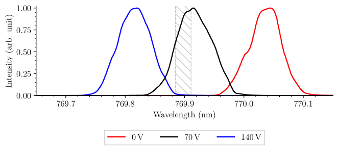
Figure 3: Toptica DLC pro tunable diode laser profile tuning range, measured using an Agilent 86142B optical spectrum analyser. The line width is much narrower than indicated in the figure. The measured FWHM is broadened to the minimum $0.06\text{\,}\mathrm{nm}$ resolution bandwidth of the spectrum analyser. The red and blue lines indicate the extent of the voltage-controlled piezo fine-tuning range after prior coarse tuning to approximately $769.9\text{\,}\mathrm{nm}$. The hatched area indicates the extent of our wavelength region of interest.

We used a Toptica DLC pro tunable diode laser, which is a Littrow-style external cavity diode laser (EDCL) [16]. The installed laser diode has an emission spectrum and tuning range of $765\text{\,}\mathrm{nm}805\text{\,}\mathrm{nm}$. The primary tuning mechanism is by altering the angle of incidence of the grating forming the external cavity, which for coarse adjustment is done using a micrometer screw, and for fine adjustment by varying the applied voltage to a piezo actuator. Tuning can also be achieved by changing the diode drive current and temperature. The diode suffers mode-hopping as the tuning parameters are adjusted, but this can be mitigated by varying all parameters simultaneously. The typical mode-hop-free tuning-range (MHFTR) is quoted at $20\text{\,}\mathrm{GHz}50\text{\,}\mathrm{GHz}$, which at a wavelength of $770\text{\,}\mathrm{nm}$ is equivalent to $40\text{\,}\mathrm{pm}98\text{\,}\mathrm{pm}$. Achieving this range can be tricky due to the interaction of all the various tuning methods. The typical line width achieved by a Littrow-style ECDL over a duration of $5\text{\,}\mathrm{\SIUnitSymbolMicro s}$ is $10\text{\,}\mathrm{kHz}300\text{\,}\mathrm{kHz}$, which again at a wavelength of $770\text{\,}\mathrm{nm}$ is less than $0.6\text{\,}\mathrm{fm}$. The main contributions to the line width are electronic noise, acoustic noise, and other vibrations that affect the cavity length.

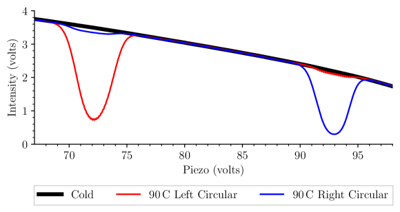
Figure 4: Laser intensity flat-field calibration.

The output of the ECDL has no intrinsic wavelength calibration, except that the wavelength must be somewhere within the broadband output of the model of installed laser diode. In order to coarse-tune the laser to approximately $769.9\text{\,}\mathrm{nm}$ the output wavelength was measured using an Agilent 86142B optical spectrum analyser [17], shown in Figure 3. The 86142B has a resolution bandwidth (RBW) of $0.06\text{\,}\mathrm{nm}$ and so the measured laser line width is considerably broadened. This resolution is sufficient to allow use of the coarse manual micrometer screw adjustment to ensure the required wavelength is positioned within the narrow scan range of the piezo actuator. The resolution is insufficient to tune the wavelength precisely to the desired absorption line, but once coarse calibration is achieved simply scanning between the piezo limits allows the absorption line to be found. In order to calibrate the width and depth of the absorption line at varying temperature, it is necessary to calibrate the piezo voltage in terms of wavelength and to normalise the beam intensity. This calibration is non-trivial and we will now go on to discuss the steps required to achieve the final overall calibration.

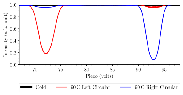
Figure 5: Piezo voltage calibration after flat-field adjustment. The line centres occur at $72.2\text{\,}\mathrm{V}$ and $92.9\text{\,}\mathrm{V}$. The different depths are due to slight misalignment of the polarising filters. There is also some evidence of non-linearity in the wavelength scan observed from slight differences in the profile widths.

Since BiSON spectrophotometers use a magnetic field to Zeeman split the reference absorption line and produce two separate instrumental passbands, this technique can be used to produce a known wavelength separation and so calibrate the piezo. Figure 4 shows the two components of the Zeeman split absorption line with the cell heated to $90\text{\,}\mathrm{\SIUnitSymbolCelsius}$ in a $0.3\text{\,}\mathrm{T}$ longitudinal magnetic field. The beam intensity is not uniform across the piezo scan due to a drive-current feed-forward mechanism employed to increase the MHFTR of the diode laser. It is imperative that the diode does not mode-hop during the scan since this would result in different wavelength calibrations either side of the mode-hop, destroying the overall calibration. The feed-forward adjusts the drive-current proportionally with the piezo position-voltage by a factor of $-0.32\text{\,}\mathrm{mA}\text{\,}{\mathrm{V}}^{-1}$, which helps prevent mode-hopping but has the undesired side-effect of changing the beam intensity. If a mode-hop continues to appear at an inconvenient wavelength, then the temperature of the diode can be adjusted to move the mode-hop elsewhere. The mean drive-current and detector-gain has to be selected carefully to ensure that the current always stays above the lasing threshold of $109\text{\,}\mathrm{mA}$, but also that the beam intensity does not exceed the dynamic range of the detector throughout the whole piezo scan range. Once a mode-hop-free scan has been achieved with a beam intensity that is comfortably within the dynamic range of the detector, a flat-field can be captured and used to normalise the intensity of the scan, shown in Figure 5.

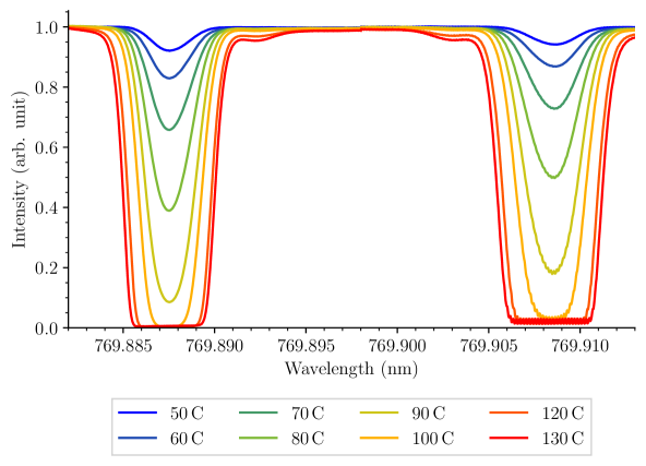
Figure 6: Vapour cell absorption intensity profiles at a range of temperatures.

We can complete the calibration by making use of the known position of the two Zeeman components, and applying the splitting to the piezo voltages at the measured line centres. The calibrated absorption profiles for eight different cell temperatures are shown in Figure 6. There is some evidence of slight misalignment of the polarising filters indicated by differences in absorption depth between the two polarisation states. There is also some non-linearity in the wavelength scan indicated by a slight difference in width between the two polarisation states. These errors are small and will be mitigated against by fitting the model to both absorption components simultaneously, allowing all equal-and-opposite errors to cancel.

6 Model Validation

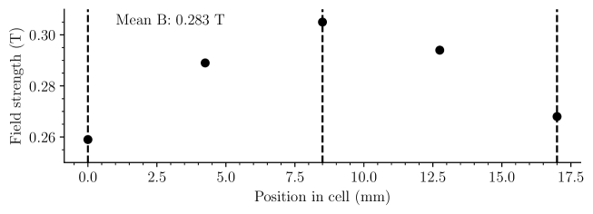
Figure 7: On-axis magnetic variation inside the cell oven. The field inhomogeneity adds an additional source of spectral broadening which must be included in the model.

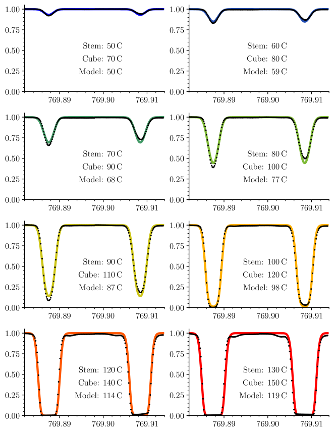
Figure 8: Modelled absorption profiles at a range of vapour temperatures. The dotted lines show the measured absorption profile. The solid lines show the results of the fit to the data. Both absorption components are fitted simultaneously allowing systematic equal-and-opposite errors to cancel.

Table 2: Fitted model parameters at a range of vapour temperatures.

Oven Temp		Model Temp			Broadening Factor
Stem	Cube	Stem	Uncertainty	$\Delta T$	Scale	Uncertainty
$50$	$70$	$49.938\,016\,835\,294\,83$	$0.059\,113\,852\,741\,602\,47$	$-0.061\,983\,164\,705\,168\,29$	$1.549\,797\,751\,690\,003\,4$	$0.010\,225\,235\,529\,756\,882$
$60$	$80$	$59.071\,934\,404\,884\,54$	$0.058\,066\,785\,163\,415\,24$	$-0.928\,065\,595\,115\,462\,8$	$1.593\,463\,750\,618\,715$	$0.009\,660\,575\,562\,317\,709$
$70$	$90$	$67.876\,399\,513\,686\,6$	$0.053\,875\,034\,984\,575\,59$	$-2.123\,600\,486\,313\,407$	$1.551\,258\,089\,828\,436$	$0.008\,040\,919\,986\,667\,729$
$80$	$100$	$76.785\,135\,352\,922\,92$	$0.049\,740\,470\,851\,325\,234$	$-3.214\,864\,647\,077\,078\,5$	$1.476\,174\,247\,567\,248\,1$	$0.006\,132\,750\,128\,753\,006$
$90$	$110$	$87.326\,606\,201\,860\,5$	$0.060\,185\,612\,987\,991\,16$	$-2.673\,393\,798\,139\,5$	$1.395\,458\,493\,606\,643\,4$	$0.004\,645\,848\,115\,386\,062$
$100$	$120$	$97.802\,526\,968\,519\,91$	$0.143\,756\,306\,036\,066\,84$	$-2.197\,473\,031\,480\,086\,5$	$1.361\,130\,316\,319\,705\,7$	$0.005\,682\,520\,990\,971\,153$
$120$	$140$	$114.124\,859\,744\,293\,99$	$0.605\,734\,316\,440\,814$	$-5.875\,140\,255\,706\,015$	$1.412\,580\,319\,424\,884\,7$	$0.013\,110\,165\,784\,624\,19$
$130$	$150$	$119.236\,331\,888\,108\,75$	$0.846\,026\,865\,907\,446\,2$	$-10.763\,668\,111\,891\,25$	$1.469\,473\,328\,711\,452\,3$	$0.016\,709\,308\,941\,953\,73$

The laser calibration is dependent on the accuracy and uniformity of the vapour cell longitudinal magnetic field. The field strength at several points inside the cell oven was measured using a Hirst GM04 Gaussmeter, which is factory calibrated using nuclear magnetic resonance to correct for irregularities in the supplied semi-flexible transverse Hall probe. It was found that the target field strength of $0.3\text{\,}\mathrm{T}$ is achieved only at the cell centre and drops to approximately $0.26\text{\,}\mathrm{T}$ at the front and rear of the cell oven, as shown in Figure 7. The mean field strength is $0.283\text{\,}\mathrm{T}$. Due to the variation in field strength, it is not necessary to measure the field strength to high precision, however this does mean that the absorption profile will have an additional broadening factor caused by the non-uniform magnetic field, and the FWHM determined from equation 10 has to be modified to allow an additional degree of freedom.

The resulting final model has been fitted against absorption profiles for all eight vapour temperatures in Figure 6. Both absorption components are fitted simultaneously allowing systematic equal-and-opposite errors to cancel. The results are shown in Figure 8, where the dotted lines show the measured absorption profile and the solid lines show the results of the fit to the data. The fitted parameters and uncertainties listed in Table 2.

All fitted temperatures indicate that the vapour pressure is controlled by the temperature of the solid potassium in the stem of the cell. The temperature of the upper cube of the cell simply has to be higher than the stem and high enough to ensure that deposition of solid potassium onto the windows does not occur. The increasing difference between the model temperature and the stem temperature at higher values is an indication of the difficulties of coupling heat efficiently into the cell. Heating of the stem is achieved by a foil heating element wrapped around the glass, and heat does of course leak into the surrounding chassis as well as heating the cell. At higher temperatures the losses become more significant and it becomes progressively more difficult to effectively heat the cell, and this is indicated by the real temperature of the vapour as determined from the model being a few degrees below the measured temperature of the stem heating element.

7 Instrumentation Parameters

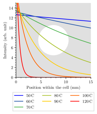
Figure 9: Absorption through a typical $15\text{\,}\mathrm{mm}$ BiSON vapour cell at various temperatures. The absorption coefficient is modelled as monochromatic but with the initial intensity scaled by the expected FWHM to compensate for the differences in spectral bandwidth. The white circle in the centre indicates the typical $6\text{\,}\mathrm{mm}$ aperture of a scattering detector.

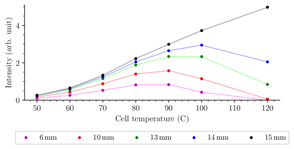
Figure 10: Optimum vapour temperature for maximum scattering intensity at a range of aperture sizes.

The model can be used to estimate the scattering performance of the cell and the effect of different detector aperture sizes and positions. Figure 9 shows the expected intensity change as light passes through the cell determined from equation 2. The absorption coefficient is modelled as monochromatic from equation 14 but with the initial intensity scaled by the expected FWHM to compensate for the differences in spectral bandwidth. We make an assumption that any photon is scattered only once. Any secondary (or further multiple) scattering of light that has been moved away from the optical axis in the direction of a scattering detector will be isotropic. The detected intensity will be reduced by the optical depth between the point of scattering within the cell and the detector, and so it is important when calculating the total expected throughput, but has only a minor effect when considering variations in aperture size. The white circle in the centre of the figure indicates the typical $6\text{\,}\mathrm{mm}$ aperture of a scattering detector, with scattered light perpendicular to the page coming out towards the reader as the beam passes through from left to right. It is clear that at low temperatures there is very little scattered light due to the small absorption coefficient. At high temperatures almost all the light is scattered at the front of the cell and so not captured by the detector. This implies that there will be some optimum temperature at which the measured scattering intensity is greatest. By considering the change in intensity within the area of the white circle, we can estimate the intensity of light scattered away from the beam optical axis. Figure 10 shows the estimated scattering intensity for several aperture sizes and vapour temperatures. If the aperture is equal to the size of the vapour cell then all the light scattered towards the detector is captured, and the intensity continually increases with temperature. As the aperture size is reduced a temperature plateau forms. One might expect that the ideal aperture is as large as possible in order to maximise the intensity of scattered light and so maximise the signal-to-noise ratio. However, there are several reasons why this is not the case. Applying a smaller aperture and causing the temperature plateau to form minimises the effect of fluctuations in vapour temperature, and the temperature-width of the plateau is greatest at smaller apertures. Also, it is imperative to eliminate non-resonantly scattered light from reaching the detector, such as specular reflections from the cell glass especially at the edges and corners of the cell, and again this is best achieved via small apertures effectively acting as a baffle.

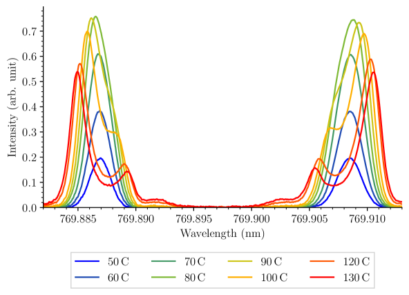
Figure 11: Vapour cell scattering intensity profiles at a range of temperatures. The profile asymmetry seen at temperatures above the ideal temperature is a result of the inhomogeneity of the magnetic field.

The scattering detectors used in most BiSON instrumentation employ $6\text{\,}\mathrm{mm}10\text{\,}\mathrm{mm}$ circular apertures which suggests that the maximum intensity will be found at a stem temperature of approximately $80\text{\,}\mathrm{\SIUnitSymbolCelsius}90\text{\,}\mathrm{\SIUnitSymbolCelsius}$. Many BiSON instruments run at a stem temperature of $90\text{\,}\mathrm{\SIUnitSymbolCelsius}$ and a cube temperature of $110\text{\,}\mathrm{\SIUnitSymbolCelsius}$ and so these results agree with expectation based on experience. At this temperature the optical depth is approximately one if measured from the front of the cell to the centre, or approximately two from the front of the cell to the rear.

Figure 11 shows the scattering profiles taken simultaneously with the absorption profiles shown in Figure 6 over a range of vapour cell temperatures, and the intensity peaks at approximately $80\text{\,}\mathrm{\SIUnitSymbolCelsius}90\text{\,}\mathrm{\SIUnitSymbolCelsius}$ as expected. The profile asymmetry seen at high temperatures is a result of the inhomogeneity of the magnetic field. At lower temperatures, light is detected from across the whole aperture, and the peaks are centred at the wavelengths corresponding to the splitting produced by the mean field strength. At higher temperatures, the scattering is dominated towards the front of the cell within the weaker part of the field, and not seen by the detector. The detector captures only the remaining small fraction of light at the wavelength corresponding to the higher field strength at the centre of the cell, leading to the observed offset weighted towards higher field strength.

8 Conclusion

We have developed a model of a BiSON potassium vapour cell and validated the output of the model using a tunable diode laser, where the model was found to effectively reproduce the properties of the cell. Previously the ideal temperature working point was determined empirically, and the result found here now puts the choice on a firm footing.

The model can be used to assess vapour cells of different size and shape, and determine the ideal operating vapour temperature and configuration of detectors, allowing comparison of expected performance between existing BiSON vapour cells and commercially available alternatives. Previously the optical depth of the cell, and the location within the cell where most of the scattering occurs, has not been known precisely. This information is essential when designing new instrumentation, such as the prototype next generation of BiSON spectrophotometers (BiSON:NG [8]), where the aim is to make use of off-the-shelf components to simplify and miniaturise the instrumentation as much as practical.

9 Open Data

All code and data are freely available for download from the University of Birmingham eData archive [18], and also from the source GitLab repository [19].

References

- Svanberg et al. [1979] S. Svanberg, Amyand David Buckingham, George William Series, Edward Roy Pike, and J. G. Powles. Atomic spectroscopy by resonance scattering. Philosophical Transactions of the Royal Society of London. Series A, Mathematical and Physical Sciences, 293(1402):215–222, 1979. doi: 10.1098/rsta.1979.0091. URL https://royalsocietypublishing.org/doi/abs/10.1098/rsta.1979.0091.
- Preston [1996] Daryl W. Preston. Doppler-free saturated absorption: Laser spectroscopy. American Journal of Physics, 64(11):1432–1436, 1996. doi: 10.1119/1.18457. URL https://doi.org/10.1119/1.18457.
- Svanberg [2004] Sune Svanberg. Laser Spectroscopy, pages 287–387. Springer Berlin Heidelberg, Berlin, Heidelberg, 2004. ISBN 978-3-642-18520-5. doi: 10.1007/978-3-642-18520-5˙9. URL https://doi.org/10.1007/978-3-642-18520-5_9.
- Svanberg et al. [2016] Sune Svanberg, Guangyu Zhao, Hao Zhang, Jing Huang, Ming Lian, Tianqi Li, Shiming Zhu, Yiyun Li, Zheng Duan, Huiying Lin, and Katarina Svanberg. Laser spectroscopy applied to environmental, ecological, food safety, and biomedical research. Opt. Express, 24(6):A515–A527, Mar 2016. doi: 10.1364/OE.24.00A515. URL http://www.opticsexpress.org/abstract.cfm?URI=oe-24-6-A515.
- Grundahl et al. [2017] F. Grundahl, M. Fredslund Andersen, J. Christensen-Dalsgaard, V. Antoci, H. Kjeldsen, R. Handberg, G. Houdek, T. R. Bedding, P. L. Pallé, J. Jessen-Hansen, V. Silva Aguirre, T. R. White, S. Frandsen, S. Albrecht, M. I. Andersen, T. Arentoft, K. Brogaard, W. J. Chaplin, K. Harpsøe, U. G. Jørgensen, I. Karovicova, C. Karoff, P. Kjærgaard Rasmussen, M. N. Lund, M. Sloth Lundkvist, J. Skottfelt, A. Norup Sørensen, R. Tronsgaard, and E. Weiss. First Results from the Hertzsprung SONG Telescope: Asteroseismology of the G5 Subgiant Star Herculis. The Astrophysical Journal, 836(1):142, feb 2017. doi: 10.3847/1538-4357/836/1/142. URL https://doi.org/10.3847%2F1538-4357%2F836%2F1%2F142.
- Seemann et al. [2014] U. Seemann, G. Anglada-Escude, D. Baade, P. Bristow, R. J. Dorn, R. Follert, D. Gojak, J. Grunhut, A. P. Hatzes, U. Heiter, D. J. Ives, P. Jeep, Y. Jung, H.-U. Käufl, F. Kerber, B. Klein, J.-L. Lizon, M. Lockhart, T. Löwinger, T. Marquart, E. Oliva, J. Paufique, N. Piskunov, Eszter Pozna, A. Reiners, A. Smette, J. Smoker, E. Stempels, and E. Valenti. Wavelength calibration from 1–5 m for the CRIRES+ high-resolution spectrograph at the VLT. In Suzanne K. Ramsay, Ian S. McLean, and Hideki Takami, editors, Ground-based and Airborne Instrumentation for Astronomy V, volume 9147, pages 1771 – 1783. International Society for Optics and Photonics, SPIE, 2014. doi: 10.1117/12.2056668. URL https://doi.org/10.1117/12.2056668.
- Hale et al. [2016] S. J. Hale, R. Howe, W. J. Chaplin, G. R. Davies, and Y. P. Elsworth. Performance of the Birmingham Solar-Oscillations Network (BiSON). Sol. Phys., 291(1):1–28, January 2016. ISSN 1573-093X. doi: 10.1007/s11207-015-0810-0. URL https://doi.org/10.1007/s11207-015-0810-0.
- Hale [2019] S. J Hale. Birmingham Solar Oscillations Network: The Next Generation. PhD thesis, School of Physics and Astronomy, University of Birmingham, UK, July 2019. URL https://etheses.bham.ac.uk/id/eprint/9010/.
- Boumier and Dame [1993] P. Boumier and L. Dame. Golf: A resonance spectrometer for the observation of solar oscillations I) Numerical model of the sodium cell response. Experimental Astronomy, 4(2):87–104, Jun 1993. doi: 10.1007/BF01588347.
- Brookes et al. [1978] J. R. Brookes, G. R. Isaak, and H. B. van der Raay. A resonant-scattering solar spectrometer. MNRAS, 185:1–18, October 1978. doi: 10.1093/mnras/185.1.1. URL http://adsabs.harvard.edu/abs/1978MNRAS.185....1B.
- Hale et al. [2020] S. J. Hale, W. J. Chaplin, G. R. Davies, Y. P. Elsworth, R. Howe, and P. L. Pallé. Measurement of Atmospheric Scintillation during a Period of Saharan Dust (Calima) at Observatorio del Teide, Iz̃ana, Tenerife, and the Impact on Photometric Exposure Times. PASP, 132(1009):034501, Mar 2020. doi: 10.1088/1538-3873/ab6753. URL http://doi.org/10.1088/1538-3873/ab6753.
- Mitchell and Zemansky [1961] A.C.G. Mitchell and M.W. Zemansky. Resonance Radiation and Excited Atoms. The Cambridge series of physical chemistry. University Press, 1961. URL https://books.google.co.uk/books?id=Ic7vAAAAMAAJ.
- Mishra [1950] B. Mishra. Lifetimes of mercury and potassium atoms in excited states. Phys. Rev., 77:153–153, January 1950. doi: 10.1103/PhysRev.77.153. URL http://link.aps.org/doi/10.1103/PhysRev.77.153.
- Edmondson and Egerton [1927] W. Edmondson and A. Egerton. The vapour pressures and melting points of sodium and potassium. Proceedings of the Royal Society of London A: Mathematical, Physical and Engineering Sciences, 113(765):520–533, 1927. ISSN 0950-1207. doi: 10.1098/rspa.1927.0005.
- Hicks [1963] W. T. Hicks. Evaluation of vapor-pressure data for mercury, lithium, sodium, and potassium. The Journal of Chemical Physics, 38(8):1873–1880, 1963. doi: 10.1063/1.1733889. URL http://scitation.aip.org/content/aip/journal/jcp/38/8/10.1063/1.1733889.
- Toptica [2017] Toptica. Tunable diode lasers. Datasheet BR-199-68A, Toptica Photonics AG, Lochhamer Schlag 19, D-82166 Graefelfing, Munich, Germany, January 2017. URL https://www.toptica.com/fileadmin/Editors_English/11_brochures_datasheets/01_brochures/toptica_BR_Scientific_Lasers.pdf.
- Agilent [2012] Agilent. Agilent 86142b optical spectrum analyzer technical overview. Datasheet 5980-0177E, Agilent Technologies Deutschland GmbH, Herrenberger Str. 130, 71034 Böblingen, Germany, January 2012. URL http://literature.cdn.keysight.com/litweb/pdf/5980-0177E.pdf?id=1627506.
- Hale [2020a] S. J Hale. Modelling the response of potassium vapour in resonance scattering spectroscopy, January 2020a. URL https://edata.bham.ac.uk/417/.
- Hale [2020b] S. J Hale. Modelling the response of potassium vapour in resonance scattering spectroscopy, January 2020b. URL https://gitlab.com/drstevenhale/vapour-resonance/-/tags/v1.0.