Nonlinear PCA for Spatio-Temporal Analysis of Earth Observation Data

Abstract

Remote sensing observations, products and simulations are fundamental sources of information to monitor our planet and its climate variability. Uncovering the main modes of spatial and temporal variability in Earth data is essential to analyze and understand the underlying physical dynamics and processes driving the Earth System. Dimensionality reduction methods can work with spatio-temporal datasets and decompose the information efficiently. Principal Component Analysis (PCA), also known as Empirical Orthogonal Functions (EOF) in geophysics, has been traditionally used to analyze climatic data. However, when nonlinear feature relations are present, PCA/EOF fails. In this work, we propose a nonlinear PCA method to deal with spatio-temporal Earth System data. The proposed method, called Rotated Complex Kernel PCA (ROCK-PCA for short), works in reproducing kernel Hilbert spaces to account for nonlinear processes, operates in the complex kernel domain to account for both space and time features, and adds an extra rotation for improved flexibility. The result is an explicitly resolved spatio-temporal decomposition of the Earth data cube. The method is unsupervised and computationally very efficient. We illustrate its ability to uncover spatio-temporal patterns using synthetic experiments and real data. Results of the decomposition of three essential climate variables are shown: satellite-based global Gross Primary Productivity (GPP) and Soil Moisture (SM), and reanalysis Sea Surface Temperature (SST) data. The ROCK-PCA method allows identifying their annual and seasonal oscillations, as well as their non-seasonal trends and spatial variability patterns. The main modes of variability of GPP and SM match expected distributions of land-cover and eco-hydrological zones, respectively; the inter-annual component of SM is shown to be highly correlated with El Niño Southern Oscillation (ENSO) phenomenon; and the SST annual oscillation is perfectly uncoupled in magnitude and phase from the global warming trend and ENSO anomalies, as well as from their mutual interactions. We provide a working source code of the presented method for the interested reader in https://github.com/DiegoBueso/ROCK-PCA.

I Introduction

In the last few decades, we have witnessed an ever growing availability of Earth system data: along with improved remote sensing observational data, a plethora of products, climate simulations and reanalysis data are now widely available. Yet, data does not necessarily mean information, and thus extracting the most important components (features) of the data is an urgent need, as well as a matter of very active research. Earth observation data is often described in both space and time (i.e. data cubes), and extracting their spatio-temporal components and patterns is one of the main goals in the geoscience and climate science communities. Such patterns are essential to analyze and understand the underlying physical dynamics and processes driving the Earth system [1, 2].

Natural processes, however, are usually masked by complex spatio-temporal feature relations, which makes the problem of identifying modes of variability specially challenging. The challenge is to derive spatial and temporal components that summarize the information content of the data cubes, while being physically meaningful and interpretable. Traditional techniques of feature extraction, such as the removal of mean seasonality, temporal trends, parametric fitting or harmonic decomposition are practical and commonly used [3, 4, 5, 6, 7]. However, they require prior knowledge and assumptions, and therefore impose expected relations that could not necessarily be found in data. This is probably the main reason why data driven decomposition methods have been largely adopted in geosciences and climate science in the last decades [8, 9, 10, 11, 12, 13, 14, 15].

Machine learning in general and dimensionality reduction in particular may help in extracting spatial and temporal components automatically. Dimensionality reduction methods can generally deal with data cubes and find the main features (components) efficiently. The application of such methods may help in uncovering relevant spatial patterns and dynamics of the underlying physics governing the Earth system. These techniques are also very useful to summarize (compress) the data into a reduced set of informative components. The analysis of the extracted components can shed light in the understanding of the Earth system because the intrinsic components may reveal correlations with known physical processes. Indeed, dimensionality reduction is widely used in the analysis of climate dynamics and teleconnections, and it is a key first step in observational causal discovery [13, 18].

Principal Component Analysis (PCA), also known in geophysics as Empirical Orthogonal Functions (EOFs), is widely used to obtain compact representations of the signal, and has been widely exploited to obtain spatio-temporal features in climatological studies [10, 9, 8]. Many extensions of PCA have been presented to deal with different specificities and applications in geophysics, including the extended EOF, the Multivariate EOF [4] or the Principal Oscillation patterns  [19] (see also a review in [20]). Interestingly, the Singular Spectrum Analysis (SSA) introduced the possibility of extracting spatial patterns at multiple time scales [21], but at the cost of introducing a delay parameter which makes the decomposition very sensitive to this parameter. A number of approaches not strictly related with EOF have also been proposed, such as the ones based on temporal domain periodicities and adaptations (e.g.  [22, 23]) or time-frequency transformations  [24, 25]. In recent years, machine learning decomposition approaches have emerged, mainly based on Gaussian Processes [26], Bayesian reconstruction [14], and on low-rank tensor learning  [27]. Most of these methods, however, assume orthogonality, periodicity, linearity or are not computationally affordable to deal with high dimensional problems. To deal with the spatio-temporal decomposition of Earth system data cubes, it is desirable that the methods i) are able to extract features which are potentially correlated –since real physical processes are usually coupled– , ii) are able to unveil the natural nonlinear relationships present in the data, and iii) do not assume any arbitrary parametric response function [28].

In this paper, we introduce a nonlinear PCA based on kernel methods [16] that addresses the main shortcomings found in the existing literature of spatio-temporal data decomposition. The proposed method, called Rotated Complex Kernel PCA (ROCK-PCA for short), has the following properties:

• Nonlinear. The method works in reproducing kernel Hilbert spaces to account for nonlinear processes [29]. Kernel methods have excelled in many problems in remote sensing, geosciences and climate sciences, mainly in classification and parameter retrieval, yet also for feature extraction and dimensionality reduction [17, 16, 30].

• Flexible. An extra rotation is included to improve the flexibility and physical interpretation of the decomposition. Typically, this has been addressed by means of the Varimax rotation [31]. Here we propose the Promax oblique method for improved versatility [32]. This rotation method alleviates the orthogonality constraint, and makes the principal components physically interpretable.

• Space and time decoupling. The method operates in the complex (kernel) domain to account for space and time features [33, 34, 10, 8]. The spatial and temporal modes are treated via the Hilbert transform [35], thus leading to spatial and temporally explicit eigendecompositions easy to analyze. Information about the amplitude and phase of the spatio-temporal features is extracted.

• Unsupervised. The criteria of maximum projection kurtosis is implemented as an automatic means to estimate a suitable value for the three parameters of our method i.e. the kernel hyperparameters, the specific rotation and the number of extracted components. The choice of maximum tailedness of the probability distributions was previously explored in feature extraction methods based on independent component analysis (ICA) [36].

• Computational efficiency. The method is computationally very efficient. It exploits the fact that the eigendecomposition of the covariance and the Gram matrix return the same results, and hence the computational cost can be drastically reduced from quadratic ${\mathcal{O}}(n^{2}t)$ to linear ${\mathcal{O}}(t^{2}n)$ in the number of pixels (grid cells $n$) and timestamps $t$  [37]. This is of special interest in Earth sciences, where where usually $t\ll n$. The use of the Gram matrix instead of the covariance matrix is not incidental, allowing the direct kernelization of the method to derive a fast nonlinear spatio-temporal PCA [16].

The remainder of the paper is organized as follows. In Section II, we fix notation and review the different PCA-based methods, as well as the main steps needed to develop our proposed method. Section III introduces the ROCK-PCA method and its main characteristics, illustrating how the kurtosis criterion is used to automatically find the set of the kernel parameters, specific rotation and number of principal components with a simple simulated example. Section IV shows the results of a real application to three Essential Climate Variables (ECV): global Gross Primary Productivity (GPP) from MODIS, global Soil Moisture (SM) from SMOS, and Sea Surface Temperature (SST) data from the HadISST1 data reanalysis. Conclusions and perspectives from this work are given in Section V.

II Principal Component Analysis Methods for Spatio-temporal Data Analysis

This section reviews the main ingredients of our method for nonlinear PCA-based analysis of spatio-temporal data. After fixing the notation of linear PCA, we will describe the advantages of working in a complex domain, and of using an extra rotation transformation that makes data not necessarily orthogonal. Seeking for non-orthogonality can be useful to better meet the particular characteristics of physical variables. Then we will introduce the nonlinear extension to PCA using kernel methods, which can further enhance flexibility.

II-A Notation and PCA

Let us define a spatio-temporal data cube ${\mathbf{X}}\in{\mathbbm{R}}^{t\times r\times c}$, defined in a $r\times c$ spatial grid and $n=r\times c$ time series observations, ${\mathbf{x}}_{i}\in{\mathbbm{R}}^{t\times 1}$, $i=1,\ldots,n$. The cube can be reshaped into matrix form as $\tilde{\mathbf{X}}=[{\mathbf{x}}_{1},\ldots,{\mathbf{x}}_{n}]\in{\mathbbm{R}}^{t\times n}$, where the tilde indicates the column-wise centering operation. PCA serves our purpose of analyzing the feature relations contained in the data and proceeds by diagonalizing the data covariance matrix, ${\mathbf{C}}=\frac{1}{n-1}\tilde{\mathbf{X}}^{\top}\tilde{\mathbf{X}}\in{\mathbbm{R}}^{n\times n}$. However, given the high number of (pixel) observations, $n$, obtaining the eigenvalues and eigenvectors involves a high computational cost. An efficient alternative is to decompose the Gram matrix: ${\mathbf{G}}=\frac{1}{t-1}\tilde{\mathbf{X}}\tilde{\mathbf{X}}^{\top}\in{\mathbbm{R}}^{t\times t}$, which returns exactly the same solution up to a projection on the data for the first $t$ eigenvectors. This is known as the dual solution of PCA in machine learning or the $Q$-mode in statistics [38]. Making the eigendecomposition of the Gram matrix, we obtain the eigenvalues, $\boldsymbol{\lambda}\in{\mathbbm{R}}^{t\times 1}$, which represent the explained variance by each principal component, and the eigenvectors ${\mathbf{V}}\in{\mathbbm{R}}^{t\times t}$, which account for the directions retaining most of the variance when sorted according to $\lambda_{i}$, $i=1,\ldots,t$. It is customary to retain a subset $c$ of the top variance eigenvectors, which leads to a truncated eigenvectors matrix ${\bf V}_{c}\in{\mathbbm{R}}^{t\times c}$, $c\leq t$. Once the top $c$ components are chosen, we can use them to project the data and obtain the spatial maps of main covariation easily by $\tilde{\mathbf{X}}_{c}={\mathbf{V}}_{c}^{\top}\tilde{\mathbf{X}}\in{\mathbbm{R}}^{c\times n}$.

II-B Complex PCA

One of the shortcomings of the standard PCA approach, even in the more computational convenient dual version, is that eigenvectors and eigenvalues do not have a clear, physically meaningful interpretation in terms of spatial and temporal coordinates in the projection space [39]. A common alternative that allows treating space and time separately is known as complex PCA [34]. The complex PCA returns a more accurate decomposition and interpretable eigenvectors for geophysical data analysis than the plain PCA version since it allows expressing the spatial and temporal components in terms of magnitude and phase [33].

Formally, the complex PCA applies the Hilbert transform ${\mathsf{H}}$ to a signal $x(t)$:

$${x_{h}(t):=}{\mathsf{H}}(x(t))=\frac{1}{\pi}\int_{-\infty}^{+\infty}\dfrac{x(\tau)}{t-\tau}\,d\tau.$$

The Hilbert-transformed point is now expressed as ${\mathbf{x}}_{\mathsf{H}}(t)={\mathbf{x}}(t)+\mathbbm{i}{\mathsf{H}}({\mathbf{x}}(t))$, and hence the centered Hilbert-transformed data matrix becomes:

$$\tilde{\mathbf{X}}_{\mathsf{H}}=\tilde{\mathbf{X}}+\mathbbm{i}\tilde{\mathbf{X}}_{h},$$

Now, one can easily demonstrate that the Gram matrix of Hilbert-transformed data reduces to

$${\mathbf{G}}_{\mathsf{H}}=\tilde{\mathbf{X}}_{\mathsf{H}}\tilde{\mathbf{X}}_{\mathsf{H}}^{\mathbbm{H}}=\tilde{\mathbf{G}}+\mathbbm{i}\tilde{\mathbf{G}}_{h}\in{\mathbbm{C}}^{t\times t},$$

where the tilde symbol represents the column-wise matrix centering, and we define the Hermitian of ${\mathbf{X}}_{\mathsf{H}}\in{\mathbbm{C}}^{t\times n}$ as ${\mathbf{X}}_{\mathsf{H}}^{\mathbbm{H}}\in{\mathbbm{C}}^{n\times t}$, and orthogonality holds, ${\mathbf{x}}(t)\perp{\mathbf{x}}_{h}(t)$, which we will use for the sake of a convenient spatial-temporal fast eigendecomposition.

II-C Rotated PCA

In the rotated PCA/EOF (RPCA/REOF) [11] an extra rotation transformation is added. Rotated PCA is based on the Varimax rotation [31] to maximize the Varimax criterion related with the fourth moment of probability distribution, and is implemented as a linear rotation ${\mathbf{B}}={\mathbf{R}}{\mathbf{V}}$, where ${\mathbf{R}}$ is the rotation matrix being ${\mathbf{B}}=[{\mathbf{b}}_{1},...,{\mathbf{b}}_{t}]$ and ${\mathbf{R}}\in{\mathbbm{R}}^{t\times t}$. An extension of the Varimax rotation is the so-called Promax rotation [32] which introduces the transformation

$${\mathbf{b}}^{\prime}_{p}={\mathbf{b}}^{p}/\|{\mathbf{b}}^{p}\|,$$

and is applied to each component and where the power $p\in{\mathbbm{Z}}^{+}$ drives the components towards a “sparse” solution. Therefore, unlike in PCA or factor analysis, the basis now contains many zeros. The Promax rotation is equal to the Varimax rotation for $p=1$. We define the Varimax rotated matrix as ${\mathbf{B}}^{\prime}_{p}=[{\mathbf{b}}^{\prime}_{1},\ldots,{\mathbf{b}}^{\prime}_{t}]$.

II-D Kernelized PCA

Working with complex and rotated PCA is often beneficial but the derived decompositions can only cope with linear feature relations. Working with nonlinear versions of PCA allows dealing with more complex data structures, avoiding the adoption of otherwise arbitrary orthogonality constraints [39], which is generally the case when using the rotated PCA [11]. Working with Gram matrices instead of covariances allows us to directly derive a nonlinear version of PCA by means of the kernel trick to derive the kernel PCA(KPCA) [40, 29].

Let us define a feature map into a Hilbert space, $\boldsymbol{\phi}:{\mathbf{x}}_{i}\mapsto\boldsymbol{\phi}({\mathbf{x}}_{i})\in{\mathcal{H}}$, which is endorsed with a dot, scalar product called kernel function, $k({\mathbf{x}}_{i},{\mathbf{x}}_{j})=\langle\boldsymbol{\phi}({\mathbf{x}}_{i}),\boldsymbol{\phi}({\mathbf{x}}_{j})\rangle\in{\mathbbm{R}}$. The (centered) kernel matrix groups all dot products into a matrix defined as $\tilde{\mathbf{K}}=\tilde{\boldsymbol{\Phi}}\tilde{\boldsymbol{\Phi}}^{\top}\in{\mathbbm{R}}^{t\times t}$, where the tilde represents the feature centering in Hilbert space. The kernel function essentially computes similarities between feature vectors. Similarly, a kernel feature vector contains all similarities between a test point ${\mathbf{x}}_{*}$ and all the points in the training dataset, and is defined as ${\mathbf{k}}_{*}:=[k({\mathbf{x}}_{*},{\mathbf{x}}_{1}),\ldots,k({\mathbf{x}}_{*},{\mathbf{x}}_{n})]^{\top}\in{\mathbbm{R}}^{n\times 1}$. Then, it simply follows from the application of the Hilbert transform and the orthogonality property that the corresponding kernelized complex PCA reduces to eigendecompose

$$\tilde{\mathbf{K}}_{\mathsf{H}}=\tilde{\boldsymbol{\Phi}}_{\mathsf{H}}\tilde{\boldsymbol{\Phi}}_{\mathsf{H}}^{\mathbbm{H}}=\tilde{\mathbf{K}}+\mathbbm{i}\tilde{\mathbf{K}}_{h}\in{\mathbbm{C}}^{t\times t},$$

and thus we can analyze the signal in nonlinear terms, and separately in space and time components as a classic kernel PCA [40].

A bottleneck in kernel methods is the selection of the kernel function $k$. The most standard functions are polynomial and radial basis function (RBF) kernels because of their generality, ease of use and just one hyperparameter involved. In the case of working with complex algebra, however, one has to design kernel functions to deal with magnitude and phase and account for circularity. In our work we use the following complex kernel function introduced in [41] and further studied in [42] defined as

$$k_{\mathsf{H}}({\mathbf{x}},{\mathbf{y}})=\exp\bigg{(}-\frac{\|{\mathbf{x}}-{\mathbf{y}}^{*}\|^{2}}{2\sigma^{2}}\bigg{)},$$ (1)

where ${\mathbf{x}},{\mathbf{y}}\in{\mathbbm{C}}^{t\times 1},$ and the ^∗ is the conjugate operator. This kernel function allows us to deal with data in the complex domain, that is without losing the complex information and distribution properties, as for example the circularity.

III ROCK-PCA: Rotated Complex Kernel PCA

Our proposed ROCK-PCA is essentially the combination of the previous PCA-based methods. Algorithm 1 gives the pseudocode of the algorithm. ROCK-PCA performs the eigendecomposition of the kernel matrix in (1) using data in the complex domain mapped using the Hilbert transform [35], and further rotated with a Promax transform [32]. Complex-valued processes return us more useful components, as for example, the interpretation of phase-modulation decomposition against only the real part returned by regular PCA. Kernel PCA introduces the possibility of searching for a nonlinear decomposition by mapping the original data into the Hilbert space. The Promax rotation redistributes the variance onto a more interpretable subset of components while avoiding the orthogonality constraint. Note that all parameters (number of components $c$, kernel hyperparameter $\sigma$, extra Promax rotation parametrized with $p$) are chosen by maximizing the kurtosis $\kappa$ of the Promax-rotated components. It is important to remark that, by using specific hyperparameters, one can retrieve standard methods in the literature, such as Varimax and the kernel PCA, Varimax, and plain PCA, which demonstrates that ROCK-PCA generalizes them. For example, using a rotation power $p=1$ and a sufficiently large $\sigma$ parameter, ROCK-PCA reduces to the Varimax rotation. Also, using only the real part of the Hilbert transform and avoiding the rotation, ROCK-PCA translates into kernel PCA. We provide source code of the presented method and a working demo in https://github.com/DiegoBueso/ROCK-PCA.

III-A Optimization by maximizing kurtosis

In order to select the optimal set of parameters, we maximize the kurtosis of the projections. This is a standard criterion in the ICA literature [43, 44, 45, 46], which has given good performance in a wide range of applications: from speech separation to non-stationary phase estimation and outlier cluster identification [47, 48, 46]. Adopting the kurtosis of the projections is useful to seek for data separability, and it is a simple descriptor to account for the density shape [49]. Actually the Varimax rotation is linearly related with the kurtosis, Varimax = $\sigma^{4}(\kappa-1)$. In our case, we maximize the kurtosis $\kappa$ to automatically set the ROCK-PCA parameters. In particular, after computing the projections ${\mathbf{V}}_{\mathsf{H}}\in{\mathbbm{C}}^{t\times c}$ for a set of parameters $(\sigma,c,p)$ [steps 3-5], we estimate its kurtosis as $\kappa=\frac{t}{c}\sum_{i=1}^{t}({\sum_{j=1}^{c}[{\mathbf{V}}_{\mathsf{H}}]_{ij}^{4}})/{(\sum_{j}^{t}[{\mathbf{V}}_{\mathsf{H}}]_{ij}^{2})^{2}}$ [step 6]. The maximum $\kappa$ value determines the best combination of parameters, $(\sigma^{*},c^{*},p^{*})$ [step 7]. Intuitively, we are seeking for parameters leading to non-Gaussian components, and as for ICA [43], this leads to more independent components and in turn to a more compact feature representation (i.e. a lower number of more informative components are needed to describe the signal). With this optimization the computational complexity of the method increases linearly with the number of parameters tried. Smarter greedy selection of parameters could show improved speed up and will be matter of further research.

III-B Spatial and temporal components

The proposed method decomposes the data across the temporal dimension and returns $c$ temporal components in ${\mathbf{B}}^{\prime}_{p}\in{\mathbbm{C}}^{t\times c}$. This allows us to project the data along time. Nevertheless, it is customary and desirable to obtain the corresponding spatial components and the explained variance by each component too. We would need to use the kernel function and the Promax rotation to do so. However, note that this is not possible even if we forget about the extra Promax rotation and work with a plain KPCA strategy. This is because when using nonlinear kernels there is no mapping between $n$ and $d$ objects in RKHS (reproducing kernel in Hilbert spaces), unlike in the linear case where there is a primal-dual equivalent solution between $\tilde{\mathbf{X}}_{\mathsf{H}}$ and its hermitic $\tilde{\mathbf{X}}_{\mathsf{H}}^{\mathbbm{H}}$. Actually, that would be only possible for symmetric data matrices, which is meaningless. A possible workaround would be to compute (big) spatial and temporal kernel matrices, decompose them, and then compute pre-images of the projected data, which is a very complex and unstable results [50, 51]. We alternatively propose here to use the covariance between the computed temporal components ${\mathbf{B}}^{\prime}_{p}$ and the spatial data $\tilde{\mathbf{X}}_{\mathsf{H}}$, so the extracted spatial components in ROCK-PCA are defined as ${\mathbf{S}}_{c^{*}}={\mathbf{B}}^{\prime\mathbbm{H}}\tilde{\mathbf{X}}_{\mathsf{H}}\in{\mathbbm{C}}^{c^{*}\times n}_{p,c^{*}}$, which summarize the covariation between the spatial data and the nonlinear temporal components extracted by ROCK-PCA.

This in turn allows us to define the explained variance by each component $i=1,\ldots,c$. Note that in ROCK-PCA the obtained eigenvalues do not necessarily carry information about the explained variance as in (K)PCA because the extra rotation regroups the variance inside a subset. Using our Gram matrix approach and the complex formulation, one can obtain the equivalent equation to retrieve the variance as a function of estimated time series into the Hilbert space as

$$\sigma_{i}^{2}=\frac{\|[{\mathbf{S}}]_{i}\|^{2}}{\|[{\mathbf{B}}^{\prime}_{p}]_{i}\|^{2}},~{}~{}~{}i=1,\ldots,c$$

where the variance is not equal to the eigenvalues from a KPCA decomposition as it does not preserve the Hermitian properties, and we also need a normalization because the Promax rotation breaks the orthogonal property ${\mathbf{V}}_{\sf H}^{\mathbbm{H}}{\mathbf{V}}_{\sf H}={\bf I}$.

Algorithm 1 ROCK PCA.

1:Apply Hilbert transform: $\tilde{\mathbf{X}}\in{\mathbbm{R}}^{t\times n}\to\tilde{\mathbf{X}}_{\mathsf{H}}\in{\mathbbm{C}}^{t\times n}$

2:Build Kernel matrix: ${\mathbf{K}}_{\mathsf{H}}\in{\mathbbm{C}}^{t\times t}$

3:for Each set of $(\sigma,c,p)$ do

4:     Eigen-decomposition ${\mathbf{K}}_{\mathsf{H}}$ to obtain ${\mathbf{V}}_{\mathsf{H}}\in{\mathbbm{C}}^{t\times t}$

5:     Promax rotation onto $c$ components: ${\mathbf{B}}^{\prime}_{p}\in{\mathbbm{C}}^{t\times c}$

6:     Compute kurtosis $\kappa=\kappa({\mathbbm{R}}[{\mathbf{B}}^{\prime}_{p}])$ end

7:Select optimal parameters: $(\sigma^{*},c^{*},p^{*})=\text{arg}\max_{\sigma,c,p}[\kappa]$

8:Extract temporal components: ${\mathbf{B}}^{\prime}_{p}\to{\mathbf{B}}^{\prime}_{p,c^{*}}\in{\mathbbm{C}}^{t\times c^{*}}$

9:Extract spatial components: ${\mathbf{S}}_{c^{*}}={\mathbf{B}}^{\prime\mathbbm{H}}_{p,c^{*}}\tilde{\mathbf{X}}_{\mathsf{H}}\in{\mathbbm{C}}^{c^{*}\times n}$

10:Compute explained variance: $\sigma_{i}^{2}=\|\boldsymbol{[{\mathbf{S}}_{c^{*}}]}_{i}\|^{2}/\|[{\mathbf{B}}^{\prime}_{p,c^{*}}]_{i}\|^{2}$

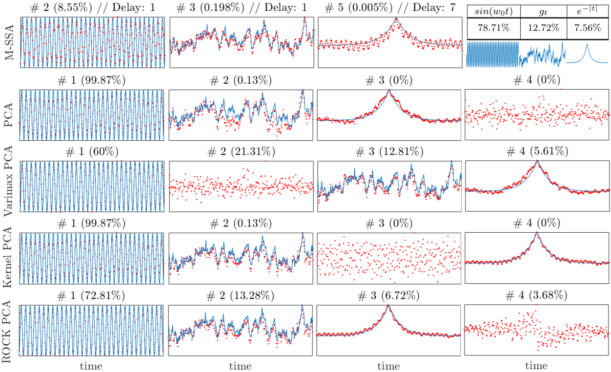
Figure 1: Comparison of dimensionality reduction methods (M-SSA, PCA, Varimax PCA, kernel PCA and the proposed ROCK-PCA) in the example of section III-C. We show the estimated time series in red and the original signal that better correlates in blue, and indicate the explained variance (in %, top), as well as theoretical variance per signal in the composition in the right top table. Time series without blue lines represent signals with high variance but unrelated with the original signals.

III-C Synthetic spatio-temporal experiments

This section illustrates and compares ROCK-PCA to other similar methods in literature. Let us define the following toy example:

$$f(x,y,t)=e^{-|t|}cos(kr)+g_{t}cos(ky)+sin(kxy-w_{0}t),$$

which represents a spatio-temporal signal with three additive time series ($e^{-|t|}$, $sin(w_{0})$ and $g_{t}$) and distinct spatial dynamics, and where $r=\sqrt{x^{2}+y^{2}}$, and $g_{t}=-\alpha g_{t-1}+e_{t}$ is an auto-regressive (AR) model, being $k=0.5$ rad/m, $w_{0}=4.5$ rad/s and $\alpha=2$.

Figure 2 shows the evolution of the kurtosis for the three optimization parameters in ROCK-PCA: the kernel hyperparameter $\sigma$, the Promax power $p$ and the number of extracted components $c$. Results confirm the robustness of the maximum kurtosis criterion to attain a stable solution in an unsupervised manner. In general, $c$ and $p$ response curves are less sensible than $\sigma$, and present clear local maxima. Choosing high $\sigma$ values means tending towards a linear solution as expected  [16]. In this case, there is a maximum at a relatively small $\sigma$ value, which suggests that the problem has a nonlinear solution.

	Kernel $\sigma\times 10^{4}$	Power $p$	Components $c$

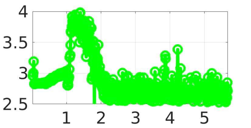
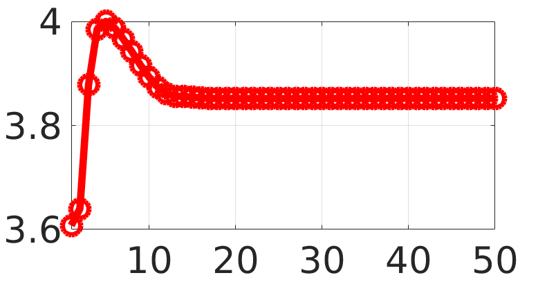
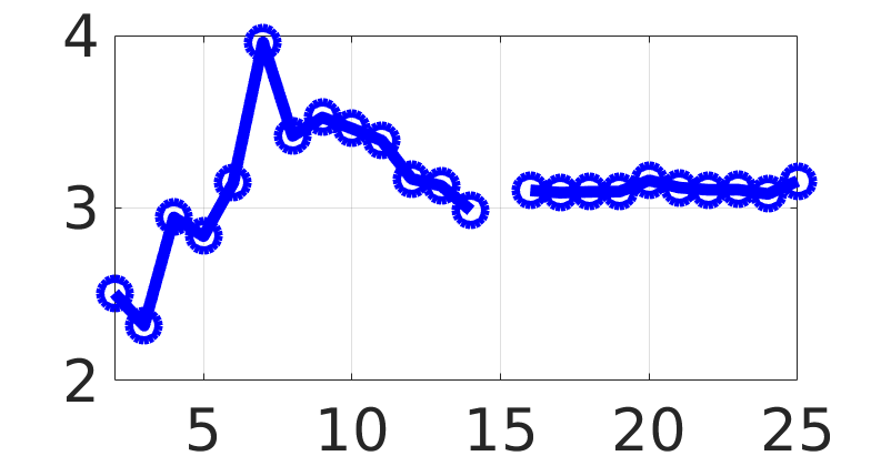
Figure 2: Kurtosis response curve for the three method parameters: kernel hyperparameter $\sigma$, Promax power $p$ and number of extracted components $c$.

	Original data		MSSA	ROCK-PCA
$sin(kxy)$		—————————–
$cos(ky)$		—————————–
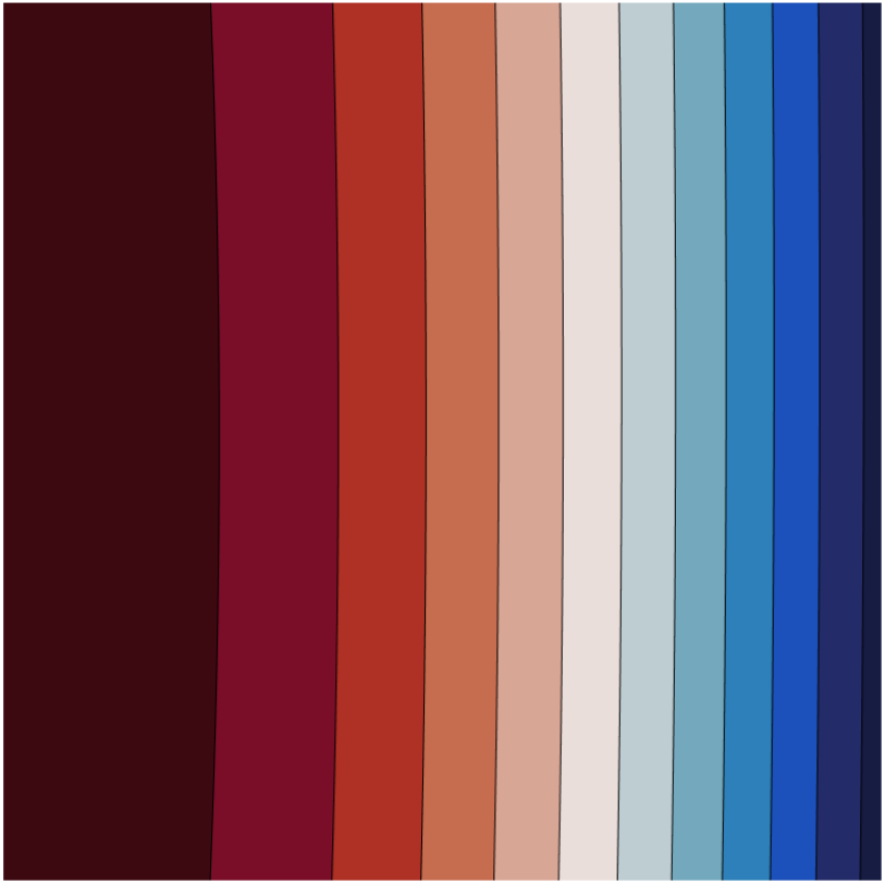
$cos(kr)$		—————————–

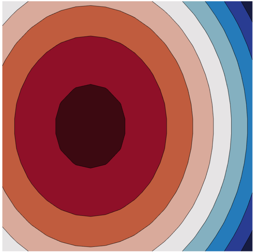
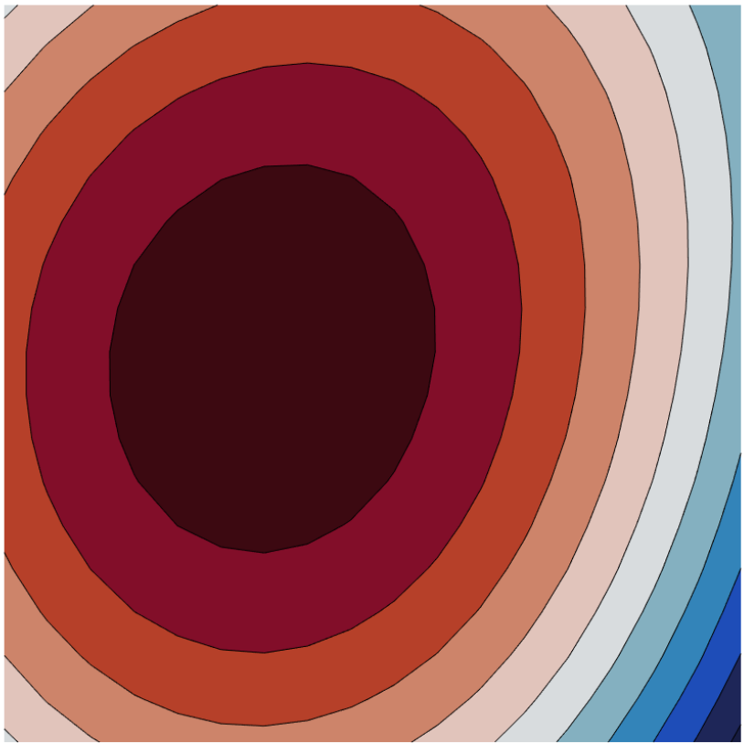
Figure 3: Spatial covariation patterns from estimated time series for the original signals (left), MSSA method (middle) and the proposed method (right).

Figure  1 shows the results of applying PCA, varimax PCA, MSSA, kernel PCA and our proposed method ROCK-PCA. All methods are able to decompose a linear separable data set and yield components sorted according to their signal variances. Regular PCA, however, cannot find the pure sinusoidal temporal mode and therefore cannot decompose the data correctly. A common alternative to PCA is the addition of a Varimax rotation. Note that the solution provided by Varimax, even though it regroups variability, the second component accounts for $21.31\%$ overall variance but it is unrelated with the original signal (see table in the top right). Multivariate Singular Spectral Analysis (MSSA) [52] efficiently identifies the three components, yet an intensive search over the lag parameter was needed over the second component. Results indicate that MSSA cannot reconstruct a robust set of time series with an interpretable explained variance. Our proposed ROCK-PCA method reproduces properly the real variances, its decomposition is not contaminated by components unrelated with the original signals (the top three components match the intrinsic components, and account for $92.81\%$ of the variance), and describes perfectly the input data.

More accurate explained variance and sharper components are clearly extracted by our method, especially when nonlinear processes are involved, such as for the $sin(w_{0}t)$ and $\exp(-|t|)$ components, while no differences are observed for the simpler autoregressive process. Besides, ROCK-PCA does not need to post-process the components by lag adjustment. Figure 3 shows the spatial covariation patterns. The ROCK-PCA patterns represent the real part of the complex estimation. ROCK-PCA spatial patterns better reflect the original spatial patterns unlike on MSSA spatial patterns.

IV Experimental results

The main goal of the proposed method is to extract information about relevant natural sub-processes that, although captured or modeled in Earth system products, are hidden under the variability of stronger modes such as the seasonal or the annual trends. The total variability of a signal -including minor but relevant modes– can be represented as a combination of components or modes with different temporal scales (e.g. interannual trends, seasonal resonances and anomalies) and spatial patterns.

In subsection A we illustrate the spatio-temporal feature extraction capability with GPP and SM data. In subsection B we show the complex spatial skills with SST data.

IV-A Spatio-temporal variability recognition

We here present experiments with two essential climate variables (ECVs): global Gross Primary Production (GPP) and Surface Soil Moisture (SM). We present their respective spatial and temporal decompositions with ROCK-PCA, and use the MODIS IGBP land cover classification [53] and the Köppen-Geiger climate classification [54] for interpretation of results.

Both GPP and SM data sets are defined in a regular grid, and are restricted to latitudes lower than 60^∘. The extracted components include two pieces of information: a temporal feature in the complex domain (with magnitude and phase) that accounts for the subprocesses explaining the temporal dynamic variability, and its corresponding spatial covariation which accounts for its spatial amplitude and phase. The spatial amplitude is useful to identify regions where the dominant mode is substantial. Using as significance threshold the median of the spatial amplitude with one positive standard deviation, we can mask the significant regions for each variability mode. The used range for the parameters is the same for all experiments. Maximum promax power $p^{*}$ is set on $10$ and the maximum number of components $c^{*}$ is set on 20. Hyperparameter $\sigma^{*}$ is searched in a range between 0.1 of the mean distance and 10 of maximum distance among all examples.

IV-A1 Global GPP decomposition

Gross primary productivity (GPP) is defined as the overall rate of fixation of carbon through the process of vegetation photosynthesis. It is a key parameter for carbon cycle and climate change research. It is used to quantify the amount of biomass (Carbon mass) produced within an ecosystem over a unit of time and is usually expressed in units of $gC/m^{2}/day$. Quantitative estimates of the spatial and temporal distribution of GPP at regional and global scales are essential for understanding the ecosystems response to increased atmospheric CO₂ level, and are thus critical for sustainability and decision making. A major contribution of CO₂ variability comes from GPP, as the photosynthesis process is vulnerable to droughts, heatwaves, floods, frost and other types of disturbances [55, 56, 57]. Here, we consider the GPP FLUXCOM product, obtained by upscaling FLUXNET [58] eddy-covariance observations by machine learning regression methods [59, 60, 61]. The FLUXCOM GPP product has global coverage and is provided as an eight-day composite with and spatial resolution of 5 arc-minutes ($\sim$10 Km).

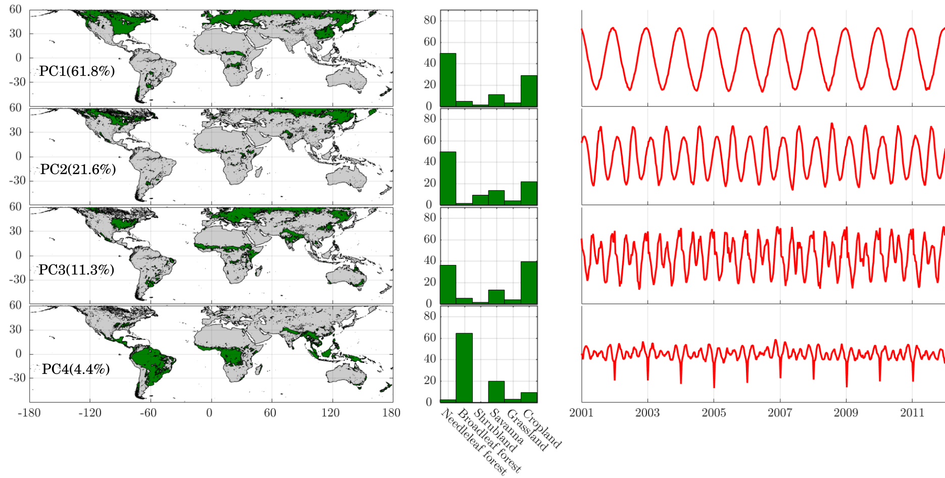
Figure 4: Global GPP decomposition results. Left: Spatial covariation for each component, which shows the spatial distribution of the amplitude signal. Middle: Composition of each extracted components in terms of vegetation land cover classification. Right: component as representative time series of each dynamic process. Vegetation regions differentiation is shown as well, and their common dynamics as for example croplands and needle leaf forest with oscillation periods of 12, 6 and 4 months.

Figure 4 shows the ROCK-PCA decomposition results for GPP data from years 2001 to 2012. A total of six components are identified, with the 99.1% explained variance being contained in the first four. The MODIS IGBP global land cover classification is used to spatially compare the distribution of the extracted modes among main Earth’s vegetation types. A visual examination of Figure 4 reveals the annual oscillation (first component) is stronger at high latitudes and equatorial zones. This responds to the high variability of the freezed latitudes, which are annually coupled with the variability at the equator. The second temporal component shows a six-month seasonality with a similar spatialization that represents subcycles of vegetation as monsoon oscillations. This result illustrates that ROCK-PCA is able to extract two different types of dynamics from similar regions, owing to the oblique rotation approach. The first and second components capture mainly the needleleaf forest variability and, to a lesser extent, the variability of certain croplands with related climatic conditions i.e. crops which phenology is characterized by a short period of Gross Primary Production stopped by the boreal/austral winter [62]. The third component covers major croplands, defined as a combination of a six-, four- and three-month periodic oscillation, resulting from the distinct growing season length of global agro-ecosystems, characterized by the crop type(s), planting and harvesting times, managerial activities and crop rotation techniques  [63]. The tropical vegetation is captured by the fourth temporal component. It represents the well-known GPP variance of tropical broadleaf forests, where the peak indicates their depletion during the spring season [64]. Note that inside each GPP mode, we capture all plant diversity, assuming equatorial and boreal homogeneous representation in a single dynamical mode, representing a multi-composed time series. A relevant result is that the majority of the variance (99.1%) is represented in the top four components which cover global vegetation seasonal dynamics. Short-term and inter-annual variability is represented by the fifth and sixth components, which account for approximately the 0.9% of the explained variance of the global GPP (not shown).

IV-A2 Global SM decomposition

Figure 5 shows the decomposition of the global Soil Moisture (SM) product from the SMOS Barcelona Expert Center (BEC). Since its launch in 2010, SMOS provides global maps of the Earth’s surface soil moisture (top 5 cm) every 3-days with a spatial resolution of $\sim$50 km and a target accuracy of 0.04 m${}^{3}\cdot$m^-3. For this work, we selected the first seven years of SMOS observations, after its commissioning phase (from May 2010 to May 2017). Soil Moisture is an ECV closely related with other relevant land climate variables as surface temperature or vegetation indexes. Knowledge of the spatio-temporal distribution of global SM and its changes is crucial for hydrological, ecological and climate models. It links the water and energy cycles over land and is an important driver of ecosystem variability  [65, 66].

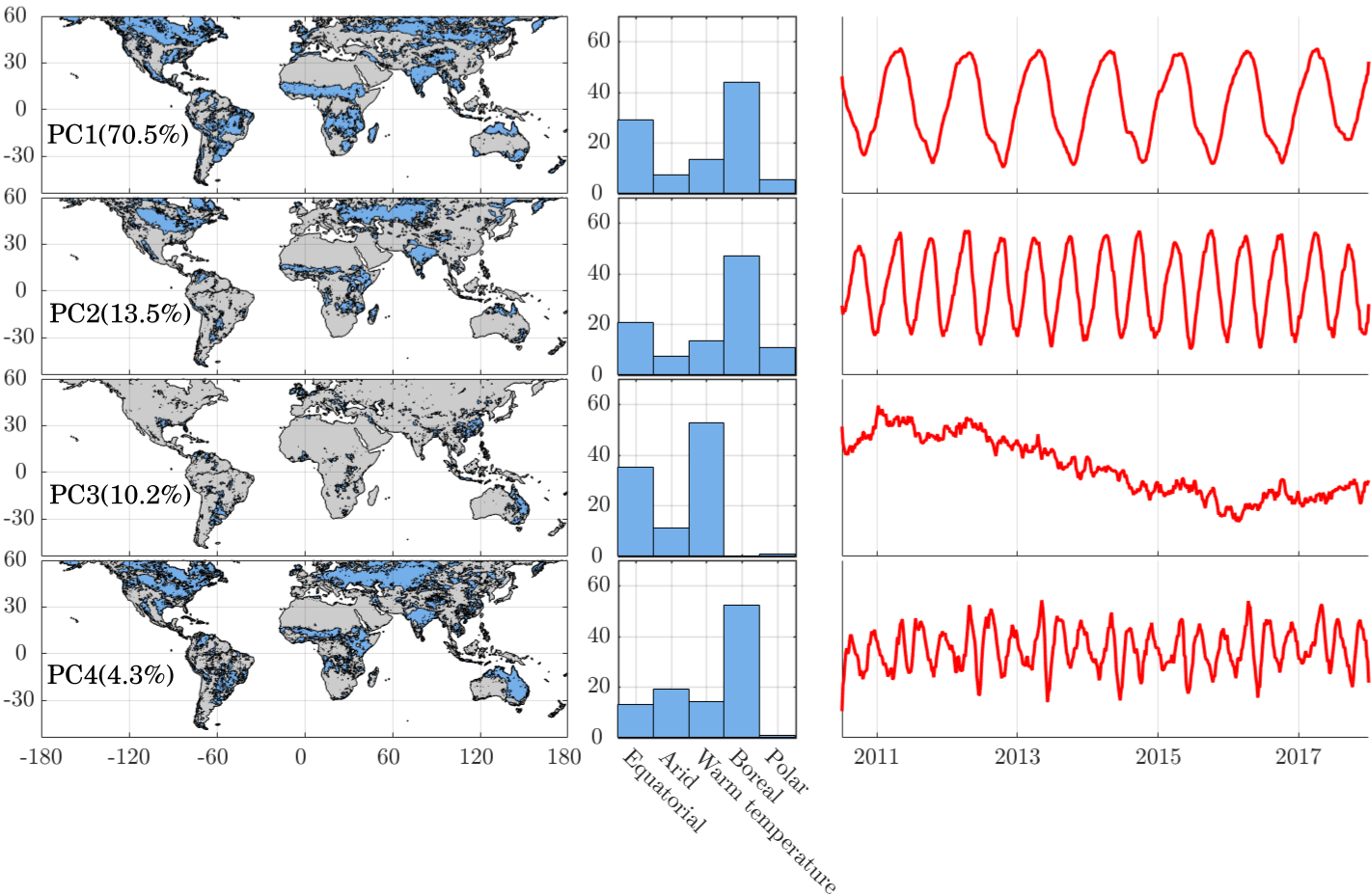
Figure 5: Global SM decomposition results. Left: Spatial covariation for each component, which shows the spatial distribution of the amplitude signal masked by significant amplitude. Middle: Composition of each extracted component in terms of KG global climate regions classification. Right: Temporal components of each dynamic process. Different time scales is show as annual, seasonal and interannual trends as well, classified in the principal climate regions.

The application of ROCK-PCA to the SM product yielded an optimal decomposition with seven components. The explained variance of the top four components accounts for $98.5\%$ of the overall variance, in line with a previous study focused in the spectrum of SM and its compression [67]. As we show in Fig. 5, the first component (70.5%) returns an annual oscillation with a $12$-month period and a global spatial distribution, it represent the dominant mode of annual SM variability. The second (13.5%) and fourth components (4.3%) are cast as ‘resonances’ of the annual SM cycle with six- and four-month periods, respectively, which correspond to subcycles of global SM as the Inter-tropical Convergence Zone (ITCZ) oscillation (second component) or the seasonal transition (fourth component). First, second and fourth components contain tropical monsoon oscillations, representing periodic sub-annual processes.

Interestingly, the third component (10.2%) shows a non-seasonal oscillation with a large period of about $4.5$ years which can be interpreted as a long-term change in the global SM distribution. Comparing the spatial distribution of the amplitudes with the Köppel-Geiger climate classification [54], we can see that the annual and the half-year oscillation (first and second component) are distributed mostly in tropical latitudes and high latitudes, representing the oscillation of ice-covered lands. The fourth component partially contains these regions and also includes the transition between arid and wet regions. The inter-annual component is widely related with warmer (and wetter) regions representing approximately the 10.2% of total global variability, and highlight the role of these regions as hot-spots for climate change research. These dry/wet regions reproduce the well-known ENSO anomalies ($2-8$ years [68]) induced precipitation patterns [15, 69, 70], and teleconnections [5]. This remarks the close relation of satellite-based global soil moisture variability with ENSO, in line with previous research [71, 10, 72, 73].

IV-B Nonlinear phase dynamics for SST and ENSO analysis

The proposed method works in the complex plane so magnitude as well as phase components can be extracted. We illustrate this capability with the decomposition of global Sea Surface Temperatures (SST) from the MetOffice renalysis HadISST1  [74]. We used a global SST $1^{\circ}$ gridded and monthly sampled cube between years 1871-2014. We focus on latitudes lower than $45^{\circ}$ and center the analysis in tropical and middle latitudes dynamics. This is customary to avoid interference of other variables, such as the ice cover variability in high latitudes that otherwise masks the SST dynamics of middle latitudes.

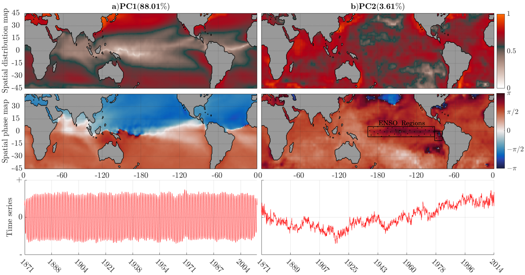
Figure 6: Global SST decomposition results. Spatial distribution of the first (a) and second (b) components for both the spatial covariation amplitude normalized to one (top row), the spatial covariation phase (middle row), and the temporal component (bottom row). ENSO regions are also shown.

Figure 6 shows the obtained spatio-temporal decomposition in magnitude and phase. A total of five features accounted for 99.8% of the variance. The first component shows clearly the annual north-south oscillation (88.01%), while the second component is more related to the interdecadal variability (3.61%). The Three following components are related to inter-annual variability as different ENSO anomalies, they are modes third to fifth representing 8.18% variability (not shown). We focus here on the magnitude-phase characteristics of the first two components and their relation with ENSO, leaving the study of the inter-annual components for further studies. It can be seen that the spatial amplitude and phase of the selected components uncover extra dynamical patterns, such as for example the annual oscillation (first component) which is represented by a two opposed-phase regions conforming a north-south oscillation boundary, representing faithfully the ITCZ line and its annual displacement (see Fig. 6.a). The second component represents the inter-decadal temperature trend, where we can observe the recent rise of global SST with an approximate homogeneous spatial distribution that can be interpreted as the sea global warming (SGW) [75]. Interestingly, the phase map shows that the ENSO region is disturbed by a positive phase in opposition to the rest of the oceans, which suggests a positive phase coupling between ENSO and SGW. This is further analyzed in Fig. 7, representing a time dependence and, in extension, a variance dependence of ENSO events with SGW [76]. This shows well-known patterns where ENSO events variability are related with the ocean temperature raise but with a positive time delay [77, 78, 12]. Note that in negative phases (respectively, cooling regions), there is generally a low amplitude response.

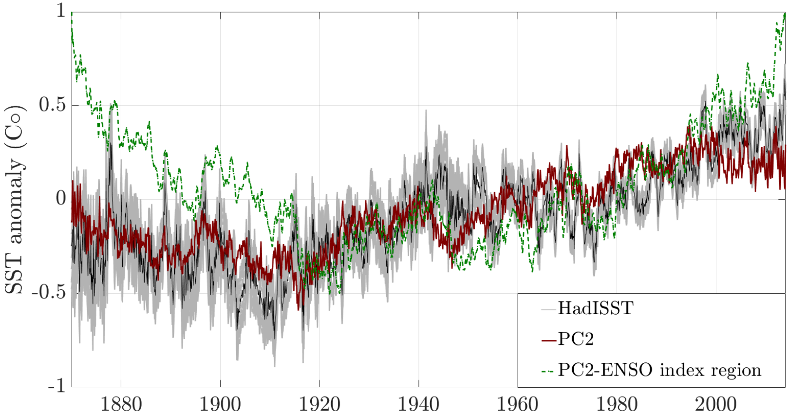
Figure 7: Comparison of inter-decadal trends of SST: mean SST Had1SST product (black line with +/- standard deviation in shaded gray), average of the second mode of variability obtained with ROCK-PCA (PC2, red line), average of PC2 extracted from ENSO index regions in Fig.6 (green line). The SST Had1SST product is highly correlated with the total average of the second variability mode. The ENSO-region SST presents a different variability trend and a lagged response with respect to the other two.

V Conclusions

In this paper we proposed a nonlinear dimensionality reduction method for spatial-temporal analysis of Earth observation data. The proposed method is based on kernel methods to deal with nonlinear processes and feature relations, it operates in the complex kernel domain to account for both space and time features, and adds an extra rotation that makes the components non-orthogonal to allow recovering correlated features. The method is also very efficient computationally since it can work in the dual space, which is convenient in the usual case where the amount of available pixels is larger than the number of temporal observations. If we encounter the contrary case, the formulation could be easily adapted to work in the primal for efficiency. The method contains three parameters to tune: kernel parameter, shape of the rotation transform, and number of components to extract. To make the method unsupervised and less sensible to their selection, we proposed the optimization of the fourth moment (kurtosis) of the distribution of projections, following similar motivations in ICA approaches to signal decomposition.

We showed performance in synthetic experiments, and three real data cubes involving land and ocean applications: global GPP, SM, and SST. The method allows identifying in a general way, annual and seasonal oscillations, as well as their non-seasonal trends and spatial variability patterns. The main modes of variation of GPP and SM are shown to match expected distributions of land-cover and eco-hydrological zones, respectively; GPP decomposition represents faithfully the principal vegetation land cover dynamics in a compressed way; the spatialization of the inter-annual component of SM reproduce accurately the global ENSO teleconnection patterns and possible novel dry/wet patterns; the SST annual oscillation is perfectly uncoupled in magnitude and phase from the global warming trend and ENSO anomalies, showing his mutual interaction as ENSO and global warming trend coupled system.

One of the current limitations is that the input data set has to be sampled on a regular grid in space and time, so it cannot properly performed with gaps in the data. Some alternatives exist in the literature to resolve this, such as gap-filling the data, missing-data PCA methods, or more recent approaches based on graphs. Given our kernel-based approach, replacing the kernel matrix with a graph Laplacian would allow to resolve this problem in an elegant way. Recent literature has actually combined Laplacian eigenmaps with Takens embedding for spatio-temporal data analysis [79], which we will explore in the future too. Interestingly, note that ROCK-PCA extracts meaningful features even without a time embedding.

Perhaps the most important limitation is about the interpretability of the results, as it is definitively challenging to identify first the number of components which describe the data well and then to assign them to particular physical processes and events. While we propose here the use of kurtosis as a sensible criterion for the first, the physical interpretation (and eventual teleconnections) of the extracted components is still an unsolved problem and matter of current and active research.

It is acknowledged that the method is general enough to work with arbitrary spatio-temporal data. The method is applicable to all kind of variables, and generalizable to work with multiple variables, not just a single one  [80]. We foresee a wide range of applications to exploit the gridded information in Earth cube initiatives, such as the Earth System Data Cube (ESDC). Spatio-temporal data structures are not only encountered in Earth sciences. We anticipate applications of the method in many other fields: from epidemics, neurosciences, social sciences to economics.

References

- [1] N. B. Guttman, “Statistical descriptors of climate,” Bulletin of the American Meteorological Society, vol. 70, no. 6, pp. 602–607, 1989.
- [2] J. W. Larson, “Can we define climate using information theory?” IOP Conference Series: Earth and Environmental Science, vol. 11, no. 1, p. 012028, 2010.
- [3] D. Dong, P. Fang, Y. Bock, F. Webb, L. Prawirodirdjo, S. Kedar, and P. Jamason, “Spatiotemporal filtering using principal component analysis and Karhunen-Loeve expansion approaches for regional GPS network analysis,” Journal of Geophysical Research: Solid Earth, vol. 111, no. B3.
- [4] M. Gehne, R. Kleeman, and K. E. Trenberth, “Irregularity and decadal variation in ENSO: a simplified model based on Principal Oscillation Patterns,” Climate Dynamics, vol. 43, no. 12, pp. 3327–3350, Dec 2014.
- [5] S. Brands, “Which ENSO teleconnections are robust to internal atmospheric variability?” Geophysical Research Letters, vol. 44, no. 3, pp. 1483–1493, 2017.
- [6] D. P. Mandic, N. u. Rehman, Z. Wu, and N. E. Huang, “Empirical mode decomposition-based time-frequency analysis of multivariate signals: The power of adaptive data analysis,” IEEE Signal Processing Magazine, vol. 30, no. 6, pp. 74–86, Nov 2013.
- [7] Y. Zhao, L. Wang, T. Huang, J. Mo, X. Zhang, H. Gao, and J. Ma, “Feature extraction of climate variability, seasonality, and long-term change signals in persistent organic pollutants over the Arctic and the great lakes,” Journal of Geophysical Research: Atmospheres, vol. 122, no. 16, pp. 8921–8939, 2017.
- [8] E. Forootan, Khandu, J. Awange, M. Schumacher, R. Anyah, A. V. Dijk, and J. Kusche, “Quantifying the impacts of ENSO and IOD on rain gauge and remotely sensed precipitation products over Australia,” Remote Sensing of Environment, vol. 172, 2016.
- [9] D. L. Volkov, “Do the North Atlantic winds drive the nonseasonal variability of the Arctic Ocean sea level?” Geophysical Research Letters, vol. 41, no. 6, 2014.
- [10] B. Bauer-Marschallinger, W. A. Dorigo, W. Wagner, and A. I. J. M. V. Dijk, “How oceanic oscillation drives soil moisture variations over mainland Australia: An analysis of 32 years of satellite observations,” Journal of Climate, vol. 26, no. 24, 2013.
- [11] T. Lian and D. Chen, “An evaluation of rotated EOF analysis and its application to tropical pacific SST variability,” Journal of Climate, vol. 25, no. 15, 2012.
- [12] X. Chen, J. M. Wallace, and K.-K. Tung, “Pairwise-rotated eofs of global sst,” Journal of Climate, vol. 30, no. 14, pp. 5473–5489, 2017.
- [13] E. Rousi, C. Anagnostopoulou, K. Tolika, and P. Maheras, “Representing teleconnection patterns over Europe: A comparison of SOM and PCA methods,” Atmospheric Research, vol. 152, pp. 123 – 137, 2015, atmospheric Processes in the Mediterranean.
- [14] D. Mukhin, A. Gavrilov, A. Feigin, E. Loskutov, and J. Kurths, “Principal nonlinear dynamical modes of climate variability,” Scientific Reports, vol. 5, 2015.
- [15] A. Dai and T. M. L. Wigley, “Global patterns of ENSO-induced precipitation,” Geophysical Research Letters, vol. 27, no. 9, pp. 1283–1286, 2000.
- [16] G. Camps-Valls and L. Bruzzone, Eds., Kernel methods for remote sensing data analysis. UK: Wiley & Sons, Dec 2009.
- [17] J. Arenas-García, K. Petersen, G. Camps-Valls, and L. Hansen, “Kernel multivariate analysis framework for supervised subspace learning: A tutorial on linear and kernel multivariate methods,” IEEE Signal Processing Magazine, vol. 30, no. 4, pp. 16–29, 2013.
- [18] J. Runge, V. Petoukhov, J. F. Donges, J. Hlinka, N. Jajcay, M. Vejmelka, D. Hartman, N. Marwan, M. Paluš, J. Kurths, and et al., “Identifying causal gateways and mediators in complex spatio-temporal systems,” Nature Communications, vol. 6, no. 1, Jul 2015.
- [19] B. Wa, Z. Wu, J. Li, J. Liu, C.-P. Chang, Y. Ding, and G. Wu, “How to measure the strength of the East Asian summer Monsoon,” Journal of Climate, vol. 21, no. 17, pp. 4449–4463, 2008.
- [20] A. Hannachi, I. T. Jolliffe, and D. B. Stephenson, “Empirical Orthogonal Functions and related techniques in atmospheric science: A review,” International Journal of Climatology, vol. 27, no. 9, pp. 1119–1152, 2007.
- [21] M. D. Mahecha, L. M. Fürst, N. Gobron, and H. Lange, “Identifying multiple spatiotemporal patterns: A refined view on terrestrial photosynthetic activity,” Pattern Recognition Letters, vol. 31, no. 14, pp. 2309 – 2317, 2010.
- [22] C. Liu, S. Ray, G. Hooker, and M. Friedl, “Functional factor analysis for periodic remote sensing data,” The Annals of Applied Statistics, vol. 6, no. 2, p. 601–624, 2012.
- [23] F. Cremer, M. Urbazaev, C. Berger, M. D. Mahecha, C. Schmullius, and C. Thiel, “An image transform based on temporal decomposition,” IEEE Geoscience and Remote Sensing Letters, vol. 15, no. 4, pp. 537–541, April 2018.
- [24] S. M. Hirsh, B. W. Brunton, and J. N. Kutz, “Data-driven Spatiotemporal Modal Decomposition for Time Frequency Analysis,” ArXiv e-prints, Jun. 2018.
- [25] S. Le Clainche and J. Vega, “Spatio-temporal Koopman decomposition,” Journal of Nonlinear Science, vol. 28, pp. 1–50, 05 2018.
- [26] J. Luttinen and A. Ilin, “Variational gaussian-process factor analysis for modeling spatio-temporal data,” in Advances in Neural Information Processing Systems 22, Y. Bengio, D. Schuurmans, J. D. Lafferty, C. K. I. Williams, and A. Culotta, Eds. Curran Associates, Inc., 2009, pp. 1177–1185.
- [27] R. Yu, D. Cheng, and Y. Liu, “Accelerated online low-rank tensor learning for multivariate spatio-temporal streams,” in Proceedings of the 32Nd International Conference on International Conference on Machine Learning - Volume 37, 2015, pp. 238–247.
- [28] H. A. Dijkstra, Nonlinear Climate Dynamics. Cambridge University Press, 2013.
- [29] N. Cristianini and B. Schölkopf, “Support vector machines and kernel methods: The new generation of learning machines,” AI Mag., vol. 23, no. 3, pp. 31–41, Sep. 2002.
- [30] G. Camps-Valls, J. Benediktsson, L. Bruzzone, and J. Chanussot, “Introduction to the issue on advances in remote sensing image processing,” IEEE Journal of Selected Topics in Signal Processing, vol. 5, no. 3, pp. 365–369, Jun 2011.
- [31] H. F. Kaiser, “The varimax criterion for analytic rotation in factor analysis,” Psychometrika, vol. 23, no. 3, p. 187–200, 1958.
- [32] A. E. Hendrickson and P. O. White, “Promax: A quick method for rotation to oblique simple structure,” British Journal of Statistical Psychology, vol. 17, no. 1, p. 65–70, 1964.
- [33] P. Esquivel and A. R. Messina, “Complex empirical orthogonal function analysis of wide-area system dynamics,” 2008 IEEE Power and Energy Society General Meeting - Conversion and Delivery of Electrical Energy in the 21st Century, 2008.
- [34] J. D. Horel, “Complex principal component analysis: Theory and examples,” Journal of Climate and Applied Meteorology, vol. 23, no. 12, 1984.
- [35] C. Rusu, P. Kuosmanen, and J. Astola, “Hilbert transform of discrete data: a brief review,” in Proceedings of The 2005 International TICSP Workshop on Spectral Methods and Multirate Signal Processing, 2005, pp. 79–84.
- [36] E. Boergens, E. Rangelova, M. G. Sideris, and J. Kusche, “Assessment of the capabilities of the temporal and spatiotemporal ICA method for geophysical signal separation in GRACE data,” Journal of Geophysical Research: Solid Earth, vol. 119, no. 5, pp. 4429–4447, 2013.
- [37] A. Sharma and K. K. Paliwal, “Fast principal component analysis using fixed-point algorithm,” Pattern Recognition Letters, vol. 28, no. 10, 2007.
- [38] C. M. Bishop, Pattern Recognition and Machine Learning. Springer, 2006.
- [39] T. R. Karl, A. J. Koscielny, and H. F. Diaz, “Potential errors in the application of principal component (eigenvector) analysis to geophysical data,” Journal of Applied Meteorology, vol. 21, no. 8, 1982.
- [40] B. Schölkopf, A. Smola, and K.-R. Müller, “Nonlinear component analysis as a kernel eigenvalue problem,” Neural Computation, vol. 10, no. 5, p. 1299–1319, 1998.
- [41] P. Bouboulis and S. Theodoridis, “Extension of wirtingers calculus to reproducing kernel hilbert spaces and the complex kernel LMS,” IEEE Transactions on Signal Processing, vol. 59, no. 3, p. 964–978, 2011.
- [42] J. Rojo-Álvarez, M. Martínez-Ramón, J. Muñoz-Marí, and G. Camps-Valls, Digital Signal Processing with Kernel Methods. UK: Wiley & Sons, Apr 2017.
- [43] J. Miettinen, S. Taskinen, K. Nordhausen, and H. Oja, “Fourth moments and independent component analysis,” Statist. Sci., vol. 30, no. 3, pp. 372–390, 08 2015.
- [44] J. F. Cardoso, “Source separation using higher order moments,” in International Conference on Acoustics, Speech, and Signal Processing,, May 1989, pp. 2109–2112 vol.4.
- [45] D. Peña and F. J. Prieto, “Cluster identification using projections,” Journal of the American Statistical Association, vol. 96, no. 456, pp. 1433–1445, 2001.
- [46] ——, “Multivariate outlier detection and robust covariance matrix estimation,” Technometrics, vol. 43, no. 3, pp. 306–310, 2001.
- [47] M. Castella and E. Moreau, “A new method for kurtosis maximization and source separation,” 2010 IEEE International Conference on Acoustics, Speech and Signal Processing, 2010.
- [48] M. van der Baan and S. Fomel, “Nonstationary phase estimation using regularized local kurtosis maximization,” Geophysics, 2009.
- [49] L. T. DeCarlo, “On the meaning and use of kurtosis,” Psychological Methods, vol. 2, no. 3, pp. 292–307, 1997.
- [50] G. Bakir, J. Weston, and B. Schölkopf, “Learning to find pre-images,” in NIPS 16. MIT Press, 2003.
- [51] J. T. Kwok and I. W. Tsang, “The pre-image problem in kernel methods,” IEEE Trans. Neural Networks, vol. 15, no. 6, pp. 1517–1525, 2004.
- [52] N. Golyandina, V. Nekrutkin, and A. Zhigljavsky, Analysis of Time Series Structure: SSA and Related Techniques, 2001.
- [53] M. A., Friedl, D. Sulla-Menashe, B. Tan, A. Schneider, N. Ramankutty, A. Sibley and X. Huang. (2010) MODIS collection 5 global land cover: Algorithm refinements and characterization of new datasets, 2001-2012, collection 5.1 IGBP land cover. [Online]. Available: http://www.landcover.org/
- [54] Kottek, M., J. Grieser, C. Beck, B. Rudolf, and F. Rubel. (2006) World map of the Köppen-Geiger climate classification updated. [Online]. Available: http://koeppen-geiger.vu-wien.ac.at/present.htm
- [55] C. Beer, M. Reichstein, E. Tomelleri, P. Ciais, M. Jung, N. Carvalhais, C. Rödenbeck, M. A. Arain, D. Baldocchi, G. B. Bonan, A. Bondeau, A. Cescatti, G. Lasslop, A. Lindroth, M. Lomas, S. Luyssaert, H. Margolis, K. W. Oleson, O. Roupsard, E. Veenendaal, N. Viovy, C. Williams, F. I. Woodward, and D. Papale, “Terrestrial gross carbon dioxide uptake: Global distribution and covariation with climate,” Science, vol. 329, no. 5993, pp. 834–838, 2010.
- [56] M. Jung, M. Reichstein, H. A. Margolis, A. Cescatti, A. D. Richardson, M. A. Arain, A. Arneth, C. Bernhofer, D. Bonal, J. Chen, D. Gianelle, N. Gobron, G. Kiely, W. Kutsch, G. Lasslop, B. E. Law, A. Lindroth, L. Merbold, L. Montagnani, E. J. Moors, D. Papale, M. Sottocornola, F. Vaccari, and C. Williams, “Global patterns of land-atmosphere fluxes of carbon dioxide, latent heat, and sensible heat derived from eddy covariance, satellite, and meteorological observations,” Journal of Geophysical Research: Biogeosciences, vol. 116, no. G3, 2011.
- [57] M. Jung, M. Reichstein, C. R. Schwalm, C. Huntingford, S. Sitch, A. Ahlström, A. Arneth, G. Camps-Valls, P. Ciais, P. Friedlingstein, F. Gans, K. Ichii, A. K. Jain, E. Kato, D. Papale, B. Poulter, B. Raduly, C. Rödenbeck, G. Tramontana, N. Viovy, Y.-P. Wang, U. Weber, S. Zaehle, and N. Zeng, “Compensatory water effects link yearly global land CO2 sink changes to temperature,” Nature, vol. 541, no. 7638, pp. 516–520, Jan 2017.
- [58] FLUXCOM Global Energy and Carbon Fluxes. (2018) Max planck institute for biogeochemistry, Jena, Germany. [Online]. Available: http://www.fluxcom.org/
- [59] G. Tramontana, M. Jung, G. Camps-Valls, K. Ichii, B. Raduly, M. Reichstein, C. R. Schwalm, M. A. Arain, A. Cescatti, G. Kiely, L. Merbold, P. Serrano-Ortiz, S. Sickert, S. Wolf, and D. Papale, “Predicting carbon dioxide and energy fluxes across global fluxnet sites with regression algorithms,” Biogeosciences Discussions, vol. 2016, pp. 1–33, 2016.
- [60] G. Tramontana, K. Ichii, G. Camps-Valls, E. Tomelleri, and D. Papale, “Uncertainty analysis of gross primary production upscaling using random forests, remote sensing and eddy covariance data,” Remote Sensing of Environment, vol. 168, pp. 360 – 373, 2015.
- [61] G. Camps-Valls, M. Jung, K. Ichii, D. Papale, G. Tramontana, P. Bodesheim, C. Schwalm, J. Zscheischler, M. Mahecha, and M. Reichstein, “Ranking drivers of global carbon and energy fluxes over land,” Geoscience and Remote Sensing Symposium (IGARSS), 2015 IEEE International, 2015.
- [62] B. Byrne, D. Wunch, D. B. A. Jones, K. Strong, F. Deng, I. Baker, P. Köhler, C. Frankenberg, J. Joiner, V. K. Arora, B. Badawy, A. B. Harper, T. Warneke, C. Petri, R. Kivi, and C. M. Roehl, “Evaluating GPP and respiration estimates over northern midlatitude ecosystems using solar-induced fluorescence and atmospheric CO2 measurements,” Journal of Geophysical Research: Biogeosciences, vol. 123, no. 9, pp. 2976–2997, 2018.
- [63] A. Noormets and J. Chen and L. Gu and A. Desai, Phenology of Ecosystem Processes. Springer, 2009.
- [64] L. Xu and S. S. Saatchi and Y. Yang and R. B. Myneni and C. Frankenberg and D. Chowdhury and J. Bi, “Satellite observation of tropical forest seasonality: spatial patterns of carbon exchange in amazonia,” Environmental Research Letters, vol. 10, no. 8, p. 084005, 2015.
- [65] S. I. Seneviratne, T. Corti, E. L. Davin, M. Hirschi, E. B. Jaeger, I. Lehner, B. Orlowsky, and A. J. Teuling, “Investigating soil moisture–climate interactions in a changing climate: A review,” Earth-Science Reviews, vol. 99, no. 3, pp. 125 – 161, 2010.
- [66] R. D. Koster, S. P. P. Mahanama, T. J. Yamada, G. Balsamo, A. A. Berg, M. Boisserie, P. A. Dirmeyer, F. J. Doblas-Reyes, G. Drewitt, C. T. Gordon, Z. Guo, J.-H. Jeong, W.-S. Lee, Z. Li, L. Luo, S. Malyshev, W. J. Merryfield, S. I. Seneviratne, T. Stanelle, B. J. J. M. van den Hurk, F. Vitart, and E. F. Wood, “The second phase of the global land–atmosphere coupling experiment: Soil moisture contributions to subseasonal forecast skill,” Journal of Hydrometeorology, vol. 12, no. 5, pp. 805–822, 2011.
- [67] G. G. Katul, A. Porporato, E. Daly, A. C. Oishi, H.-S. Kim, P. C. Stoy, J.-Y. Juang, and M. B. Siqueira, “On the spectrum of soil moisture from hourly to interannual scales,” Water Resources Research, vol. 43, no. 5, 2007.
- [68] L. Yuan, Z. Yu, Z. Xie, Z. Song, and G. Lü, “ENSO signals and their spatial-temporal variation characteristics recorded by the sea-level changes in the northwest pacific margin during 1965–2005,” Science in China Series D: Earth Sciences, vol. 52, no. 6, 2009.
- [69] B. Lyon and A. G. Barnston, “ENSO and the spatial extent of interannual precipitation extremes in tropical land areas,” Journal of Climate, vol. 18, no. 23, pp. 5095–5109, 2005.
- [70] S.-W. Yeh, W. Cai, S.-K. Min, M. J. McPhaden, D. Dommenget, B. Dewitte, M. Collins, K. Ashok, S.-I. An, B.-Y. Yim, and J.-S. Kug, “ENSO atmospheric teleconnections and their response to greenhouse gas forcing,” Reviews of Geophysics, vol. 56, no. 1, pp. 185–206, 2018.
- [71] D. G. Miralles, M. J. V. D. Berg, J. H. Gash, R. M. Parinussa, R. A. M. D. Jeu, H. E. Beck, T. R. H. Holmes, C. Jiménez, N. E. C. Verhoest, W. A. Dorigo, and et al., “EL NIÑOLA NIÑA cycle and recent trends in continental evaporation,” Nature Climate Change, vol. 4, no. 2, Aug 2013.
- [72] D. Bueso, M. Piles, and G. Camps-Valls, “Nonlinear Complex PCA for Spatio-Temporal Analysis of Global Soil Moisture ,” in 2018 IEEE International Geoscience and Remote Sensing Symposium, València, Spain, July 23-28 2018.
- [73] M. Piles, J. Ballabrera-Poy, and J. Muñoz Sabater, “Dominant Features of Global Surface Soil Moisture Variability Observed by the SMOS Satellite,” Remote Sensing, vol. 11, no. 1, 2019.
- [74] N. A. Rayner, D. E. Parker, E. B. Horton, C. K. Folland, L. V. Alexander, D. P. Rowell, E. C. Kent, and A. Kaplan, “Global analyses of sea surface temperature, sea ice, and night marine air temperature since the late nineteenth century,” Journal of Geophysical Research: Atmospheres, vol. 108, no. D14.
- [75] G. Foster and S. Rahmstorf, “Global temperature evolution 1979–2010,” Environmental Research Letters, vol. 6, no. 4, p. 044022, 2011.
- [76] Q. Zhang, Y. Guan, and H. Yang, “ENSO amplitude change in observation and coupled models,” Advances in Atmospheric Sciences, vol. 25, no. 3, pp. 361–366, May 2008.
- [77] D. W. J. Thompson, J. J. Kennedy, J. M. Wallace, and P. D. Jones, “A large discontinuity in the mid-twentieth century in observed global-mean surface temperature,” Nature, vol. 453, no. 646, 2008.
- [78] G. P. Compo and P. D. Sardeshmukh, “Removing ENSO-related variations from the climate record,” Journal of Climate, vol. 23, no. 8, pp. 1957–1978, 2010.
- [79] E. Székely, D. Giannakis, and A. J. Majda, “Extraction and predictability of coherent intraseasonal signals in infrared brightness temperature data,” Climate Dynamics, vol. 46, no. 5, pp. 1473–1502, Mar 2016.
- [80] S. Sparnocchia, N. Pinardi, and E. Demirov, “Multivariate empirical orthogonal function analysis of the upper thermocline structure of the mediterranean sea from observations and model simulations,” Annales Geophysicae, vol. 21, no. 1, pp. 167–187, 2003.