The $\pi\eta$ interaction and $a_{0}$ resonances in photon-photon scattering

Abstract

We revisit the information on the two lightest $a_{0}$ resonances and $S$-wave $\pi\eta$ scattering that can be extracted from photon-photon scattering experiments. For this purpose we construct a model for the $S$-wave photon-photon amplitudes which satisfies analyticity properties, two-channel unitarity and obeys the soft photon as well as the soft pion constraints. The underlying I=1 hadronic $T$-matrix involves six phenomenological parameters and is able to account for two resonances below 1.5 GeV. We perform a combined fit of the $\gamma\gamma\to\pi\eta$ and $\gamma\gamma\to K_{S}K_{S}$ high statistics experimental data from the Belle collaboration. Minimisation of the $\chi^{2}$ is found to have two distinct solutions with approximately equal $\chi^{2}$. One of these exhibits a light and narrow excited $a_{0}$ resonance analogous to the one found in the Belle analysis. This however requires a peculiar coincidence between the $J=0$ and $J=2$ resonance effects which is likely to be unphysical. In both solutions the $a_{0}(980)$ resonance appears as a pole on the second Riemann sheet. The location of this pole in the physical solution is determined to be $m-i\Gamma/2=1000.7^{+12.9}_{-0.7}-i\,36.6^{+12.7}_{-2.6}$ MeV. The solutions are also compared to experimental data in the kinematical region of the decay $\eta\to\pi^{0}\gamma\gamma$. In this region an isospin violating contribution associated with ${\pi^{+}}{\pi^{-}}$ rescattering must be added for which we provide a dispersive evaluation.

1 Introduction:

The $a_{0}(980)$ and $f_{0}(980)$ scalar mesons were the first observed members of a family of exotic resonances in QCD which are located very close to an inelastic two-particle (or quasi two-particle) threshold (see the review [1]). The $a_{0}(980)$ resonance was discovered a long time ago and seen in both the $K\bar{K}$ and the $\pi\eta$ channels [2, 3] but its properties are still imprecisely known. This is partly because $\pi\eta$ production experiments using an $\eta$ beam, analogous to those which have allowed to determine the $\pi\pi$ or $\pi K$ phase shifts, are not feasible. The $a_{0}(980)$ properties have to be determined solely from final-state rescattering effects. As shown by Flatté [4], who proposed a simple replacement for the Breit-Wigner resonance formula accounting for the $\pi\eta-K\bar{K}$ coupled-channel dynamics, ambiguous results for the $a_{0}$ width can be obtained. In the PDG [5], indeed, its width is simply quoted as lying in a range from 50 to 100 MeV. Beyond the value of the width, one would like to determine the positions of the poles on the unphysical Riemann sheets. For resonance states close to an inelastic threshold, there are three sheets (II, III, IV in the case of the $a_{0}$) which are physically relevant (i.e. a pole in one of these can be close to the physical region). It is also clear that a better determination of the resonance properties is closely tied to a better knowledge of the physical scattering $T$-matrix.

A theoretically motivated treatment of final-state interactions becomes prohibitively difficult for multiparticle final states. In this regard, photon-photon to meson-meson scattering amplitudes are very favourable processes.They are free of initial-state interactions and satisfy dispersion relations which can be constrained, in the case of $\pi\pi$ or $\pi\eta$ by both soft photon [7, 8] and soft pion [9] low-energy theorems. As was illustrated in the seminal papers [10, 11] a predictive representation can be implemented at the level of the partial-waves with a simple modelling of the left-hand cut. From an experimental point of view $\gamma\gamma\to\eta\pi^{0}$ cross-sections were first measured by the Crystal Ball collaboration [12]. Measurements with much higher statistics were recently performed by the Belle collaboration [13]. There are also experimental results on the $\eta\to\pi^{0}\gamma\gamma$ decay amplitude [14, 15]. Recent experimental data exist also for $\gamma\gamma\to{K^{0}}{\bar{K}^{0}}$ [16] and $\gamma\gamma\to{K^{+}}{K^{-}}$ [17] which will be considered in our study.

There are two puzzling aspects in the data analysis performed by the Belle collaboration which we wish to reconsider: a) they find that the $a_{0}(980)$ peak seems to be best described by an ordinary (i.e. essentially elastic) Breit-Wigner function and b) they find an excited $a_{0}$, which could correspond to the $a_{0}(1450)$, but has a width, $\Gamma=65^{+2.1}_{-5.4}$ MeV, much smaller than the PDG average as well as a significantly smaller mass. These data have been re-analysed recently [18] based on a specific meson-meson $T$-matrix model [19] applied to the $\pi\eta$ $S$-wave, from which the corresponding $\gamma\gamma$ amplitude is deduced from a Muskhelishvili-Omnès (MO) construction [20, 21]. Including also the $a_{2}(1320)$ resonance but no $a_{0}(1450)$ resonance a good description of the data up to 1.1 GeV and a qualitative description up to 1.4 GeV has been achieved. The $a_{0}(980)$ pole, in this model, lies on the fourth Riemann sheet. Interestingly, an analogous pole location was found in a lattice QCD calculation of the $T$-matrix [22] who implemented a coupled-channel generalisation of Lüscher’s single-channel method [23]. This result, however, corresponds to a pion mass $m_{\pi}=391$ MeV and it is not known how the pole location evolves upon varying $m_{\pi}$ (see, however, ref. [24]). Fits to the Belle data with a conventional $a_{0}(1450)$ were performed in ref. [25] but only the integrated cross-sections were considered in that work. Detailed global descriptions of photon-photon scattering to two mesons were proposed also in ref. [26] focusing mostly on the $I=0,2$ channels. In the $I=1$ sector, they considered the $K\bar{K}$ channel but not $\pi\eta$.

We perform here a global fit which takes into account both $\pi\eta$ and $K\bar{K}$ photon-photon data including all the differential cross-sections up to 1.4 GeV. In the $I=1$ sector, we use the $S$-wave coupled-channel $T$-matrix model developed in ref. [27] which satisfies unitarity, proper analyticity properties and matches to the chiral expansion up to the next-to-leading order at low energy. The $S$-wave photon-photon amplitudes are then deduced from a general MO representation involving two subtraction constants and implementing a simple description of the left-hand cut from cross-channel vector-meson exchanges. This is quite similar to ref. [18], we differ only by using $SU(2)$ chiral symmetry, which allows to fix one of the subtraction constants through a soft pion theorem. The $J=2$ partial-waves are described more phenomenologically as a sum of cross-channel resonance exchange and a direct $a_{2}(1320)$ Breit-Wigner amplitude. The $\gamma\gamma\to(K\bar{K})_{I=1}$ amplitudes are then combined with $I=0$ amplitudes taken from a previous work [28] which considered $\gamma\gamma\to(\pi\pi)_{I=0,2},(K\bar{K})_{I=0}$ in order to reconstruct the physical ${K^{+}}{K^{-}}$, ${K^{0}}{\bar{K}^{0}}$ amplitudes. A global fit of photon-photon to meson-meson data was performed some time ago based on unitarised chiral amplitudes [29], this model was also applied to the $\eta\to{\pi^{0}}\gamma\gamma$ decay [30, 31]. A remarkable qualitative agreement with the data available at the time was achieved using a single arbitrary parameter in the $S$-wave. Today, a much larger data set is available and the precision has increased significantly. We use here a model for the $T$-matrix involving six parameters which will be determined by performing fits to these data.

An interesting aspect of the $\gamma\gamma\to\pi\eta$ amplitudes is that they can be probed experimentally both in the scattering regime: $s_{\gamma\gamma}\geq(m_{\eta}+m_{\pi})^{2}$ and in the decay regime: $0\leq s_{\gamma\gamma}\leq(m_{\eta}-m_{\pi})^{2}$. In the decay region the amplitudes are largely dominated by the light vector meson exchanges in the cross-channels: $\gamma\pi\to\rho,\omega\to\gamma\eta$, which were first computed in ref. [32]. In this low-energy region the rescattering contributions can be estimated in the $SU(3)$ chiral expansion [33]. They proceed essentially via $\gamma\gamma\to{K^{+}}{K^{-}}\to{\pi^{0}}\eta$ but, at low energy, the ${\pi^{+}}{\pi^{-}}$ contribution (which is isospin violating) is not negligible and must also be included [33]. We will present a dispersive calculation of this contribution which gives rise to a cusp in the energy distribution $d\Gamma^{\eta\to{\pi^{0}}\gamma\gamma}/ds_{\gamma\gamma}$.

The plan of the paper is as follows. After recalling some general properties of photon-photon amplitudes and introducing the notation in sec. 2, we write the unitarity relations for the partial-waves in sec. 3 and present the modelling of the left-hand cut of these. In sec. 4 we recall the derivation of a MO representation for the $S$-waves. A dispersive representation for the isospin violating $S$-wave, valid at low energy, is also derived. The comparison with the experimental data on photon-photon scattering is performed in sec. 5 and the information that can be deduced on the $a_{0}$ resonances are discussed.

2 Basic ingredients

2.1 Kinematics

We consider two-photon to two-meson scattering amplitudes

$$\gamma(q_{1})\gamma(q_{2})\to M_{1}(p_{1})M_{2}(p_{2})$$ (1)

with $M_{1}M_{2}=\pi\eta$ or $K\bar{K}$. The Mandelstam variables are defined as usual by

$$s=(q_{1}+q_{2})^{2},\quad t=(q_{1}-p_{1})^{2},\quad u=(q_{1}-p_{2})^{2}\ .$$ (2)

The various physical regions in the $s$, $t-u$ Mandelstam plane for the $\gamma\gamma\to\pi\eta$, $\gamma\pi\to\gamma\eta$ and $\eta\to\gamma\gamma\pi$ processes are shown on fig. 1. In the centre-of-mass frame of the two photons the momenta are expressed as

$$\begin{array}[]{ll}q_{1}=\dfrac{\sqrt{s}}{2}\begin{pmatrix}1\\ \hat{z}\\ \end{pmatrix},&\quad q_{2}=\dfrac{\sqrt{s}}{2}\begin{pmatrix}1\\ -\hat{z}\\ \end{pmatrix}\\[11.38092pt] p_{1}=\dfrac{1}{2\sqrt{s}}\begin{pmatrix}s+\Delta_{12}\\[5.69046pt] \sqrt{\lambda_{12}(s)}\,\hat{v}\\ \end{pmatrix},&\quad p_{2}=\dfrac{1}{2\sqrt{s}}\begin{pmatrix}s-\Delta_{12}\\[5.69046pt] -\sqrt{\lambda_{12}(s)}\,\hat{v}\\ \end{pmatrix}\end{array}$$ (3)

where

$$\Delta_{12}=m_{1}^{2}-m_{2}^{2},\quad\lambda_{12}(s)=(s-(m_{1}+m_{2})^{2})(s-(m_{1}-m_{2})^{2})\ .$$ (4)

Taking $\hat{z}$ to a unit vector along the $z$ axis and $\hat{v}$ to be a unit vector with polar angles $\theta$, $\phi$ such that $\hat{z}\cdot\hat{v}=\cos\theta$, we can express $t$, $u$ in terms of $\cos\theta$ as,

$$\begin{array}[]{l}t=\dfrac{1}{2}\left(m_{1}^{2}+m_{2}^{2}-s+\sqrt{\lambda_{12}(s)}\cos\theta\right)\\[5.69046pt] u=\dfrac{1}{2}\left(m_{1}^{2}+m_{2}^{2}-s-\sqrt{\lambda_{12}(s)}\cos\theta\right)\ .\end{array}$$ (5)

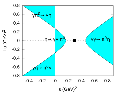
Figure 1: Physical regions for $\gamma\gamma\to\pi\eta$, $\gamma\pi\to\gamma\eta$ scattering and $\eta\to\gamma\gamma\pi^{0}$ decay. The black square indicates the soft pion point.

The polarisation vectors of the two photons $\epsilon_{1}(q_{1},\lambda)$, $\epsilon_{2}(q_{2},\lambda^{\prime})$ in this frame read

$$\epsilon_{1}(q_{1},\lambda)=\frac{1}{\sqrt{2}}\begin{pmatrix}0\\ -\lambda\\ -i\\ 0\\ \end{pmatrix},\quad\epsilon_{2}(q_{2},\lambda^{\prime})=\frac{1}{\sqrt{2}}\begin{pmatrix}0\\ \lambda^{\prime}\\ -i\\ 0\\ \end{pmatrix}$$ (6)

and they satisfy $\epsilon_{1}\cdot q_{1}=\epsilon_{2}\cdot q_{2}=\epsilon_{1}\cdot q_{2}=\epsilon_{2}\cdot q_{1}=0\ .$

2.2 Amplitudes

We denote the $\gamma\gamma\to\eta\pi$ helicity amplitude as $L_{\lambda\lambda^{\prime}}$

$$\mathrel{\hbox{$<$}\kern-3.5pt\lower 5.33708pt\hbox{$\scriptstyle{out}$}}\eta(p_{1})\pi(p_{2})|\gamma(q_{1},\lambda)\gamma(q_{2},\lambda^{\prime})\mathrel{\hbox{$>$}\kern-3.5pt\lower 5.33708pt\hbox{$\scriptstyle{in}$}}=ie^{2}(2\pi)^{4}\delta(P_{f}-P_{i})\,\hbox{e}^{i(\lambda-\lambda^{\prime})\phi}L_{\lambda\lambda^{\prime}}(s,t)$$ (7)

(we have factored out the electric charge $e$ and the dependence on the azimuthal angle $\phi$) while for the $\gamma\gamma\to K\bar{K}$ amplitudes we use the same notation as in previous work: $K^{c}_{\lambda\lambda^{\prime}}(s,t)$ for charged kaons and $K^{n}_{\lambda\lambda^{\prime}}(s,t)$ for neutral kaons. Helicity amplitudes are convenient for performing the partial wave expansion [34]. They can be expressed in terms of tensor amplitudes using the reduction formulas, e.g.

$$\hbox{e}^{i(\lambda-\lambda^{\prime})\phi}L_{\lambda\lambda^{\prime}}(s,t)=\epsilon_{1}^{\mu}(q_{1},\lambda)\epsilon_{2}^{\nu}(q_{2},\lambda^{\prime})W_{\mu\nu}(q_{1},q_{2},p_{1},p_{2})\ .$$ (8)

By gauge invariance, the tensor amplitude $W_{\mu\nu}$ must satisfy the two Ward identities

$$q_{1}^{\mu}W_{\mu\nu}=q_{2}^{\nu}W_{\mu\nu}=0\ .$$ (9)

One can form two independent tensors which satisfy (9) which we take as

$$\begin{array}[]{l}T_{1}^{\mu\nu}=\dfrac{1}{2}sg^{\mu\nu}-q_{1}^{\nu}q_{2}^{\mu}\\[5.69046pt] T_{2}^{\mu\nu}=2s\Delta^{\mu}\Delta^{\nu}+4q_{1}.\Delta\,q_{2}.\Delta\,g^{\mu\nu}-4q_{2}.\Delta\,q_{1}^{\nu}\Delta^{\mu}-4q_{1}.\Delta\,q_{2}^{\mu}\Delta^{\nu}\end{array}$$ (10)

with

$$\Delta=p_{1}-p_{2}\ .$$ (11)

The tensor amplitude $W^{\mu\nu}$ can then be expressed in terms of two scalar amplitudes $A$, $B$

$$W^{\mu\nu}(q_{1},q_{2},p_{1},p_{2})=A(s,t,u)T_{1}^{\mu\nu}+B(s,t,u)T_{2}^{\mu\nu}$$ (12)

which satisfy dispersion relations. Using eqs. (5) (6) one can easily express the helicity amplitudes $L_{\lambda\lambda^{\prime}}$ in terms of the two scalar amplitudes,

$$\begin{array}[]{l}L_{++}=L_{--}=\dfrac{s}{2}\,A(s,t)+s(2m_{1}^{2}+2m_{2}^{2}-s)\,B(s,t)\\[5.69046pt] L_{+-}=L_{-+}=\sin^{2}\theta\lambda_{12}(s)B(s,t)\ .\\ \end{array}$$ (13)

Assuming unpolarised photon beams the differential cross-section reads,

$$\frac{d\sigma^{\gamma\gamma\to M_{1}M_{2}}}{d\cos\theta}=\frac{\pi\alpha^{2}}{4s^{2}}\sqrt{\lambda_{12}(s)}\left(|L_{++}|^{2}+|L_{+-}|^{2}\right)\ .$$ (14)

Concerning the $\eta\to\pi\gamma\gamma$ decay amplitude, the double differential distribution in the Dalitz plot reads,

$$\frac{d^{2}\Gamma^{\eta\to\gamma\gamma\pi}}{dsdt}=\frac{\alpha^{2}}{8\pi m_{\eta}^{3}}\left(|L_{++}|^{2}+|L_{+-}|^{2}\right)\$$ (15)

and the distribution as a function of $s$ only (which is the one available experimentally) is given by

$$\frac{d\Gamma^{\eta\to\gamma\gamma\pi}}{ds}=\frac{\alpha^{2}}{32\pi m_{\eta}^{3}}\sqrt{\lambda_{12}(s)}\int_{-1}^{1}d\cos\theta\left(|L_{++}|^{2}+|L_{+-}|^{2}\right)\ .$$ (16)

2.3 Isospin

Using the following (usual) isospin assignments for the pions and the kaons

$$\begin{pmatrix}{\pi^{+}}\\ {\pi^{0}}\\ {\pi^{-}}\\ \end{pmatrix}\sim\begin{pmatrix}-{|11\rangle}\\ {|10\rangle}\\ {|1,\!-\!1\rangle}\\ \end{pmatrix},\qquad\begin{pmatrix}{K^{+}}\\ {K^{0}}\\ \end{pmatrix}\sim\begin{pmatrix}{|{{1\over 2}{1\over 2}}\rangle}\\[5.69046pt] {|{{1\over 2}{-1\over 2}}\rangle}\\ \end{pmatrix},\qquad\begin{pmatrix}{\bar{K}^{0}}\\ {K^{-}}\\ \end{pmatrix}\sim\begin{pmatrix}{|{{1\over 2}{1\over 2}}\rangle}\\[5.69046pt] -{|{{1\over 2}{-1\over 2}}\rangle}\\ \end{pmatrix}$$ (17)

while $\eta\sim{|0,0\rangle}$, the relations between the amplitudes $\gamma\gamma\to{K^{+}}{K^{-}}$, ${K^{0}}{\bar{K}^{0}}$ and the isospin amplitudes $\gamma\gamma\to(K\bar{K})_{I=0,1}$ read,

$$\left(\begin{array}[]{l}K^{0}_{\lambda\lambda^{\prime}}\\ K^{1}_{\lambda\lambda^{\prime}}\end{array}\right)=\left(\begin{array}[]{rr}-\sqrt{\frac{1}{2}}&-\sqrt{\frac{1}{2}}\\ -\sqrt{\frac{1}{2}}&\sqrt{\frac{1}{2}}\end{array}\right)\left(\begin{array}[]{l}K^{c}_{\lambda\lambda^{\prime}}\\ K^{n}_{\lambda\lambda^{\prime}}\end{array}\right)\ ,$$ (18)

and the analogous relations between the amplitudes $\gamma\gamma\to{\pi^{+}}{\pi^{-}}$, ${\pi^{0}}{\pi^{0}}$ and the corresponding isospin $I=0,2$ amplitudes (which will also be needed) is

$$\left(\begin{array}[]{l}H^{0}_{\lambda\lambda^{\prime}}\\ H^{2}_{\lambda\lambda^{\prime}}\end{array}\right)=\left(\begin{array}[]{rr}-\sqrt{\frac{2}{3}}&-\sqrt{\frac{1}{3}}\\ -\sqrt{\frac{1}{3}}&\sqrt{\frac{2}{3}}\end{array}\right)\left(\begin{array}[]{r}\sqrt{2}\,H^{c}_{\lambda\lambda^{\prime}}\\ H^{n}_{\lambda\lambda^{\prime}}\end{array}\right)\ .$$ (19)

3 Partial waves: unitarity, analyticity

3.1 Right-hand cut and unitarity relations

It is convenient to collect the three $I=1$ scattering amplitudes $\pi\eta\to\pi\eta$, $\pi\eta\to K\bar{K}$ and $K\bar{K}\to K\bar{K}$ into a $2\times 2$ matrix

$$\bm{T}\equiv\begin{pmatrix}T^{\pi\eta\to\pi\eta}&T^{\pi\eta\to K\bar{K}}\\ T^{\pi\eta\to K\bar{K}}&T^{K\bar{K}\to K\bar{K}}\\ \end{pmatrix}$$ (20)

and we can define the partial wave expansions as

$$\bm{T}(s,t,u)=16\pi\sum(2j+1)\bm{T}_{j}(s)P_{j}(\cos\theta)$$ (21)

where $\theta$ is the scattering angle in the centre-of-mass system. The unitarity relation for the partial waves are easily derived and reads

$${\rm Im\,}[\bm{T}_{j}(s)]=\bm{T}_{j}(s)\bm{\Sigma(s)}\bm{T}^{*}_{j}(s)$$ (22)

with

$$\bm{\Sigma(s)}=\begin{pmatrix}\dfrac{\sqrt{\lambda_{\pi\eta}(s)}}{s}\,\theta(s-(m_{\pi}+m_{\eta})^{2})&0\\ 0&\sqrt{\dfrac{s-4m_{K}^{2}}{s}}\,\theta(s-4m_{K}^{2})\\ \end{pmatrix}\ .$$ (23)

Concerning the $I=1$ photon-photon amplitudes we define the partial-wave expansion as

$$\left(\begin{array}[]{l}L_{\lambda\lambda^{\prime}}(s,t)\\ K^{1}_{\lambda\lambda^{\prime}}(s,t)\end{array}\right)=\sum_{j}(2j+1)\left(\begin{array}[]{l}l_{j,\lambda\lambda^{\prime}}(s)\\ k^{1}_{j,\lambda\lambda^{\prime}}(s)\end{array}\right)\,d^{j}_{\lambda-\lambda^{\prime},0}(\theta)\ .$$ (24)

The unitarity relations for the $S$-waves, as will be implemented below, read

$${\rm Im\,}\begin{pmatrix}l_{0++}(s)\\[8.5359pt] k^{1}_{0++}(s)\\ \end{pmatrix}=\bm{T}^{*}_{j}(s)\bm{\Sigma(s)}\begin{pmatrix}l_{0++}(s)\\[8.5359pt] k^{1}_{0++}(s)\\ \end{pmatrix}\ ,$$ (25)

which also give the discontinuities of the partial-waves (extended to complex values of $s$) across the right-hand cut.

3.2 $\pi\pi$ (isospin violating) contribution in $S$-wave unitarity

The unitarity relation written above (25) collects the contributions from the $\pi\eta$ and the $K\bar{K}$ states. Let us also consider the contribution from the $\pi^{+}\pi^{-}$ state, which has the form

$${\rm Im\,}[{\langle\pi^{0}\eta|{\cal T}|\gamma\gamma\rangle}]_{\pi\pi}=\frac{1}{2}\int d\Phi(p_{+},p_{-})\,{\langle\pi^{0}\eta|{\cal T}|{\pi^{+}}{\pi^{-}}\rangle}{\langle{\pi^{+}}{\pi^{-}}|{\cal T}^{\dagger}|\gamma\gamma\rangle}$$ (26)

where $d\Phi$ is the phase-space integration measure. This contribution, being proportional to the $\pi\pi\to\eta\pi$ amplitude, is isospin violating but it is enhanced at low energy due the large size of the $\gamma\gamma\to\pi^{+}\pi^{-}$ amplitude [33]. The ChPT evaluation performed in ref. [33] amounts to using the $O(p^{2})$ tree-level amplitudes for both $\pi\pi\to\eta\pi$ and $\gamma\gamma\to\pi^{+}\pi^{-}$ in eq. (26). An evaluation which goes beyond the chiral expansion can be performed which we now discuss.

We consider only the $S$-wave contribution in eq. (26) and a restricted kinematical region such that $s,t,u<1$ $\hbox{GeV}^{2}$. In such a region, the ${\pi^{+}}{\pi^{-}}\to\eta{\pi^{0}}$ amplitude can be approximated in terms of three one-variable functions $M_{0}$, $M_{1}$, $M_{2}$ (see [35, 36]),

$$\begin{array}[]{l}T^{{\pi^{+}}{\pi^{-}}\to\eta{\pi^{0}}}(s,t,u)=\\[5.69046pt] \qquad-\epsilon_{L}\big{[}M_{0}(s)-\frac{2}{3}M_{2}(s)+(s-u)M_{1}(t)+(s-t)M_{1}(u)+M_{2}(t)+M_{2}(u)\big{]}\ .\end{array}$$ (27)

An isospin violating parameter $\epsilon_{L}$ has been factorised which may be taken as [37]

$$\epsilon_{L}=\dfrac{\left({m}^{2}_{K^{0}}-{m}^{2}_{K^{+}}\right)_{QCD}}{3\sqrt{3}F_{\pi}^{2}}\ .$$ (28)

The three $M_{I}$ functions obey a set of coupled Khuri-Treiman integral equations., see ref. [37] for a complete review of work on this subject. We will use here the evaluation of the ${K^{0}}-{K^{+}}$ QCD mass difference from ref. [38] (updated in [37]) based on experimental data on $\eta\to 3\pi$ decays: $\left({m}^{2}_{K^{0}}-{m}^{2}_{K^{+}}\right)_{QCD}=(6.24\pm 0.38)\cdot 10^{-3}$ GeV², which gives

$$\epsilon_{L}=0.141\pm 0.009\ .$$ (29)

The amplitudes corresponding to a given $\pi\pi$ isospin state $I,I_{z}$

$${\cal M}^{I\,I_{z}}\equiv{\langle\eta\pi|T|\pi\pi;I\,I_{z}\rangle}$$ (30)

are easily expressed using crossing symmetry and the Wigner-Eckart theorem. In the unitarity relation (26) the amplitudes with $I=0,2$, ${\cal M}^{00}$ and ${\cal M}^{20}$, are needed which have the following expressions

$$\begin{array}[]{l@{}r@{}l}{\cal M}^{00}(s,t,u)=&\sqrt{3}\,\epsilon_{L}&\left[M_{0}(s)+{1\over 3}M_{0}(t)+{10\over 9}M_{2}(t)+{2\over 3}(s-u)M_{1}(t)+(t\leftrightarrow u)\right]\\[5.69046pt] {\cal M}^{20}(s,t,u)=&-\frac{2\sqrt{6}}{3}\,\epsilon_{L}&\left[M_{2}(s)+{1\over 2}M_{0}(t)+{1\over 6}M_{2}(t)-{1\over 2}(s-u)M_{1}(t)+(t\leftrightarrow u)\right]\\ \end{array}$$ (31)

in terms of the $M_{I}$ functions. We denote the angular integrals of these amplitudes as

$$\begin{array}[]{l}\frac{1}{2}\displaystyle\int_{-1}^{1}dz\,{\cal M}^{00}(s,t,u)\equiv\sqrt{3}\,\epsilon_{L}\left(M_{0}(s)+\hat{M}_{0}(s)\right)\\[5.69046pt] \frac{1}{2}\displaystyle\int_{-1}^{1}dz\,{\cal M}^{20}(s,t,u)\equiv-\frac{2\sqrt{6}}{3}\,\epsilon_{L}\left(M_{2}(s)+\hat{M}_{2}(s)\right)\ .\end{array}$$ (32)

With this notation, the $\pi\pi$ contribution to the unitarity relation is finally expressed as follows,

$$\begin{array}[]{l@{}l}{\rm disc\,}[{l}_{0,++}(s)]_{\pi\pi}=\epsilon_{L}\dfrac{\sqrt{3}}{32\pi}\sqrt{\dfrac{s-4m_{\pi}^{2}}{s}}\,\bigg{[}&\left(h^{0}_{0,++}(s)\right)^{*}(M_{0}(s)+\hat{M}_{0}(s))\\[5.69046pt] &-\frac{2\sqrt{2}}{3}\left(h^{2}_{0,++}(s)\right)^{*}(M_{2}(s)+\hat{M}_{2}(s))\bigg{]}\\ \end{array}$$ (33)

where

$${\rm disc\,}[{l}_{0,++}(s)]_{\pi\pi}\equiv\frac{{l}_{0,++}(s+i\epsilon)-{l}_{0,++}(s-i\epsilon)}{2i}\ ,$$ (34)

and $h^{I}_{0,++}(s)$ are the two $S$-wave $\gamma\gamma\to(\pi\pi)^{I}$ amplitudes with $I=0,2$. This $\pi\pi$ discontinuity of ${l}_{0++}$ can be estimated from eq. (33) using inputs from ref. [28] for $\gamma\gamma\to\pi\pi$ and from  [27] for $\pi\pi\to\eta\pi$. The result of this estimate is illustrated on fig. 2 and compared with the chiral calculation at NLO. The dispersive evaluation displays a square-root singularity at $s=(m_{\eta}-m_{\pi})^{2}$ induced by the endpoint of the left-hand cut in the functions $\hat{M}_{0}$, $\hat{M}_{2}$ which overlaps with the right-hand cut as a result of the instability of the $\eta$. As a further consequence, the phase of the partial-waves $M_{I}+\hat{M}_{I}$ violate Watson’s theorem and do not cancel with the phases of $h_{0,++}^{I}$ such that the discontinuity has both a real and an imaginary part.

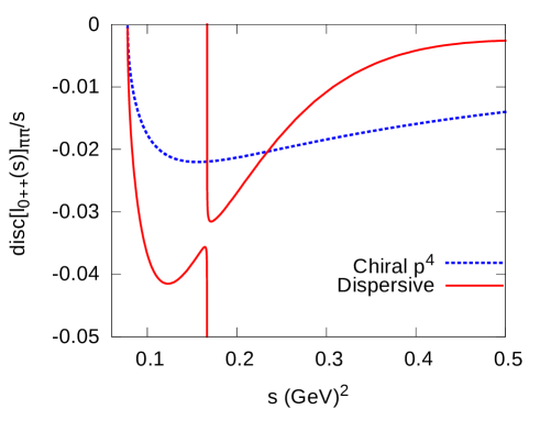
Figure 2: Discontinuity of the $\gamma\gamma\to\pi\eta$ $S$-wave amplitude (real part) across the ${\pi^{+}}{\pi^{-}}$ cut computed using dispersive results for the $\gamma\gamma\to\pi\pi$ and $\pi\pi\to\eta\pi$ amplitudes, compared to the chiral $O(p^{4})$ result.

3.3 Left-hand cut: Born amplitudes

A left hand cut in the $\gamma\gamma$ partial-waves is generated by singularities in the cross-channels $\gamma P_{1}\to\gamma P_{2}$. In the case when $P_{1}=P_{2}={K^{+}}$ or ${\pi^{+}}$ the leading singularity is the kaon or pion pole and the corresponding (so-called Born) amplitudes read

$$\begin{array}[]{l}A_{P}^{Born}(s,t,u)=\dfrac{s}{(t-m^{2}_{P})(u-m^{2}_{P})}\\[8.5359pt] B_{P}^{Born}(s,t,u)=\dfrac{1}{2(t-m^{2}_{P})(u-m^{2}_{P})}\\ \end{array}$$ (35)

with $P={K^{+}},\ {\pi^{+}}$. We will need the $I=1$ component of the $K^{+}$ Born amplitude projected on the $S$-wave which reads,

$$k^{1,Born}_{0,++}(s)=-\frac{2\sqrt{2}\,m^{2}_{{K^{+}}}}{s}\,L_{K^{+}}(s),\quad L_{K^{+}}(s)=\frac{1}{\beta_{{K^{+}}}(s)}\log\frac{1+\beta_{{K^{+}}}(s)}{1-\beta_{{K^{+}}}(s)}$$ (36)

with $\beta_{P}(s)=\sqrt{1-4m^{2}_{P}/s}$. We also recall the expressions of the $J=2$ Born helicity amplitudes

$$\begin{array}[]{ll}k^{1,Born}_{2++}(s)=&-\dfrac{2m^{2}_{K^{+}}}{s\,\beta^{2}_{K^{+}}(s)}\left[(\beta^{2}_{K^{+}}(s)-3)\,L_{K^{+}}(s)+6\right]\\[11.38092pt] k^{1,Born}_{2+-}(s)=&\dfrac{\sqrt{6}}{4s\beta^{2}_{K^{+}}(s)}\left[(1-\beta^{2}_{K^{+}}(s))^{2}\,L_{K^{+}}(s)+\dfrac{10}{3}\beta^{2}_{K^{+}}(s)-2\right]\ .\end{array}$$ (37)

3.4 Left-hand cut: vector meson exchanges

Leading contributions to the left-hand cut in the ${\pi^{0}}\eta$ amplitudes are modelled from the $\rho$, $\omega$, $\phi$ vector meson exchanges. We define the $VP\gamma$ coupling constants $G_{VP}$ through simple Lagrangians

$${\cal L}_{VP\gamma}=eG_{VP}\,\epsilon^{\mu\nu\alpha\beta}F_{\mu\nu}\partial_{\alpha}{P}V_{\beta}$$ (38)

from which one can relate their values to the decay widths of the vector mesons via

$$\Gamma_{V\to P\gamma}=\alpha C^{2}_{VP}\frac{(m_{V}^{2}-m_{P}^{2})^{3}}{6m_{V}^{3}}\ .$$ (39)

The vector-exchange contributions to the $\gamma\gamma\to P_{1}P_{2}$ amplitudes are easily computed,

$$\begin{array}[]{l}A_{V}^{P_{1}P_{2}}(s,t,u)=G_{VP_{1}}G_{VP_{2}}\dfrac{-4t-2m_{1}^{2}-2m_{2}^{2}+s}{2(m_{V}^{2}-t)}+(t\leftrightarrow u)\\[7.11317pt] B_{V}^{P_{1}P_{2}}(s,t,u)=G_{VP_{1}}G_{VP_{2}}\dfrac{1}{4(m_{V}^{2}-t)}+(t\leftrightarrow u)\ .\\ \end{array}$$ (40)

They give rise to poles in the zero-width approximation, which is adequate in the kinematical regions of interest here. The helicity amplitudes are

$$\begin{array}[]{l}L_{V,++}^{P_{1}P_{2}}(s,\theta)=C_{VP_{1}}C_{VP_{2}}\dfrac{-st}{m_{V}^{2}-t}+(t\leftrightarrow u)\\[8.5359pt] L_{V,+-}^{P_{1}P_{2}}(s,\theta)=C_{VP_{1}}C_{VP_{2}}\dfrac{\sin^{2}\theta\lambda_{12}(s)}{4(m_{V}^{2}-t)}+(t\leftrightarrow u)\\ \end{array}$$ (41)

and the corresponding partial-waves with $J=0,2$ have the following form

$$\begin{array}[]{ll}l^{V}_{0,++}(s)=&C_{V\pi}C_{V\eta}\,2s\left(1-m_{V}^{2}L_{V}(s)\right)\\[2.84544pt] l^{V}_{2,++}(s)=&C_{V\pi}C_{V\eta}\,m_{V}^{2}s\,\Big{\{}(1-3X_{V}^{2}(s))L_{V}(s)+\dfrac{6X_{V}(s)}{\sqrt{\lambda_{12}(s)}}\Big{\}}\\[8.5359pt] l^{V}_{2,+-}(s)=&\frac{\sqrt{6}}{8}C_{V\pi}C_{V\eta}\,\Big{\{}\lambda_{12}(s)(1-X_{V}^{2}(s))^{2}\,L_{V}(s)\\[5.69046pt] &\quad-\frac{2}{3}\sqrt{\lambda_{12}(s)}X_{V}(s)(3X_{V}^{2}(s)-5)\Big{\}}\end{array}$$ (42)

with

$$X_{V}(s)=\frac{s-m_{1}^{2}-m_{2}^{2}+2m_{V}^{2}}{\sqrt{\lambda_{12}(s)}}\$$ (43)

which is the cosine of the scattering angle when $t=m_{V}^{2}$. The function $L_{V}(s)$ is given by the angular integral

$$L_{V}(s)=\int_{-1}^{1}dz\,\frac{s+2m_{V}^{2}-m_{1}^{2}-m_{2}^{2}}{\lambda_{12}(s)(1-z^{2})+4m_{V}^{2}(s-s_{V})}$$ (44)

with

$$s_{V}=-\frac{(m_{V}^{2}-m_{1}^{2})(m_{V}^{2}-m_{2}^{2})}{m_{V}^{2}}\ ,$$ (45)

it can be expressed in terms of $X_{V}$ as

$$L_{V}(s)=\frac{\log(X_{V}(s)+1)-\log(X_{V}(s)-1)}{\sqrt{\lambda_{12}(s)}}\ .$$ (46)

We note that the partial-wave $l^{V}_{0++}(s)$ has a soft pion Adler zero at $s=s_{A}$ which can be approximated as

$$s_{A}=m_{\eta}^{2}+m_{\pi}^{2}\left(1+\frac{m_{\eta}^{2}}{m_{V}^{2}}\left(-\frac{2}{3}+\frac{4}{135}\frac{m_{\pi}^{2}m_{\eta}^{2}}{m_{V}^{4}}-\frac{8}{8505}\frac{m_{\pi}^{4}m_{\eta}^{4}}{m_{V}^{8}}+\cdots\right)\right)\ .$$ (47)

From the integral representation (44) one sees that the function $L_{V}$ has endpoint singularities at $z=\pm 1$ when $s=s_{V}$, which thus corresponds to a branch point of $L_{V}(s)$. Another endpoint singularity occurs when $s=\infty$. When $s>s_{V}$, the denominator remains strictly positive. Therefore, $L_{V}$ is an analytic function of $s$ with a cut on the negative real axis: $-\infty<s<s_{V}$. The discontinuity of $L_{V}$ along the cut is easily determined

$${\rm Im\,}[L_{V}(s+i\epsilon)]=-\frac{\pi}{\sqrt{\lambda_{12}(s)}}\theta(s_{V}-s)$$ (48)

from which one deduces the left-cut discontinuities of the vector-exchange partial-waves

$$\begin{array}[]{ll}\dfrac{1}{\pi}{\rm Im\,}[l^{V}_{0,++}(s)]=&2C_{V\pi}C_{V\eta}\,\dfrac{s\,m_{V}^{2}}{\sqrt{\lambda_{12}(s)}}\,\theta(s_{V}-s)\\[11.38092pt] \dfrac{1}{\pi}{\rm Im\,}[l^{V}_{2,++}(s)]=&C_{V\pi}C_{V\eta}\,\dfrac{s\,m_{V}^{2}}{\sqrt{\lambda_{12}(s)}}(3X_{V}^{2}(s)-1)\,\theta(s_{V}-s)\\[11.38092pt] \dfrac{1}{\pi}{\rm Im\,}[l^{V}_{2,+-}(s)]=&-\dfrac{\sqrt{6}}{8}C_{V\pi}C_{V\eta}\,\sqrt{\lambda_{12}(s)}\,{(1-X_{V}^{2}(s))^{2}}\theta(s_{V}-s)\ .\end{array}$$ (49)

We will use these discontinuities in the Muskhelishvili-Omnès representations below. We must consider also the vector exchange contributions for the $\gamma\gamma\to(K\bar{K})_{I=1}$ amplitudes, we denote the relevant combination of coupling constants as

$$\tilde{C}_{K^{*}}^{(1)}\equiv\frac{1}{\sqrt{2}}\left(-C^{2}_{K^{*}K^{+}}+C^{2}_{K^{*}K^{0}}\right)\ .$$ (50)

The imaginary parts of the $J=0,2$ partial-wave amplitudes along the left-hand cut read

$$\begin{array}[]{ll}\dfrac{1}{\pi}{\rm Im\,}[k^{V}_{0,++}(s)]=&2\tilde{C}_{K^{*}}^{(1)}\,\dfrac{s\,m_{K^{*}}^{2}}{\sqrt{\lambda_{KK}(s)}}\theta(s_{K^{*}}-s)\\[11.38092pt] \dfrac{1}{\pi}{\rm Im\,}[k^{V}_{2,++}(s)]=&\,\tilde{C}_{K^{*}}^{(1)}\dfrac{s\,m_{K^{*}}^{2}}{\sqrt{\lambda_{KK}(s)}}(3X_{K^{*}}^{2}(s)-1)\,\theta(s_{K^{*}}-s)\\[11.38092pt] \dfrac{1}{\pi}{\rm Im\,}[k^{V}_{2,+-}(s)]=&-\dfrac{\sqrt{6}}{8}\tilde{C}_{K^{*}}^{(1)}\,\sqrt{\lambda_{KK}(s)}\,{(1-X_{K^{*}}^{2}(s))^{2}}\theta(s_{K^{*}}-s)\ .\end{array}$$ (51)

The updated values of the couplings $C_{VP}$ are collected in table 1 below.

	$\Gamma$ (keV)	$C_{VP}$(GeV-1)
$\rho^{0}\rightarrow\pi^{0}\gamma$	$69(9)$	$0.368(24)$
$\rho^{0}\rightarrow\eta\gamma$	$44(3)$	$0.789(30)$
$\omega\rightarrow\pi^{0}\gamma$	$713(26)$	$1.160(20)$
$\omega\rightarrow\eta\gamma$	$3.8(4)$	$0.222(11)$
$\phi\rightarrow\pi^{0}\gamma$	$5.5(2)$	$0.067(1)$
$\phi\rightarrow\eta\gamma$	$55(1)$	$0.345(4)$
$K^{*\pm}\rightarrow K^{\pm}\gamma$	$50(5)$	$0.418(22)$
$K^{*0}\rightarrow K^{0}\gamma$	$116(11)$	$-0.636(30)$

Table 1: Radiative widths of vector mesons and corresponding coupling constants. The relative signs of the couplings are determined assuming flavour symmetry.

4 Representations of the $J=0,2$ partial-waves

4.1 Muskhelishvili-Omnès representations for the $S$-waves

In order to write a dispersive representation for $l_{0++}$ some knowledge concerning its asymptotic behaviour is needed. Let us then consider the angular integral,

$$l_{0++}(s)\equiv\int_{0}^{1}dz\,L_{++}(s,t)\$$ (52)

in the $s\to\infty$ limit. There are two regions of the angular variable $z$ for which the behaviour of the integrand is known: a) when $z$ is close to 0, then $t\sim u\sim-s\sim-\infty$. In this regime, $L_{++}(s,t)$ can be estimated from QCD-based methods [39, 40] according to which one has

$$L_{++}(s,t)<<L_{+-}(s,t)\sim\frac{\alpha_{s}(s)}{s}\ .$$ (53)

b) When $z$ is close to 1, then $|t|<<s$ which is the region where Regge theory applies, the leading contribution from the vector meson trajectory gives

$$L_{++}(s,t)\sim\beta_{V}(t)(\alpha^{\prime}s)^{\alpha_{V}+\alpha^{\prime}t}$$ (54)

with $\alpha_{V}\simeq 0.5$, $\alpha^{\prime}\simeq 0.9$ $\hbox{GeV}^{-1}$ and $\beta_{V}(t)$ is a smooth function when $t<0$. Assuming only that the integrand evolves smoothly between these two regimes when $0\leq z\leq 1$, one deduces that the $l_{0++}(s)$ should not grow faster than $\sqrt{s}$ when $s\to\infty$.

Furthermore, the $J=0$ partial-waves obey soft-photon theorems  [7, 8] which imply that the ratios $l_{0++}(s)/s$ and $(k^{1}_{0++}(s)-k^{1,Born}_{0++}(s))/s$ remain finite when $s\to 0$. Therefore, they can be expressed as unsubtracted dispersion relations in terms of the left-hand and right-hand cuts discontinuities,

$$\begin{array}[]{l}l_{0++}(s)=s\left[\dfrac{1}{\pi}{\displaystyle\int_{-\infty}^{{{s}_{V}}}}ds^{\prime}\,\dfrac{{\rm Im\,}[l_{0++}(s^{\prime})]}{s^{\prime}(s^{\prime}-s)}+\dfrac{1}{\pi}{\displaystyle\int_{m_{+}^{2}}^{\infty}}ds^{\prime}\,\dfrac{{\rm Im\,}[l_{0++}(s^{\prime})]}{s^{\prime}(s^{\prime}-s)}\right]\\[11.38092pt] k^{1}_{0++}(s)=k_{0++}^{1,Born}(s)+s\left[\dfrac{1}{\pi}{\displaystyle\int_{-\infty}^{{s_{K^{*}}}}}ds^{\prime}\,\dfrac{{\rm Im\,}[k^{1}_{0++}(s^{\prime})]}{s^{\prime}(s^{\prime}-s)}+\dfrac{1}{\pi}{\displaystyle\int_{m_{+}^{2}}^{\infty}}ds^{\prime}\,\dfrac{{\rm Im\,}[k^{1}_{0++}(s^{\prime})]}{s^{\prime}(s^{\prime}-s)}\right]\end{array}$$ (55)

with $m_{+}=m_{\pi}+m_{\eta}$. The isospin symmetry limit has been assumed here, implying that the $\eta$ meson is stable and the discontinuities are real. At low energies the left-cut discontinuities are dominated by the vector meson exchanges. We will introduce subtractions, in order to reduce the influence of the higher energy regions where the discontinuities are not known. The right-cut discontinuities are given by the unitarity relations. Unitarity is known to be saturated with two channels to a very good approximation in the region of the $a_{0}(980)$ resonance. We will assume that elastic unitarity holds below the $K\bar{K}$ threshold and that two-channel unitarity remains a sufficiently good approximation up to $\sqrt{s}=1.4$ GeV. Under the assumption of two-channel unitarity the dispersion relations (55) form a set of coupled inhomogeneous Muskhelishvili equations. They can be solved in terms of a two-channel MO matrix which satisfies a homogeneous set of coupled equations in terms of the $T$ matrix

$$\bm{\Omega}_{0}(s)=\dfrac{1}{\pi}\int_{m_{+}^{2}}^{\infty}\frac{ds^{\prime}}{s^{\prime}-s}\bm{T}(s)\bm{\Sigma}(s)\bm{\Omega}^{*}_{0}(s)\$$ (56)

Asymptotic conditions on the phase-shifts are imposed which ensure that the set of equations (56) has a unique solution once initial conditions at $s=0$ are given (see sec. 3.2 in ref. [27] and references therein). At $s=0$ one can take

$$\bm{\Omega}_{0}(0)=\begin{pmatrix}1&0\\ 0&1\\ \end{pmatrix}\ .$$ (57)

Multiplying the amplitudes $(l_{0++},k_{0++})$ by the inverse of the matrix $\bm{\Omega}_{0}$ removes the right-hand cuts. We can use this property in writing once-subtracted dispersion relations for the two functions

$$\begin{pmatrix}\phi_{1}(s)\\ \phi_{2}(s)\\ \end{pmatrix}\equiv\bm{\Omega}_{0}^{-1}(s)\begin{pmatrix}l_{0++}(s)/s\\[8.5359pt] (k^{1}_{0++}(s)-k_{0++}^{1,Born}(s))/s\\ \end{pmatrix}\ .$$ (58)

This provides MO-type dispersive representations for the $\gamma\gamma$ amplitudes $l_{0++}(s)$, $k_{0++}(s)$ in terms of their imaginary parts on the left-cut and two parameters, $b_{l}$, $b_{k}$

$$\begin{pmatrix}l_{0++}(s)\\ k^{1}_{0++}(s)\\ \end{pmatrix}=\begin{pmatrix}0\\ k_{0++}^{1,Born}(s)\\ \end{pmatrix}+s\,\bm{\Omega}_{0}(s)\begin{pmatrix}b_{l}+L_{1}(s)+R_{1}(s)\\ b_{k}+L_{2}(s)+R_{2}(s)\\ \end{pmatrix}\ .$$ (59)

The functions $L_{i}(s)$ are dispersive integrals over the left-hand cuts. We express them in a way which allows to easily implement the presence of an Adler zero at $s=s_{A}$ in the amplitude $l_{0++}$ (see appendix B)

$$\begin{array}[]{ll}L_{i}(s)=&\dfrac{s-s_{A}}{\pi}{\displaystyle\int_{-\infty}^{{s}_{V}}}\dfrac{ds^{\prime}}{s^{\prime}(s^{\prime}-s_{A})(s^{\prime}-s)}\,D_{i1}(s^{\prime})\,{\rm Im\,}[l^{V}_{0++}(s^{\prime})]\\[11.38092pt] &+\dfrac{s-s_{A}}{\pi}{\displaystyle\int_{-\infty}^{s_{K^{*}}}}\dfrac{ds^{\prime}}{s^{\prime}(s^{\prime}-s_{A})(s^{\prime}-s)}\,D_{i2}(s^{\prime})\,{\rm Im\,}[k^{V}_{0++}(s^{\prime})]\end{array}$$ (60)

where the functions $D_{ij}(s)$ are the matrix elements of the inverse of the Omnès matrix,

$$\bm{D}(s)\equiv\bm{\Omega}_{0}^{-1}(s)\ .$$ (61)

The functions $R_{i}(s)$, secondly, are the dispersive integrals over the right-hand cut,

$$R_{i}(s)=-\frac{s-s_{A}}{\pi}\int_{4m_{K}^{2}}^{\infty}\frac{ds^{\prime}}{s^{\prime}(s^{\prime}-s_{A})(s^{\prime}-s)}\,{\rm Im\,}[D_{i2}(s^{\prime})]\,k_{0++}^{1,Born}(s^{\prime})\ .$$ (62)

A relation between the parameters $b_{l}$ and $b_{k}$ can be derived from imposing that the amplitude $l_{0++}$ has an Adler zero at $s=s_{A}$,

$$b_{l}=-b_{k}\Omega_{12}(s_{A})/\Omega_{11}(s_{A})\ .$$ (63)

The parameter $b_{k}$ will eventually be fitted to the experimental data but we can estimate its order of magnitude by matching the amplitude $k^{1}_{0++}$ with the $SU(3)$ chiral expansion. Including the order $p^{4}$ contributions (see appendixB) and an estimate of the order $p^{6}$ from the vector-meson exchange amplitudes, we obtain

$$\begin{array}[]{ll}b_{k}+L_{2}(0)+R_{2}(0)&\simeq-\dfrac{2\sqrt{2}}{F_{\pi}^{2}}(L_{9}+L_{10})-\sqrt{2}(G^{2}_{K^{*0}K}-G^{2}_{K^{*+}K})\dfrac{m_{K}^{2}}{m_{K^{*}}^{2}}\\[8.5359pt] &\simeq-(0.57\pm 0.03)\ \hbox{GeV}^{-2}\end{array}$$ (64)

using the determination $L_{9}+L_{10}=(1.44\pm 0.08)\cdot 10^{-3}$ taken from ref [41]. Below, the value of $b_{k}$ will be fitted to the experimental data, the resulting combination $b_{k}+L_{2}(0)+R_{2}(0)$ turns out to have a sign compatible with (64) and a magnitude smaller by a factor of two. The result of the dispersive construction of the $S$-wave amplitude $l_{0++}$ is illustrated in fig. 3. The corresponding result for the $K\bar{K}$ amplitude $k^{1}_{0++}$ is shown in appendix C (see fig. 13).

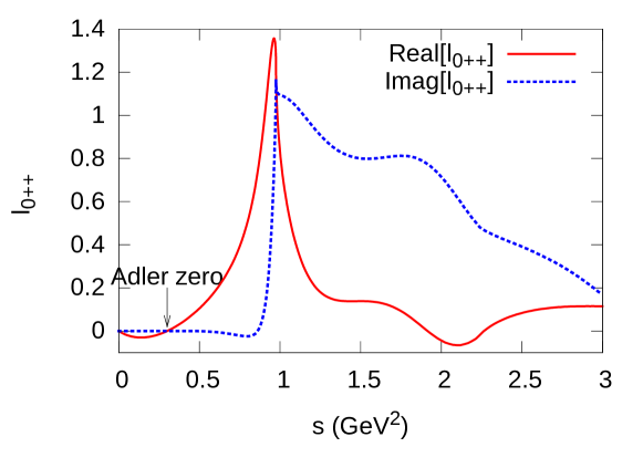
Figure 3: The $S$-wave amplitude $l_{0++}$ from the dispersive construction using the central values of the fitted parameters.

4.2 Dispersive construction of the isospin-violating $S$-wave

In sec. 3.2 we have considered the unitarity contribution to the $\gamma\gamma\to\pi\eta$ $S$-wave amplitude induced by the ${\pi^{+}}{\pi^{-}}$ intermediate state, which is isospin violating. Let us call $\tilde{L}_{++}$ the isospin-violating part of the $\gamma\gamma\to\pi\eta$ helicity amplitude and $\tilde{l}_{0++}$ the corresponding $S$-wave. $\tilde{L}_{++}$ can be defined as a matrix element,

$$\tilde{L}_{++}\equiv{\langle{\pi^{0}}(p_{1})\eta(p_{2})|\frac{1}{2}(m_{d}-m_{u})(\bar{u}u-\bar{d}{d})|\gamma(q_{1},+)\gamma(q_{2},+)\rangle}\ .$$ (65)

We will attempt here to estimate the amplitude $\tilde{l}_{0++}$ at low energy only and we write a dispersive representation keeping only the contribution from the $\pi\pi$ cut,

$${\tilde{l}_{0,++}(s)}\equiv{s}\Big{(}\tilde{\lambda}+\dfrac{s-s_{A}}{\pi}{\displaystyle\int_{4m_{\pi}^{2}}^{\infty}}\dfrac{ds^{\prime}}{s^{\prime}(s^{\prime}-s_{A})(s^{\prime}-s)}\,{\rm disc\,}[{l}_{0,++}(s^{\prime})]_{\pi\pi}\Big{)}\ .$$ (66)

We have used two subtractions in eq. (66) in order to strongly reduce the influence of the energy region above 1 GeV. One subtraction constant is fixed from imposing the soft photon zero. We can then estimate the parameter $\tilde{\lambda}$ in eq. (66) by using the soft pion limit. This limit provides a relation between the amplitude $\tilde{l}_{0++}(s=s_{A})$ and a matrix element of the pseudo-scalar operator $p_{0}=i(\bar{u}\gamma^{5}u+\bar{d}\gamma^{5}d)$ which, in turn, can be estimated using ChPT. This is detailed in appendix B.3. Using eqs. (128) ,(129) from this appendix we obtain the following result for $\tilde{\lambda}$

$$\tilde{\lambda}=\dfrac{3\epsilon_{L}}{8\pi^{2}s_{A}}\,\big{(}1-\dfrac{m_{\pi}^{2}}{3F_{\pi}^{2}}\big{)}\,\big{(}G_{\pi}(s_{A})-\frac{1}{2}G_{K}(s_{A})\big{)}\$$ (67)

where the loop functions $G_{\pi}$, $G_{K}$ are given in eq. (107). The discontinuity ${\rm disc\,}[{l}_{0++}(s)]_{\pi\pi}$ (given in eq. (33)) has a singularity at the pseudo-threshold $s=(m_{\eta}-m_{\pi})^{2}$ induced by the $\pi\pi\to\eta\pi$ partial-wave (see fig. 2). The integral in eq. (66), however, is finite. It is defined by using the $m_{\eta}^{2}+i\epsilon$ limiting prescription exactly in the same way as those which appear in the Khuri-Treiman equations for the $\eta\to 3\pi$ amplitude (see e.g. [35, 42]).

The result, in the low energy region relevant for $\eta\to\pi\gamma\gamma$ is shown in fig. 4 and compared to the corresponding chiral $O(p^{4})$ result from eq. (112). The chiral and dispersive real parts agree at $s=m_{\eta}^{2}$, as a result of the soft pion relation, but the two amplitudes differ substantially at lower energy:

• The cusp at the $\pi\pi$ threshold is much more pronounced in the dispersive amplitude which is approximately five times larger in magnitude than the $p^{4}$ amplitude at $s=4m_{\pi}^{2}$.

• The $p^{4}$ amplitude has a zero at $s=4/3m_{\pi}^{2}$ in contrast to the dispersive amplitude which has no zero in this region. This is because this zero is unrelated to a soft photon constraint and is an accidental feature of the $p^{4}$ amplitude.

Figure 4: Dispersive calculation of the isospin-violating component of the $\eta\to\pi\gamma\gamma$ $S$-wave amplitude (divided by $s$), compared to the chiral result at order $p^{4}$. The shaded area shows the physical region.

4.3 $D$-wave amplitudes modelling:

For the $J=2$ partial-waves one can write unsubtracted dispersion representations analogous to those for $J=0$, e.g.,

$$\begin{array}[]{l@{}l}l_{2\lambda\lambda^{\prime}}(s)=s^{|\lambda+\lambda^{\prime}|/2}\lambda_{12}(s)&\Big{[}\dfrac{1}{\pi}{\displaystyle\int_{-\infty}^{{{s}_{V}}}}ds^{\prime}\,\dfrac{{\rm Im\,}[l_{2\lambda\lambda^{\prime}}(s^{\prime})]}{(s^{\prime})^{|\lambda+\lambda^{\prime}|/2}\lambda_{12}(s^{\prime})(s^{\prime}-s)}\\[14.22636pt] &\qquad+\dfrac{1}{\pi}{\displaystyle\int_{m_{+}^{2}}^{\infty}}ds^{\prime}\,\dfrac{{\rm Im\,}[l_{2\lambda\lambda^{\prime}}(s^{\prime})]}{(s^{\prime})^{|\lambda+\lambda^{\prime}|/2}\lambda_{12}(s^{\prime})(s^{\prime}-s)}\Big{]}\\ \end{array}$$ (68)

displaying the kinematical zeros at $s=m_{\pm}^{2}$ and $s=0$. In the case of $J=2$, however, it seems difficult to derive useful constraints from unitarity as in the case of $J=0$ because in the important energy region of the $a_{2}(1320)$ resonance there are too many contributing channels. We will therefore content with a simple Breit-Wigner estimate of the right-hand cut integral in eq. (68).

We parametrise the coupling of the $a_{2}$ resonance to the $\eta\pi$ channel by a constant $C^{a_{2}}_{\eta\pi}$ defined from the Lagrangian

$${\cal L}_{a_{2}\eta\pi}=C^{a_{2}}_{\eta\pi}\,T_{\mu\nu}(x)\partial^{\mu}\eta(x)\partial^{\nu}\pi^{0}(x)\ .$$ (69)

The couplings to the $\gamma\gamma$ channel involve two constants

$${\cal L}_{T\gamma\gamma}=e^{2}\,T_{\mu\nu}(x)\left\{C^{a_{2}}_{\gamma\gamma}\,F^{\mu\beta}(x)F_{\beta}^{\phantom{\beta}\nu}(x)+\frac{D^{a_{2}}_{\gamma\gamma}}{m_{T}^{2}}\,\partial^{\mu}F^{\alpha\beta}(x)\partial^{\nu}F_{\alpha\beta}(x)\right\}\ .$$ (70)

The first term in (70) contributes to the $+-$ helicity state, which is expected to be dominant, and the second term to the $++$ helicity state. The expressions for the decay widths read,

$$\begin{array}[]{l}\Gamma[a_{2}\to\eta\pi]=\dfrac{(C^{a_{2}}_{\eta\pi})^{2}}{60\pi}\dfrac{\left(q_{\eta\pi}(m_{T}^{2})\right)^{5}}{m^{2}_{T}}\\[11.38092pt] \Gamma[a_{2}\to\gamma\gamma]=\dfrac{e^{4}m_{T}^{3}}{80\pi}\left((C^{a_{2}}_{\gamma\gamma})^{2}+\dfrac{1}{6}(D^{a_{2}}_{\gamma\gamma})^{2}\right)\ .\end{array}$$ (71)

where $q_{\eta\pi}(s)=\sqrt{\lambda_{\eta\pi}(s)/4s}$. The experimental values of the branching fractions of the main hadronic decay modes are [5]

$$\begin{array}[]{l}B_{\eta\pi}=(14.5\pm 1.2)\%,\quad B_{K\bar{K}}=(4.9\pm 0.8)\%,\\ B_{3\pi}=(70.1\pm 2.7)\%,\quad B_{\omega\pi\pi}=(10.6\pm 3.2)\%\end{array}$$ (72)

and the $2\gamma$ width given by the PDG is

$$\Gamma^{a_{2}}_{\gamma\gamma}=1.00\pm 0.06\ \hbox{keV}\ .$$ (73)

From this, one obtains the following values for the coupling constants

$$\begin{array}[]{ll}C^{a_{2}}_{\eta\pi}=(10.8\pm 0.5)\ \hbox{GeV}^{-1}\\[8.5359pt] \sqrt{(C^{a_{2}}_{\gamma\gamma})^{2}+\dfrac{1}{6}(D^{a_{2}}_{\gamma\gamma})^{2}}=(0.115\pm 0.005)\ \hbox{GeV}^{-1}\end{array}$$ (74)

choosing $C^{a_{2}}_{\eta\pi}$ to have a positive sign. Upon performing fits to the differential cross-sections (see below) the two couplings $C^{a_{2}}_{\gamma\gamma}$, $D^{a_{2}}_{\gamma\gamma}$ will get separately determined. Defining a coupling constant $C^{a_{2}}_{K\bar{K}}$ in the same way as $C^{a_{2}}_{\eta\pi}$ we get,

$$C^{a_{2}}_{KK}=-(10.5\pm 0.9)\ \hbox{GeV}\$$ (75)

where the negative sign derives from flavour symmetry. The Breit-Wigner model for the $a_{2}(1320)$ contributions is then taken as

$$\begin{array}[]{l}l_{2++}^{BW}(s^{\prime})=\dfrac{D^{a_{2}}_{\gamma\gamma}C^{a_{2}}_{\eta\pi}}{60m_{T}^{2}}\sqrt{\dfrac{W_{2}(q_{\eta\pi}(m_{T}^{2})R)}{W_{2}(q_{\eta\pi}(s^{\prime})R)}}\dfrac{s^{\prime}\lambda_{\eta\pi}(s^{\prime})}{m_{T}^{2}-s^{\prime}-im_{T}\Gamma_{T}(s)}\\[14.22636pt] l_{2+-}^{BW}(s^{\prime})=\dfrac{\sqrt{6}\,C^{a_{2}}_{\gamma\gamma}C^{a_{2}}_{\eta\pi}}{60}\sqrt{\dfrac{W_{2}(q_{\eta\pi}(m_{T}^{2})R)}{W_{2}(q_{\eta\pi}(s^{\prime})R)}}\dfrac{\lambda_{\eta\pi}(s^{\prime})}{m_{T}^{2}-s^{\prime}-im_{T}\Gamma_{T}(s)}\ .\end{array}$$ (76)

This form is obtained by first computing the amplitudes from the Lagrangians (69) and (70) and then modifying them by introducing a width function $\Gamma_{T}(s)$ in the denominator, for which we use the same modellingas in ref. [13]

$$\Gamma_{T}(s)=\Gamma_{\eta\pi}(s)+\Gamma_{K\bar{K}}(s)+\Gamma_{\rho\pi}(s)+\Gamma_{\omega 2\pi}(s)$$ (77)

and a Blatt-Weisskopf related function (with $W_{2}(x)=9+3x^{2}+x^{4}$). Finally, the $J=2$ amplitudes $l_{2\lambda\lambda^{\prime}}$ are approximated by adding the Breit-Wigner $a_{2}(1320)$ contribution in the $s$-channel to the vector-exchange contributions in the $t$, $u$ channels,

$$l_{2\lambda\lambda^{\prime}}(s)=l^{V}_{2\lambda\lambda^{\prime}}(s)+l^{BW}_{2\lambda\lambda^{\prime}}(s)\ .$$ (78)

The corresponding $J=2$ $(K\bar{K})_{I=1}$ amplitudes are similarly described by a sum of three terms,

$$k^{1}_{2\lambda\lambda^{\prime}}(s)=-\frac{1}{\sqrt{2}}k^{Born}_{2\lambda\lambda^{\prime}}(s)+k^{K^{*}}_{2\lambda\lambda^{\prime}}(s)+k^{BW}_{2\lambda\lambda^{\prime}}(s)\$$ (79)

where the Breit-Wigner amplitudes are given by

$$\begin{array}[]{l}k_{2++}^{BW}(s^{\prime})=\dfrac{D^{a_{2}}_{\gamma\gamma}C^{a_{2}}_{KK}}{60m_{T}^{2}}\sqrt{\dfrac{W_{2}(q_{KK}(m_{T}^{2})R)}{W_{2}(q_{KK}(s^{\prime})R)}}\dfrac{s\lambda_{KK}(s^{\prime})}{m_{T}^{2}-s^{\prime}-im_{T}\Gamma_{T}(s)}\\[14.22636pt] k_{2+-}^{BW}(s^{\prime})=\dfrac{\sqrt{6}\,C^{a_{2}}_{\gamma\gamma}C^{a_{2}}_{KK}}{60}\sqrt{\dfrac{W_{2}(q_{KK}(m_{T}^{2})R)}{W_{2}(q_{KK}(s^{\prime})R)}}\dfrac{\lambda_{KK}(s^{\prime})}{m_{T}^{2}-s^{\prime}-im_{T}\Gamma_{T}(s)}\ .\end{array}$$ (80)

It will be necessary to consider also the $(K\bar{K})_{I=0}$ amplitudes in order to be able to construct the ${K^{+}}{K^{-}}$ and ${K^{0}}{\bar{K}^{0}}$ amplitudes separately and compare with the experimental results. From the value of the $K\bar{K}$ branching fraction of the $f_{2}(1270)$ resonance [5]:

$$B^{f_{2}}_{K\bar{K}}=(4.6\pm 0.5)\%\ ,$$ (81)

one derives the following values for the corresponding coupling constants

$$\begin{array}[]{l}C^{f_{2}}_{K\bar{K}}=-(15.9\pm 0.9)\ \hbox{GeV}^{-1}\\[5.69046pt] \sqrt{(C^{f_{2}}_{2\gamma})^{2}+\frac{1}{6}(D^{f_{2}}_{2\gamma})^{2}}=(0.19\pm 0.02)\ \hbox{GeV}^{-1}\ .\\ \end{array}$$ (82)

Based on nonet symmetry we have taken $C^{f_{2}}_{K\bar{K}}$ and $C^{a_{2}}_{K\bar{K}}$ to have the same sign.

5 Comparison with experiment

5.1 Experimental inputs

We will compare our model for the $\gamma\gamma$ amplitudes with precise experimental data on $\gamma\gamma\to\pi\eta$ from the Belle collaboration [13], as was done recently in ref. [18]. In addition, we consider also here $\gamma\gamma\to K\bar{K}$ data in order to provide further constraints on the coupled-channel dynamics which is believed to be important for the $a_{0}(980)$ resonance. Recently, high statistics experimental data have been obtained by the Belle collaboration for the $K_{S}K_{S}$ channel [16]. Experimental data for the charged kaons channel $K^{+}K^{-}$ are also available in this low energy range  [43] but they are older and have much less statistics. We will restrict ourselves to the energy range $E\leq 1.4$ GeV: we can use 448 differential cross-section points for $\pi\eta$ ($0.85\leq E\leq 1.39$ GeV) and 240 differential cross-section points for $K_{S}K_{S}$ ($1.105\leq E\leq 1.395$ GeV).

5.2 Parameters of the $T$-matrix

Concerning the $S$-wave, firstly, we employ the $T$-matrix model of ref. [27] which involves six parameters. It uses a chiral $K$-matrix type representation, which ensures one-channel unitarity below the $K\bar{K}$ threshold and two-channel unitarity above, together with the chiral expansion. This kind of approach was initiated in [44], see ref. [45] for a review. The $T$-matrix is written as

$$\bm{T}(s)=\left(\bm{1}-\bm{K}(s)\bm{\Phi}(s)\right)^{-1}\bm{K}(s)\$$ (83)

where the matrix $\bm{\Phi}$ reads

$$\bm{\Phi}(s)=\begin{pmatrix}\alpha_{1}+\beta_{1}s+16\pi\bar{J}_{\eta\pi}(s)&0\\[5.69046pt] 0&\alpha_{2}+\beta_{2}s+16\pi\bar{J}_{KK}(s)\end{pmatrix}$$ (84)

it involves four phenomenological polynomial parameters $\alpha_{i}$, $\beta_{i}$ and the one-loop functions $\bar{J}_{P_{1}P_{2}}$ are given in (138). The $K$-matrix has the following form

$$\bm{K}(s)=\bm{K}_{(2)}(s)+\bm{K}_{(4)}(s)+\bm{K}_{(6)}(s)$$ (85)

in which the subscript refers to the chiral order. The first two terms are to be computed from the chiral expansion of the scattering amplitudes involving the $\eta\pi$ and $K\bar{K}$ channels at order $p^{2}$ and $p^{4}$ respectively. The last term in eq. (85) allows for a pole in $s$ and involves two phenomenological parameters $m_{8}$ and $\lambda$,

$$\left[\bm{K}_{(6)}(s)\right]_{ij}=\lambda\frac{g_{i}g_{j}}{16\pi}\left(\frac{1}{m_{8}^{2}-s}-\frac{1}{m_{8}^{2}}\right)\ ,$$ (86)

The form of $g_{1}$, $g_{2}$ is derived from a resonance chiral Lagrangian [46]

$$\begin{array}[]{l}g_{1}=\dfrac{\sqrt{6}}{3F_{\pi}^{2}}\left(c^{\prime}_{d}(s-m_{\eta}^{2}-m_{\pi}^{2})+2c^{\prime}_{m}m_{\pi}^{2}\right)\\[8.5359pt] g_{2}=\dfrac{1}{F_{\pi}^{2}}\left(c^{\prime}_{d}(s-2m_{K}^{2})+2c^{\prime}_{m}m_{K}^{2}\right)\end{array}$$ (87)

such that $\bm{K}_{(6)}$ has chiral order $p^{6}$ provided $\lambda$ is $O(1)$. In this model, the $T$-matrix has good analyticity properties and coincides with the chiral expansion at low energy up to $O(p^{4})$ provided that the parameters $\alpha_{i}$, $\beta_{i}$, $\lambda$ are of chiral order $O(1)$. In addition to these six phenomenological parameters, the $T$-matrix depends on the values of the $O(p^{4})$ chiral parameters $L_{i}$ [47] and on the ratio $c^{\prime}_{m}/c^{\prime}_{d}$. We will use here the set of $L_{i}$ values from the $p^{6}$ fit of ref. [48] (labelled as BE14 in that reference). The ratio $c^{\prime}_{m}/c^{\prime}_{d}$ is expected to be of order $1-2$, we will use $c^{\prime}_{m}/c^{\prime}_{d}=2$ as central value and include the variation as a source of error.

Obviously, such a model which implements two-channel unitarity is mostly justified in the $a_{0}(980)$ region and below. We will assume that it remains qualitatively acceptable up to $E\simeq 1.4$ GeV. The $T$-matrix is computed from eq. (83) for $E\leq E_{1}$, $E_{1}=1.5$ GeV. In the higher energy region $E>E_{1}$, the $T$-matrix is described through a simple interpolation of the phase-shifts and the inelasticity such that $\delta_{11}(\infty)=2\pi$, $\delta_{22}(\infty)=0$ and $\eta(\infty)=1$. These conditions introduce a smooth cutoff in the integral equations satisfied by the matrix elements of the MO matrix and ensure the existence of a unique solution.

5.3 Fits results

In addition to the six $S$-wave $T$-matrix parameters listed above, further parameters must be introduced which describe couplings to the $\gamma\gamma$ channel. In the $S$-wave, two parameters $b_{l}$, $b_{k}$ were introduced as subtraction constants. Implementing the Adler zero condition we keep only $b_{k}$ as an independent parameter. In the $D$-wave sector, we include the values of the tensor resonance couplings $C^{a_{2}}_{2\gamma}$, $D^{a_{2}}_{2\gamma}$, $C^{f_{2}}_{2\gamma}$, $D^{f_{2}}_{2\gamma}$ in the fitting as well as the mass and width of the $a_{2}(1320)$ resonance: $m_{a_{2}}$, $\Gamma_{a_{2}}$. In total, we thus have 6+7 parameters to be fitted.

At first, we have kept the $T$-matrix parameters fixed to one of the sets of values determined previously in ref. [27] (which, in particular, use assumed values for the pole positions of the two $a_{0}$ resonances). It was not possible to obtain a good fit of the $\gamma\gamma$ data in this manner: using these sets of parameter values one finds that the $\pi\eta$ cross-section at the $a_{0}(980)$ peak tends to be too large and the energy of the peak tends to be somewhat displaced as compared to experiment. Relaxing the $T$-matrix parameters, reasonably good fits become possible and we actually found two distinct minimums of the total $\chi^{2}$ combining the $\pi\eta$ and the $K_{S}K_{S}$ data,

$$\begin{array}[]{ll}\chi^{2}|_{tot}&=(119+76)|_{\pi\eta}+233|_{K_{S}K_{S}}\qquad(\hbox{fit I})\\[5.69046pt] &=(93+117)|_{\pi\eta}+229|_{K_{S}K_{S}}\qquad(\hbox{fit II})\ .\end{array}$$ (88)

In the case of $\pi\eta$ the first number corresponds to the region $E<1.1$ GeV. In this region fit II is better than fit I while the overall $\chi^{2}$ is slightly smaller in fit I ($\chi^{2}=428$) than in fit II ($\chi^{2}=439$). The $\chi^{2}$ is defined in a simple and naive way: the correlation matrix is assumed to be diagonal and the statistical and systematic errors provided by the Belle collaboration are added in quadrature. The searches for minimums were performed with the help of the computer code MINUIT [49].

	$\alpha_{1}$	$\beta_{1}(\hbox{GeV}^{-2})$	$\alpha_{2}$	$\beta_{2}(\hbox{GeV}^{-2})$	$m_{8}(\hbox{GeV})$	$\lambda$
fit I	$4.00(8)$	$-2.23(4)$	$-0.545(5)$	$0.167(6)$	$1.304(4)$	$0.47(4)$
fit II	$0.98(3)$	$-4.07(1)$	$-0.495(1)$	$-0.18(1)$	$0.900(2)$	$1.064(1)$

Table 2: Parameters of the two-channel $T$-matrix in the two fits.

The numerical values of the set of $T$-matrix parameters resulting from these two fits are shown in table 2. One notices, in particular, that the value of the pole parameter $m_{8}$ differs significantly in the two fits. Fig. 5 shows the behaviour of the two phase-shifts $\delta_{11}$, $\delta_{22}$ and of the inelasticity parameters $\eta$ as a function of energy, corresponding to the two fits. At low energies, the $\pi\eta$ phase-shift changes sign and becomes negative. This low-energy behaviour is not anticipated in simple hadronic models of the $\pi\eta$ amplitude (e.g. [50]) but it was also observed to emerge from fitting the $\gamma\gamma$ data in ref. [25].

In fit II the $\pi\eta$ scattering length (defined as in  [51]) is found to have the following value

$$m_{\pi}a_{0}^{\pi\eta}=-(9.5^{+0.3}_{-6.3})\times 10^{-3}\ .$$ (89)

For comparison, the first two terms in the chiral expansion of the scattering length give

$$m_{\pi}a_{0}^{\pi\eta}=\left.6.17\times 10^{-3}\right|_{p^{2}},\ =\left.2.43\times 10^{-3}\right|_{p^{2}+p^{4}}\ .$$ (90)

using the same set of chiral parameters as in the unitary $T$-matrix.

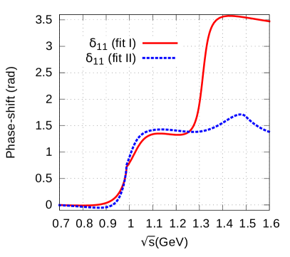
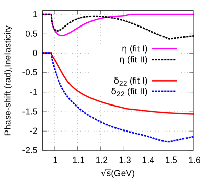
Figure 5: The phase-shifts and the inelasticity from the two-channel $T$-matrix model using the two sets of parameters corresponding to the two $\chi^{2}$ minimums.

At higher energies a clear difference between the two fits is the sharp increase of the $\pi\eta$ phase-shift in fit I around $E\simeq 1.32$ GeV, typical of a narrow resonance, which we will call $a^{\prime}_{0}$. Indeed, one finds a resonance pole in the $T$-matrix located on the third Riemann sheet with the value,

$$\sqrt{s_{a^{\prime}_{0}}}=1315(4)-i\,24(3)\ \hbox{MeV}\qquad(\hbox{fit I})\ .$$ (91)

This resonance is lighter and narrower than the standard $a_{0}(1450)$. Since the phase-shift increases from $\pi/2$ to $\pi$ (approximately) it gives rise to a sharp dip (instead of a peak) in the $S$-wave cross-section. Clearly then, our fit I is quite analogous to the best fit by the Belle collaboration [13] which displays a resonance (called $a_{0}(Y)$ in that reference) which has very similar features while using a parametrisation rather different from ours. The $S$-wave amplitude in fit II also has an $a^{\prime}_{0}$ resonance pole but it is heavier and much broader than that of fit I,

$$\sqrt{s_{a^{\prime}_{0}}}=1421(5)-i\,175(4)\ \hbox{MeV}\qquad(\hbox{fit II})\ .$$ (92)

In this case, the width of the resonance is larger than the experimental one. One eventually does not expect a very accurate determination since the resonance lies close to the cutoff of the model.

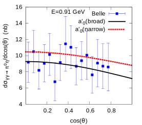
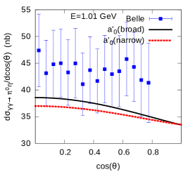
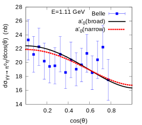
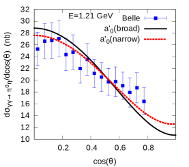
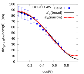
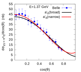
Figure 6: Experimental $\gamma\gamma\to\pi\eta$ differential cross-sections compared with the two fits results.

Fig. 6 and fig. 8 show a sample of $\gamma\gamma\to\pi\eta,K_{S}K_{S}$ differential cross sections comparing the experimental results with those from the two fits. The difference between the two fits is remarkably small, which is somewhat puzzling: why is the narrow $a^{\prime}_{0}$ resonance present in fit I not seen much more clearly? The reason for this arises from a specific interference effect between the $J^{\lambda\lambda^{\prime}}=0^{++}$ and the $2^{++}$ amplitudes. We have seen already that the fast energy variation induced by the narrow $a^{\prime}_{0}$ coincides with that induced by the $a_{2}(1320)$. More specifically, when $\sqrt{s}\simeq 1.32$ GeV, the following relations hold approximately between the $l_{0++}$ and the $l_{2++}$ amplitudes in the case of fit I

$$\begin{array}[]{l}{\rm Re\,}[l_{0++}(s)]\simeq-5{\rm Re\,}[l_{2++}(s)]\\[5.69046pt] {\rm Im\,}[l_{0++}(s)]\simeq-5{\rm Im\,}[l_{2++}(s)]+0.7\ .\end{array}$$ (93)

The sum of the $0^{++}$ and the $2^{++}$ partial-wave amplitudes can effectively be absorbed into the $2^{+-}$ resonance amplitude (since the angular functions satisfy the relation $d^{2}_{00}(\theta)-1=-\sqrt{6}\,d^{2}_{20}(\theta)$) and no specific $0^{++}$ resonance effect remains. We also note that the $a^{\prime}_{0}$ in fit I essentially decouples from the $K\bar{K}$ channel such that no $0^{++}$ resonance effect is seen in this channel either. Because of these fine-tuned relations between the scalar and the tensor resonances the fit I solution is most likely to be unphysical.

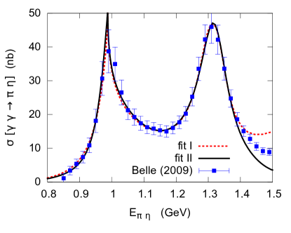
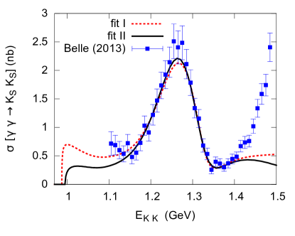
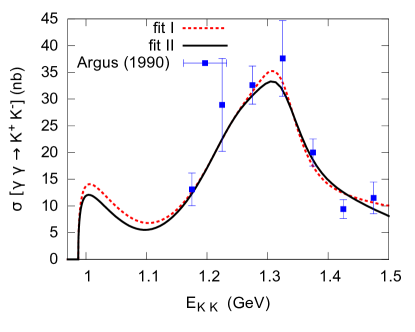
Figure 7: Cross-sections for $\gamma\gamma\to\pi\eta,K_{S}K_{S},{K^{+}}{K^{-}}$ integrated in the range $|\cos\theta|<0.8$. The data are from refs. [13, 16, 43], they are compared with the two fits results.

One can see from fig. 6 that the $\pi\eta$ differential cross-sections are well described except, however, in one energy bin: $E=1.01$ MeV. At this energy, the cross-sections are underestimated by our model, see also fig. 7 which shows the cross-sections integrated over $\theta$. This discrepancy could be caused by an isospin breaking effect close to the resonance peak. Our model assumes isospin symmetry and uses $m_{K}\equiv m_{K^{+}}$ (in order to correctly implement the kaon Born amplitudes) and the peak of the cross-section occurs exactly at $E=2m_{K^{+}}$. Physically, however, the $K^{+}$ and the $K^{0}$ have slightly different masses which should lead to two cusps in the shape of the integrated cross-section. On the experimental side, the energy resolution should be smaller than $2m_{K^{+}}-2m_{K^{0}}\simeq 8$ MeV in order to clearly observe this effect.

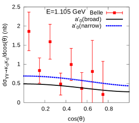
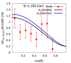
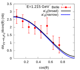
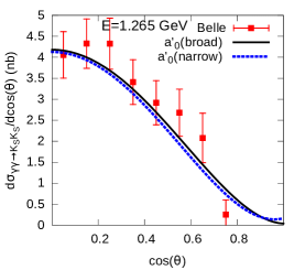
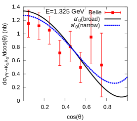
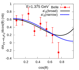
Figure 8: Experimental $\gamma\gamma\to K_{S}K_{S}$ differential cross-sections compared with the two fits results.

The values of the remaining seven parameters included in the fit (subtraction parameter $b_{k}$, tensor mesons to $2\gamma$ coupling constants, $a_{2}$ mass and width) are collected in table 3 below. The couplings $D^{T}_{2\gamma}$ are found, as expected, to be smaller in magnitude than the $C^{T}_{2\gamma}$ although this suppression is only by a factor of two in the case of fit I. The values are in qualitative agreement with the PDG expectations except, however, for the $a_{2}$ mass which is shifted by approximately 10 MeV. This shift is easily seen to be caused by the presence of non-resonant contributions to the $J=2$ amplitudes modelled here by the vector-meson exchanges, $l^{V}_{2,\lambda\lambda^{\prime}}$. The presence of this term is essential for obtaining a correct description of the amplitude in the $\eta$ decay region $s<(m_{\eta}-m_{\pi})^{2}$. In the 1 GeV energy region, one expects some modifications induced by higher mass exchanges, but we see no reason that it should be completely cancelled. We will consider a variation of this term as a source of error below.

	$C^{a_{2}}_{\gamma\gamma}$	$D^{a_{2}}_{\gamma\gamma}$	$C^{f_{2}}_{\gamma\gamma}$	$D^{f_{2}}_{\gamma\gamma}$	$m_{a_{2}}$	$\Gamma_{a_{2}}$	$b_{k}$
fit I	$0.105(2)$	$\phantom{-}0.051(9)$	$0.161(2)$	$0.081(12)$	$1.328(1)$	$0.097(2)$	$-0.254(1)$
fit II	$0.106(2)$	$-0.033(6)$	$0.171(2)$	$0.007(9)$	$1.332(1)$	$0.112(3)$	$-0.167(5)$

Table 3: Values of the coupling constants, of the subtraction constant $b_{k}$ and of the mass and width of the $a_{2}(1320)$ resonance resulting from the two fits.

5.4 Properties of the $a_{0}$ resonances

In this section we consider in more detail the properties of the two $a_{0}$ resonances which can be deduced from our analysis of the photon-photon data. We will focus on the results from fit II since fit I was argued not to be physically relevant. The formulas needed to define the $T$-matrix elements on the unphysical Riemann sheets are given in appendix D. One may define coupling constants from the residues of the resonance poles (e.g. [53] in the context of photon-photon amplitudes), the couplings to the $\pi\eta$ and $K\bar{K}$ channels are thus defined as

$$\left.16\pi T_{11}^{(II)}(z)\right|_{pole}=\frac{g^{2}_{a_{0}\pi\eta}}{z_{a_{0}}-z},\quad\left.16\pi T_{12}^{(II)}(z)\right|_{pole}=\frac{g_{a_{0}\pi\eta}g_{a_{0}K\bar{K}}}{z_{a_{0}}-z}$$ (94)

and similarly for the third Riemann sheet. The coupling to the $\gamma\gamma$ channel and the associated width are defined as

$$\left.e^{2}l_{0++}^{(II)}(z)\right|_{pole}=\frac{g_{a_{0}\gamma\gamma}g_{a_{0}\pi\eta}}{z_{a_{0}}-z},\quad\Gamma_{a_{0}\to\gamma\gamma}=\frac{|g_{a_{0}\gamma\gamma}|^{2}}{16\pi m_{a_{0}}}\ .$$ (95)

The following numerical results are found on sheet II for the position of the $a_{0}(980)$ pole and the corresponding coupling constants

$$\begin{array}[]{ll}\sqrt{s_{a_{0}}}=&1000.7(7)-i\,36.6(1.3)\ (\hbox{MeV})\\[5.69046pt] |g_{a_{0}\pi\eta}|=&2.17(2)\ (\hbox{GeV})\\[5.69046pt] |g_{a_{0}K\bar{K}}|=&4.03(2)\ (\hbox{GeV})\\[5.69046pt] \Gamma_{a_{0}\gamma\gamma}=&0.52(1)\ (\hbox{keV})\ .\end{array}$$ (96)

From the sheet III resonance, the position of the pole was given in eq. (92) and the corresponding coupling constants have the following values

$$\begin{array}[]{ll}|g_{a^{\prime}_{0}\pi\eta}|=&3.15(4)\ (\hbox{GeV})\\[5.69046pt] |g_{a^{\prime}_{0}K\bar{K}}|=&1.89(4)\ (\hbox{GeV})\\[5.69046pt] \Gamma_{a^{\prime}_{0}\gamma\gamma}=&1.05(5)\ (\hbox{keV})\ .\end{array}$$ (97)

	$s_{A}$	$L_{i}$	$c^{\prime}_{m}/c^{\prime}_{d}$	LC(a)	LC(b)	Total
$m_{a_{0}}$ (MeV)	$[-0.2,1.9]$	$5.7$	$[4.2,10.8]$	$1.7$	$[1.9,3.0]$	$[-0.2,12.9]$
$\Gamma_{a_{0}}/2$ (MeV)	$[-2.3,3.7]$	$3.8$	$[7.1,11.0]$	$0.5$	$[0.3,3.0]$	$[-2.3,12.6]$
$|g_{a_{0}\pi\eta}|$ (GeV)	$[-0.15,0.21]$	$0.20$	$[0.21,0.47]$	$0.13$	$[-0.03,0.19]$	$[-0.2,0.6]$
$|g_{a_{0}K\bar{K}}|$ (GeV)	$[-0.03,0.05]$	$-0.13$	$[0.01,0.28]$	$0.05$	$[-0.03,0.04]$	$[-0.2,0.3]$
$\Gamma_{a_{0}\gamma\gamma}$ (keV)	$[-0.05,0.07]$	$0.07$	$[0.06,0.16]$	$0.14$	$[-0.01,0.06]$	$[-0.1,0.2]$
$m_{a^{\prime}_{0}}$ (MeV)	$[2.4,30.2]$	$104.2$	$[22.2,62.3]$	$-11.4$	$[-12.9,53.3]$	$[-17,136]$
$\Gamma_{a^{\prime}_{0}}/2$ (MeV)	$[18.3,44.0]$	$68.2$	$[6.6,14.8]$	$4.2$	$[18.2,66.5]$	$[0,106]$
$|g_{a^{\prime}_{0}\pi\eta}|$ (GeV)	$[-0.68,0.01]$	$-0.28$	$[-0.05,0.10]$	$0.13$	$[-0.89,0.10]$	$[-1.2,0.2]$
$|g_{a^{\prime}_{0}K\bar{K}}|$ (GeV)	$[-0.26,0.06]$	$-0.20$	$[-1.56,-1.42]$	$-0.05$	$[-0.17,-0.07]$	$[-1.6,0.06]$
$\Gamma_{a^{\prime}_{0}\gamma\gamma}$ (keV)	$[0.14,0.22]$	$0.40$	$[-0.28,-0.25]$	$-0.13$	$[0.21,0.17]$	$[-0.3,0.5]$

Table 4: Errors generated by varying the fixed parameters of the $S$-wave amplitudes, columns 5 and 6 refer to the left-cut (see text).

The errors quoted in the above formulas are those arising from the fitted parameters (for which MINUIT provides a correlation matrix). In addition to those, one must consider errors associated with further parameters on which the $T$-matrix depends, which we have assumed to be fixed up to now:

• Adler zero: the value of Adler zero was fixed to $s_{A}=m_{\eta}^{2}$ but its exact value is not known, we will vary it in the range $s_{A}=m_{\eta}^{2}\pm 3m_{\pi}^{2}$.

• Set of the $O(p^{4})$ parameters $L_{i}$: in the BE14 determination [48], their values are given with errors but there are strong correlations. In order to estimate an error from this source we used two different sets of $L_{i}^{\prime}s$ which correspond to two best fits made with different assumptions (second and third column in Table 3 of ref. [48]).

• The ratio of the scalar couplings $c^{\prime}_{m}/c^{\prime}_{d}$ (see eqs. (86), (87)) was varied between 1 and 3 to estimate an uncertainty from this source.

• Left-hand cut: a) we added a contribution from a set of axial-vector mesons and b) we varied the products of the couplings of the vector mesons by $\pm 20\%$.

Table 4 gives the detailed list of the errors generated from these variations on the properties of the two $a_{0}$ resonances.

5.5 The $\eta\to{\pi^{0}}\gamma\gamma$ decay amplitude

We consider now the modelled amplitudes in the kinematical region relevant for the decay $\eta\to{\pi^{0}}\gamma\gamma$. Including the $J=0$ and $J=2$ partial-waves, the distribution as a function of the $\gamma\gamma$ invariant mass squared, $s$, reads

$$\begin{array}[]{ll}\dfrac{d\Gamma^{\eta\to\gamma\gamma\pi}}{ds}=\dfrac{\alpha^{2}}{16\pi m_{\eta}^{3}}\sqrt{\lambda_{12}(s)}&\Big{\{}|l_{0,++}(s)+\tilde{l}_{0,++}(s)|^{2}+5\,|l^{V}_{2,++}(s)+l^{BW}_{2,++}(s)|^{2}\\[8.5359pt] &+5\,|l^{V}_{2,+-}(s)+l^{BW}_{2,+-}(s)|^{2}\Big{\}}\end{array}$$ (98)

also accounting for the $J=0$ isospin violating amplitude $\tilde{l}_{0,++}$.

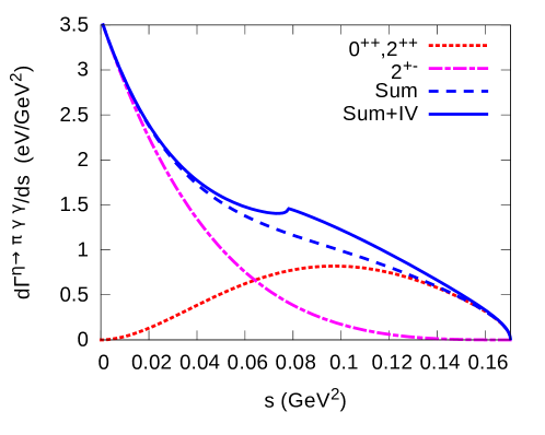
Figure 9: Contributions to the $\eta\to\pi^{0}\gamma\gamma$ energy distribution from the amplitudes fitted in the scattering region. Dotted line (red): $S$-wave (isospin conserving) and $2^{++}$ $D$-wave, dash-dotted line (magenta): $2^{+-}$ $D$-wave, dashed line: sum of the $S$ and $D$ waves, solid line: sum including the isospin violating amplitude $\tilde{l}_{0++}$.

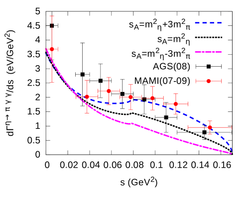
Figure 10: Experimental data on the $\eta\to\pi^{0}\gamma\gamma$ energy distribution [14, 15] compared with predictions from our amplitudes showing the influence of the position of the Adler zero.

Fig.9 illustrates the contributions of the various amplitudes corresponding to central values of the parameters fitted in the scattering region. The $2^{+-}$ partial-wave dominates over the other ones near $s=0$ because the $J^{++}$ amplitudes are suppressed by the soft-photon zero. The relative role of the $S$-wave increases with the energy and starts to be dominating above the $\pi^{+}\pi^{-}$ threshold. The figure also shows that the isospin-violating $S$-wave generates a visible cusp at this threshold. The central value of the decay width generated by our amplitudes is $\Gamma=0.237$ eV which is on the low side of the most recent experimental determinations $\Gamma_{exp}=0.285\pm 0.031\pm 0.061$ eV (Crystal Ball at the AGS [14]), $\Gamma_{exp}=0.33\pm 0.03$ eV (MAMI [15]). A smaller value was reported by the KLOE-2 collaboration [55] but it has not been confirmed and the data is currently being reanalysed. The amplitudes in the $\eta$ decay region are very sensitive to the precise position of the Adler zero. This is illustrated in fig. 10 showing the effect of varying $s_{A}$ in the range $[m_{\eta}^{2}-3m_{\pi}^{2},m_{\eta}^{2}+3m_{\pi}^{2}]$ and comparing with the experimental results. Given somewhat more precise data the value of $s_{A}$ could be included in the fitting. The amplitudes in the decay region are also sensitive to the vector meson coupling constants, the value of which dominate the energy distribution near $s=0$. Accounting for these main errors we would predict

$$\Gamma^{\eta\to{\pi^{0}}\gamma\gamma}=0.237^{+0.060}_{-0.043}\ \hbox{eV}\ .$$ (99)

6 Conclusions

In this work we have reconsidered the properties of the light isovector scalar resonances as can be determined from photon-photon scattering experimental results. For this purpose, we have implemented a standard Muskhelishvili-Omnès integral representation for the $J=0$ amplitude in which the left-cut is modelled from light vector meson exchanges. The underlying $T$-matrix satisfies unitarity with two channels ($\pi\eta,K\bar{K}$) and involves six phenomenological parameters. In the case of the $J=2$ amplitudes the constraints from unitarity are more difficult to implement, a cruder description is used which consists in simply adding the cross-channel vector-exchange and the direct channel tensor resonance amplitudes. In order to constrain the free parameters as unambiguously as possible we performed fits to both $\pi\eta$ and $K_{S}K_{S}$ data, for which high-statistics data below 1.4 GeV are available at present, and we found two different acceptable solutions to the minimisation. Both solutions are also compatible with the available $K^{+}K^{-}$ data from the ARGUS collaboration [43].

In one of our fits the $S$-wave amplitude displays a light and narrow $a^{\prime}_{0}$ resonance exactly similar to the one found in the Belle analysis. While this is mathematically allowed we have argued that the fit which displays a broad $a^{\prime}_{0}$ is likely to be more physical. Concerning the $a_{0}(980)$ resonance, we find that a rather conventional picture i.e. a pole on the second sheet with a mass and width compatible with the PDG and coupling to both the $\pi\eta$ and the $K\bar{K}$ channels is perfectly compatible with both the $\pi\eta$ and the $K_{S}K_{S}$ data. This is in contrast with the Belle analysis which uses an elastic Breit-Wigner description and also with the recent analysis of ref. [18] in which the mass and width are found to be both significantly larger than the PDG values. Data with a better energy resolution would be useful to resolve these remaining ambiguities. The $\gamma\gamma\to{K^{+}}{K^{-}},K_{S}K_{S}$ cross-sections close to the $K\bar{K}$ thresholds are also very sensitive to the position of the $a_{0}(980)$. Our results in this energy region are in qualitative agreement with the chiral-unitary calculations from ref. [29] and with the estimates made in ref. [56] but not with those from ref. [26]. Experimental data in this near-thresold region would obviously be very constraining. Finally, it will be quite interesting to see how the pole position determined in a lattice QCD simulation [22] evolves when the value of $m_{\pi}$ is decreased.

Acknowledgements
We would like to thank prof. S. Uehara for many clarifying explanations about the Belle experiments. JXL thanks Prof. Lisheng Geng for useful discussions. JXL is partly supported by the National Natural Science Foundation of China under Grant Nos.11735003, 11975041, 11961141004 and by the Fundamental Research Funds for the Central Universities. He also gratefully acknowledges the financial support from the China Scholarship Council. This work is supported in part by the European Union’s Horizon2020 research and innovation programme (HADRON-2020) under the Grant Agreement n^∘ 824093.

Appendix A Scalar form factors

In this section we consider how the two isovector scalar form factors get modified as compared to the results of ref. [27] when using the set of $T$-matrix parameters as determined here from the $\gamma\gamma$ data. The form factors were defined as

$$\begin{array}[]{l}B_{0}F_{S}^{\eta\pi}(s)={\langle\eta{\pi^{+}}|\,\bar{u}d(0)\,|0\rangle}\\[5.69046pt] B_{0}F_{S}^{K\bar{K}}(s)={\langle{\bar{K}^{0}}{K^{+}}|\,\bar{u}d(0)\,|0\rangle}\end{array}$$ (100)

where $B_{0}$ is the chiral coupling proportional to the quark condensate [47]

$$B_{0}=-\left.{\langle 0|\bar{u}{u}|0\rangle}/F^{2}_{\pi}\right|_{m_{u}=m_{d}=m_{s}=0}\ .$$ (101)

Under the assumption of two-channel unitarity these form factors, we recall, are simply related to the MO matrix,

$$\begin{pmatrix}F_{S}^{\eta\pi}(s)\\[5.69046pt] F_{S}^{K\bar{K}}(s)\end{pmatrix}=\bm{\Omega}_{0}(s)\times\begin{pmatrix}F_{S}^{\eta\pi}(0)\\[5.69046pt] F_{S}^{K\bar{K}}(0)\end{pmatrix}\ .$$ (102)

The values at $s=0$ are estimated from the chiral expansion at order $p^{4}$. In ref. [27] the set of $L_{i}$ values from ref. [48] based on a $p^{4}$ fit was used while here we preferred to use a set from a $p^{6}$ fit (BE14 set), which gives

$$\begin{array}[]{l}F_{S}^{\eta\pi}(0)=0.972\\[2.84544pt] F_{S}^{K\bar{K}}(0)=0.845\ .\end{array}$$ (103)

Interesting quantities which are related to the scalar form factors are the scalar radii which are proportional to their derivatives at $s=0$

$${\langle r^{2}\rangle}_{S}^{P_{1}P_{2}}\equiv 6\dot{F}_{S}^{P_{1}P_{2}}(0)/{F}_{S}^{P_{1}P_{2}}(0)\ .$$ (104)

At chiral order $p^{4}$ the scalar radii depend on a single low-energy coupling, $L_{5}$. Using its value from the BE14 set, $L^{r}_{5}=(1.01\pm 0.06)\cdot 10^{-3}$, gives

$$\begin{array}[]{l}\left.{\langle r^{2}\rangle}_{S}^{\eta{\pi^{+}}}\right|_{p^{4}}=0.067(7)\ \hbox{fm}^{3}\\[2.84544pt] \left.{\langle r^{2}\rangle}_{S}^{K\bar{K}}\right|_{p^{4}}=0.111(7)\ \hbox{fm}^{3}\ .\end{array}$$ (105)

Fig. 11 shows the absolute values of the form factors using the BE14 chiral couplings and the set of $T$-matrix parameters fitted to the $\gamma\gamma$ data. The $a_{0}(980)$ resonance displays a smaller peak than in ref. [27] and its position is slightly shifted, reflecting the modified position of the pole. The $a^{\prime}_{0}$ resonance also differs: in the case of the “narrow $a^{\prime}_{0}$” fit solution it shows up as a dip in the $\eta\pi$ form factor while in the case of the “broad $a^{\prime}_{0}$” solution its effect is hardly visible. Concerning the scalar radii, the dispersive amplitudes give

$$\begin{array}[]{l}{\langle r^{2}\rangle}_{S}^{\eta\pi}=\left(2.73^{+4.10}_{-2.60}\right)\cdot 10^{-2}\ \hbox{fm}^{2}\\[5.69046pt] {\langle r^{2}\rangle}_{S}^{K\bar{K}}=0.156^{+0.002}_{-0.029}\ \hbox{fm}^{2}\ .\end{array}$$ (106)

These results correspond to fit solutions with a “broad” $a^{\prime}_{0}$. As compared with the the chiral $O(p^{4})$ result, the central value is somewhat too small in the case of $\eta\pi$ and too large in the case of $K\bar{K}$.

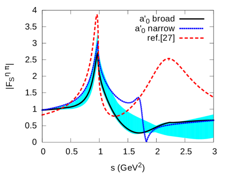
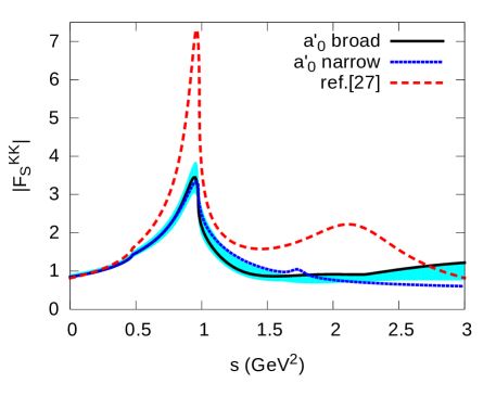
Figure 11: Absolute values of the scalar form factors: the results using the sets of $T$-matrix parameters from the two different fits to the $\gamma\gamma$ data are compared with a typical result from ref. [27]. The bands are obtained by varying the intrinsic parameters as in table 4.

Appendix B Chiral expansion results for $\gamma\gamma\to P_{1}P_{2}$ amplitudes

B.1 Order $p^{4}$

We collect below the expressions of the photon-photon amplitudes in the chiral expansion at order $p^{4}$. The chiral order $p^{2}$ coincides with scalar QED and gives rise to the Born amplitudes for ${\pi^{+}}{\pi^{-}}$ and ${K^{+}}{K^{-}}$ which were given in eq. (35). The leading contributions to the amplitudes which involve two neutral mesons: $\pi^{0}\pi^{0}$, ${K^{0}}{\bar{K}^{0}}$ and ${\pi^{0}}\eta$ appear at order $p^{4}$. They were computed in refs. [57, 58, 59, 33]. The basic one-loop function which occurs in these $p^{4}$ amplitudes can be written as,

$$G_{P}(z)=-1-\frac{m_{P}^{2}}{z}\left(\log\dfrac{\sqrt{1-4m_{P}^{2}/z}+1}{\sqrt{1-4m_{P}^{2}/z}-1}\right)^{2}\ ,$$ (107)

for small $z$ values, $|z|<<m_{P}^{2}$, it behaves as

$$G_{P}(z)=\dfrac{z}{12m_{P}^{2}}+O(z^{2})\ .$$ (108)

The expression for the $\gamma\gamma\to\pi^{0}\pi^{0}$ scalar amplitudes at $O(p^{4})$ read,

$$\begin{array}[]{l}A_{NLO}^{{\pi^{0}}{\pi^{0}}}(s,t,u)=\dfrac{1}{4\pi^{2}\,s}\bigg{[}\dfrac{s-m_{\pi}^{2}}{F_{\pi}^{2}}G_{\pi}(s)+\dfrac{s}{4F_{\pi}^{2}}G_{K}(s)\bigg{]}\\[5.69046pt] B_{NLO}^{{\pi^{0}}{\pi^{0}}}(s,t,u)=0\ .\end{array}$$ (109)

These formulas illustrate general features: the $O(p^{4})$ part of the $A$ amplitudes have a simple structure involving a sum of products of meson-meson amplitudes at order $p^{2}$ with one-loop functions $G_{P}$ while the $B$ amplitudes vanish at this order. Next, the expression for $\gamma\gamma\to{K^{0}}{\bar{K}^{0}}$ at $O(p^{4})$ reads

$$\begin{array}[]{l}A_{NLO}^{{K^{0}}{\bar{K}^{0}}}(s,t,u)=\dfrac{1}{4\pi^{2}\,s}\bigg{[}\dfrac{s}{4F_{\pi}^{2}}\,G_{\pi}(s)+\dfrac{s}{4F_{\pi}^{2}}\,G_{K}(s)\bigg{]}\ .\\ \end{array}$$ (110)

The NLO expression for the $\gamma\gamma\to{\pi^{0}}\eta$ amplitude, which is of particular interest here, was worked out in ref. [33]. They considered a chiral framework which also includes the $\eta^{\prime}$ meson as a light meson in addition to the pseudo-Goldstone octet. The relation between the $\eta$ and $\eta^{\prime}$ mesons and the octet and singlet chiral fields involves a mixing angle $\theta$,

$$\begin{array}[]{l}\eta=c_{\theta}\,\phi^{8}-s_{\theta}\,\phi^{0}\\ \eta^{\prime}=s_{\theta}\,\phi^{8}+c_{\theta}\,\phi^{0}\end{array}$$ (111)

denoting $c_{\theta}=\cos\theta$, $s_{\theta}=\sin\theta$. The expression for the $\gamma\gamma\to{\pi^{0}}\eta$ amplitude as a function of $\theta$ reads,

$$\begin{array}[]{l}A_{NLO}^{{\pi^{0}}\eta}(s,t,u)=\dfrac{1}{4\pi^{2}\,s}\bigg{[}\dfrac{\sqrt{3}\,c_{\theta}}{36F_{\pi}^{2}}\big{(}9s-m_{\pi}^{2}-8m_{K}^{2}-3m_{\eta}^{2}-\sqrt{8}t_{\theta}(m_{\pi}^{2}+2m_{K}^{2})\big{)}\,G_{K}(s)\\[8.5359pt] \quad+\dfrac{B_{0}(m_{d}-m_{u})}{3\sqrt{3}(m_{\eta}^{2}-m_{\pi}^{2})F_{\pi}^{2}}\big{(}(c_{\theta}-\sqrt{2}s_{\theta})(4m_{\pi}^{2}-3s)-t_{\theta}(4\sqrt{2}c_{\theta}+s_{\theta})m_{\pi}^{2}\big{)}\,G_{\pi}(s)\bigg{]}\\[14.22636pt] \end{array}$$ (112)

with $t_{\theta}=\tan\theta$. The isospin conserving part in eq. (112) agrees with ref. [60]. It reproduces the result from ref. [33] upon setting $s_{\theta}=-1/3$, $c_{\theta}=\sqrt{8}/3$ and neglecting the terms proportional to $t_{\theta}$ (which are not really negligible). In the standard ChPT one must set $c_{\theta}=1$, $s_{\theta}=0$ at leading order. Doing so, the amplitude simplifies significantly and reads

$$\begin{array}[]{l}A_{NLO}^{{\pi^{0}}\eta}(s,t,u)=\dfrac{1}{4\pi^{2}\,s}\bigg{[}\dfrac{3s-4m_{K}^{2}}{4\sqrt{3}F_{\pi}^{2}}\,G_{K}(s)\\[11.38092pt] \quad+\dfrac{B_{0}(m_{d}-m_{u})}{m_{\eta}^{2}-m_{\pi}^{2}}\,\dfrac{4m_{\pi}^{2}-3s}{3\sqrt{3}F_{\pi}^{2}}\big{(}G_{\pi}(s)-\frac{1}{2}G_{K}(s)\big{)}\bigg{]}\end{array}$$ (113)

where the Gell-Mann-Okubo mass relation was used and the kaon loop contribution to the isospin violating part was included for completeness. The quantity $B_{0}(m_{d}-m_{u})$ is given at leading chiral order by

$$B_{0}(m_{d}-m_{u})=\left(m^{2}_{K^{0}}-m^{2}_{K^{+}}\right)_{QCD}\ .$$ (114)

Let us quote also the formula for $\gamma\gamma\to\eta\eta$

$$\begin{array}[]{l}A^{\eta\eta}_{NLO}(s,t,u)=\dfrac{1}{4\pi^{2}s}\bigg{[}\dfrac{m_{\pi}^{2}}{3F_{\pi}^{2}}\,G_{\pi}(s)+\dfrac{9s-8m_{K}^{2}}{12F_{\pi}^{2}}\,G_{K}(s)\bigg{]}\ .\\ \end{array}$$ (115)

Finally, the order $p^{4}$ contributions to the $\gamma\gamma\to{\pi^{+}}{\pi^{-}}$ and ${K^{+}}{K^{-}}$ amplitudes read

$$\begin{array}[]{l}A^{{\pi^{+}}{\pi^{-}}}_{NLO}(s,t,u)=\dfrac{8}{F_{\pi}^{2}}(L_{9}^{r}+L_{10}^{r})+\dfrac{1}{4\pi^{2}\,s}\bigg{[}\dfrac{s}{2F_{\pi}^{2}}\,G_{\pi}(s)+\dfrac{s}{4F_{\pi}^{2}}\,G_{K}(s)\bigg{]}\\ \end{array}$$ (116)

and

$$\begin{array}[]{l}A^{{K^{+}}{K^{-}}}_{NLO}(s,t,u)=\dfrac{8}{F_{\pi}^{2}}(L_{9}^{r}+L_{10}^{r})+\dfrac{1}{4\pi^{2}\,s}\bigg{[}\dfrac{s}{4F_{\pi}^{2}}\,G_{\pi}(s)+\dfrac{s}{2F_{\pi}^{2}}\,G_{K}(s)\bigg{]}\ .\\ \end{array}$$ (117)

Combining eqs. (110) and (117) we get the NLO part of the $\gamma\gamma\to(K\bar{K})^{I=1},\,(K\bar{K})^{I=0}$ amplitudes

$$\begin{array}[]{l}A_{NLO}^{(K\bar{K})^{1}}=-\dfrac{4\sqrt{2}}{F_{\pi}^{2}}(L_{9}+L_{10})-\dfrac{\sqrt{2}\,}{4\pi^{2}\,s}\bigg{[}\dfrac{s}{8F_{\pi}^{2}}G_{K}(s)\bigg{]}\\[8.5359pt] A_{NLO}^{(K\bar{K})^{0}}=-\dfrac{4\sqrt{2}}{F_{\pi}^{2}}(L_{9}+L_{10})-\dfrac{\sqrt{2}\,}{4\pi^{2}\,s}\bigg{[}\dfrac{s}{4F_{\pi}^{2}}G_{\pi}(s)+\dfrac{3s}{8F_{\pi}^{2}}G_{K}(s)\bigg{]}\ .\end{array}$$ (118)

B.2 Soft pion limit (isospin conserving part)

Let us consider a limit when the pion in the $\gamma\gamma\to{\pi^{0}}\eta$ amplitude becomes “soft” i.e. $p_{1}=0$. This limit is unphysical but it allows to obtain exact results which should hold for the physical amplitude modulo $O(m_{\pi}^{2})$ corrections. In this limit, firstly, one has

$$s=m_{\eta}^{2},\quad t=u=0\quad(\hbox{soft pion limit})\ ,$$ (119)

and using standard soft pion methods one shows that the amplitude $\gamma\gamma\to{\pi^{0}}\eta$ vanishes exactly at this point. When $p_{1}=0$ the two tensors $T^{\mu\nu}_{1}$, $T^{\mu\nu}_{2}$ become degenerate

$$T^{\mu\nu}_{2}=2m_{\eta}^{2}\,T^{\mu\nu}_{1}$$ (120)

such that the soft limit amplitude, in tensorial form, reads

$$\lim_{p_{1}\to 0}W^{\mu\nu}(q_{1},q_{2};p_{1},p_{2})=(A(m_{\eta}^{2},0)+2m_{\eta}^{2}B(m_{\eta}^{2},0))\,T_{1}^{\mu\nu}=0\ .$$ (121)

The combination which appears in eq. (121) is the helicity amplitude $L_{++}$ in the soft pion limit. This implies that the physical helicity amplitude $L_{++}$ with $t=u$ should also have an Adler zero as a function of $s$,

$$L_{++}(s_{A},t=u)=0$$ (122)

with $s_{A}=m_{\eta}^{2}+O(m_{\pi}^{2})$. Let us consider the implication of this result for the $j=0$ partial wave. The expansion of the helicity amplitude with $\cos\theta=0$ (which corresponds to $t-u=0$) reads

$$L_{++}(s,\cos\theta=0)=\sum_{j\ even}(2j+1)\,(-1)^{j/2}\frac{(j-1)!!}{j!!}\,l_{j,++}(s)\ .$$ (123)

When $s=m_{\eta}^{2}$, the amplitudes with $j\geq 2$ are suppressed by the angular momentum barrier factor: $l_{2,++}(m_{\eta}^{2})=O(m_{\pi}^{2})$, $l_{4,++}(m_{\eta}^{2})=O(m_{\pi}^{4}),\cdots$. The soft pion condition therefore implies that the $j=0$ partial-wave should satisfy $l_{0,++}(m_{\eta}^{2})=O(m_{\pi}^{2})$ such that an Adler zero should be present in this partial-wave amplitude,

$$l_{0,++}(s_{A})=0\ .$$ (124)

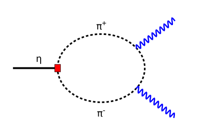
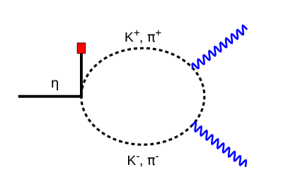
Figure 12: Representative chiral one-loop diagrams contributing to the matrix element of the operator $p_{0}=i(\bar{u}\gamma^{5}{u}+\bar{d}\gamma^{5}{d})$ needed in the soft-pion relation (128). Insertions of $p_{0}$ are represented by a red square.

B.3 Soft pion limit (isospin violating part)

In the case of the isospin violating piece of the $\gamma\gamma\to{\pi^{0}}\eta$ amplitude, the soft pion limit does not lead to an Adler zero. Let us define this amplitude in terms of the following matrix element,

$$\tilde{L}_{++}\equiv{\langle{\pi^{0}}(p_{1})\eta(p_{2})|\frac{1}{2}(m_{d}-m_{u})(\bar{u}u-\bar{d}{d})|\gamma(q_{1},+)\gamma(q_{2},+)\rangle}\ ,$$ (125)

which involves the isospin violating part of the QCD Lagrangian. Using the usual soft pion techniques, the soft pion limit of this amplitude is expressed in terms of the commutator

$$\lim_{p_{1}\to 0}\tilde{L}_{++}=-\dfrac{i}{2F_{\pi}}{\langle\eta(p_{2})|(m_{d}-m_{u})[Q_{5}^{3},(\bar{u}u-\bar{d}{d})]|\gamma(q_{1},+)\gamma(q_{2},+)\rangle}\ .$$ (126)

where $Q_{5}^{3}$ is the axial charge

$$Q_{5}^{3}=\frac{1}{2}\int d^{3}x(\bar{u}\gamma^{0}\gamma^{5}{u}-\bar{d}\gamma^{0}\gamma^{5}{d})(0,x)\ .$$ (127)

The commutator is easily worked out and gives

$$\lim_{p_{1}\to 0}\tilde{L}_{++}=\dfrac{(m_{d}-m_{u})}{2F_{\pi}}{\langle\eta(p_{2})|i(\bar{u}\gamma^{5}{u}+\bar{d}\gamma^{5}{d})|\gamma(q_{1},+)\gamma(q_{2},+)\rangle}\ .$$ (128)

The matrix element which appears on the right-hand side is a non-perturbative quantity. We can estimate it using the chiral expansion at NLO. The pseudoscalar operator $p_{0}=i(\bar{u}\gamma^{5}{u}+\bar{d}\gamma^{5}{d})$ can couple either to a single $\eta$ meson or to $\eta\pi^{+}\pi^{-}$. Representative one-loop diagrams are shown in fig. 12. Computing them gives

$${\langle\eta(p_{2})|p_{0}(0)|\gamma(q_{1},+)\gamma(q_{2},+)\rangle}_{NLO}=\dfrac{-B_{0}}{4\pi^{2}\,\sqrt{3}F_{\pi}}\,\big{(}1-\dfrac{m_{\pi}^{2}}{3F_{\pi}^{2}}\big{)}\,\big{(}G_{\pi}(m_{\eta}^{2})-\frac{1}{2}G_{K}(m_{\eta}^{2})\big{)}\ .$$ (129)

As one might expect, using this result in the soft pion relation (128) reproduces the isospin violating amplitude at chiral order $p^{4}$ when $s=m_{\eta}^{2}$ (see eq. (113)), up to $O(m_{\pi}^{4}/m^{4}_{\eta})$ terms. In practice, one can relate $(m_{d}-m_{u})B_{0}$ to the QCD kaon mass difference $(m^{2}_{K^{0}}-m^{2}_{K^{0}})_{QCD}$ and then use eq. (28) in order to express $\tilde{l}_{0++}(m_{\eta}^{2})$ in terms of $\epsilon_{L}$. The chiral calculation (129) of the matrix element should be reliable at the $20-30\%$ level since there are no potentially large $p^{6}$ contributions from light vector meson exchanges in this case.

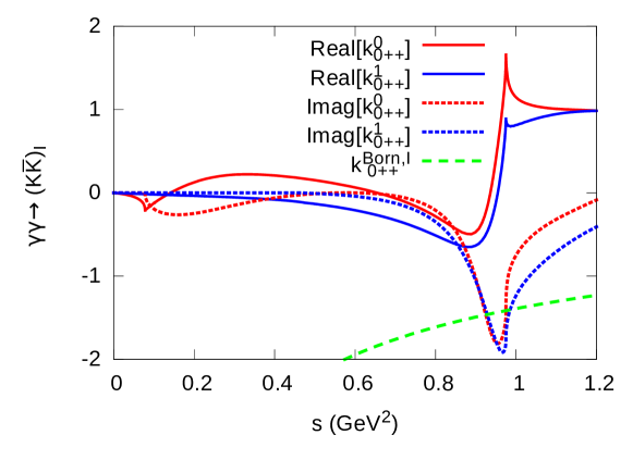
Figure 13: Dispersive $\gamma\gamma\to(K\bar{K})_{I}$ $S$-waves with $I=0,1$ without the Born amplitude which is shown separately.

Appendix C Dispersive $\gamma\gamma\to\pi\pi,\ (K\bar{K})_{I=0}$ $S$-waves

Input for the $\gamma\gamma\to(K\bar{K})_{I=0}$ $S$-wave is needed in order to reconstruct the amplitudes for the physical $K^{+}K^{-}$ and $K_{S}K_{S}$ states. We briefly recall the dispersive coupled-channel representation for the $I=0$ $S$-wave taken from ref. [28]. It has the following form

$$\begin{pmatrix}h_{0++}(s)\\[8.5359pt] k^{0}_{0++}(s)\end{pmatrix}=\begin{pmatrix}h^{Born}_{0++}(s)\\[8.5359pt] k^{0,Born}_{0++}(s)\end{pmatrix}+\bm{\Omega}^{(0)}(s)\begin{pmatrix}b^{0}\,s+b^{{}^{\prime}0}\,s^{2}+L^{(0)}_{1}(s)+R^{(0)}_{1}(s)\\[8.5359pt] b^{0}_{K}\,s+b^{{}^{\prime}0}_{K}\,s^{2}+L^{(0)}_{2}(s)+R^{(0)}_{2}(s)\end{pmatrix}$$ (130)

which is analogous to eqs. (59) for the $I=1$ amplitudes but more subtraction parameters had to be introduced. In eq. (130) $\bm{\Omega}^{(0)}$ is the $I=0$ Omnès matrix and the functions $L^{(0)}_{i}(s)$ ($R^{(0)}_{i}(s)$) are dispersive integrals on the left (right)-hand cuts which are analogous to the corresponding integrals in eqs. (59). The parameter $b^{0}_{K}$ was simply fixed by matching to the $O(p^{4})$ amplitude at $s=0$ (see eq. (118)). The three parameters $b^{0}$, $b^{{}^{\prime}0}$, $b^{{}^{\prime}0}_{K}$ where then determined from fits to $\gamma\gamma\to{\pi^{+}}{\pi^{-}},{\pi^{0}}{\pi^{0}}$ data. Having done so the $K\bar{K}$ amplitude $k^{0}_{0++}$ was generated, which we have used in the present work together with the $I=1$ amplitude. Fig. 13 shows the dispersive results for these two $K\bar{K}$ amplitudes. At low energies the amplitude $k^{0}_{0++}$ is significantly larger in magnitude than $k^{1}_{0++}$ because it gets isoscalar $\pi\pi$ rescattering contributions (which contain the broad $\sigma$ resonance). In the low-energy region, furthermore, the Born amplitude is much larger than the rescattering contributions, in accordance with the chiral counting. In the 1 GeV region the $I=0,1$ rescattering amplitudes are rather similar which leads to a strong suppression of the ${K^{0}}{\bar{K}^{0}}$ cross-section as compared to the ${K^{+}}{K^{-}}$ one close to the $K\bar{K}$ threshold.

Appendix D The $T$-matrix on the four Riemann sheets

The second sheet extension of a matrix elements $T_{ij}$ is defined such as to continue $T_{ij}(z)$ analytically across the cut, below the first inelastic threshold,

$$T^{(II)}_{ij}(s-i\epsilon)=T_{ij}(s+i\epsilon),\quad(m_{\eta}+m_{\pi})^{2}\leq s\leq 4m_{K}^{2}\ .$$ (131)

Using the elastic unitarity relation it easy to find an explicit expression for $T^{(II)}_{ij}$,

$$\bm{T}^{(II)}(z)=\left(1-2\bm{T}(z)\begin{pmatrix}\tilde{\sigma}_{\pi\eta}(z)&0\\ 0&0\\ \end{pmatrix}\right)^{-1}\bm{T}(z)$$ (132)

with

$$\tilde{\sigma}_{\pi\eta}(z)=\frac{\sqrt{(z-m_{-}^{2})(m_{+}^{2}-z)}}{z}\ .$$ (133)

The second sheet extensions of the $\gamma\gamma$ amplitudes $l_{0++}$ and $k_{0++}$ are expressed in a similar way,

$$\begin{pmatrix}l_{0++}^{(II)}(z)\\[5.69046pt] k_{0++}^{(II)}(z)\end{pmatrix}=\left(1-2\bm{T}(z)\begin{pmatrix}\tilde{\sigma}_{\pi\eta}(z)&0\\[5.69046pt] 0&0\\ \end{pmatrix}\right)^{-1}\begin{pmatrix}l_{0++}(z)\\[5.69046pt] k_{0++}(z)\end{pmatrix}\ .$$ (134)

The third sheet extension of the $T$-matrix elements are defined such as to obey continuity equations across the unitarity cut above $4m_{K}^{2}$

$$T_{ij}^{(III)}(s-i\epsilon)=T_{ij}(s+i\epsilon),\quad 4m_{K}^{2}\leq s<\infty\ .$$ (135)

They are easily expressed in matrix form

$$\bm{T}^{(III)}(z)=\left(1-2\bm{T}(z)\begin{pmatrix}\tilde{\sigma}_{\pi\eta}(z)&0\\ 0&\tilde{\sigma}_{KK}(z)\\ \end{pmatrix}\right)^{-1}\,\bm{T}(z)$$ (136)

where $\tilde{\sigma}_{KK}(z)=\sqrt{4m_{K}^{2}/z-1}$. Finally, the fourth sheet extensions of the $T$-matrix elements are given by

$$\bm{T}^{(IV)}(z)=\left(1-2\bm{T}(z)\begin{pmatrix}0&0\\ 0&\tilde{\sigma}_{KK}(z)\\ \end{pmatrix}\right)^{-1}\,\bm{T}(z)$$ (137)

they satisfy continuity equations with $T^{(II)}_{ij}(z)$ when $s>4m_{K}^{2}$ and with $T^{(III)}_{ij}(z)$ when $(m_{\eta}+m_{\pi})^{2}<s<4m_{K}^{2}$.

In our model, the right-cut structure of $T$-matrix is generated by the pair of loop functions $\bar{J}_{\pi\eta}(s)$, $\bar{J}_{KK}(s)$ which can be written as

$$\bar{J}_{12}(z)\equiv\bar{J}^{I}_{12}(z)=\frac{z}{16\pi^{2}}\int_{(m_{1}+m_{2})^{2}}^{\infty}ds^{\prime}\,\frac{\sqrt{\lambda_{12}(s^{\prime})}}{(s^{\prime})^{2}(s^{\prime}-z)}\ .$$ (138)

This expression defines $\bar{J}_{12}$ on the first Riemann sheet and shows that it is analytic except for a cut on $[(m_{1}+m_{2})^{2},\infty]$. The second sheet extension of $\bar{J}_{12}$ is given by

$$\bar{J}^{II}_{12}(z)=\bar{J}_{12}(z)+2\,\frac{\tilde{\sigma}_{12}(z)}{16\pi}\ .$$ (139)

which satisfies the continuity equation $\bar{J}^{II}_{12}(s-i\epsilon)=\bar{J}_{12}(s+i\epsilon)$ when $s\geq(m_{1}+m_{2})^{2}$. The $T$ matrix on the four Riemann sheets can then also be defined as follows in terms of the pair of loop functions

$$\begin{array}[]{ll}T^{I}(z):&(\bar{J}^{I}_{\pi\eta}(z),\bar{J}^{I}_{KK}(z))\\[5.69046pt] T^{II}(z):&(\bar{J}^{II}_{\pi\eta}(z),\bar{J}^{I}_{KK}(z))\\[5.69046pt] T^{III}(z):&(\bar{J}^{II}_{\pi\eta}(z),\bar{J}^{II}_{KK}(z))\\[5.69046pt] T^{IV}(z):&(\bar{J}^{I}_{\pi\eta}(z),\bar{J}^{II}_{KK}(z))\ .\\ \end{array}$$ (140)

Using the $K$-matrix type representation (83) of the $T$-matrix one easily verifies that these definitions satisfy the relevant equations (132), (136), (137) written above.

References

- [1] E. Klempt, A. Zaitsev, Phys.Rept. 454, 1 (2007), 0708.4016
- [2] A. Astier, L. Montanet, M. Baubillier, J. Duboc, Phys.Lett. B25, 294 (1967)
- [3] R. Ammar, R. Davis, W. Kropac, J. Mott, D. Slate, B. Werner, M. Derrick, T. Fields, F. Schweingruber, Phys. Rev. Lett. 21, 1832 (1968)
- [4] S.M. Flatté, Phys.Lett. B63, 224 (1976)
- [5] M. Tanabashi et al. (Particle Data Group), Phys. Rev. D98(3), 030001 (2018)
- [6] F. Jegerlehner, A. Nyffeler, Phys.Rept. 477, 1 (2009), 0902.3360
- [7] F. Low, Phys.Rev. 110, 974 (1958)
- [8] H.D.I. Abarbanel, M.L. Goldberger, Phys. Rev. 165, 1594 (1968)
- [9] S.L. Adler, Phys. Rev. 139, B1638 (1965)
- [10] D. Morgan, M. Pennington, Phys.Lett. B192, 207 (1987)
- [11] D. Morgan, M.R. Pennington, Phys. Lett. B272, 134 (1991), [Erratum: Nucl. Phys.B376, 444 (1992)]
- [12] D. Antreasyan et al. (Crystal Ball), Phys. Rev. D33, 1847 (1986)
- [13] S. Uehara et al. (Belle), Phys.Rev. D80, 032001 (2009), 0906.1464
- [14] S. Prakhov et al., Phys. Rev. C78, 015206 (2008)
- [15] B.M.K. Nefkens et al. (A2 at MAMI), Phys. Rev. C90(2), 025206 (2014), 1405.4904
- [16] S. Uehara et al. (Belle), PTEP 2013(12), 123C01 (2013), 1307.7457
- [17] K. Abe et al. (Belle), Eur. Phys. J. C32, 323 (2003), hep-ex/0309077
- [18] I. Danilkin, O. Deineka, M. Vanderhaeghen, Phys. Rev. D96(11), 114018 (2017), 1709.08595
- [19] I.V. Danilkin, L.I.R. Gil, M.F.M. Lutz, Phys. Lett. B703, 504 (2011), 1106.2230
- [20] N.L. Muskhelishvili, Singular Integral Equations (P. Noordhof, Groningen, 1953)
- [21] R. Omnès, Nuovo Cim. 8, 316 (1958)
- [22] J.J. Dudek, R.G. Edwards, D.J. Wilson (Hadron Spectrum), Phys. Rev. D93(9), 094506 (2016), 1602.05122
- [23] M. Lüscher, Nucl. Phys. B354, 531 (1991)
- [24] Z.H. Guo, L. Liu, U.G. Meißner, J.A. Oller, A. Rusetsky, Phys. Rev. D95(5), 054004 (2017), 1609.08096
- [25] N. Achasov, G. Shestakov, Phys.Rev. D81, 094029 (2010), 1003.5054
- [26] L.Y. Dai, M.R. Pennington, Phys. Rev. D90(3), 036004 (2014), 1404.7524
- [27] M. Albaladejo, B. Moussallam, Eur. Phys. J. C75(10), 488 (2015), 1507.04526
- [28] R. García-Martín, B. Moussallam, Eur. Phys. J. C70, 155 (2010), 1006.5373
- [29] J.A. Oller, E. Oset, Nucl. Phys. A629, 739 (1998), hep-ph/9706487
- [30] E. Oset, J.R. Pelaez, L. Roca, Phys. Rev. D67, 073013 (2003), hep-ph/0210282
- [31] E. Oset, J.R. Pelaez, L. Roca, Phys. Rev. D77, 073001 (2008), 0801.2633
- [32] J.N. Ng, D.J. Peters, Phys. Rev. D46, 5034 (1992)
- [33] L. Ametller, J. Bijnens, A. Bramon, F. Cornet, Phys. Lett. B276, 185 (1992)
- [34] M. Jacob, G.C. Wick, Annals Phys. 7, 404 (1959), [Annals Phys.281,774(2000)]
- [35] J. Kambor, C. Wiesendanger, D. Wyler, Nucl.Phys. B465, 215 (1996), hep-ph/9509374
- [36] A. Anisovich, H. Leutwyler, Phys.Lett. B375, 335 (1996), hep-ph/9601237
- [37] G. Colangelo, S. Lanz, H. Leutwyler, E. Passemar, Eur. Phys. J. C78(11), 947 (2018), 1807.11937
- [38] G. Colangelo, S. Lanz, H. Leutwyler, E. Passemar, Phys. Rev. Lett. 118(2), 022001 (2017), 1610.03494
- [39] S.J. Brodsky, G.P. Lepage, Phys. Rev. D24, 1808 (1981)
- [40] M. Diehl, P. Kroll, C. Vogt, Phys. Lett. B532, 99 (2002), hep-ph/0112274
- [41] R. Unterdorfer, H. Pichl, Eur. Phys. J. C55, 273 (2008), 0801.2482
- [42] J. Gasser, A. Rusetsky, Eur. Phys. J. C78(11), 906 (2018), 1809.06399
- [43] H. Albrecht et al. (ARGUS), Z. Phys. C48, 183 (1990)
- [44] A. Dobado, M.J. Herrero, T.N. Truong, Phys.Lett. B235, 134 (1990)
- [45] J. Oller, E. Oset, A. Ramos, Prog.Part.Nucl.Phys. 45, 157 (2000), hep-ph/0002193
- [46] G. Ecker, J. Gasser, A. Pich, E. de Rafael, Nucl.Phys. B321, 311 (1989)
- [47] J. Gasser, H. Leutwyler, Nucl.Phys. B250, 465 (1985)
- [48] J. Bijnens, G. Ecker, Ann. Rev. Nucl. Part. Sci. 64, 149 (2014), 1405.6488
- [49] F. James, M. Roos, Comput. Phys. Commun. 10, 343 (1975)
- [50] D. Black, A.H. Fariborz, J. Schechter, Phys.Rev. D61, 074030 (2000), hep-ph/9910351
- [51] V. Bernard, N. Kaiser, U.G. Meißner, Phys.Rev. D44, 3698 (1991)
- [52] A. Jackura et al. (JPAC, COMPASS), Phys. Lett. B779, 464 (2018), 1707.02848
- [53] D. Morgan, M.R. Pennington, Z. Phys. C37, 431 (1988), [Erratum: Z. Phys. C39, 590 (1988)]
- [54] P. Ko, Phys. Rev. D47, 3933 (1993)
- [55] B. Di Micco et al. (KLOE), Acta Phys. Slov. 56, 403 (2006)
- [56] N.N. Achasov, G.N. Shestakov, JETP Lett. 96, 493 (2012), 1210.0739
- [57] J. Bijnens, F. Cornet, Nucl. Phys. B296, 557 (1988)
- [58] J.F. Donoghue, B.R. Holstein, Y.C. Lin, Phys. Rev. D37, 2423 (1988)
- [59] F. Guerrero, J. Prades, Phys. Lett. B405, 341 (1997), hep-ph/9702303
- [60] R. Escribano, S. Gonzàlez-Solís, R. Jora, E. Royo (2018), 1812.08454