Fast Frontier-based Information-driven
Autonomous Exploration with an MAV

Abstract

Exploration and collision-free navigation through an unknown environment is a fundamental task for autonomous robots. In this paper, a novel exploration strategy for Micro Aerial Vehicles (MAVs) is presented. The goal of the exploration strategy is the reduction of map entropy regarding occupancy probabilities, which is reflected in a utility function to be maximised. We achieve fast and efficient exploration performance with tight integration between our octree-based occupancy mapping approach, frontier extraction, and motion planning–as a hybrid between frontier-based and sampling-based exploration methods. The computationally expensive frontier clustering employed in classic frontier-based exploration is avoided by exploiting the implicit grouping of frontier voxels in the underlying octree map representation. Candidate next-views are sampled from the map frontiers and are evaluated using a utility function combining map entropy and travel time, where the former is computed efficiently using sparse raycasting. These optimisations along with the targeted exploration of frontier-based methods result in a fast and computationally efficient exploration planner. The proposed method is evaluated using both simulated and real-world experiments, demonstrating clear advantages over state-of-the-art approaches.

I Introduction

The use of MAVs in applications such as mining, outdoor large scale inspection, precision agriculture and search and rescue have gained much popularity recently. Fast and thorough autonomous exploration is a key factor for safe and effective operation. Due to their agility and speed, MAVs are well suited for mapping 3D environments. As the exploration algorithm should be running on-board an MAV, it should be fast and light-weight. The most common exploration planning strategies are frontier-based and sampling-based exploration which are compared in [1]. Frontier-based methods generate their planning tasks from frontiers which are defined as boundaries between free and known space, whereas sampling-based methods most commonly grow Rapidly-exploring Random Trees (RRTs) [2] to compute the exploration path.

In this work, we present an exploration strategy which can achieve real-time performance on-board an MAV. The main contributions of the strategy are as follows:

• Frontier-based exploration is combined with sampling-based exploration by sampling candidate next-views from the map frontiers. This approach achieves focused exploration like frontier-based methods, while requiring fewer candidate next-views than typical sampling-based methods due to the targeted sampling.

• By leveraging the implicit voxel grouping in the octree map representation, the computationally expensive step of frontier voxel clustering in classical frontier-based methods can be avoided by considering frontier voxels as clusters if they reside in the same octant of the octree.

• Performing a computationally expensive expected sensor measurement map update like conventional information-theoretic methods is avoided by observing that only relative ranking between candidate next-views is needed. Thus a much faster map entropy estimation using sparse raycasting is performed.

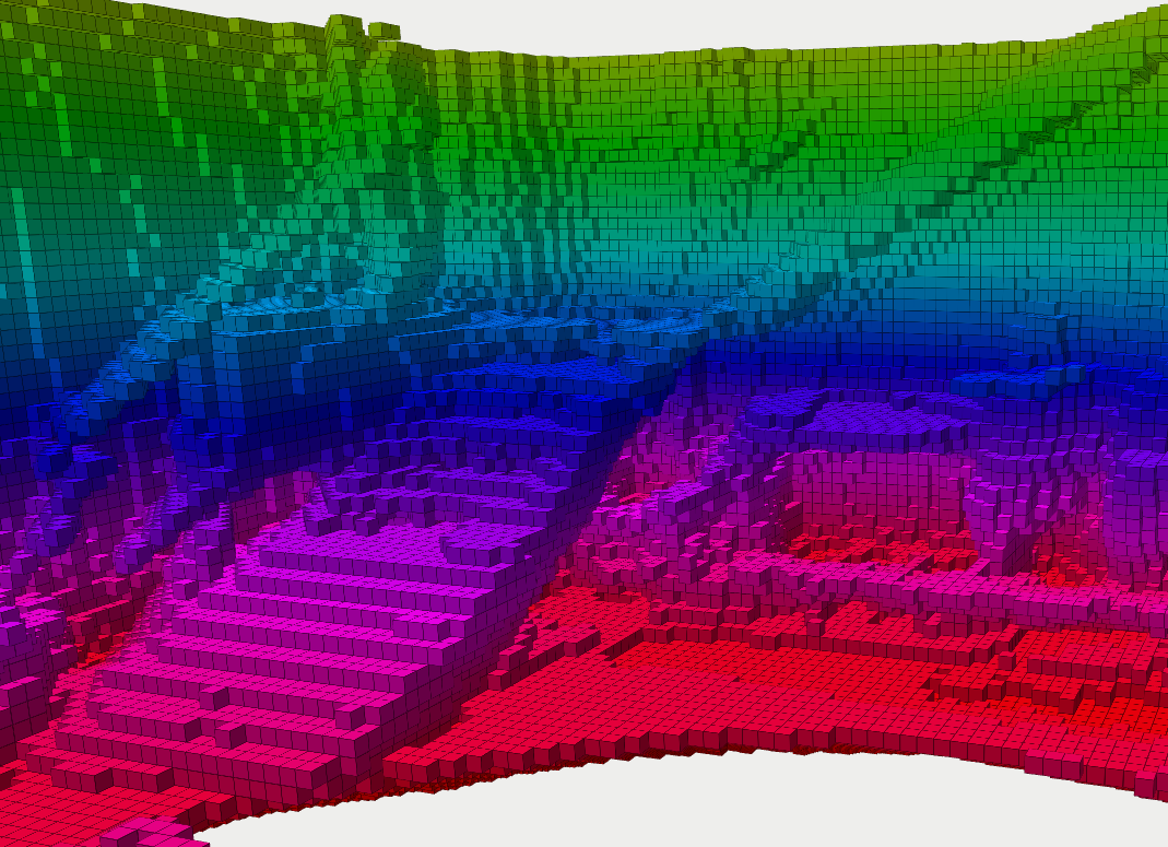
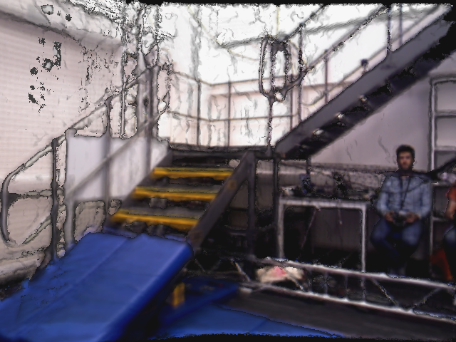
Figure 1: In this work, a light-weight exploration algorithm for MAVs was developed. [Left] The map created on-board the MAV in real-time using a voxel resolution of 10 cm which is used for exploration planning and collision avoidance. [Right] A high resolution render of a map created offline from the depth and colour images collected in the experiment. The map was created using the pipeline presented in [3].

II Related Work

A considerable amount of work is available on autonomous exploration. The utility metrics that drive the exploration can be grouped into two categories, map entropy metrics [4] and unknown volume metrics [5]. These metrics can be utilised by either of the two main exploration strategies which are sampling-based and frontier-based exploration.

In the original work on frontier exploration [6], the closest frontier from the current robot position is chosen. In [7], priority is given to maintaining a high MAV velocity during the exploration task. Gao et al. [8] focus on keeping track of visited key nodes in a topological graph while conducting frontier exploration. A more recent work on frontier-based autonomous inspection is presented in [9].

The core idea of the sampling-based exploration approach is to sample potential poses which could contribute to mapping the unknown volume. This strategy avoids the map-wide computation of frontiers but requires the evaluation of each sample. Bircher et al. [10] have shown that the Next-Best-View (NBV) method [11] can be applied in 3D exploration. The NBV is found by growing an RRT to sample a position and yaw angle in free space. This method is improved in [5] where a history of visited locations is maintained to avoid being stuck at local minima.

Exploration strategies using map entropy as the evaluation metric mostly use the Shannon entropy [12, 13, 14]. In [15], the combination of the Shannon and the Renyi entropy provides a utility function which balances between the robot localisation and map uncertainty. In [16], mapping is performed in 3D while motion planning is done in 2D to reduce computational complexity since an MAV typically flies at a constant height. Bissmarck et al. [17] compared various approaches to compute the information gain for candidate views. The proposed frontier oriented volumetric hierarchical ray tracing was benchmarked against the hierarchical ray-tracing by Vasquez-Gomez et al. [18] in computation time, mapping efficiency and estimation error.

The second group of evaluation metrics estimates the amount of unknown volume in the view frustum via ray casting. This metric is used in [5, 10, 19, 20, 21]. The latter two add secondary tasks which are achieved in parallel to the main exploration task.

III Problem Statement

Let $V\subset\mathbb{R}^{3}$ be a bounded volume whose points $\mathbf{v}\in V$ have the occupancy probabilities $P_{o}(\mathbf{v})$. The goal of autonomous exploration is to use a sensor-equipped robotic platform to create a map $M$ of all the observable space in $V$. In most non-trivial environments, there are points $V_{\mathrm{unob}}\subset V$ that can not be observed by the sensor, such as the interior of solid objects or passages too small for the robotic platform to explore. Thus the goal of autonomous exploration is to update the occupancy probability of all observable points by the sensors $V_{\mathrm{obs}}=V\setminus V_{\mathrm{unob}}$ to free or occupied. Another concept useful in exploration is that of frontiers. Frontiers are the boundaries between free and unknown space. They mark observable regions that can lead to an expansion of the map if observed. The exploration termination condition can be equivalently expressed in terms of frontiers as the state where there are no more frontiers left.

Initially, all points $\mathbf{v}\in V$ are unknown if no prior information is available and the robotic platform has to map and navigate the unknown space. Path planning, collision avoidance, and exploration planning have to be performed online as there is no a priori knowledge of the environment. Thus it is important for the whole exploration pipeline to run efficiently on-board the robotic platform.

In this paper we propose a solution to autonomous exploration using an MAV that is equipped with a depth sensor and is employing a volumetric map to represent the environment. The presented exploration strategy is iterative and is tightly coupled with the underlying map representation, as detailed in the following.

IV Frontier-based Information-driven Exploration Algorithm

We propose a frontier sampling, information gain-based exploration approach. It takes inspiration from both frontier-based and sampling-based exploration methodologies. Frontiers are good indicators of the regions the exploration should be focused on, which are ignored by conventional sampling-based exploration algorithms. By sampling candidate next-views at the frontiers there is no need for clustering of the individual voxels into larger frontiers, thus removing the associated large computational cost. A utility function expressing expected information gain over time is used to evaluate the candidate next-views. This is a more meaningful metric than just counting unobserved voxels and does not require a tuning parameter to take the path cost into account.

An occupancy mapping server [22] is kept running in the background, which continuously integrates depth image and pose pairs into the map and extracts the frontiers. At the beginning of the exploration and after some measurements have been integrated into the map, the exploration planner is called. At each planning iteration it executes the following steps in sequence:

1. A pre-defined number of candidate goal positions are sampled from frontier voxels (Section IV-D).

2. Collision-free paths from the current position to each candidate position are planned (Section IV-E).

3. A yaw angle is associated to each candidate position, creating a candidate pose, and each pose is evaluated based on a utility function expressing information gain over time (Section IV-F).

4. The candidate pose with the highest utility is selected as the next goal.

The map is continuously updated as the MAV moves towards the goal. Once the goal is reached, the next planning iteration begins. The exploration is considered complete when there are no more frontier clusters remaining. A graphical overview of the proposed approach is presented in Figure 2.

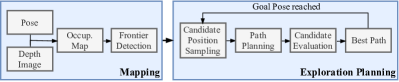
Figure 2: The mapping system runs continuously in the background while the exploration planner produces a new path each time the previous path is completed.

IV-A MAV Model

Our exploration method is specifically tailored for MAVs. It is assumed that the MAV’s state $\mathbf{x}$ consists of its position $\mathbf{p}=[x,y,z]^{T}\in V$ and yaw angle, $\psi\in[0,2\pi)$, relative to the World frame ${\smash{\underrightarrow{\mathcal{F}}_{W}}}$ thus $\mathbf{x}=[x,y,z,\psi]^{T}\in V\times[0,2\pi)$. It is also assumed that the MAV has a maximum linear velocity $\upsilon_{\max}\in\mathbb{R}^{+}$ and maximum yaw rate $\omega_{\max}\in\mathbb{R}^{+}$. The MAV is also equipped with a depth camera mounted on a fixed position, with maximum sensor range $d_{\max}\in\mathbb{R}^{+}$ and horizontal and vertical field of view $\alpha_{h}$ and $\alpha_{v}$ respectively. For collision checking, we assume the MAV is contained inside a sphere with centre $\mathbf{p}$ and safety radius $R\in\mathbb{R}^{+}$.

IV-B Map Representation

We chose to use an occupancy map for three main reasons. First, it provides an explicit representation of free space in which collision-free paths can be easily planned. Second, an occupancy map is also inherently suitable for integrating noisy sensor measurements. Finally, it provides an implicit measure of map quality through its entropy.

The occupancy mapping framework used in this work is supereight [22]. supereight uses an octree structure to store the map. An octree is a tree data structure each node of which subdivides the 3D space it corresponds to into 8 octants which are represented as its children nodes in the octree. supereight also provides efficient map updates and queries by using Morton codes for spatial indexing. Instead of storing single voxels at the octree leaf level, supereight stores blocks of voxels at the leaf level, typically $8\times 8\times 8$ voxels in size. The side length in meters of a single voxel is called map resolution and is denoted $r$. The map is continuously updated as new pose and depth image pairs arrive. The system does not assume any particular pose tracking method. Thus any system can be run in parallel to the exploration and provide an estimate of the MAV’s pose, e.g. a visual-inertial odometry pipeline or a motion capture system.

We extend supereight to store whether each voxel is a frontier and perform frontier detection, as described in the following section. Additionally, up-propagation of occupancy probabilities through the octree levels is performed to facilitate efficient collision queries: after a new depth measurement is integrated into the map, each parent node whose children were updated will also have its occupancy probability updated. Specifically, the occupancy probability of the parent is set to the maximum of the occupancy probabilities of its children. This way, if an octree node has an occupancy probability smaller than 0.5, it is guaranteed that its children also have an occupancy probability smaller than 0.5.

IV-C Frontier Detection

The map frontiers are detected during the map update process. The frontiers are stored as a sorted list $F$ containing Morton codes corresponding to voxel blocks (octree leaves) with one or more frontier voxels. An implicit frontier clustering at the voxel block level is achieved by considering voxels in the same voxel block as a frontier cluster. Thus any computationally intensive clustering methods as in [4] are avoided.

At each depth measurement integration into the map, the voxels inside the camera frustum are updated. Each of the updated voxels is tested for being a frontier voxel. Voxels are considered frontiers if their occupancy probability is lower than 0.5, while one or more of their 6 face neighbour voxels has an occupancy probability of exactly 0.5. More intuitively, frontier voxels are free voxels located next to completely unobserved voxels. The Morton code list is updated as new frontier voxels emerge and previously unobserved regions are observed. The latter leads to removal of frontier voxels. By only considering the last updated voxels for the map frontiers update, a map-wide operation is avoided. This frontier update is performed continuously at each sensor measurement integration.

IV-D Candidate Position Sampling

At the beginning of each planning iteration, a predefined number $N_{c}$ of candidate positions $\mathbf{p}_{i}=[x_{i},y_{i},z_{i}]^{T}\in\mathbb{R}^{3},\ i\in\{1\dots N_{c}\}$ is uniformly sampled from the frontier voxel blocks in $F$. Initially, the number of frontier voxels in each frontier voxel block is obtained. Frontier voxel blocks containing fewer frontier voxels given a certain threshold are ignored for the duration of the candidate position sampling, resulting in the filtered frontier list $\tilde{F}$. Since $\tilde{F}$ is sorted and due to the spatial indexing of Morton codes, a more spatially uniform candidate position sampling can be achieved by sampling every $\lceil N_{rem}/N_{c}\rceil$th frontier voxel block in $\tilde{F}$, where $N_{rem}$ is the number of frontier voxel blocks in $\tilde{F}$ and $\lceil\cdot\rceil$ denotes the ceiling of the argument. For each of the selected frontier voxel blocks, one of its frontier voxels is randomly selected and its coordinates used as a candidate position $\mathbf{p}_{i}$. The current MAV position is always added to the candidates to ensure that a rotation around the yaw axis without any movement is also considered as candidate pose.

IV-E Path Planning to Candidate Positions

The Open Motion Planning Library (OMPL) [23] is used for computing paths to the candidate positions. The integrated planning algorithm is the informed RRT* [24] with path simplification. The octree map structure is exploited to perform efficient collision checking. Free space queries are made by checking the occupancy probability against a threshold and are first performed at a higher octree level, before checking at the single-voxel level. A sphere around the MAV is used for collision checking for points and a cylinder for line segments. The path is computed in $\mathbb{R}^{3}$ and the corresponding yaw angles are computed at a later stage.

Since candidate positions are sampled at the frontier, hence close to unknown space, the MAV cannot safely reach them due to its finite dimensions. In this case, OMPL computes a collision-free path which ends before the candidate position, typically at a distance near the MAV’s safety radius. The candidate position is then updated to this safe path endpoint resulting in the path $W_{i}(\mathbf{p},\mathbf{p}_{i})$ from the current MAV position $\mathbf{p}$ to the updated candidate. The path consists of one or more line segments.

In receding horizon exploration methods [10, 25], the MAV moves only to the first point of a planned path before performing another planning iteration. This sometimes has the effect that the MAV moves back and forth in a small area since at subsequent planning iterations it may move to the first point of paths to different endpoints (i.e. from different frontiers). Thus the MAV is temporarily stuck in a small region. In our approach, the MAV follows the path to its endpoint, committing to exploring a single frontier before moving towards another goal.

IV-F Yaw Optimisation and Candidate Pose Evaluation

The map entropy is computed at each candidate position by performing a $360^{o}$ sparse raycasting. Each candidate position $\mathbf{p}_{i}$ is converted into a candidate pose $\mathbf{x}_{i}=[x_{i},y_{i},z_{i},\psi_{i}]^{T}$ by optimising the yaw angle for the highest entropy given the $360^{o}$ raycast. The estimated travel time to the candidate pose is computed based on the MAV’s maximum linear velocity $\upsilon_{\max}$ and maximum yaw rate $\omega_{\max}$. The utility function of a candidate goal pose is computed as the map entropy over the estimated path travel time. Finally the candidate pose with the highest utility is selected as the next goal pose. We will detail these steps in the following.

IV-F1 Sparse Raycasting and Yaw Optimisation

Instead of random sampling the MAV yaw angle using the informed RRT*, it is optimised by performing a sparse $360^{o}$ raycasting which at the same time computes the map entropy along each ray. It has been shown [26] that sparse raycasting can effectively approximate a full raycasting at a fraction of the computational cost.

Given the sensor’s vertical field of view $\alpha_{v}$ and its maximum range $d_{\max}$, the raycasting is performed with a horizontal angle increment $\delta\psi$ for the yaw angle and a vertical angle increment $\delta\theta$ for $\alpha_{v}$, with the rays being stopped at a distance $d_{\max}$ from $\mathbf{p}_{i}$. The entropy for a single voxel $\mathbf{v}$ is calculated using Shannon’s information theory

$$\mathbb{H}(\mathbf{v})=-P_{o}(\mathbf{v})\ln P_{o}(\mathbf{v})-\left(1-P_{o}(\mathbf{v})\right)\ln\left(1-P_{o}(\mathbf{v})\right),$$ (1)

where $\mathbb{H}(\mathbf{v})$ denotes the map entropy and $P_{o}(\mathbf{v})$ the occupancy probability of a voxel $\mathbf{v}$.

The entropy along a ray is computed as the sum of the entropy of the voxels along the ray until the first voxel $\mathbf{v}$ with $P_{o}(\mathbf{v})>0.5$ or $d_{\max}$ is reached, whichever comes first. By taking into account the entropy of both observed and unobserved voxels, we evaluate both unknown regions and regions where the map is still uncertain and of low quality. Thus it acts as a measure of both map coverage and quality. The raycasting is performed on the current map and computes a $360^{o}$ estimated entropy map, with each pixel corresponding to a single ray, like the one shown in Figure 3 [Bottom]. The brighter a pixel is, the higher the entropy for the corresponding ray. The corresponding sparse depth map is shown in Figure 3 [Top]. Lighter shades of grey denote rays that hit an occupied voxel closer to the candidate position, while black denotes rays that did not hit any occupied voxels up to a distance $d_{\max}$, producing an invalid depth measurement. This can be either due to free space extending to a distance greater than $d_{\max}$ or due to the existence of voxels with high map entropy, as is the case for the rightmost and leftmost invalid depth regions respectively in Figure 3 [Top].

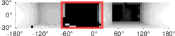
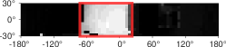
Figure 3: Sparse raycasted depth map [Top] and corresponding entropy map [Bottom]. The boundaries of the camera frustum at the yaw angle that results in the highest map entropy are shown in red.

In order to obtain the optimal yaw for the candidate position, a sliding window summation with an angular width $\alpha_{h}$ is performed on the entropy map. For each yaw value, the sum of the entropy of the rays that fall inside the sensor’s field of view is computed. The yaw angle $\psi_{i}$ with the highest cumulative map entropy is selected, resulting in the candidate pose $\mathbf{x}_{i}$. We use $\mathbb{H}(\mathbf{x}_{i})$ to denote the map entropy obtained by raycasting from candidate pose $\mathbf{x}_{i}$. The boundaries of the camera frustum at the yaw angle that results in the highest map entropy are shown in red in Figure 3.

IV-F2 Utility Function

The utility for a candidate pose $\mathbf{x}_{i}$ given the path $W_{i}$ to it is the entropy of the portion of the map visible from the pose over the time it takes to complete the path $W_{i}$. This results in a balance between exploring the MAV’s immediate surroundings by penalizing time-consuming paths and moving towards more distant frontiers leading to potentially completely unexplored regions by favouring high map entropy. By formulating the utility as a ratio, this balance is achieved without the need for any tuning parameter.

The estimated information gain computation using sparse raycasting was described in the previous section. The estimated time $T(W_{i})$ to complete path $W_{i}$ is computed by assuming the MAV always flies at its maximum linear speed and rotates at the maximum rate when needed. Thus the total path travel time $T(W_{i})$ is estimated as the maximum between the time the MAV needs to move from its start point $\mathbf{p}$ to its final point $\mathbf{p}_{i}$ at $\upsilon_{\max}$ and the time it takes to rotate from the start yaw $\psi$ to its final yaw $\psi_{i}$ at $\omega_{\max}$. Although this estimate is not accurate due to the constraints imposed by the MAV’s dynamics, it is a suitable approximation. The utility function serves to provide a ranking of the candidate poses.

Thus the utility of a candidate pose is computed as

$$u(\mathbf{x}_{i},\hat{W_{i}})=\frac{\mathbb{H}(\mathbf{x}_{i})}{T(\hat{W_{i}})},$$ (2)

and the candidate pose $\hat{\mathbf{x}}_{i}=[\hat{\mathbf{p}}_{i}^{T}\hat{\psi}_{i}]^{T}$ with the highest utility is selected as the next goal pose.

Since the path $W_{i}(\mathbf{p},\hat{\mathbf{p}}_{i})$ consists of a number of points with no associated yaw, each point in the path has to be matched to a yaw angle before it is supplied to the MAV’s controller. The initial and final points of the path already have associated yaw angles $\psi$ and $\hat{\psi}_{i}$ from the current $\mathbf{x}$ and best candidate pose $\hat{\mathbf{x}}_{i}$ respectively. For each intermediate path point a yaw angle is assigned by performing the same yaw optimisation as for $W_{i}(\mathbf{p},\mathbf{p}_{i})$, resulting in the final path $\hat{W_{i}}(\mathbf{x},\hat{\mathbf{x}}_{i})$ to the goal pose. Essentially, for each intermediate point of the path to the best candidate pose a sparse raycasting and related map entropy computation is performed. The number of intermediate points depends on the geometry of the space but due to the OMPL path simplification it is in general low. Since this intermediate yaw optimisation is performed only for the path to the best candidate, its effect on the total computation time is limited.

V Experimental Evaluation

The exploration algorithm has been evaluated in both simulated and real world experiments. All simulated experiments were performed in Ubuntu 18.04 using ROS Melodic and the RotorS simulator [27]. The MAV model used in the simulation is the Ascending Technologies FireFly hexacopter equipped with a VI-Sensor mounted at a $15^{\circ}$ angle. For all simulations 20 candidate poses are sampled at each planner iteration. All simulations were run on an Intel Core i7-8750H CPU operating at 2.20 GHz and compiled with g++ 7.4.0 using the O3 optimization level. The parameters used for both the simulated and real-world experiments can be found in Table I.

V-A Apartment Environment Simulation

Several simulations were conducted in the 10 m $\times$ 20 m $\times$ 3 m apartment environment used in [10, 25]. Our algorithm was compared with the NBV planner presented in [10]. Figure 4 shows the explored volume over time, averaged over 10 runs, for both algorithms using a voxel resolution of $r=0.1$ m and $r=0.4$ m. It can be observed that our method explores the whole environment substantially faster, especially when using a high resolution map. An interesting property of our method is that it does not require any arbitrary initialisation movement, like the $360^{\circ}$ in-place rotation in [10]. Instead, the utility function usually gives higher utility to candidate poses that result in the MAV performing a similar rotation in the beginning of the exploration. Our method explores $95\%$ of the environment in 80 s and 151 s for a resolution of 0.4 m and 0.1 m respectively. These are lower than the respective times reported in [25], although it should be noted that we were unable to run their planner on our hardware, despite our best efforts, so the results might not be directly comparable, especially since the hardware used by the authors is not stated.

TABLE I: Exploration parameters

Parameter	Apartment	Maze	Powerplant	Experiment
$r$ (m)	0.1, 0.4	0.1, 0.2	0.2	0.1
$R$ (m)	0.5	0.5	0.5	0.8
$\upsilon_{\max}$ (m/s)	1.5	1.5	0.7, 1.5, 2.5	0.1
$\omega_{\max}$ (rad/s)	0.75	0.75	0.75	0.15
$d_{\max}$ (m)	5	5	7	4
$[\alpha_{h},\alpha_{v}]$	$[90^{\circ},60^{\circ}]$	$[115^{\circ},60^{\circ}]$	$[115^{\circ},60^{\circ}]$	$[58^{\circ},45^{\circ}]$

Figure 4: Apartment environment explored volume over time.

V-B Maze Environment Simulation

Simulations were also conducted in a more complex 20 m $\times$ 20 m $\times$ 2.5 m maze environment from [28]. Figure 5 shows the explored volume over time, averaged over 10 runs, for both our algorithm and NBVP using a voxel resolution of 0.1 m and 0.2 m. The planners were not run at a resolution of 0.4 m because this environment contains some narrow corridors that the MAV cannot navigate through when such a coarse resolution is used. Our method performs significantly faster than NBVP in this case since the random sampling of NBVP does not always detect unexplored regions quickly. This results in the MAV being stuck in a portion of the map for a long time before moving towards unexplored regions. Our planner does not exhibit this behaviour due to its use of frontiers which reliably guide the MAV towards unexplored space. Our method explores $95\%$ of the environment in 177 s and 330 s for a resolution of 0.2 m and 0.1 m respectively. Figure 6 shows a top-down view of a map created by our algorithm in the maze environment.

Figure 5: Maze environment explored volume over time.

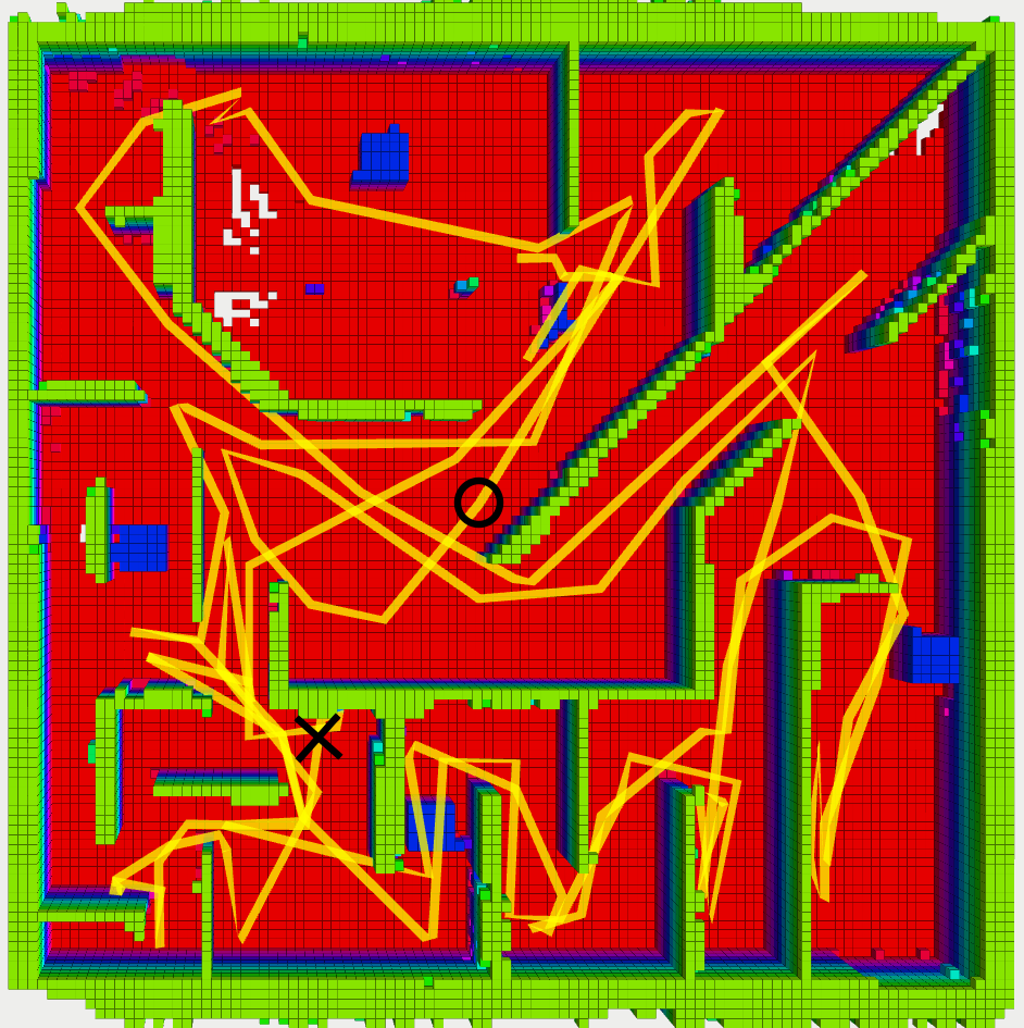
Figure 6: Top-down view of a map of the maze environment created by our algorithm. Voxels are coloured based on their height, with red indicating floor voxels and green voxels near the cropped roof. The MAV’s starting position is marked by a black circle, it’s path by a yellow line and it’s final position by a black cross.

V-C Powerplant Environment Simulation

In order to evaluate our method in an outdoors scenario, the 33 m $\times$ 31 m $\times$ 26 m powerplant environment from the Gazebo simulator was used. Figure 7 [Right] shows the explored volume over time, averaged over 10 runs, for various MAV maximum linear velocities. Figure 7 [Left] shows a map created by our algorithm and the corresponding MAV path. In this simulation, the planner is unable to explore the whole space because a large portion of it is unobservable, e.g. the interior of the building. For lower MAV velocities the exploration is slower not only due to the lower movement speed but because candidate views further away have a lower information gain over time due to the increased time it takes to fly to then. Thus the MAV more thoroughly explores the nearby regions before moving to ones further away. The same environment has been used to evaluate [29] and [25] by reporting only the time required to complete the exploration. However, since both [29] and [25] use different exploration termination conditions, a comparison of the completion time would not necessarily be indicative of a planner’s performance. A more meaningful comparison could be made by comparing the amount of volume explored in a given amount of time, as presented in Figure 7 [Right].

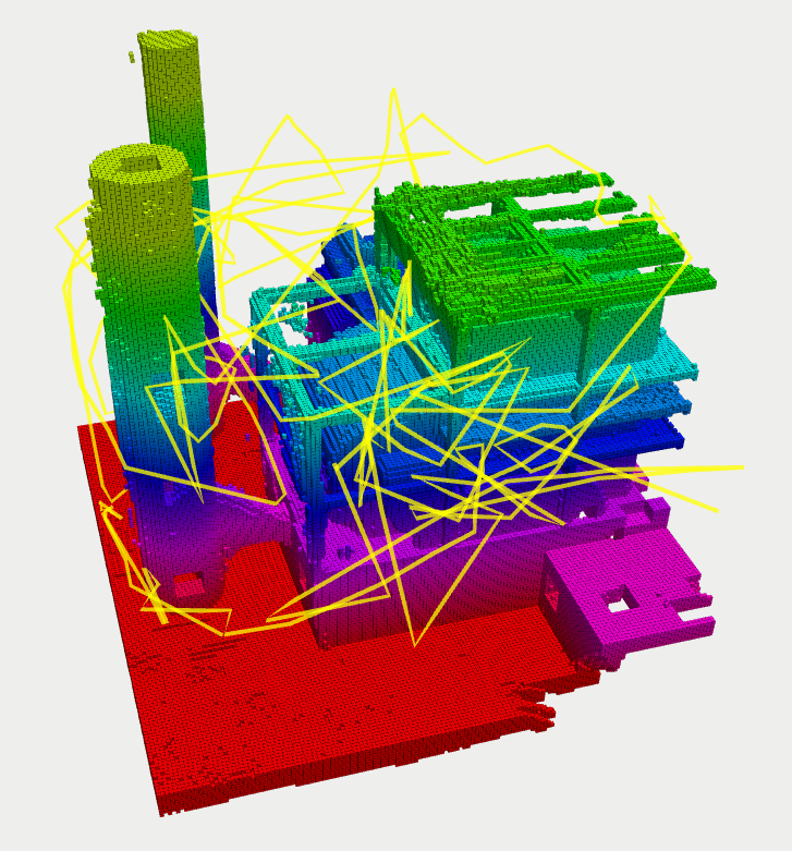
Figure 7: [Left] A map of the powerplant environment created by our method. Voxels are coloured based on their height and the MAV’s path through the environment is marked by a yellow line. [Right] Powerplant environment explored volume over time.

V-D Computational Complexity

Since the planner is running on-board an MAV its computational complexity is an important characteristic. Sampling the candidate positions has a complexity of $\text{O}(N_{c})$ and computing a single collision free path with $N_{p}$ points is $\text{O}(\frac{N_{p}-1}{r^{3}})$. Performing a single sparse raycast with $n$ horizontal rays and $m$ vertical rays scales with $\text{O}(\frac{nm}{r})$ while the yaw optimization scales with $\text{O}(n)$. Computing the utility of a single path requires computing its length, thus it scales with $\text{O}(N_{p})$. Finally, for the best path only, the yaw at the intermediate path points is computed with a sparse raycast and yaw optimization for each point giving $\text{O}(N_{p}(\frac{nm}{r}+n))$. Putting it all together, the computational complexity for a single planner iteration is $\text{O}\left(N_{c}\left(\frac{N_{p}}{r^{3}}+\frac{nm}{r}+n+N_{p}\right)+N_{p}\left(\frac{nm}{r}+n\right)\right)$.

For a quantitative comparison to other methods the per-iteration planner computation time for all simulations was measured. The mean and standard deviation for the three simulated environments at different map resolutions for both our planner and NBVP are presented in Table II. The reduction in computational time at higher resolutions can be attributed to the sparse raycasting, the efficient collision checking performed by our method. It should be noted that receding horizon planners like [10] and [25] typically perform a large number of planning iterations since they perform only a portion of the computed path at each iteration. Our algorithm performs relatively few planning iterations since each computed path is followed until its end before replanning.

TABLE II: Per-iteration computation time

	$r$ (m)	Apartment (ms)		Maze (ms)		Powerplant (ms)
Ours	0.4	122	$\pm$ 36		–		–
	0.2	156	$\pm$ 109	155	$\pm$ 71	152	$\pm$ 20
	0.1	68	$\pm$ 27	238	$\pm$ 80		–
NBVP	0.4	73	$\pm$ 8		–		–
	0.2	707	$\pm$ 44	775	$\pm$ 50		–
	0.1	7940	$\pm$ 410	8540	$\pm$ 425		–

V-E Real World Experiments

A real world experiment was performed in order to demonstrate the feasibility of running the proposed exploration algorithm on-board an MAV. The experiment was conducted in a 7 m $\times$ 5.5 m $\times$ 5 m room equipped with a VICON motion capture system providing the MAV pose. The MAV used was a DJI F550 hexacopter equipped with an ASUS Xtion Pro RGBD camera. The entire system, both mapping and exploration planning was run on-board the MAV on an Intel NUC with an Intel Core i7-7567U CPU operating at 3.5 GHz. After a manual take-off to a height of 1 m by the safety pilot, the exploration algorithm is initiated. A 0.5 m $\times$ 1.3 m $\times$ 0.8 m obstacle was placed inside the room in order to create additional frontiers and force the MAV to navigate around it. The mean per-iteration computation time was 383 ms with a standard deviation of 144 ms. The resulting map can be seen in Figure 8 [Left] and a photograph of the experimental setup in Figure 8 [Right].

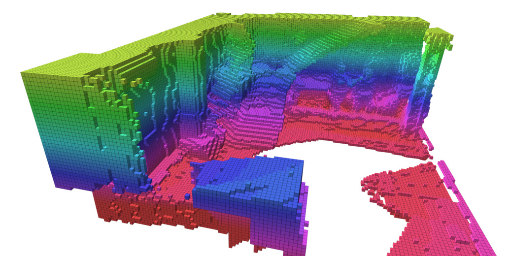
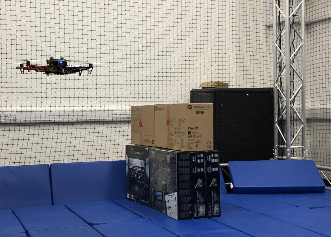
Figure 8: [Left] Map of the room the experiment was conducted in. Voxels are coloured based on their height and two of the walls have been cropped for visualization. [Right] A photograph of the MAV and the obstacle.

VI Conclusions and Future Work

In this work, we have presented an exploration strategy that is a hybrid between frontier-based and sampling-based strategies. It improves upon the state-of-the-art both in terms of exploration speed and computational cost as shown in the simulation studies. The real-world experiment showcases that it is feasible to use the proposed strategy in the real world and that it can be run in real-time on-board an MAV.

In future work we are planning on using a multi-resolution mapping pipeline like the one in [3] and generating dynamically feasible drone trajectories instead of a series of waypoints. More planned improvements include the use of additional sensor types such as LIDARs, robust operation in real-world outdoor environments and the ability to explore and navigate dynamic environments.

References

- [1] M. Juliá, A. Gil, and Ó. Reinoso, “A comparison of path planning strategies for autonomous exploration and mapping of unknown environments,” Autonomous Robots, vol. 33, pp. 427–444, 2012.
- [2] S. M. LaValle, Planning Algorithms. Cambridge University Press, 2006.
- [3] E. Vespa, N. Funk, P. H. Kelly, and S. Leutenegger, “Adaptive-resolution octree-based volumetric SLAM,” in 2019 International Conference on 3D Vision (3DV). IEEE, Sep 2019, pp. 654–662.
- [4] B. Charrow, S. Liu, V. Kumar, and N. Michael, “Information-theoretic mapping using Cauchy-Schwarz quadratic mutual information,” in 2015 IEEE International Conference on Robotics and Automation (ICRA), May 2015, pp. 4791–4798.
- [5] C. Witting, M. Fehr, R. Bähnemann, H. Oleynikova, and R. Siegwart, “History-aware autonomous exploration in confined environments using MAVs,” in 2018 IEEE/RSJ International Conference on Intelligent Robots and Systems (IROS), Oct 2018, pp. 1–9.
- [6] B. Yamauchi, “A frontier-based approach for autonomous exploration,” in Proceedings of IEEE International Symposium on Computational Intelligence in Robotics and Automation, CIRA, Oct 1997, pp. 146–151.
- [7] T. Cieslewski, E. Kaufmann, and D. Scaramuzza, “Rapid exploration with multi-rotors: A frontier selection method for high speed flight,” in 2017 IEEE/RSJ International Conference on Intelligent Robots and Systems (IROS), Sep 2017, pp. 2135–2142.
- [8] W. Gao, M. Booker, A. H. Adiwahono, M. Yuan, J. Wang, and W.-Y. Yau, “An improved frontier-based approach for autonomous exploration,” 2018 15th International Conference on Control, Automation, Robotics and Vision (ICARCV), pp. 292–297, 2018.
- [9] M. Faria, I. Maza, and A. Viguria, “Applying frontier cells based exploration and lazy theta* path planning over single grid-based world representation for autonomous inspection of large 3D structures with an UAS,” Journal of Intelligent & Robotic Systems, vol. 93, no. 1, pp. 113–133, Feb 2019.
- [10] A. Bircher, M. Kamel, K. Alexis, H. Oleynikova, and R. Siegwart, “Receding horizon path planning for 3D exploration and surface inspection,” Autonomous Robots, vol. 42, no. 2, pp. 291–306, Feb. 2018.
- [11] C. I. Connolly, “The determination of next best views,” Proceedings. 1985 IEEE International Conference on Robotics and Automation, vol. 2, pp. 432–435, 1985.
- [12] E. Palazzolo and C. Stachniss, “Information-driven autonomous exploration for a vision-based MAV,” ISPRS Annals of Photogrammetry, Remote Sensing and Spatial Information Sciences, vol. IV-2/W3, pp. 59–66, 08 2017.
- [13] M. Scott and K. Jerath, “Multi-robot exploration and coverage: Entropy-based adaptive maps with adjacency control laws,” 2018 Annual American Control Conference (ACC), pp. 4403–4408, 2018.
- [14] E. Palazzolo and C. Stachniss, “Effective exploration for MAVs based on the expected information gain,” Drones, vol. 2, no. 1, 2018.
- [15] H. Carrillo, P. Dames, V. Kumar, and J. Castellanos, “Autonomous robotic exploration using a utility function based on Renyi’s general theory of entropy,” Autonomous Robots, vol. 42, 08 2017.
- [16] E. Kaufman, K. Takami, Z. Ai, and T. Lee, “Autonomous quadrotor 3D mapping and exploration using exact occupancy probabilities,” in 2018 Second IEEE International Conference on Robotic Computing (IRC), Jan 2018, pp. 49–55.
- [17] F. Bissmarck, M. Svensson, and G. Tolt, “Efficient algorithms for next best view evaluation,” in 2015 IEEE/RSJ International Conference on Intelligent Robots and Systems (IROS), Sep 2015, pp. 5876–5883.
- [18] J. I. Vasquez-Gomez, L. E. Sucar, and R. Murrieta-Cid, “Hierarchical ray tracing for fast volumetric next-best-view planning,” 2013 International Conference on Computer and Robot Vision, pp. 181–187, 2013.
- [19] J. Delmerico, S. Isler, R. Sabzevari, and D. Scaramuzza, “A comparison of volumetric information gain metrics for active 3D object reconstruction,” Autonomous Robots, vol. 42, no. 2, pp. 197–208, 2018.
- [20] T. Dang, C. Papachristos, and K. Alexis, “Visual saliency-aware receding horizon autonomous exploration with application to aerial robotics,” 2018 IEEE International Conference on Robotics and Automation (ICRA), pp. 2526–2533, 2018.
- [21] C. Papachristos, S. Khattak, and K. Alexis, “Uncertainty-aware receding horizon exploration and mapping using aerial robots,” in 2017 IEEE international conference on robotics and automation (ICRA), 05 2017, pp. 4568–4575.
- [22] E. Vespa, N. Nikolov, M. Grimm, L. Nardi, P. H. J. Kelly, and S. Leutenegger, “Efficient octree-based volumetric SLAM supporting signed-distance and occupancy mapping,” IEEE Robotics and Automation Letters, vol. 3, no. 2, pp. 1144–1151, Apr. 2018.
- [23] I. A. Sucan, M. Moll, and L. E. Kavraki, “The open motion planning library,” IEEE Robotics Automation Magazine, vol. 19, no. 4, pp. 72–82, Dec 2012.
- [24] J. D. Gammell, S. S. Srinivasa, and T. D. Barfoot, “Informed RRT*: Optimal sampling-based path planning focused via direct sampling of an admissible ellipsoidal heuristic,” 2014 IEEE/RSJ International Conference on Intelligent Robots and Systems, pp. 2997–3004, 2014.
- [25] M. Selin, M. Tiger, D. Duberg, F. Heintz, and P. Jensfelt, “Efficient autonomous exploration planning of large-scale 3-D environments,” IEEE Robotics and Automation Letters, vol. 4, no. 2, pp. 1699–1706, 2019.
- [26] H. Oleynikova, Z. Taylor, R. Siegwart, and J. Nieto, “Safe local exploration for replanning in cluttered unknown environments for microaerial vehicles,” IEEE Robotics and Automation Letters, vol. 3, no. 3, pp. 1474–1481, 2018.
- [27] F. Furrer, M. Burri, M. Achtelik, and R. Siegwart, Robot Operating System (ROS): The Complete Reference (Volume 1). Cham: Springer International Publishing, 2016, ch. RotorS—A Modular Gazebo MAV Simulator Framework, pp. 595–625.
- [28] H. Oleynikova, Z. Taylor, M. Fehr, R. Siegwart, and J. Nieto, “Voxblox: Incremental 3D Euclidean signed distance fields for on-board MAV planning,” in IEEE/RSJ International Conference on Intelligent Robots and Systems (IROS), 2017, https://github.com/ethz-asl/mav_voxblox_planning, accessed Aug. 2019.
- [29] T. Cieslewski, E. Kaufmann, and D. Scaramuzza, “Rapid exploration with multi-rotors: A frontier selection method for high speed flight,” in 2017 IEEE/RSJ International Conference on Intelligent Robots and Systems (IROS). IEEE, 2017, pp. 2135–2142.